
Submitted:
12 March 2025
Posted:
12 March 2025
You are already at the latest version
Abstract
In the current energy landscape, efficiency is a critical topic. Therefore, even in the case of geared transmissions, it is essential to predict and calculate power losses as accurately as possible from the design phase. There are mainly three categories of losses in a gear unit: friction - the power losses due to the contact between teeth in rotation on the one hand and the seals with the spindles on the other hand, churning - the power losses generated by the air-lubricant mixture compression around teeth roots during rotation and windage - the power losses due to the teeth aerodynamic trail in the air-lubricant mixture. While the first two categories of losses are intensively studied in the literature, the papers focusing on windage power losses are less representative. Estimation of windage power losses can be done by numerical simulation, the accuracy of the results depending on the mesh density and the available computing power. The present study discusses the influence of meshing on the windage torque of an orthogonal face gear immersed in air and compares numerical results generated by SolidWorks Flow Simulation software with experimental data measured on a test rig.
Keywords:
convergence
; face gear
; flow simulation
; torque
; windage
1. Introduction
The Windage power losses (WPL) in gears, particularly in high-speed applications, are a significant concern due to their impact on transmission efficiency. These losses arise from the interaction between the rotating gear surfaces and the surrounding air or lubricant, leading to energy dissipation [1,2,3,4]. Various studies have explored methods to quantify and mitigate these losses. For instance, Ruzek et al. [5] revealed that optimal modification of tooth geometry is able decrease WPL, but there is an optimal modification beyond which losses increase.
Li and Wang [6] further developed a calculation method for windage power losses in spiral bevel gears, emphasizing the influence of gear speed and geometry on these losses, and highlighting the role of lubricating oil in increasing windage losses. Their subsequent study [7] using oil injection lubrication confirmed the significant impact of lubrication parameters on windage power losses, providing a comprehensive analysis of the fluid dynamics involved.
In an earlier research, Ruzek et al. [8] presented an original test device which allows the measurement of wind losses for a pinion-gear pair, as opposed to classical devices limited to a single rotating element. Their study confirmed that the WPL result is close to the result obtained by summing the losses for each element considered individually. However, it appears that the air flow generated by one element may act on the other element to some extent, thus leading to overall WPLs slightly lower than those obtained by adding individual losses. The amount of power loss due to wind at the highest wind speeds can reach several kW, indicating that windage is essential in some applications.
In the study [9], Al-Shibl et al. explored non-dimensional shroud spacings between 0.005 and 0.05 at shaft speeds ranging from 5000 rpm to 20000 rpm. While it was observed that the Computational Fluid Dynamics (CFD) data closely matched the experimental results, an optimum tolerance could not be identified. Additionally, it was found that modifying the tooth tip by adding a small chamfer on the leading edge reduced the WPL by about 6%. A small bevel increased total WPL by a similar amount, suggesting that the WPL may rise as the gear wears down.
Recently, Dai et al. [10] investigated the windage and churning behaviors in different gear types, finding that spatial intersecting cross-axis gears like bevel and face gears exhibit higher no-load power losses compared to parallel-axes gears.
The use of shrouds has been proposed as a strategy to reduce windage losses by enclosing the gears, as demonstrated by Dai et al. They involved the Lattice Boltzmann method to simulate and validate the reduction in windage power losses in shrouded spur gears [11]. Furthermore, they introduced a torque containment factor that accounts for air compressibility at high Mach numbers, leading to improved theoretical formulae for predicting windage power losses, which enhances the applicability of these predictions during the preliminary design stage of shrouded gears.
Handschuh et al. [12] revealed through experimental results that even a loose shroud on the gears, operating at a remarkable pitch line velocity, can significantly minimize windage power losses, showcasing the power of innovation and resilience in engineering.
Marchesse et al. [13] conducted experiments to better understand how single-side and double-side baffles affect the drag losses of helical and spur gears. Their findings revealed something important: for spur gears, using symmetrical flanges consistently helps to lower windage losses, no matter the size of the clearance. It’s fascinating to see how even a single axial flange can make a difference in reducing these losses. On the other hand, when it comes to helical gears, they found that a flange positioned close to the discharge side doesn’t have as significant an impact on reducing windage losses as one placed on the intake side.
As can be observed, these studies collectively offer valuable insights into the mechanisms of windage power losses and potential strategies for their reduction, crucial for enhancing the efficiency of gear transmissions in high-speed applications. While the rotational speed of gears, the geometrical characteristics of gear design, and the density of the surrounding fluid are undeniably significant factors, the specific impact of these elements on power loss is not yet fully elucidated. Furthermore, although various solutions have been proposed to reduce power loss, their overall effectiveness in diverse operational scenarios remains uncertain and requires further scholarly examination. In addition, recent research increasingly relies on the results obtained from numerical simulations using CFD software tools. It is well known that the accuracy of these results largely depends on the refinement of the model and the available computing power.
Starting from this fact, in this study we aimed to assess the influence of the used mesh density, respective the cell numbers, on the simulation results. For this purpose, we created a virtual model identical to the one used by Zhu and Dai [14], who experimentally measured the windage torque of a 3D-printed orthogonal face gear made of 9400 resin, which was placed inside a parallelepiped gearbox housing made of Plexiglas, without oil. The results of the simulation were close to the experimental ones, the higher the refinement grade, obtaining almost identical results in the case of using a number of 689605 cells for meshing the face gear.
The following sections of this paper are organized as follows: Section 2 presents the theoretical foundations of the study, including computational methods for a generalized analytical model used to evaluate windage drag torque. Section 3 details the materials and methods used in the study, while Section 4 presents the results obtained and Conclusions are presented in Section 5.
2. Theoretical Background
According to [15], at gear transmissions, because of the coexistence of windage and churning behaviors inside the housing, the windage drag torque Twind can be obtained as a product of the windage contributions factor λ and the gear windage torque without the oil Twind0:
Twind = λTwind0,
The windage contributions factor is crucial for estimating both windage power losses and total power losses. Since windage losses are proportional to the total surface area exposed to the airflow, this factor is calculated by taking the ratio of the air-wetted surface area to the total area of the gear:
where:
Sw- air-wetted surface of the gear;
S- total area of the gear;
Øw- oil immersion angle of the gear;
h- oil immersion depth of the gear;
Rp- the pitch radius of the gear.
Expressing the pitch radius of the gear as:
where:
z- number of teeth;
mn- normal module;
β- gear helix angle,
Equation (1) becomes:
Furthermore, the oil-wetted surface area, which includes the contact between the gear and the lubricating oil, can generally be expressed as the lateral surfaces of the front/rear faces and the tooth surfaces [16]:
where:
b- gear width;
αp- pressure angle at pitch point.
The windage drag torque and the related energy losses occurring without oil can be clearly divided into two components: the torque exerted on the flanks (Tflank) and the torque exerted on the teeth (Tteeth):
Twind0 = 2Tflank + Tteeth
Depending on the flow regime, based on boundary layer theory, Seetharaman et al. [17,18] proposed following relations for the windage drag torque exerted on the flanks Tflank:
a) for the laminar regime (Re < 105):
where:
- air density;
υair- kinematic viscosity of air;
V- tangential velocity at the pitch point.
b) for the turbulent regime (Re > 106):
For both upper mentioned cases, the Reynolds number is computed as:
where is the air viscosity.
Based on the concept of the active surface of teeth proposed by Diab et al. [19], the formula for the drag torque acting on the teeth surface, Tteeth, is expressed as:
in which:
where:
ξ- reduction factor caused by the inhibiting effect of the gearbox casing on the windage losses generated in the teeth space;
xa- tooth profile shift coefficient;
αA- pressure angle at tooth tip.
The windage torque is finally obtained as:
a) for laminar regime:
or:
b) for turbulent regime:
or:
3. Materials and Methods
3.1. Test Stand and Experimental Results
As previously mentioned, Zhu and Dai [14] published experimental data measured on a 3D printed face gear made of 9400 resin. Their test bench (Figure 1) included:
- a high-speed electric motor (HSEM) to drive a shaft which supports a face gear (FG);
- 2 bearings (B1 and B2);
- a dynamic torque transducer (DTT) with an accuracy of 0.001 Nm;
- a transparent parallelepiped housing (H) (394x 266x 100 [mm]) made of Plexiglas.
The geometrical parameters of the face gear are presented in Table 1.
The tests were performed at rotating speeds of 1000, 2000 and 3000 rpm, the evolution of the measured windage torque being illustrated in Figure 2.
3.2.3. D Model of the Gearbox
Staring from the above-mentioned information regarding the test stand, provided in [14], the generation of the gear 3D geometry was initiated by using KISSsoft software [20]. The model was exported as stp- file and was integrated in the assembly generated in SolidWorks software. The gear geometry and the 3D model of the gearbox assembly are shown in Figure 3.
3.3. Flow simulation settings
To perform the simulation in the Flow Simulation module of SolidWorks, the following steps have been performed:
1. Creation of Flow Simulation project
2. Definition of analysis type and control volume
3. Specifying the boundary conditions
4. Specification of convergence criteria;
5. Calculation of flow studies/ projects;
6. Visualization of the results.
Table 2, respectively Figure 4 are presenting the general settings of the simulation project. Furthermore, the Rotating Region was set to specify a local rotating frame of reference and analyze fluid flow through rotating components of the model.
In this simulation, for defining the Rotating Region, was created a disc with a diameter of 166 mm and a width of 17 mm, which included the gear geometry. Additionally, the angular velocity of this component had to be specified (Figure 5).
The SolidWorks Flow Simulation module analyses the assembly geometry and automatically generates the computational domain that includes the analyzed geometry. Figure 6 depicts the three-dimensional computational domain, which encompasses the assembly through a parallelepiped. The computational domain represents the region where flow calculations are conducted, and domain boundaries are parallel to the global coordinate system planes.
Meshing affects both the computation time and the accuracy of the results. To assess the refinement grade on the solution convergence, four mesh densities were imposed, according to Table 3. Figure 7 illustrates for comparison the four types of gear discreditation.
The four projects were performed on two computers with the configurations shown in Table 4.
4. Results and Discussion
In parallel with the running of the four simulations, starting from the variation form illustrated in Figure 2, the curve was digitized, using the PyDigitizer module [21]. Digitizer is a module for digitizing 2D curves from images, created with the help of free and Open-Source resources, using Python as a programming language. The installation kit is available as a dataset at Mendeley [22] for free installation and use of it. The operating procedure is explained in a video tutorial available on YouTube channel [23]. The result of the digitization is shown in Figure 8, together with the variation equation.
Performing the simulation for the four defined mesh densities the results which were obtained are shown in Table 5. The table presents, besides the computed windage torque (WT) values at the three rotating speeds (1000, 2000 and 3000 rot/min), the number of iterations, the central processing unit (CPU) time and the hard disk drive (HDD) size of each study.
To get a better understanding of the differences between the experimental results and the simulation results, Table 6 provides the percentage differences (Diff.) between these values. As [14] doesn’t provide concrete data on WT, but only their variation curve (Figure 2), as a function of speed, the comparison was made with the values resulting from the digitization of this curve.
The analysis reveals that the percentage differences between the experimental results and the simulations exhibit a notable decrease as the number of mesh cells increases. Specifically, the average percentage difference is observed to be 73.5% at simulations performed with 35964 mesh cells, indicating a substantial deviation between the experimental and simulated data. A significant deviation is also observed in the case of the usability of 100530 cells. In contrast, this discrepancy diminishes significantly to 18.4% by making the simulation with 316775 cells and to 10% when the number of mesh cells is increased to 689605. For a clearer picture of the influence of mesh refinement on the simulation results, Figure 9 shows the variation of WT results as a function of speed and number of cells. This trend emphasizes the critical role of mesh refinement in enhancing the accuracy of simulation outcomes
The above conclusion is further reinforced by the convergence chart shown in Figure 10. It is evident that as the number of cells increases, the windage torque values obtained from the simulation become increasingly similar to the experimentally measured values, and the convergence curve begins to flatten.
This finding is also confirmed by several research [24,25,26], which also reveal that fineness of discretization in numerical simulations significantly affects the accuracy of the results, as it determines the granularity of the computational model. Finer discretization generally leads to more accurate results but involves increased computational resources and time. In this sense, Figure 11 provides an image of the variation of computational resources (average CPU time and HDD size) consumed by the numerical simulation, depending on the number of cells.
As one can observe, discretization impacts both the computational efficiency and the precision of the outcomes. While finer grids improve accuracy, they also increase computational costs. Thus, in the present study, increasing the number of cells by 19.17 times requires 44.25 times longer computation time and 38.25 times higher HDD capacity. Therefore, it is essential to find an optimal balance between accuracy and computational efficiency, as overly coarse discretization can lead to significant inaccuracies. Consequently, while finer discretization enhances accuracy, it is crucial to consider the associated computational costs and the feasibility of achieving such precision in practical applications.
Besides the above-mentioned results, Flow Simulation in SolidWorks provides several graphical images that help visualize fluid flow, pressure distribution, velocity fields, temperature gradients, and other key parameters in a design. Thus, Figure 12 and Figure 13 exemplify the velocity distribution in the gear front plane and the flow trajectories inside the gear housing, respectively. These images offer several key benefits for engineers and designers, such as better visualization of fluid behavior, quickly identification of design issues, and enhancing product optimization.
5. Conclusions
The simulation of gear windage power losses is a critical area of research, particularly in high-speed applications where efficiency is paramount. In the present study the numerical simulation of the flow in the gearbox housing aimed to determine the influence of the meshing on the windage torque due to the interaction of the gear with the air. To achieve this, a virtual model that closely resembles the one used in previous research, was developed. The simulation results were consistent with the experimental findings, particularly as the refinement grade improved.
The main conclusions which can be drawn are as follows:
1. The shape of the experimental curve and the corresponding values of the windage losses are very close to those obtained by the computational fluid dynamics simulation for the number of cells equal to 689605.
2. Discretization affects both computational efficiency and the precision of the results. While finer grids improve accuracy, they also raise computational costs.
3. Increasing the number of cells by 19.17 times necessitates 44.25 times longer computation time and 38.25 times greater hard disk drive (HDD) capacity. Therefore, it is important to strive for an optimal balance between accuracy and computational efficiency. We must be mindful that overly coarse discretization can result in notable inaccuracies and addressing this is essential for achieving reliable outcomes.
4. Flow simulation software delivers essential advantages for engineers and designers, such as superior visualization of fluid behavior, swift identification of design issues, and significant enhancements in product optimization.
While these simulations provide valuable insights into windage losses, they also highlight the complexity of fluid interactions in gear systems. Future research may explore alternative methods or materials to further mitigate these losses, potentially leading to more efficient gear designs.
Author Contributions
For research articles with several authors, a short paragraph specifying their individual contributions must be provided. The following statements should be used “Conceptualization, Z.I.K. and D.N.; methodology, C.H.; software, D.N.; validation, T.D.P, Z.I.K. and D.N..; formal analysis, T.D.P.; investigation, C.H.; resources, T.D.P.; data curation, D.N.; writing—original draft preparation, T.D.P; writing—review and editing, C.H.; visualization, D.N.; supervision, Z.I.K.; project administration, Z.I.K. All authors have read and agreed to the published version of the manuscript.
Data Availability Statement
The original contributions presented in the study are included in the article, further inquiries can be directed to the corresponding author.
Conflicts of Interest
The authors declare no conflicts of interest.
Abbreviations
The following abbreviations are used in this manuscript:
| B1, B2 | Bearings |
| CFD | Computational Fluid Dynamics |
| CPU | Central processing unit |
| Diff. | Differences |
| DTT | Dynamic torque transducer |
| H | Housing |
| HDD | Hard disk drive |
| HSEM | High-speed electric motor |
| WPL | Windage power losses |
| WT | Windage torque |
References
- Massini, D.; Fondelli, T.; Andreini, A.; Facchini, B.; Tarchi, L.; Leonardi, F. Experimental and Numerical Investigation on Windage Power Losses in High Speed Gears. J. Eng. Gas Turbines Power 2018, 140, 082508. [CrossRef]
- Zhu, X.; Dai, Y.; Ma, F. Development of a quasi-analytical model to predict the windage power losses of a spiral bevel gear. Tribol. Int. 2020, 146. [CrossRef]
- Zhang, Y.; Hou, X.; Zhang, H.; Zhao, J. Numerical Simulation on Windage Power Loss of High-Speed Spur Gear with Baffles. Machines 2022, 10, 416. [CrossRef]
- Wei, K.; Lu, F.; Bao, H.; Zhu, R. Mechanism and reduction of windage power losses for high speed herringbone gear. Proc. Inst. Mech. Eng. Part C: J. Mech. Eng. Sci. 2022, 237, 2014–2029. [CrossRef]
- Ruzek, M.; Brun, R.; Marchesse, Y.; Ville, F.; Velex, P. On the reduction of windage power losses in gears by the modification of tooth geometry. Forsch. im Ingenieurwesen 2023, 87, 1029–1036. [CrossRef]
- Li, L.; Wang, S. Research on the calculation method of windage power loss of aviation spiral bevel gear and experiment verification. Proc. Inst. Mech. Eng. Part E: J. Process. Mech. Eng. 2023. [CrossRef]
- Li, L.; Wang, S. Experimental Study and Numerical Analysis on Windage Power Loss Characteristics of Aviation Spiral Bevel Gear with Oil Injection Lubrication. Stroj. Vestn. J. Mech. Eng. 2023, 69(5-6), 235–247.
- Ruzek, M.; Ville, F.; Velex, P.; Boni, J.-B.; Marchesse, Y. On windage losses in high-speed pinion-gear pairs. Mech. Mach. Theory 2018, 132, 123–132. [CrossRef]
- Al-Shibl, K.; Simmons, K.; Eastwick, C.N. Modelling windage power loss from an enclosed spur gear. Proc. Inst. Mech. Eng. Part A: J. Power Energy 2007, 221, 331–341. [CrossRef]
- Dai, Y.; Yang, C.; Liu, H.; Zhu, X. Analytical and Experimental Investigation of Windage–Churning Behavior in Spur, Bevel, and Face Gears. Appl. Sci. 2024, 14(17), 7603.
- Dai, Y.; Yang, C.; Zhu, X. Investigations of the Windage Losses of a High-Speed Shrouded Gear via the Lattice Boltzmann Method. Appl. Sci. 2024, 14, 9174. [CrossRef]
- Handschuh, R.F.; Hurrell, M.J. Initial experiments of high-speed drive system windage losses. In Proceedings of the International Conference on Gears, Garching, Germany, 4–6 October 2010.
- Marchesse, Y.; Ruzek, M.; Ville, F.; Velex, P. On windage power loss reduction achieved by flanges. Forsch. im Ingenieurwesen 2021, 86, 389–394. [CrossRef]
- Zhu, X.; Dai, Y. Development of an analytical model to predict the churning power losses of an orthogonal face gear. Eng. Sci. Technol. Int. J 2023, 41, 101383.
- Dai, Y.; Zhang, Y.; Zhu, X. Generalized analytical model for evaluating the gear power losses transition changing from windage to churning behavior. Tribol. Int. 2023, 185. [CrossRef]
- Changenet, C.; Leprince, G.; Ville, F.; Velex, P. A Note on Flow Regimes and Churning Loss Modeling. J. Mech. Des. 2011, 133, 121009. [CrossRef]
- Seetharaman, S.; Kahraman, A. A Windage Power Loss Model for Spur Gear Pairs. Tribol. Trans. 2010, 53, 473–484. [CrossRef]
- Seetharaman, S.; Kahraman, A. Load-Independent Spin Power Losses of a Spur Gear Pair: Model Formulation. J. Tribol. 2009, 131, 022201. [CrossRef]
- Diab, Y.; Ville, F.; Velex, P.; Changenet, C. Windage Losses in High Speed Gears—Preliminary Experimental and Theoretical Results. J. Mech. Des. 2004, 126, 903–908. [CrossRef]
- Kisssoft software manual, 2024.
- Nedelcu, D.; Latinovic, T.; Sikman, L. PyDigitizer—A Python module for digitizing 2D curves. J. Phys.: Conf. Ser. 2023, 2540, 012015.
- Nedelcu, D.; Latinovic, T. Digitizer—A Python module for digitizing 2D curves, Mendeley Data V1, 2022.
- PyDigitizer—A Python module for digitizing 2D curves. Available online: https://www.youtube.com/watch?v=WifxfTgQKcY (accessed on 6 March 2025).
- Shagniev, O.; Fradkov, A. Discretization Effects in Speed-Gradient Two-rotor Vibration Setup Synchronization Control, 6th Scientific School Dynamics of Complex Networks and their Applications (DCNA), Kaliningrad, Russian Federation, 14-16 Sept. 2022.
- Chen, G.S. Under the Elastic Supporting the Gear Transmission Dynamics Modeling and Simulation Analysis. Adv. Mater. Res. 2012, 510, 255–260. [CrossRef]
- Figueroa, R.; Bresciani, E. A Close-to-Optimal Discretization Strategy for Pumping Test Numerical Simulation. Groundwater 2024, 63, 105–115. [CrossRef]
Figure 1.
Schema of the test stand.
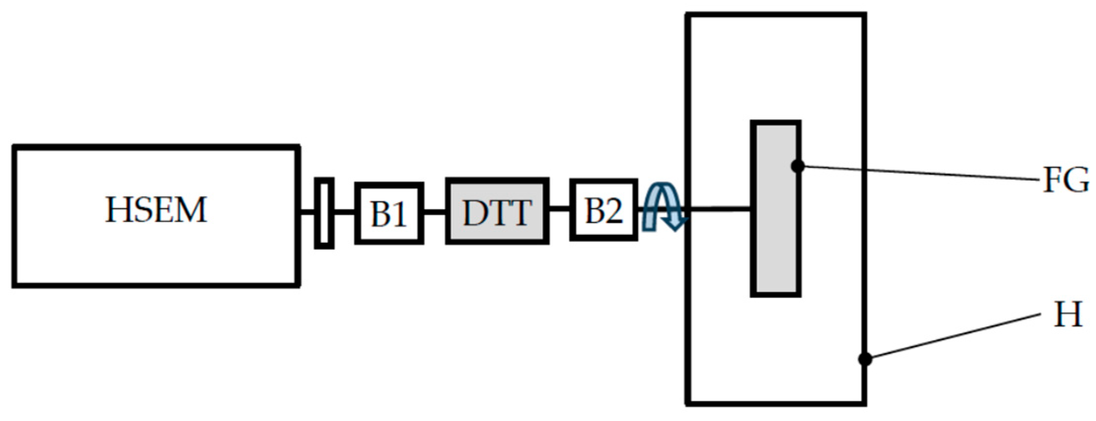
Figure 2.
Variation of the windage torque with rotating speed [14].
Figure 2.
Variation of the windage torque with rotating speed [14].
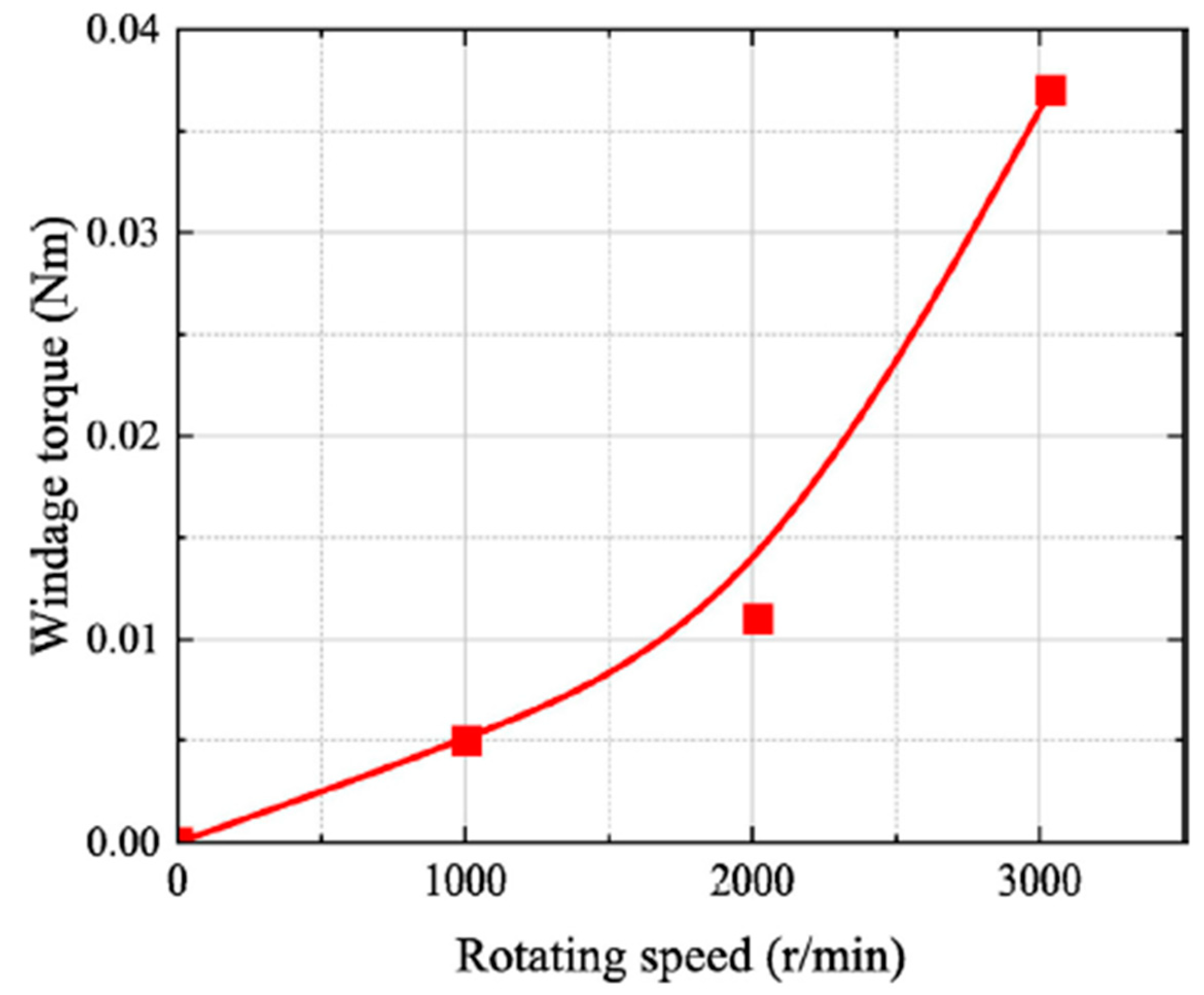
Figure 3.
3D modelling of the test stand (a) Gear geometry; (b) Assembly.
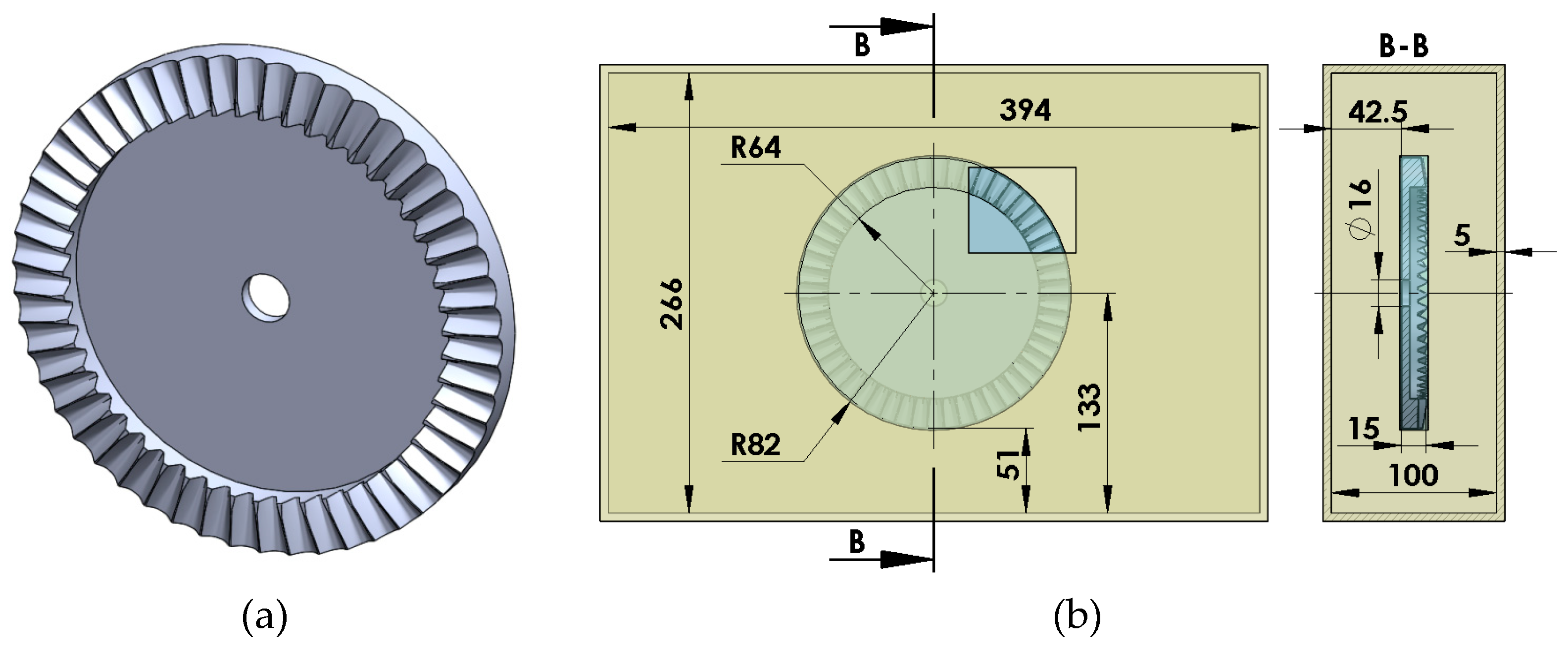
Figure 4.
Flow simulation settings (a) Analysis type; (b) Fluid settings.
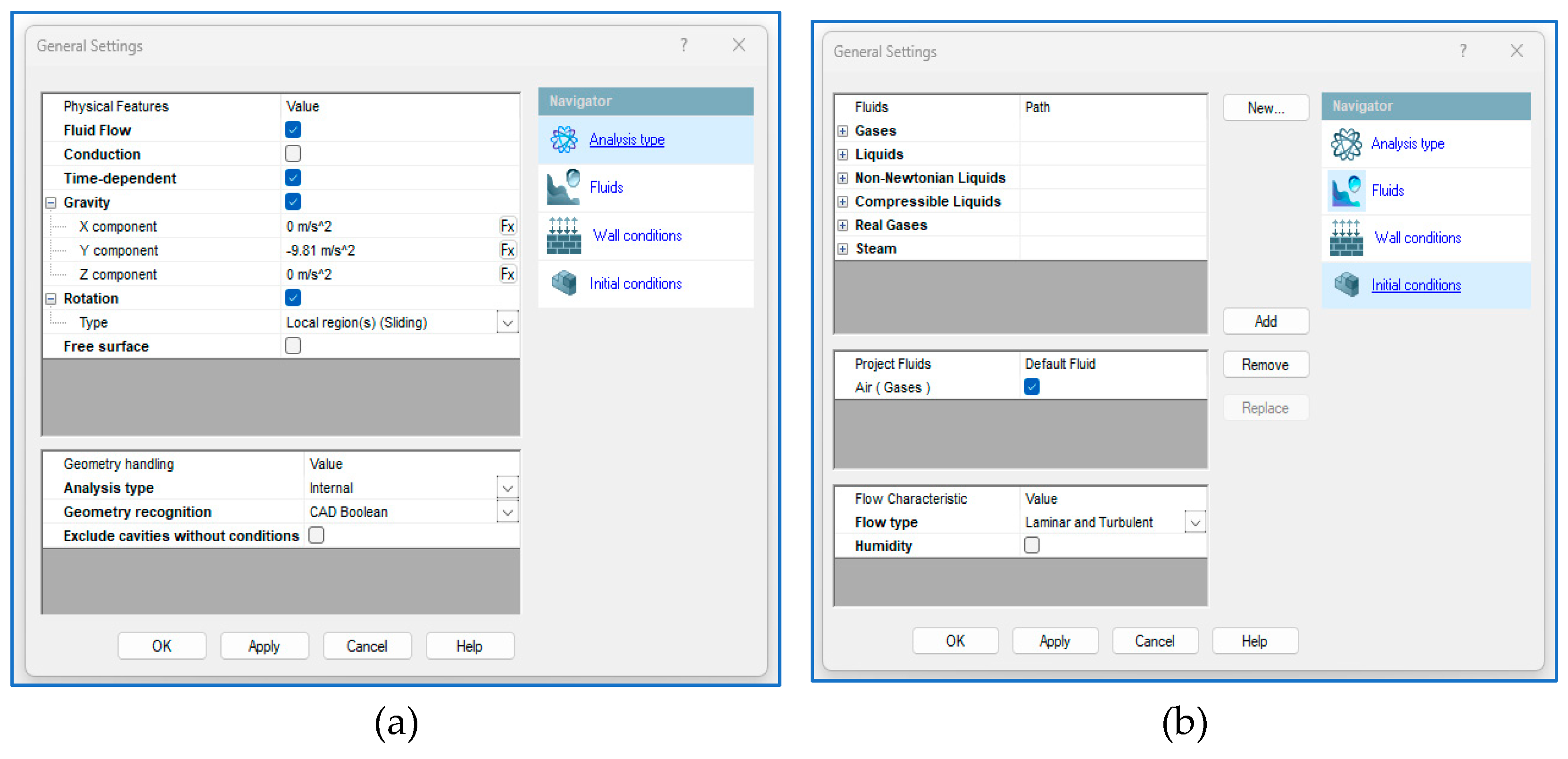
Figure 5.
Rotating Region settings.
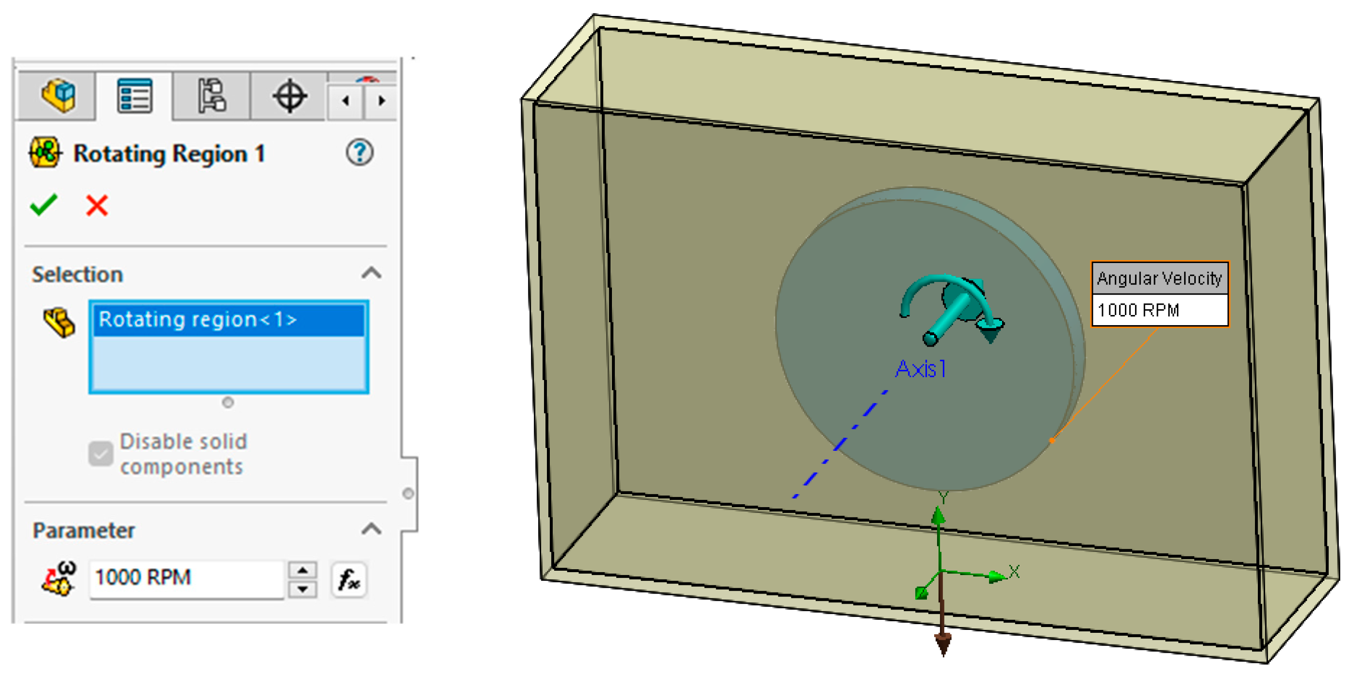
Figure 6.
Computational Domain settings.
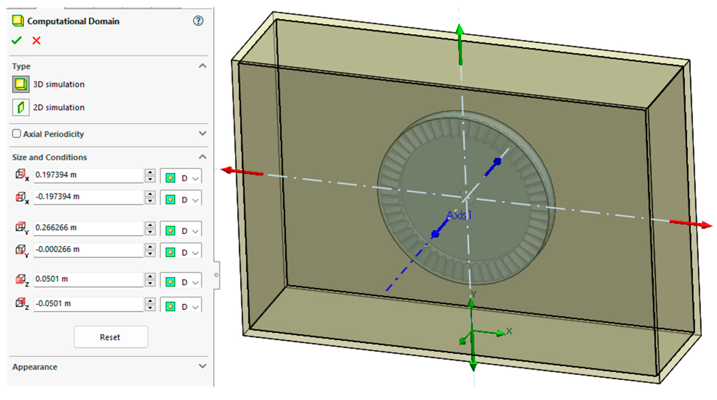
Figure 7.
Gear meshing (a) 35964 cells; (b) 100530 cells; (c) 316775 cells; (d) 689605 cells.
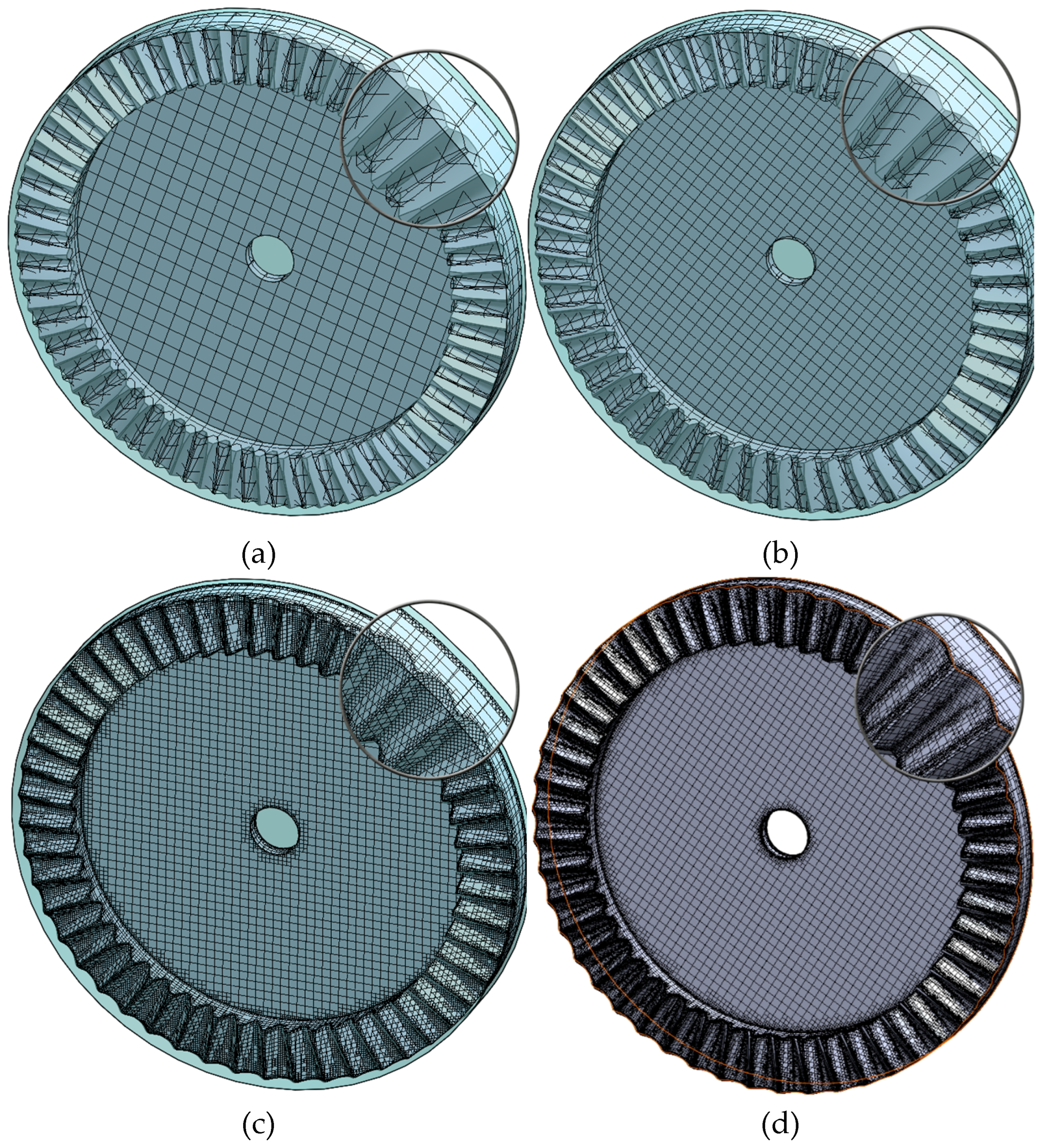
Figure 8.
Result of digitizing the experimentally established variation curve of windage torque.
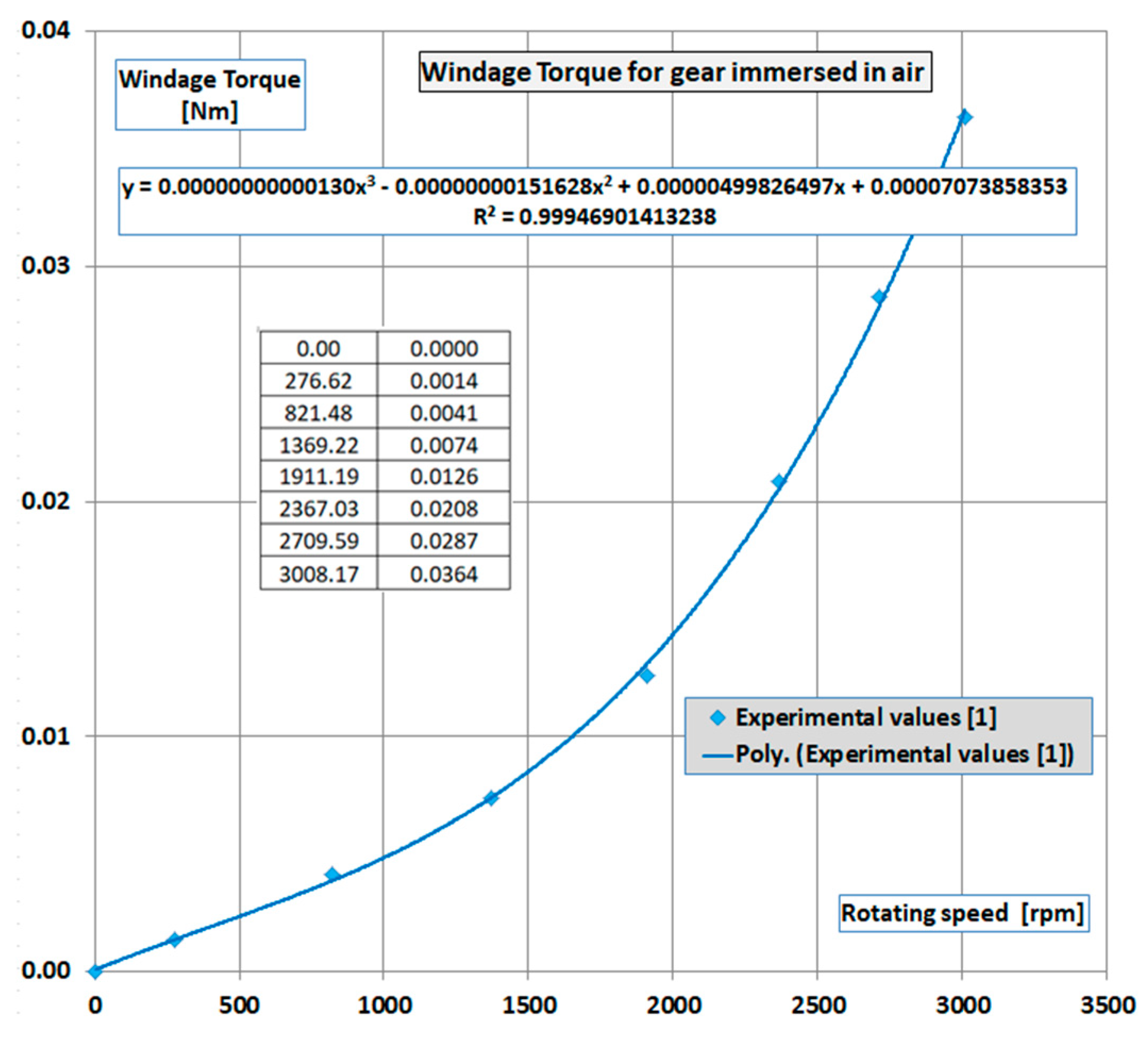
Figure 9.
Comparison of experimental and simulation results.
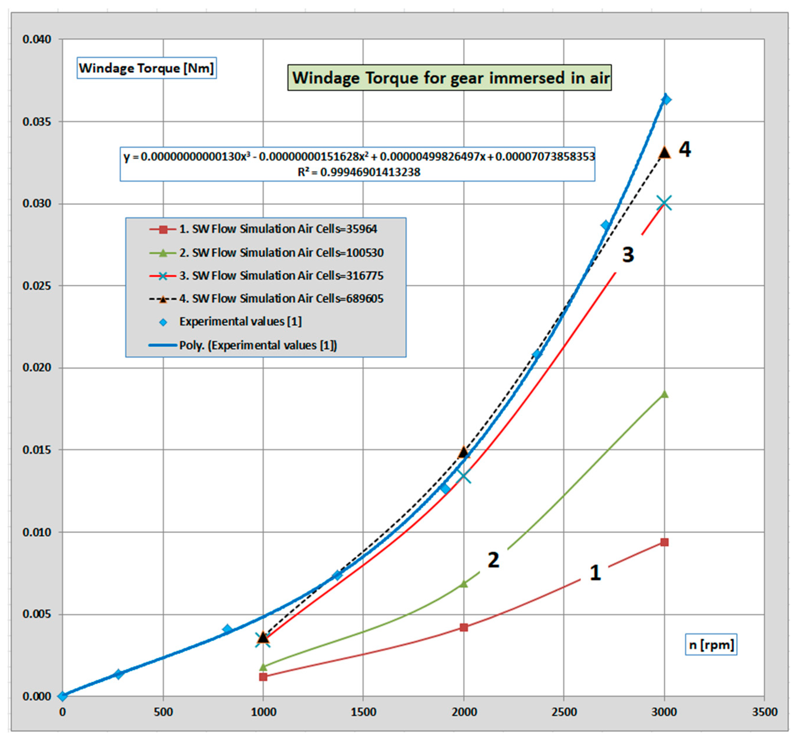
Figure 10.
Convergence chart.
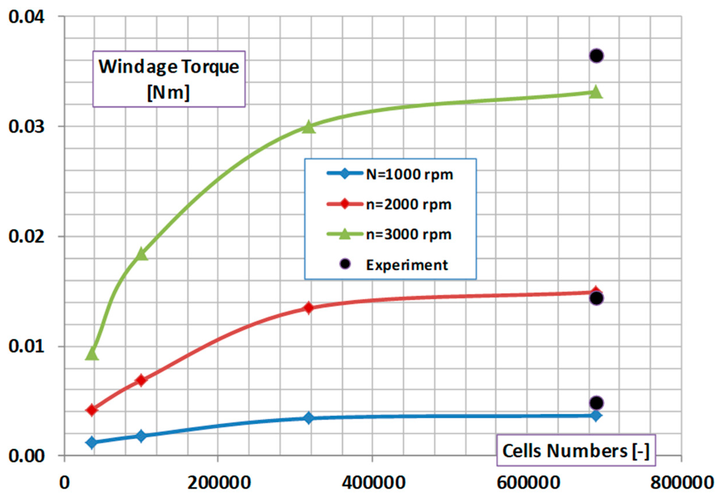
Figure 11.
Influence of mesh refinement on computational resources.
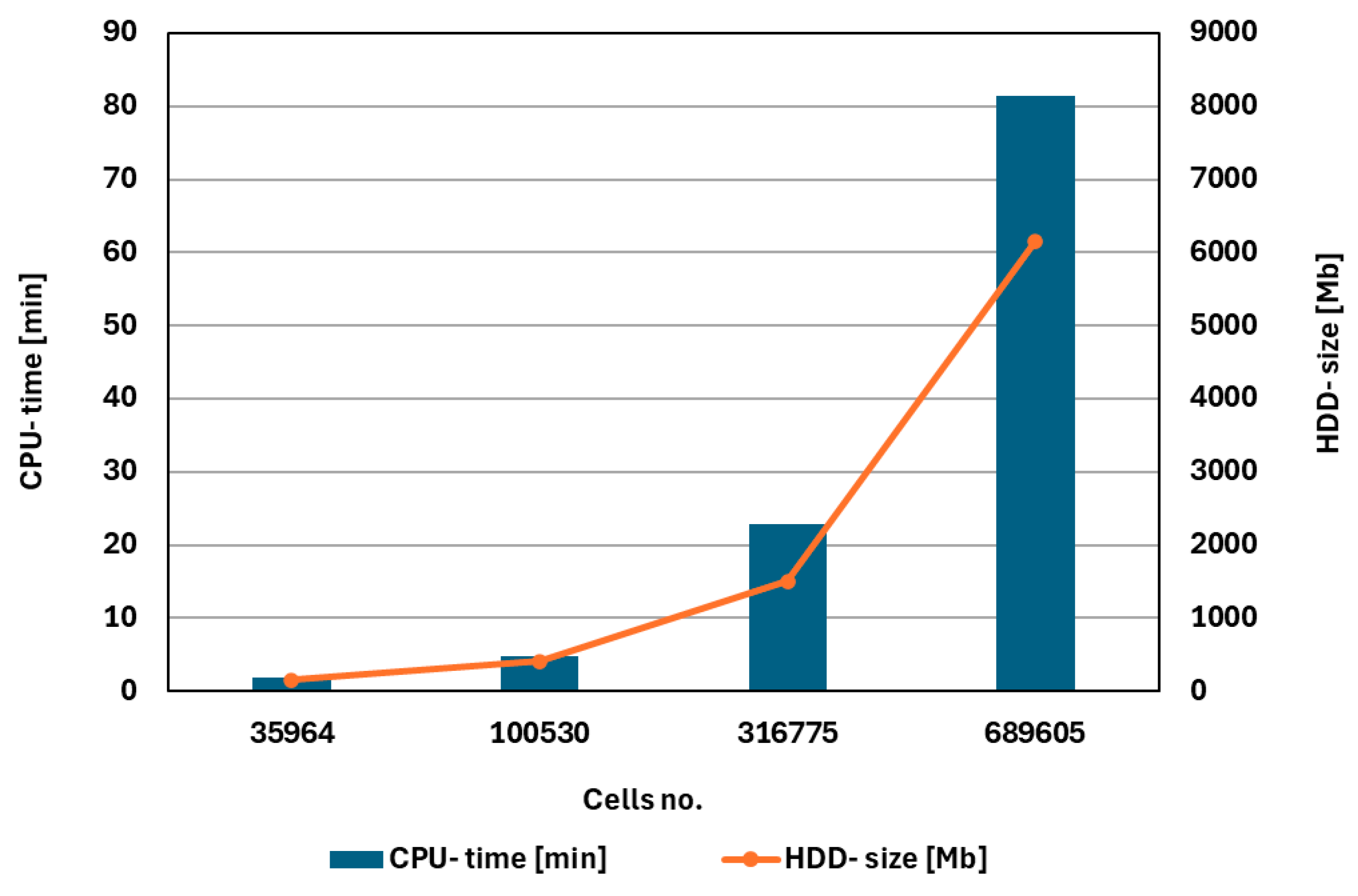
Figure 12.
Velocity distribution in ger front plane.
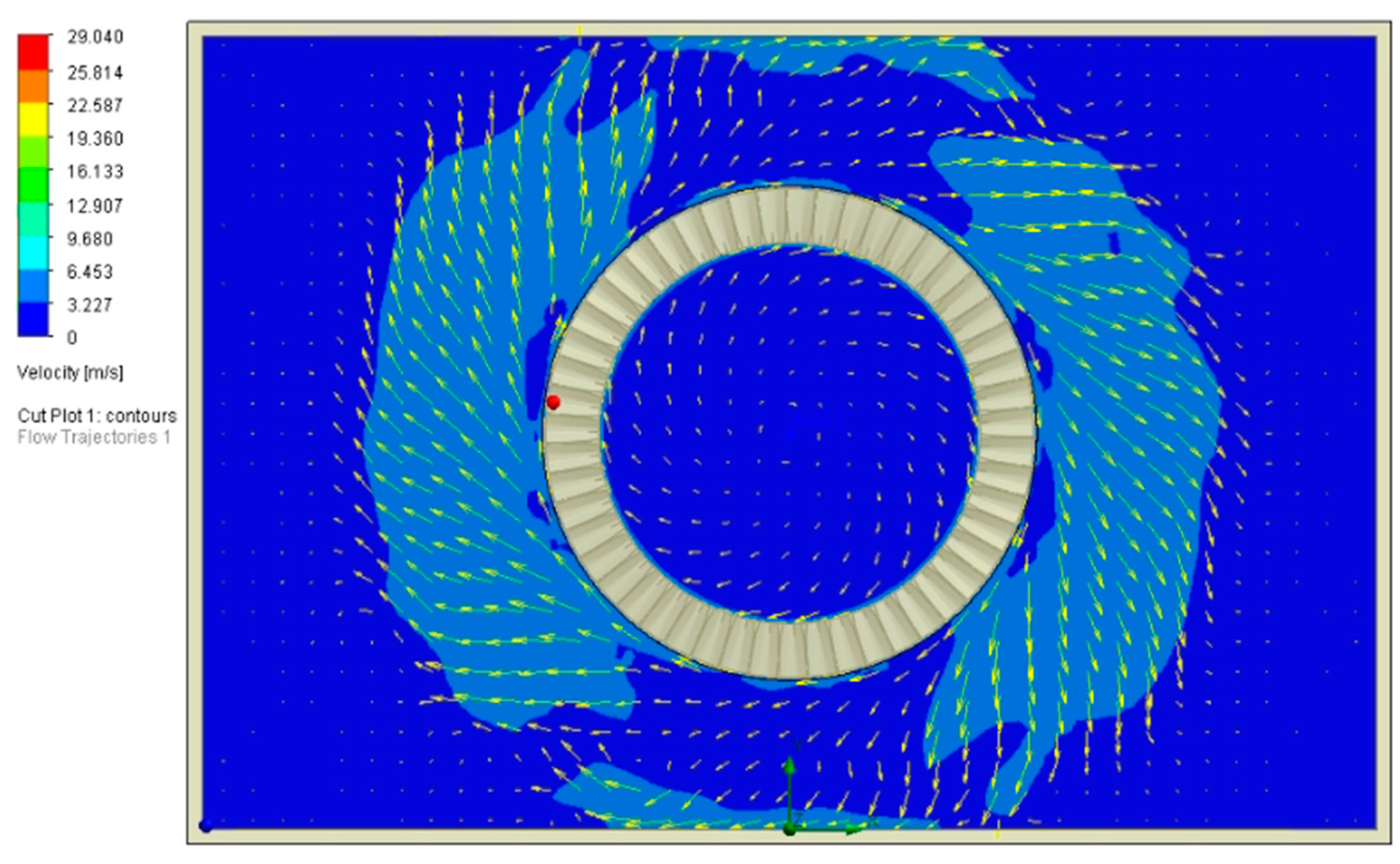
Figure 13.
Flow trajectories inside the gear housing.
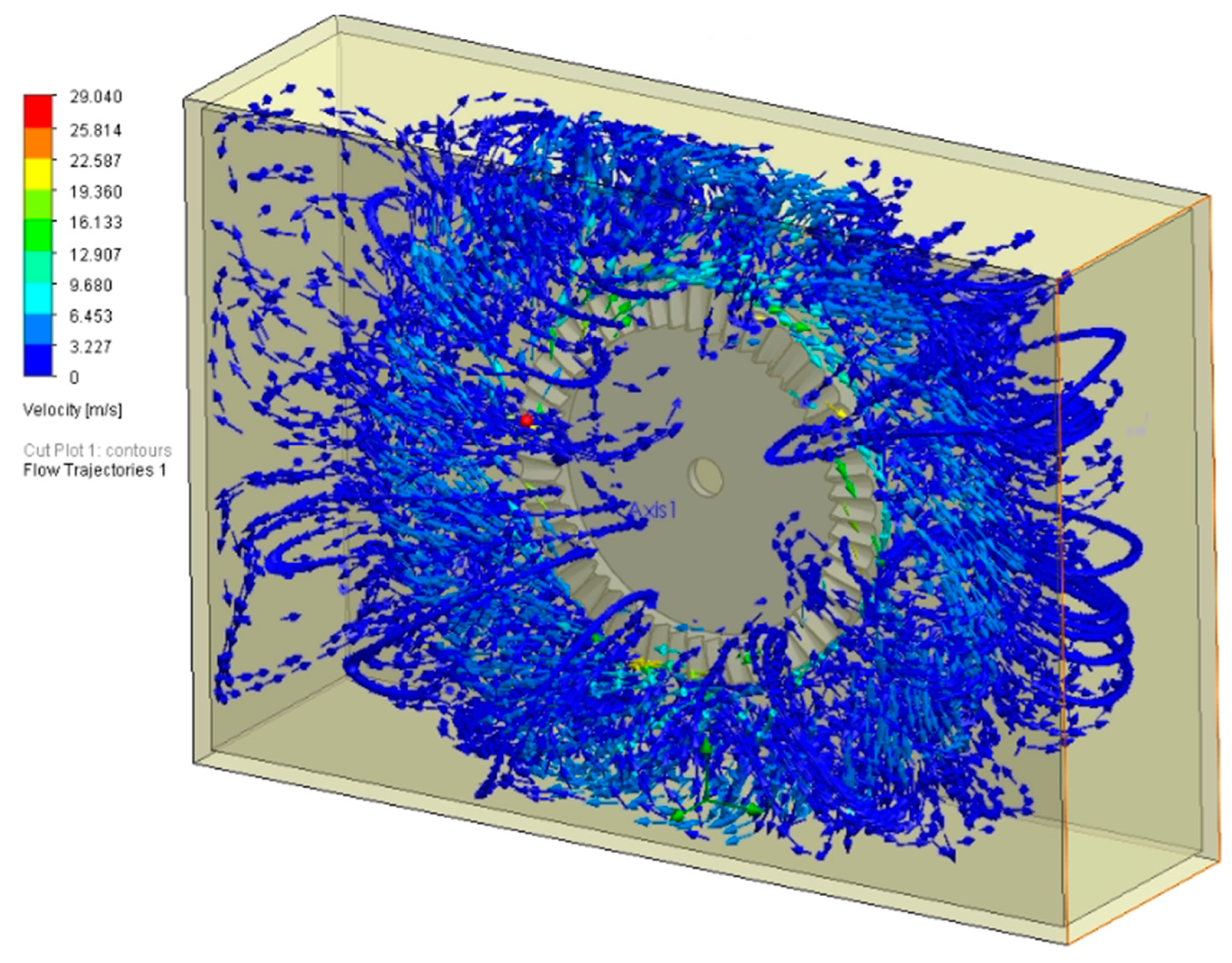

Table 1.
Geometrical parameters of the face gear.
| Parameter | Measurement units | Value |
| Number of teeth | - | 51 |
| Normal module | mm | 2.5 |
| Pressure angle | ° | 25 |
| Inner diameter | mm | 128 |
| Outer diameter | mm | 164 |
Table 2.
General settings of the simulation project.
| Parameter | Setting |
| Fluid flow | activated |
| Time-dependent: | activated, max. time 5 seconds |
| Gravity | activated, 9.81 m/s2 along Y direction |
| Rotation | activated, Local region(s) (Sliding) |
| Analysis type | Internal |
| Geometry recognition | CAD Boolean |
| Exclude cavities without conditions | deactivated |
| Project fluid | Air (Gases) |
| Flow type | Turbulent |
Table 3.
General settings of the simulation project.
| Project no. | Cells no. | Mesh setting | Figure 7 |
| 1 | 35964 | Global mesh: Automatic, level 5 Local mesh: Channels, level 1 Advanced refinement Small Solid Feature Refinement Level: level 1 |
(a) |
| 2 | 100530 | Global mesh: Automatic, level 6 Local mesh: Channels, level 1 Advanced refinement: Small Solid Feature Refinement Level: level 1 |
(b) |
| 3 | 316775 | Global mesh: Automatic, level 7 Local mesh: Channels, level 1 Advanced refinement: Small Solid Feature Refinement Level: level 2 Curvature Level: level 3 |
(c) |
| 4 | 689605 | Global mesh: Automatic, level 7 Local mesh: Channels, level 1 Advanced refinement: Small Solid Feature Refinement Level: level 4 Curvature Level: level 5 |
(d) |
Table 4.
Computer configurations.
| Project no. | Computer configuration |
| 1 | processor12th Gen Intel(R) Core(TM) i5-1240P, 1.70 GHz, 16 cores, installed RAM16.0 GB, 64-bit operating system, x64-based processor |
| 2 | |
| 3 | |
| 4 | processor 11th Gen Intel(R) Core(TM) i9-11900K, 3.50 GHz, 16 cores, installed RAM 64,0 GB, 64-bit operating system, x64-based processor |
Table 5.
Simulation results.
| Project no. | Cells no. | Study no. | Rotating speed [rpm] |
Simulation WT (Nm] |
No. of iterations |
CPU time [min] | HDD Size [Mb] |
| 1 | 35964 | 1.1 | 1000 | 0.0012 | 163 | 1.77 | 167 |
| 1.2 | 2000 | 0.0042 | 163 | 1.83 | 156 | ||
| 1.3 | 3000 | 0.0094 | 163 | 1.90 | 156 | ||
| 2 | 100530 | 2.1 | 1000 | 0.0018 | 230 | 4.90 | 438 |
| 2.2 | 2000 | 0.0069 | 230 | 5.05 | 390 | ||
| 2.3 | 3000 | 0.0184 | 230 | 4.53 | 394 | ||
| 3 | 316775 | 3.1 | 1000 | 0.0034 | 344 | 22.75 | 1490 |
| 3.2 | 2000 | 0.0134 | 360 | 23.60 | 1540 | ||
| 3.3 | 3000 | 0.0300 | 344 | 22.53 | 1480 | ||
| 4 | 689605 | 4.1 | 1000 | 0.0037 | 647 | 87.85 | 6610 |
| 4.2 | 2000 | 0.0149 | 541 | 74.07 | 5650 | ||
| 4.3 | 3000 | 0.0332 | 604 | 82.33 | 6220 |
Table 6.
Differences between experimental and simulation results.
| Rotating speed [rpm] | Digitalized WT [Nm] | Simulation results WT [Nm] / Diff. [%] | |||||||
| 35964 cells | 100530 cells | 316775 cells | 689605 cells | ||||||
| WT | Diff. | WT | Diff. | WT | Diff. | WT | Diff. | ||
| 1000 | 0.0049 | 0.0012 | 75.5 | 0.0018 | 63.3 | 0.0034 | 30.6 | 0.0037 | 24.5 |
| 2000 | 0.0144 | 0.0042 | 70.8 | 0.0069 | 52.1 | 0.0134 | 6.9 | 0.0149 | -3.5 |
| 3000 | 0.0365 | 0.0094 | 74.2 | 0.0184 | 49.6 | 0.0300 | 17.8 | 0.0332 | 9.0 |
| Average Diff. [%] | 73.5 | 55.0 | 18.4 | 10.0 | |||||
Disclaimer/Publisher’s Note: The statements, opinions and data contained in all publications are solely those of the individual author(s) and contributor(s) and not of MDPI and/or the editor(s). MDPI and/or the editor(s) disclaim responsibility for any injury to people or property resulting from any ideas, methods, instructions or products referred to in the content. |
© 2025 by the authors. Licensee MDPI, Basel, Switzerland. This article is an open access article distributed under the terms and conditions of the Creative Commons Attribution (CC BY) license (http://creativecommons.org/licenses/by/4.0/).
Copyright: This open access article is published under a Creative Commons CC BY 4.0 license, which permit the free download, distribution, and reuse, provided that the author and preprint are cited in any reuse.


