
Submitted:
12 March 2025
Posted:
12 March 2025
You are already at the latest version
Abstract
Optimizing the operation of active distribution networks (ADN) has become more challenging because of the uncertainty created by the high penetration level of distributed photovoltaic (PV). From the convex optimization perspective, this paper proposes a two-layer optimization model to simplify the solution of the ADN optimal operation problem. Firstly, to pick out the ADN "key" nodes, a "key" nodes selection approach that used improved K-means clustering algorithm and two indexes (integrated voltage sensitivity and reactive power balance degree) is introduced. Then, a two-layer ADN optimization model is built using various time scales. The upper layer is a long time scale model with on-load tap changer transformer (OLTC) and Capacitor Bank (CB), and the lower layer is a short time scale optimization model with PV inverters and distributed energy storages (ES). To take into account the PV users’ interests, maximizing PV active power output is added to the objective. Afterwards, under the application of the second-order cone programming (SOCP) power flow model, a linearization method of OLTC model and its tap change frequency constraints are proposed. The linear OLTC model, together with the linear models of the other equipment, constructs a mixed-integer second-order cone convex optimization (MISOCP) model. Finally, the effectiveness of the proposed method is verified by solving the IEEE33 node system using the CPLEX solver.
Keywords:
Active distribution networks (ADN)
; Convex optimization
; K-means clustering algorithm
; PV inverter
; Second order cone power flow (SOCP)
1. Introduction
The green and low-carbon transition of energy is the key to realize the “dual-carbon” goals. High penetration level of distributed generators (DG) has led to problems such as node voltage exceeding and power flow reversal, and has posed a huge challenge to power system’s stable and economic operation[1,2,3]. Therefore, it is inevitable to build new power systems[4]. As an important part of the new power system, the distribution network is connected to numerous power electronic devices and has a higher operational complexity. In order to fully leverage the energy and the distribution network’s advantages to cope with the above problems, it is urgent to propose an ADN voltage control strategy with both flexibility and reliability.
PV inverters have the ability of reactive power regulation, which can realize continuous voltage/var control within a certain range. The PV inverters have four kinds of control strategies: maximum active power output control, reactive power control (RPC), active power curtailment (APC) and optimal inverter dispatch (OID)[5,6,7]. The flexible switching of different control strategies can realize the flexible active and reactive power output regulation. In current practical applications, most of the PV inverters use a single control strategy[8], i.e., maximum active power output control, which limits the flexibility of PV inverters regulation. In addition, at some specific times, the PV active power output is too high to be used up, which may result in the resources waste such as abandoned light. Therefore, the PV inverters control strategy that can fully utilize the advantages of multiple control strategies and can take into account the users’ interests is needed.
There are three types of methods for solving the ADN voltage/var control problem: artificial intelligence algorithms (AI), data-driven methods and mathematical methods. However, AI algorithms cannot guarantee the convergence to the global optimum; data-driven algorithms require a large amount of data; mathematical methods, which use solvers to solve problems, are more reliable, but hard to directly solve complex nonlinear problems[9]. The ADN voltage/var control problem is essentially a high-dimensional and high-complex mixed integer nonlinear programming (MINLP) problem which is difficult to solve and needs to be linearized first. By using the second-order cone relaxation, semidefinite relaxation and linear approximation, the Ref. [10,11,12,13] convexified the non-convex power flow model and proposed the SOCP power flow model, the semidefinite programming (SDP) power flow model and the linear approximation (LA) power flow model, respectively. SDP model is more accurate but takes long time to solve; LA model is simple and takes less time but has large errors; the SOCP model is the most widely used one. Ref. [14] proposed a method to linearize the ADN OLTC model by using the big M method under the application of the SOCP power flow model. Although this method can successfully linearize the OLTC model, it requires multiple variable substitutions which increase the linear model complexity and make the model hard to solve. Therefore, a simple linear OLTC model that can be applied under the SOCP power flow model is necessary.
The injected power’s effect on ADN node voltages is different. To fully utilize the compensation devices, it is essential for devices allocation to evaluate the power injection impact on node voltages and select high-impact "key" nodes. Typical indicators used for evaluation are: reactive voltage sensitivity [15], edge weight [16], power transfer distribution factor (PTDF) [17], reactive power balance degree [18], etc. Ref. [19] partitioned the power system based on a comprehensive electrical distance index. Ref. [20] partitioned the distribution networks by using the labeled numbers of the nodes on paths between every two adjacent controllable distributed generations (CDG) as the optimization variables. Power system partitioning usually uses clustering methods, the typical and simple ones are: K-means clustering [21], K-means++ clustering, fuzzy clustering [22], etc. K-means clustering is simple in principle, fast in computation, and feasible in practice. However, for the traditional K-means clustering method, it is sensitive to the initial clustering centers and the selection of initial centers is random. Improper clustering centers can cause problems such as local optimality, slow convergence, and instability. Therefore, when applying the K-means clustering algorithm, the selection of suitable initial clustering centers is very important. In addition, the of the distribution network is relatively low [23,24,25], so it is necessary to consider both active and reactive power effects on the ADN node voltages.
In summary, the key contributions of this paper are as follows:
- Given the single control strategy of PV inverters that restricts reactive power regulation and flexibility, a comprehensive control strategy integrating multiple strategies is proposed. This aims to fully exploit the regulation capacity and account for users’ interests.
- Considering the complex and non - simplified OLTC models under the SOCP power flow model, an OLTC model linearization approach using integers binary expansion and the big M method is proposed. Additionally, a linear model for OLTC tap change frequency constraints is put forward.
- Since current "key" nodes selection indicators in distribution networks mainly focus on reactive power effect while overlooking the active power effect, a comprehensive index encompassing active - reactive voltage sensitivity and reactive power balance degree is proposed.
- Due to the random selection of initial clustering centers in the traditional K - means algorithm, an improved K - means clustering algorithm with an enhanced selection method for initial clustering centers is proposed.
This research was based on the improved IEEE33 case system.
2. Key Nodes Selection
Active-reactive voltage sensitivity and reactive power balance degree constituted the comprehensive evaluation index together. The comprehensive evaluation index and the improved k-means clustering method were used to classify the nodes into “key” ones and “normal” ones.
2.1. Active-Reactive Voltage Sensitivity
The active-reactive voltage sensitivity was obtained by calculating the voltage sensitivity matrix, and the process is shown below.
Let there be a system with n nodes, where there is 1 balanced node, m PV nodes and the others are PQ nodes. In polar coordinate, the power equations for each node of the system are shown in Equation (1) [26].
where, is the active power injection of node i; is the reactive power injection of node i.
Then, based on the Newton-Raphson method, Equation (2) can be derived as follows.
where, J is the Jacobi matrix.
The voltage sensitivity matrix can be obtained by inverting J as shown in Equation (3) [27,28,29].
let and , A and B are the active and reactive voltage sensitivity matrices, respectively. Where, denotes the effect of the node j active change on the node i voltage, i.e., the node i sensitivity to the node j active change. The diagonal elements of matrix describe the voltage sensitivity of the node’s active change to itself; the non-diagonal elements of matrix describe the voltage sensitivity of the node’s active change to others. indicates that increasing the j node active injection can improve the i node voltage stability; indicates that increasing the j node active injection will worsen the i node voltage stability. Reactive voltage sensitivity is the same.
Take the absolute value sum of each node’s active voltage sensitivity and reactive voltage sensitivity. As shown in Equation (4) and Equation (5).
where, N is the set of all nodes.
The comprehensive i node voltage sensitivity can be obtained by normalizing and summing the active and reactive voltage sensitivities, respectively. As shown in Equation (6).
where, and are the weight factors; and are the maximum values of and .
2.2. Reactive Power Balance Degree
The reactive power balance degree was used to describe the level of the node’s reactive power compensation required. The bigger the degree, the higher level of node reactive power compensation required. As shown in Equation (7)[18].
where, is the additional reactive power at node i to qualify the node voltage (0.95 p.u.); is the reactive power supplied to node i in the actual power flow. The formulation of is shown in Equation (2).
where, .
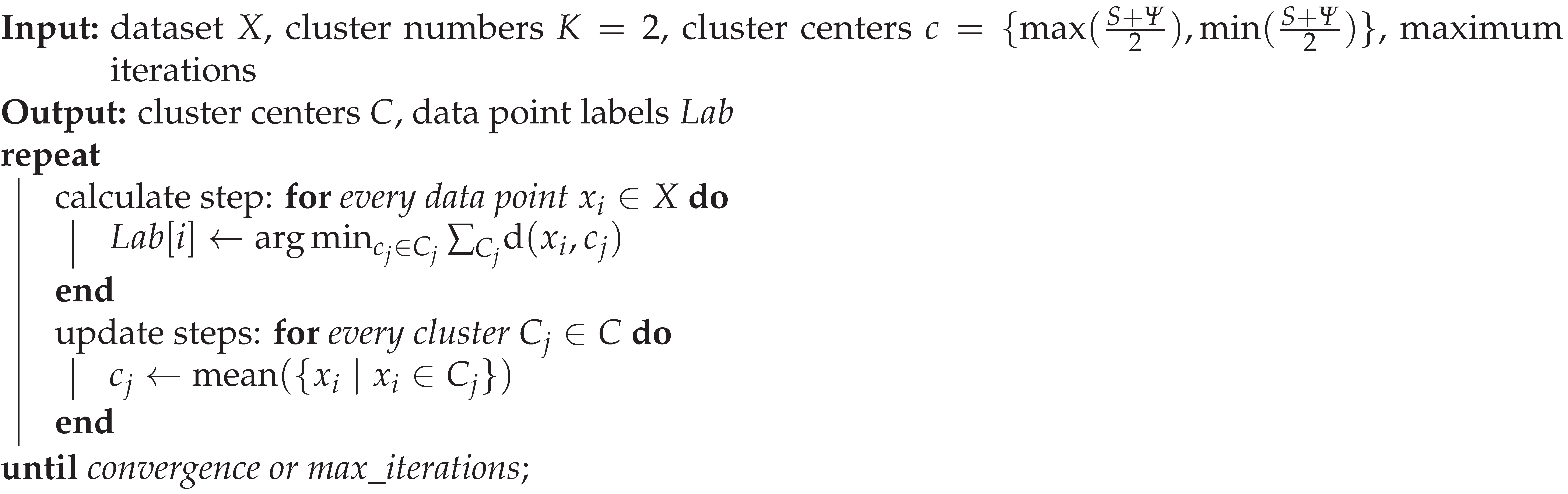
2.3. Node Classification Method Based on Improved K-Means Clustering
The K-means clustering algorithm is one of the most widely used clustering algorithms and also can be used to classify the “key” nodes. The algorithm is simple and useful, but the selection of its clustering number K and initial clustering center directly affects the clustering results[30].
The basic principle of the K-means algorithm is to divide the dataset ( is a d-dimensional vector) into K clusters according to the rule that the sum of squares of all points in the clusters to their clustering centers are the smallest. Each cluster corresponds to a clustering center. As shown in Equation (9).
where, denotes the sample in the ith cluster; denotes the ith cluster’s clustering center.
In this research, the ADN nodes need to be classified into “key” ones and “normal” ones by applying K-means clustering algorithm. Therefore,take .
Since the initial clustering centers of the traditional K-means method are randomly selected, which may lead to slow convergence, the selection way of the initial centers is improved.
The nodes’ active-reactive voltage sensitivities and reactive power imbalance degrees are positively correlated, and it is hoped that the selected "key" nodes have large values of both indexes, so the two points with the largest and smallest indexes mean values were selected as the initial centers. As shown in Equation (10).
The pseudo-code of the improved K-means clustering algorithm is shown in Alg.1.
| Algorithm 1:Improved K-means clustering algorithm. |
 |
3. The Framework of ADN Optimization Operation Model
Let the set of all ADN nodes be N(node 1 is the balanced node), the set of the nodes with PV access be , the set of the nodes with ES access be , the set of the nodes with CB access be , the set of the nodes with OLTC access be , and the set of all lines be L.
3.1. Upper-Layer Optimization Model
In the upper-layer model, the time scale is one hour and the devices are OLTC and CBs.
3.1.1. Upper-Layer Model Constraints
-
Power flow constraintsUsing the branch flow model shown in Figure 1, the branch flow equation shown in Equation (11) is listed according to Ohm’s law, the branch first-end power equation and the node power balance equation.where, ; and are branch ’s transmission power and current; is the injection power of node i, its value is the difference between the power emitted by the generator and the load at node i, i.e., .
-
OLTC modelThe low voltage side of the OLTC is connected to the balancing node. To simplify the model, only the low voltage side of the OLTC is considered. Let the OLTC be an ideal one and set the reference voltage . The OLTC model is shown in Equation (12).where, is the OLTC tap at moment t, the integer variables; is the step size between adjacent taps, its value is 2.5%; K is the total number of taps, its value is 4.
-
CB modelThe CB model is shown in Equation (13).where, is the reactive power compensated by the CB at node j; is the number of CB banks to be switched, the integer variables; is the capacity of each CB bank; is the total number of CB banks connected at node j; is the reactive power consumed by load at node j.
- Node voltage constraintwhere, is the voltage of node i; and are the upper and lower limits of the node i voltage, respectively.
- Branch current constraintwhere, is the maximum current of branch .
3.1.2. Upper-Layer Model Objective Function
The objective function of the upper-layer is the active network loss. According to Ohm’s law, the active network loss is defined as shown in Equation (16).
3.2. Lower-Layer Optimization Model
In the Lower-layer model, the time scale is 30 minutes and the devices are PV inverters and ESs.
3.2.1. Lower-Layer Model Constraints
-
ES modelThe ES model is shown in Equation (17).where, is maximum charging and discharging power of ES; is the capacity of the ES, i.e. the maximum electricity amount that the ES device store; and is the charging and discharging efficiencies, respectively, and ; is the ES charging and discharging state at moment t, 0 denotes charging and 1 denotes discharging; is the ES state of charge (SOC) at the end of moment t,and ; .
-
PV inverter constraintsThe PV inverter constraints are detailed in the lower-layer objective function.
3.2.2. Lower-Layer Objective Function
The lower-layer model considered three objective functions: active network loss, voltage deviation, and user benefits. The first two of them are shown in Equation (18) and Equation (19).
- Active network loss
- Voltage deviation
-
User benefitsThe users benefits are ensured by adjusting PV inverters’ operating strategies. There are two PV inverter control strategies with reactive power regulation capability: RPC and OID. In practical, the operating strategy of PV inverters is maximum active power output control, therefore, the following three control strategies were considered: maximum active power output control, RPC and OID. The principles are shown in Figure 2.The more the PV active power output, the more the users benefits.According to Figure 2, it can be seen that both control strategies (a) and (b) maximize the PV active power output in the current environment, while (c) sacrifices part of the active power output to obtain the reactive power regulation capability. Therefore, making the PV inverter switch along the sequence (a)→(b)→(c) can satisfy the objective of maximizing the PV active power output, i.e., the objective of maximizing the user benefit.In order to obtain the above PV inverters control strategy ((a)→(b)→(c)), the three traditional control strategies were combined and an integrated PV inverters control strategy that balances active power output maximization and reactive power regulation was derived. The integrated strategy is modeled as shown in Equation (23) and Equation (24).where, .
The overall objective function of the lower-layer model is shown in Equation (25).
4. The Convexification of ADN Optimization Operation Model
Convexification of nonlinear models transforms them into simple ones that can be solved directly by the solver. With the application of the SOCP power flow model, the OLTC model is changed into a nonlinear one because of the quadratic term appearance. In addition, the OLTC tap change frequency constraints and ES constraints are also nonlinear.
4.1. The Convexification of Power Flow Model
4.2. The Linearization of OLTC Model
When applying the SOCP power flow model, the OLTC model becomes as shown in Equation (27).
where, is the lower voltage limit of the OLTC secondary side.
Under the application of the SOCP power flow model, the OLTC model becomes nonlinear, therefore, an OLTC linearization method based on binary expansion and big M method was proposed.
First, expand in binary. The total digits is and the value of the s-th digit is , and , as shown in Equation (28).
Then, a new variable is introduced, and . Multiply both sides of by and yield Equation (30).
Afterwards, using the big M method, can be transformed into Equation (31).
where, the M is an arbitrarily large positive number.
Ultimately, the OLTC model is transformed into Equation (32), a mixed integer linear one.
4.3. The Linearization of OLTC Operation Count Constraints
In practice, the OLTC has the limited frequency of tap change throughout the day. OLTC taps cannot be adjusted frequently and each adjustment can only be made between adjacent taps. This creates the strong coupling between time periods for the dynamic voltage/var control problem, which cannot be decoupled into a static one for each time period.
4.4. The Linearization of ES Model
From Equation (17), it can be seen that the charging and discharging of the ESs cannot be performed simultaneously. This lead to nonlinear constraints for both the charging and discharging power constraints and the SOC constraints.
-
ES power constraints
-
ES SOC constraintsThe original ESs SOC constraints are shown in Equation (37). Using the big M method can linearize it. The linearized constraints is shown in Equation (38).The Equation (39) constraints enable that in the charging state (), only the charge SOC is valid while the discharge SOC is not; and in the discharging state (), only the discharge SOC is valid while the charge SOC is not.
5. Case Study
IEEE33 node radial distribution network and Matlab 2022b were used in the case study.
5.1. "Key" Nodes Selection
The results of "key" nodes selection are shown in Figure 3, the red dots indicate "key" nodes, the blue dots indicate "normal" nodes, and the asterisks are the clustering centers. It can be seen that the improved K-means clustering algorithm has a good classification effect. The "key" nodes are: 6, 7, 8, 9, 10, 11, 12, 13, 14, 15, 16, 18, 25, 26, 27, 28, 29, 30, 31, 32.
5.2. Case Allocation
Using the IEEE33 distribution network system, referring to the above key nodes and based on the experience, the case allocation is: Configure PV according to high penetration situation. The number of the PVs is two, both capacities are 1800kW, the total capacity is 3600kW, connected to node 18 and node 31, respectively. The number of the CBs is two, connected to node 10 and node 29 respectively and their capacities are 1300kVar and 1000kVar respectively. Both CBs have 10 banks and each bank’s capacities are 130kVar and 100kVar, respectively. The OLTC is connected to node1.It has 5 taps, the step between two taps is 2.5%, so, the OLTC voltage regulation range is 0.95-1.05p.u.. The number of the distributed ESs is two, connected to node 18 and node 31 respectively ,their capacities are both 13MW and their maximum charging and discharging power are both 1.7MW.
The case allocation is in Figure 4.
5.3. Curves for Load and PV Active Power Output
The 24-hour active and reactive load curves are shown in Figure 5, and their projections demonstrate the trend of their values over time and over nodes. From the figures, it can be seen that the active load connected to node 24 is maximum while the reactive load connected to node 30 is maximum. During the day, there are two peaks for both active and reactive loads, the two peaks for active loads are at the 14 and 21 moments respectively, and the two peaks for reactive loads are at the 13 and 20 moments respectively.
The 24-hour original PV active power output curve (each PV) is shown in Figure 6.
It can be seen that the peak PV active power output moment is around 13 moment, and there are about 9 hours in a day when the PV active power output is zero.
5.4. Upper-Layer Equipment Dispatching Strategies
The OLTC dispatching strategy is shown in Figure 7.
It can be seen from the figure, the low voltage side voltages of the OLTC is in the range of 0.975p.u.-1.025p.u. and lies between the lower limit of 0.95p.u. and the upper limit of 1.05p.u.. The number of tap adjustments in a day is 6. Tap adjustments between adjacent moments are continuous, and tap adjustments between the 1 and 24 moments are also continuous. All of them meet the OLTC operation requirements.
The dispatching strategy of the two CBs are shown in Figure 8.
It can be seen that the first compensation small peak occurs around 11 moment and the second compensation small peak occurs around 16 moment. This is because the load is high at these two moments and the reactive power compensation is increased to ensure that the voltages are within the qualified range.
5.5. Lower-Layer Equipment Dispatching Strategies
The generator active power output curve of the day at the first end of ADN is shown in Figure 9.
It can be seen that the generator active output has two peaks near 13 moment and 20 moment respectively, roughly coinciding with the two peak moments of the load curve. The ADN system does appears the reverse power flow due to excess PV generation, so there is no negative power in the generator. This satisfies the conditions for proper ADN system operation.
The dispatching strategies for ESs are shown in Figure 10.
It can be seen that at peak moments the ESs discharge to meet load demand; the rest of the time they charge.
The PVs reactive power output dispatching strategies are shown in Figure 11.
It can be seen that the PVs curve of reactive power output is similar to the CBs reactive power output. Both of them have two peaks near 13 moment and 20 moment, which is due to meet the load demand while satisfying the voltage qualification.
The PVs’ active power output of the day before and after dispatching is shown in Figure 12.
It can be seen that before and after dispatching, the active power output of the PVs is almost unchanged. This is the result of pursuing the maximum PVs active output to ensure the users’ interests. Therefore, the results of the dispatching are satisfactory.
5.6. Optimal Dispatching Results
The network loss before optimal dispatching is 1.355MW, and the network loss after optimal dispatching is 336.077kW, decreased by 75.20%. It shows that the optimization effect for network loss is obvious.
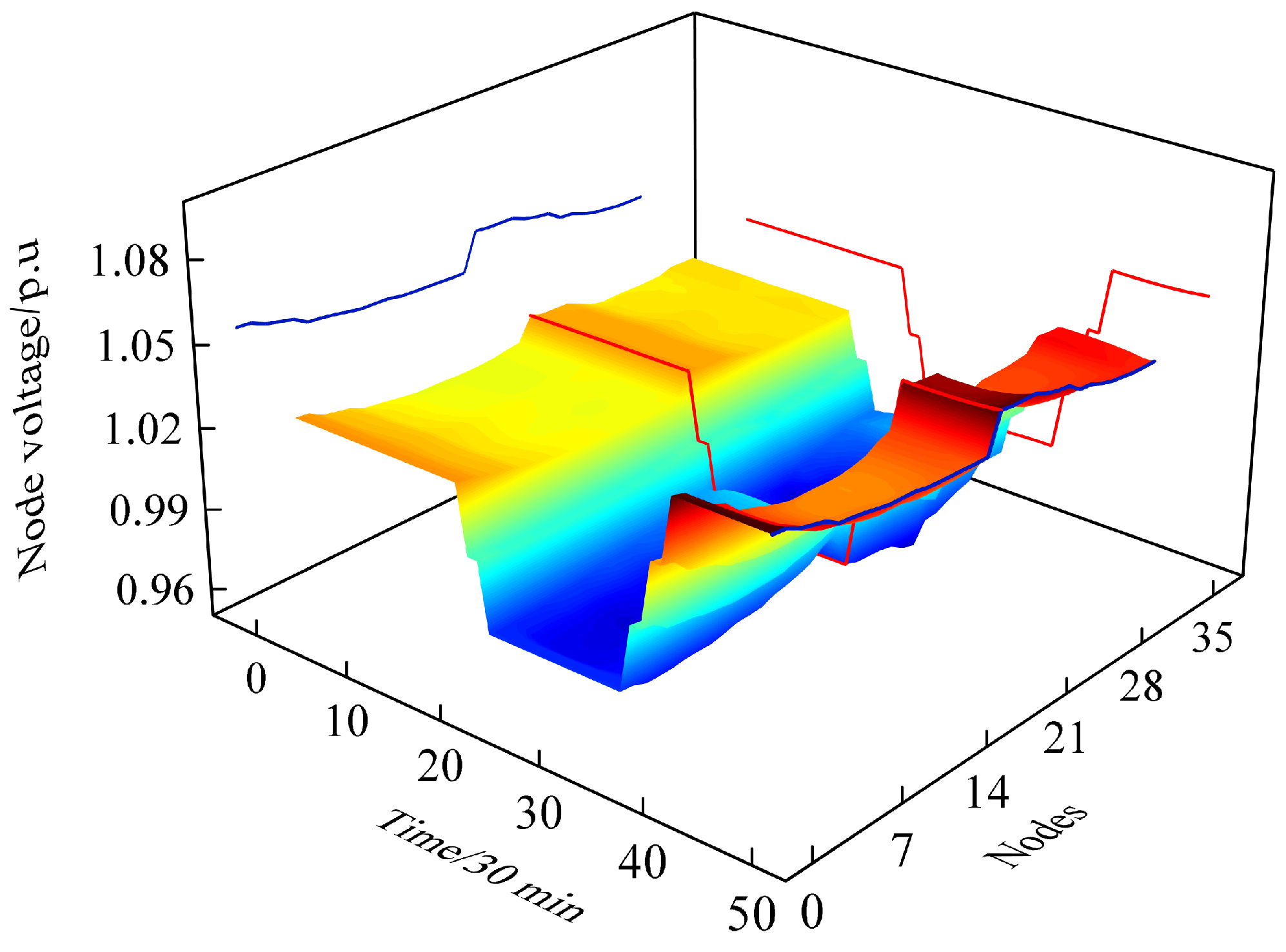
The node voltages of the ADN are shown in the Figure 13, and its projections show the trend of voltage values over time and over nodes.
It can be seen that the all node voltages specification is between 0.95 p.u. and 1.05 p.u., which are all within the qualified range. In addition, from the perspective of time, it also can be seen that the trend of the node voltages is the same as that of OLTC. This means that the OLTC has a great influence on the node voltages.
6. Conclusions
In order to solve the problem of ADN increased dispatching difficulty caused by the high DG penetration, this paper proposed a two-layer optimal dispatching model for ADN based on convex optimization. Firstly, the active-reactive voltage sensitivity and reactive power balance degree were introduced as comprehensive indexes, and the "key" nodes were selected using the improved K-means clustering method. Then, a two-layer optimization model was established based on the different time scales. The upper-layer model is a long time scale one, contains OLTC and CBs. The lower-layer model is a short time scale one, contains PV inverters and ESs. In addition, by proposing the PV inverters’ comprehensive control strategy, the model also took into account the users’ benefits. Afterwards, the linearization methods were proposed for OLTC model and its operation constraints model, and the two-layer model was eventually transformed into a MISOC model. Finally, the effectiveness of the proposed method was verified by solving the improved IEEE33 case using the CPLEX solver and the following conclusions were drawn:
- the proposed OLTC linearization method did simplify the OLTC model under the application of the SOCP power flow mode. And the proposed OLTC tap change frequency constraints linearization method made the OLTC model more practical;
- the proposed PV inverters control strategy enabled voltage/var control while simultaneously ensuring user benefits;
- the proposed comprehensive "key" node selection indexes and the proposed improved K-means algorithm increased the reliability of key node selection;
- the proposed two-layer optimization model has led to a 70% reduction in network losses and has successfully maintained all node voltages within qualified limits. This demonstrates tmahat the proposed method is beneficial for both the economic and stable operation of the distribution network.
References
- Mehrjerdi, H.; Hemmati, R.; Farrokhi, E. Nonlinear stochastic modeling for optimal dispatch of distributed energy resources in active distribution grids including reactive power. Simulation Modelling Practice and Theory 2019, 94, 1–13. [Google Scholar] [CrossRef]
- Kerrouche, S.; Djerioui, A.; Zeghlache, S.; Houari, A.; Saim, A.; Rezk, H.; Benkhoris, M.F. Integral backstepping-ILC controller for suppressing circulating currents in parallel-connected photovoltaic inverters. Simulation Modelling Practice and Theory 2023, 123, 102706. [Google Scholar]
- Song, J.; Jung, S.; Lee, J.; Shin, J.; Jang, G. Dynamic performance testing and implementation for static var compensator controller via hardware-in-the-loop simulation under large-scale power system with real-time simulators. Simulation Modelling Practice and Theory 2021, 106, 102191. [Google Scholar] [CrossRef]
- Jingjing, W.; Liangzhong, Y.; Jun, L.; Jun, W.; Fan, C. Distributed optimization strategy for networked microgrids based on network partitioning. Applied Energy 2025, 378, 124834. [Google Scholar]
- Tao, D.; Cheng, L.; Yongheng, Y.; Jiangfeng, J.; Zhaohong, B.; Frede, B. A two-stage robust optimization for centralized-optimal dispatch of photovoltaic inverters in active distribution networks. IEEE Transactions on Sustainable Energy 2016, 8, 744–754. [Google Scholar]
- Emiliano, D.; Sairaj, V.; Brian, G.; Georgios, B. Optimal dispatch of residential photovoltaic inverters under forecasting uncertainties. IEEE Journal of Photovoltaics 2014, 5, 350–359. [Google Scholar]
- Emiliano, D.; Sairaj, V.; Brian, G.; Georgios, B. Decentralized optimal dispatch of photovoltaic inverters in residential distribution systems. IEEE Transactions on Energy Conversion 2014, 29, 957–967. [Google Scholar]
- González-Moreno, A.; Marcos, J.; Parra, I.; Marroyo, L. Control method to coordinate inverters and batteries for power ramp-rate control in large PV plants: Minimizing energy losses and battery charging stress. Journal of Energy Storage 2023, 72, 108621. [Google Scholar] [CrossRef]
- Lizi, L.; Wei, G.; Xiaoping, Z.; Ge, C.; Weijun, W.; Gang, Z.; Dingjun, Y.; Zhi, W. Optimal siting and sizing of distributed generation in distribution systems with PV solar farm utilized as STATCOM (PV-STATCOM). Applied Energy 2018, 210, 1092–1100. [Google Scholar]
- Masoud, F.; Steven H, L. Branch flow model: Relaxations and convexification—Part I. IEEE Transactions on Power Systems 2013, 28, 2554–2564. [Google Scholar]
- Masoud, F.; Steven H, L. Branch flow model: Relaxations and convexification—Part II. IEEE Transactions on Power Systems 2013, 28, 2565–2572. [Google Scholar]
- Zeyu, W.; Daniel S, K.; Baosen, Z. Accurate semidefinite programming models for optimal power flow in distribution systems. arXiv, 2017; arXiv:1711.07853. [Google Scholar]
- Lingwen, G.; Steven H, L. Convex relaxations and linear approximation for optimal power flow in multiphase radial networks. In Proceedings of the 2014 power systems computation conference; 2014; pp. 1–9. [Google Scholar]
- Wenchuan, W.; Zhuang, T.; Boming, Z. An exact linearization method for OLTC of transformer in branch flow model. IEEE Transactions on Power Systems 2016, 32, 2475–2476. [Google Scholar]
- Ketian, Y.; Junbo, Z.; Can, H.; Nan, D.; Yingchen, Z.; Thomas E, F. A data-driven global sensitivity analysis framework for three-phase distribution system with PVs. IEEE Transactions on Power SystemsIEEE Transactions on Power Systems 2021, 36, 4809–4819. [Google Scholar]
- Rubén J, S.; Max, F.; Seán, N.; Nick, W.; Graham, N.; Jacek, B.; Janusz W, B. Hierarchical spectral clustering of power grids. IEEE Transactions on Power Systems 2014, 29, 2229–2237. [Google Scholar]
- Di, S.; Daniel J, T. A novel bus-aggregation-based structure-preserving power system equivalent. IEEE Transactions on Power Systems 2014, 30, 1977–1986. [Google Scholar]
- Bo, Z.; Zhicheng, X.; Chen, X.; Caisheng, W.; Feng, L. Network partition-based zonal voltage control for distribution networks with distributed PV systems. IEEE Transactions on Smart Grid 2017, 9, 4087–4098. [Google Scholar]
- Lingzhuochao, M.; Xiyun, Y.; Jiang, Z.; Xinzhe, W.; Xin, M. Network partition and distributed voltage coordination control strategy of active distribution network system considering photovoltaic uncertainty. Applied Energy 2024, 362, 122846. [Google Scholar]
- Li, M.; Lingfeng, W.; Zhaoxi, L. Self-organized partition of distribution networks with distributed generations and soft open points. Electric Power Systems Research 2022, 208, 107910. [Google Scholar]
- Yiming, L.; Che, L.; Lizhi, Z.; Bo, S. A partition optimization design method for a regional integrated energy system based on a clustering algorithm. Energy 2021, 219, 119562. [Google Scholar]
- Yi, W.; Jiahao, M.; Ning, G.; Qingsong, W.; Liang, S.; Hongye, G. Federated fuzzy k-means for privacy-preserving behavior analysis in smart grids. Applied Energy 2023, 331, 120396. [Google Scholar]
- Zhu, Z.; Zeng, F.; Qi, G.; Li, Y.; Jie, H.; Mazur, N. Power system structure optimization based on reinforcement learning and sparse constraints under DoS attacks in cloud environments. Simulation Modelling Practice and Theory 2021, 110, 102272. [Google Scholar] [CrossRef]
- Manzoor, A.; Judge, M.A.; Ahmed, F.; ul Islam, S.; Buyya, R. Towards simulating the constraint-based nature-inspired smart scheduling in energy intelligent buildings. Simulation Modelling Practice and Theory 2022, 118, 102550. [Google Scholar]
- Suryakiran, B.; Nizami, S.; Verma, A.; Saha, T.; Mishra, S. A DSO-based day-ahead market mechanism for optimal operational planning of active distribution network. Energy 2023, 282, 128902. [Google Scholar]
- Yue, X.; Yu, L.; Junyong, L. Deep reinforcement learning based topology-aware voltage regulation of distribution networks with distributed energy storage. Applied Energy 2023, 332, 120510. [Google Scholar]
- Miguel, P.; Lukas, O.; Saverio, B.; Florian, D. Adaptive real-time grid operation via online feedback optimization with sensitivity estimation. Electric Power Systems Research 2022, 212, 108405. [Google Scholar]
- Jochen, S.; Thierry, Z.; Giacomo, P.; Damiano, T.; Gabriela, H.; Konstantinos, B. Sensitivity analysis of electric vehicle impact on low-voltage distribution grids. Electric Power Systems Research 2021, 191, 106696. [Google Scholar]
- Georgia, P.; Xiaozhe, W. An online network model-free wide-area voltage control method using PMUs. IEEE Transactions on Power Systems 2021, 36, 4672–4682. [Google Scholar]
- González-Cabrera, N.; Ortiz-Bejar, J.; Zamora-Mendez, A.; Paternina Mario R, A. On the Improvement of representative demand curves via a hierarchical agglomerative clustering for power transmission network investment. Energy 2021, 222, 119989. [Google Scholar]
Figure 1.
The branch flow diagram.
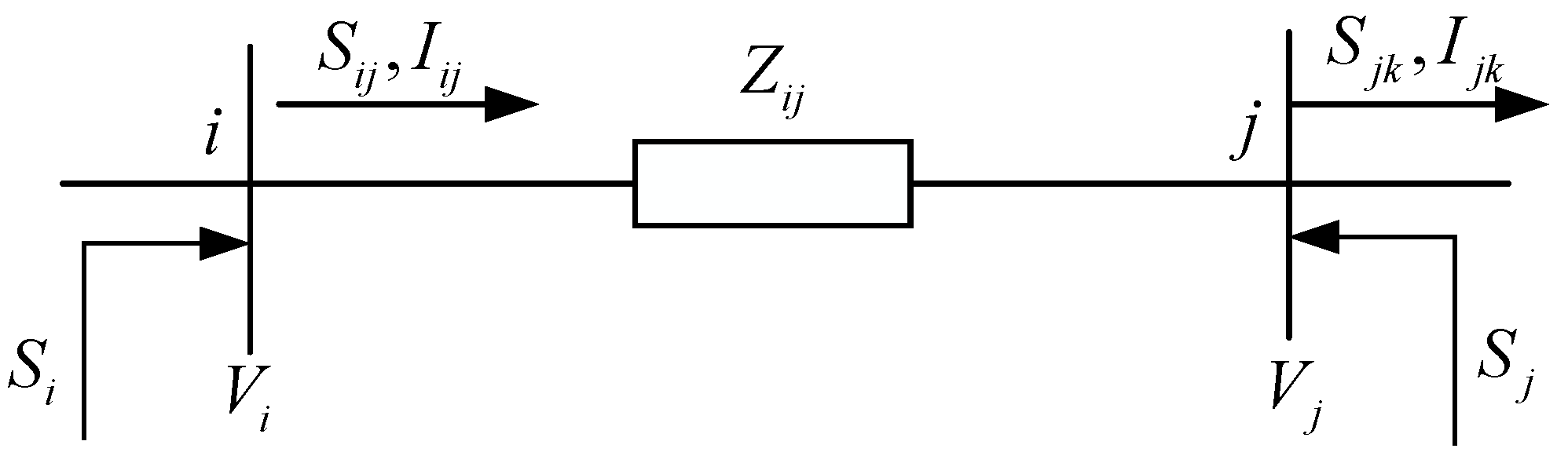
Figure 2.
PV inverter’s three control strategies .(a) Maximum active power output control. (b) RPC. (c) OID.
Figure 2.
PV inverter’s three control strategies .(a) Maximum active power output control. (b) RPC. (c) OID.
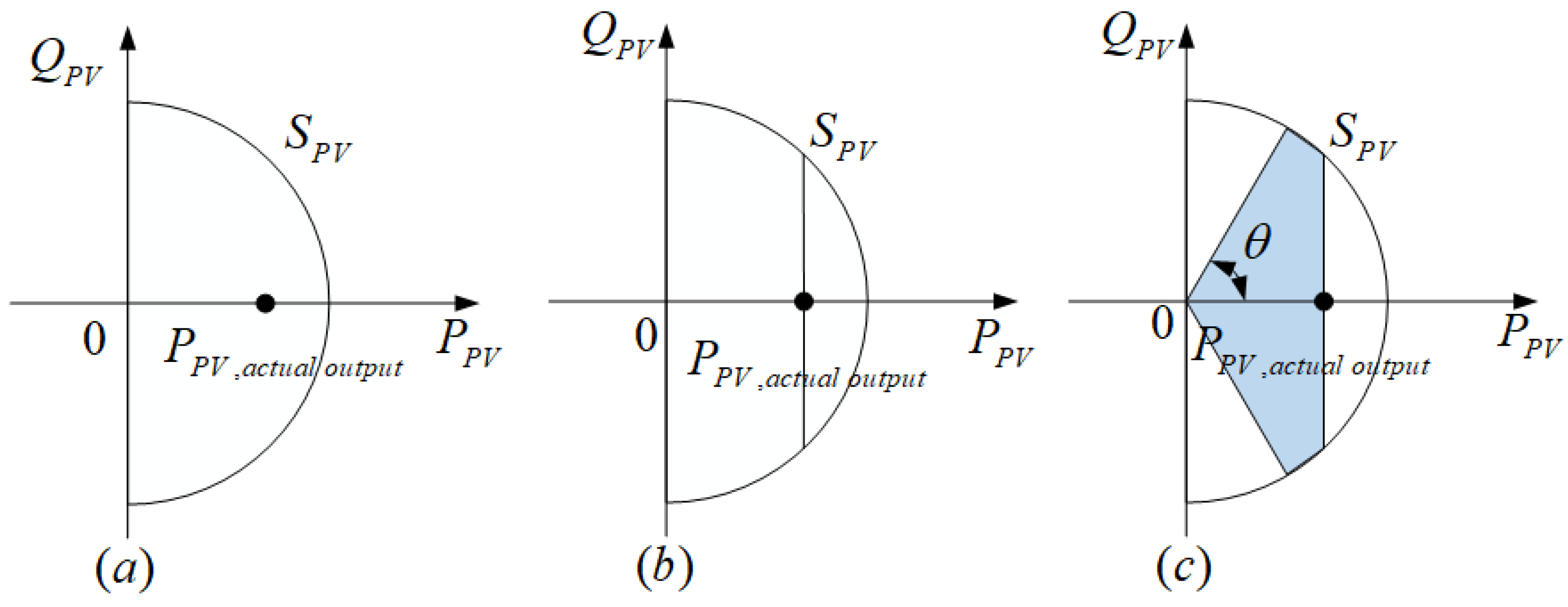
Figure 3.
"Key" nodes selection results.
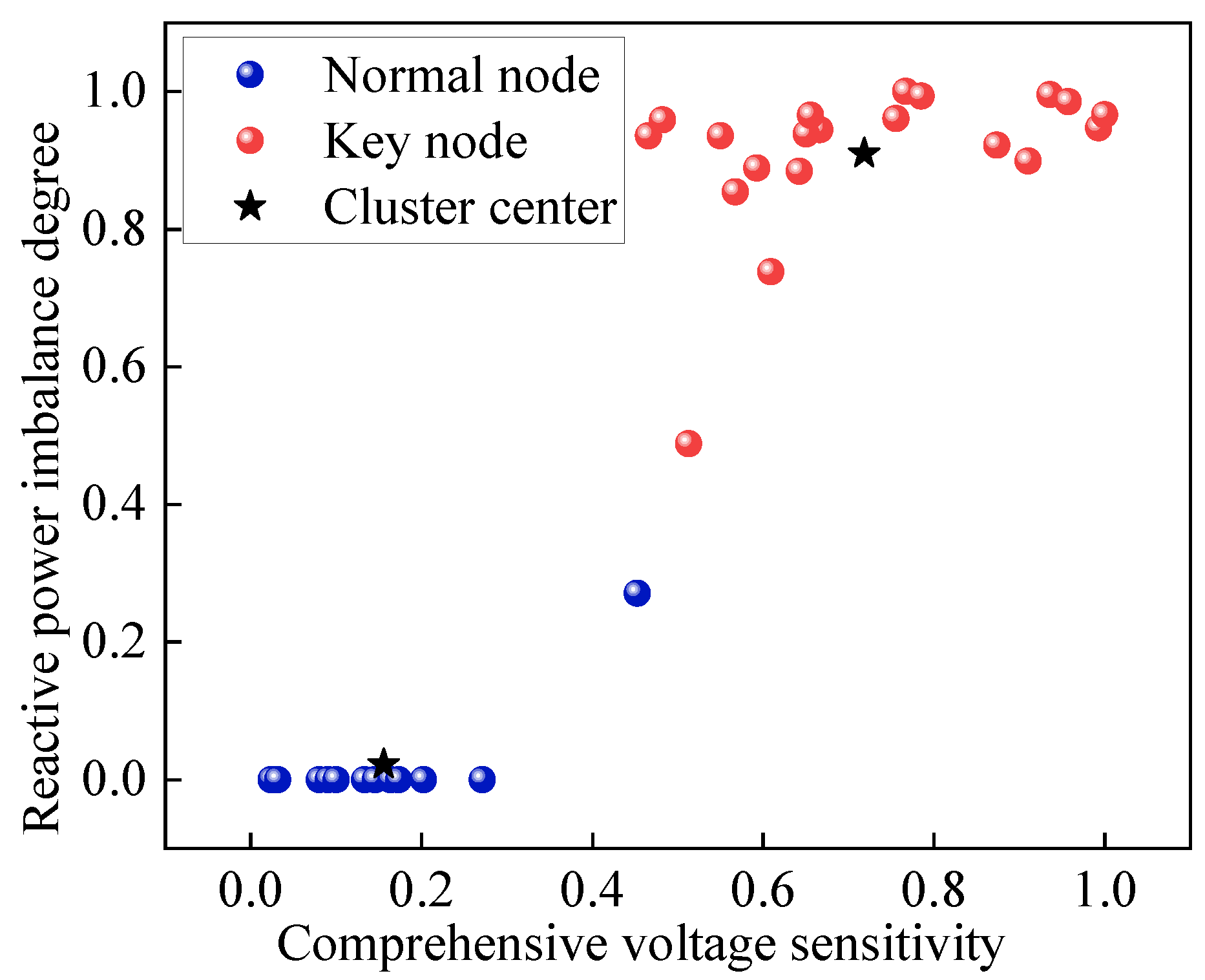
Figure 4.
Case configuration.
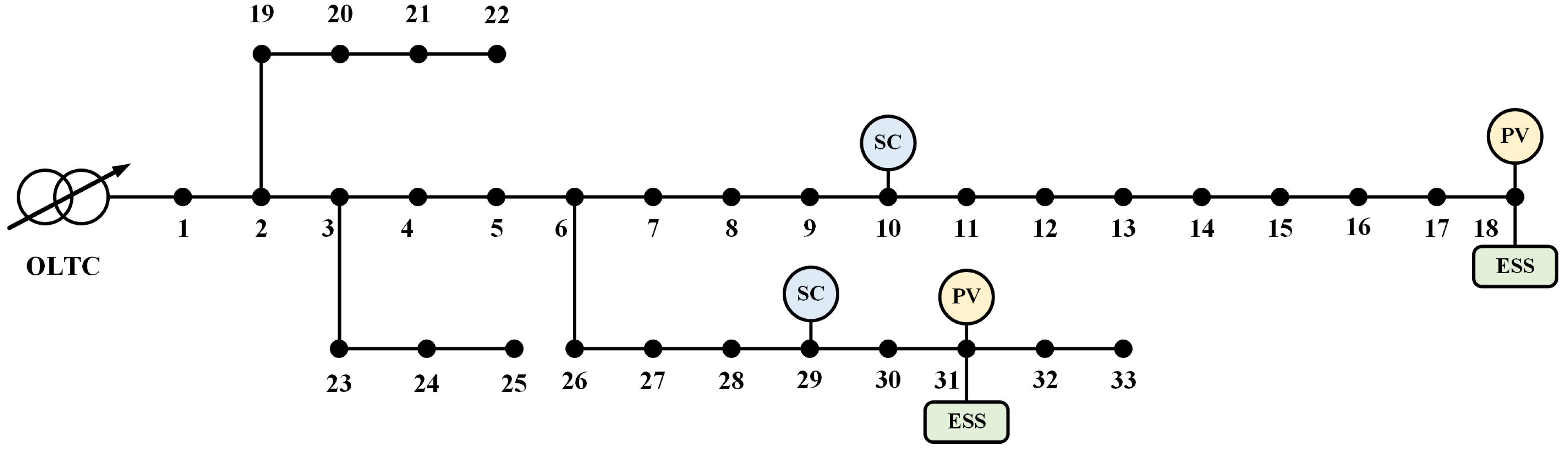
Figure 5.
24-hour load curve. (a) 24-hour active load curve. (b) 24-hour reactive load curve.
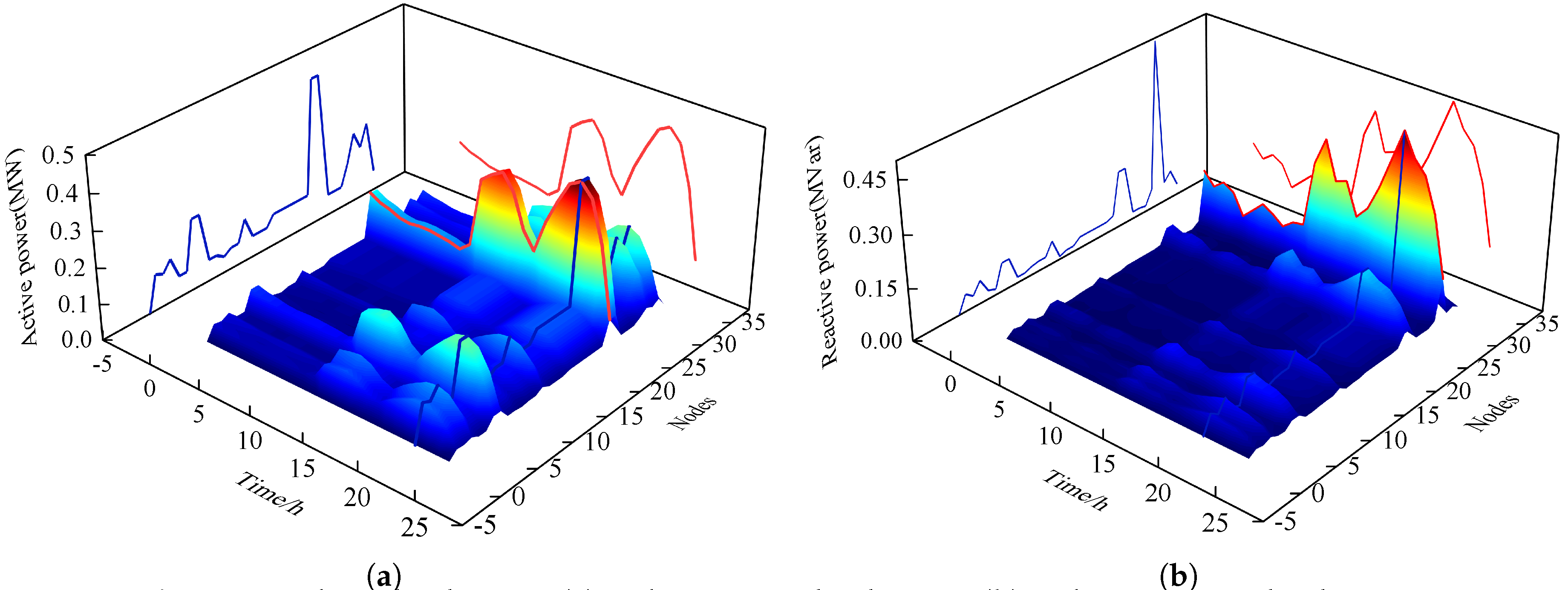
Figure 6.
PV 24-hour original active power output curve.
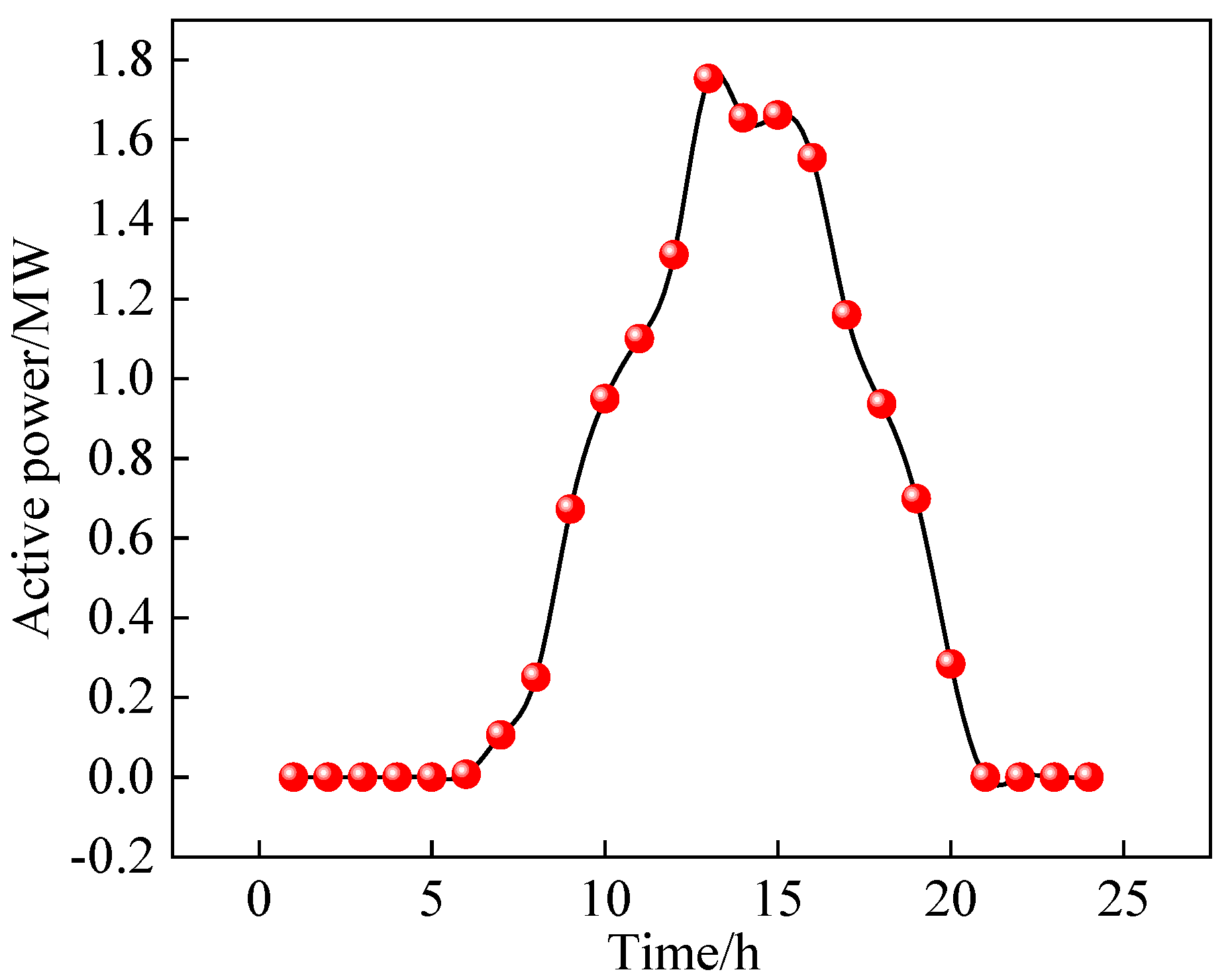
Figure 7.
24-hour OLTC dispatching strategy.
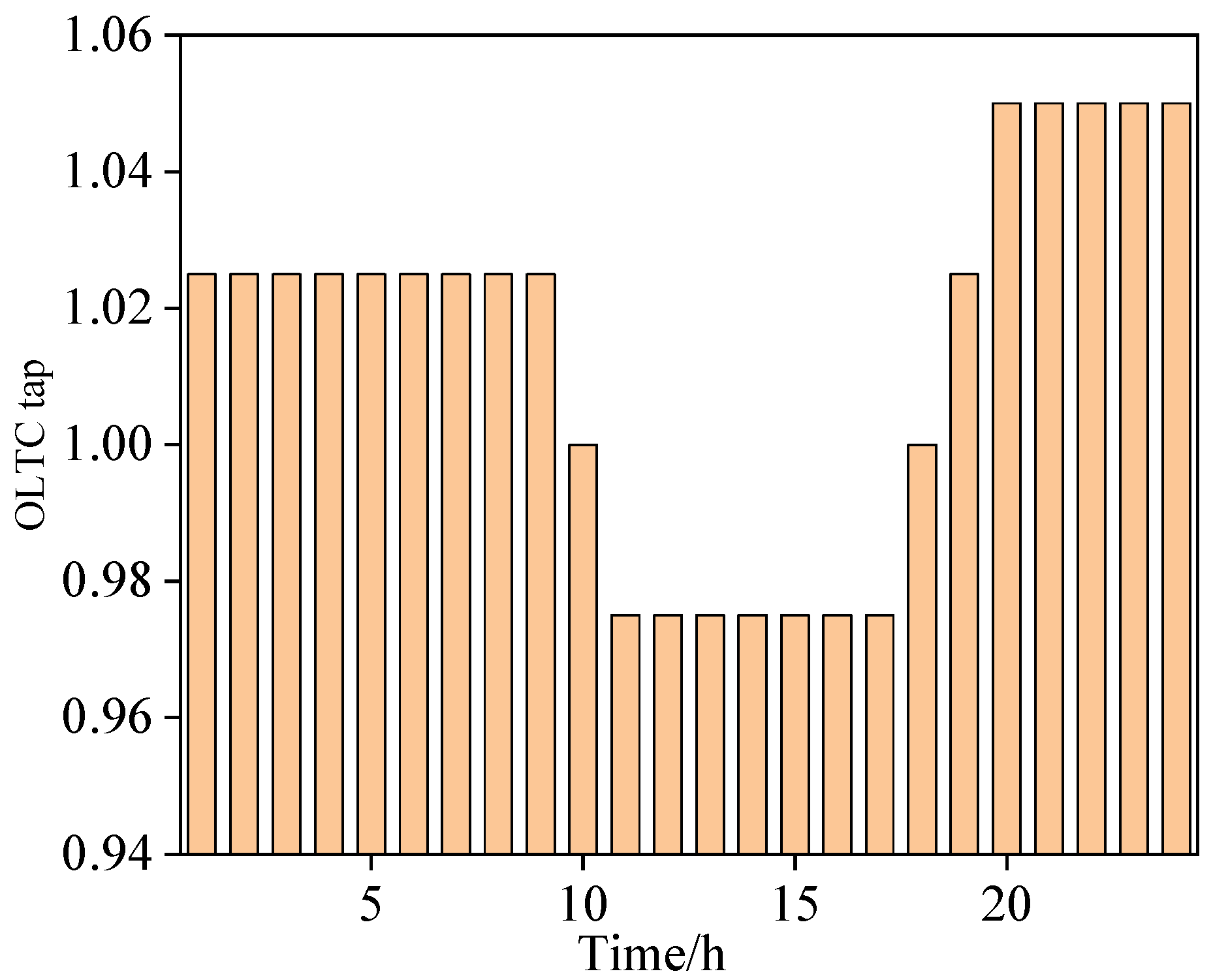
Figure 8.
24-hour CBs dispatching strategy.
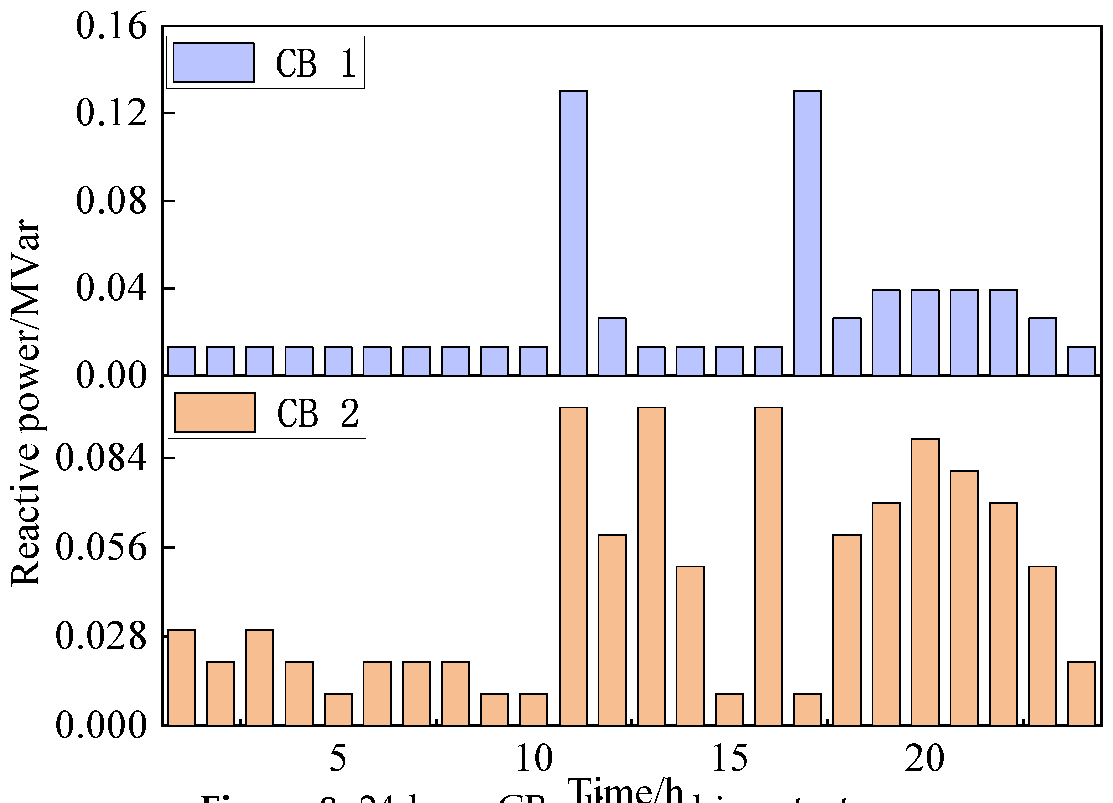
Figure 9.
Day generator active power output curve.
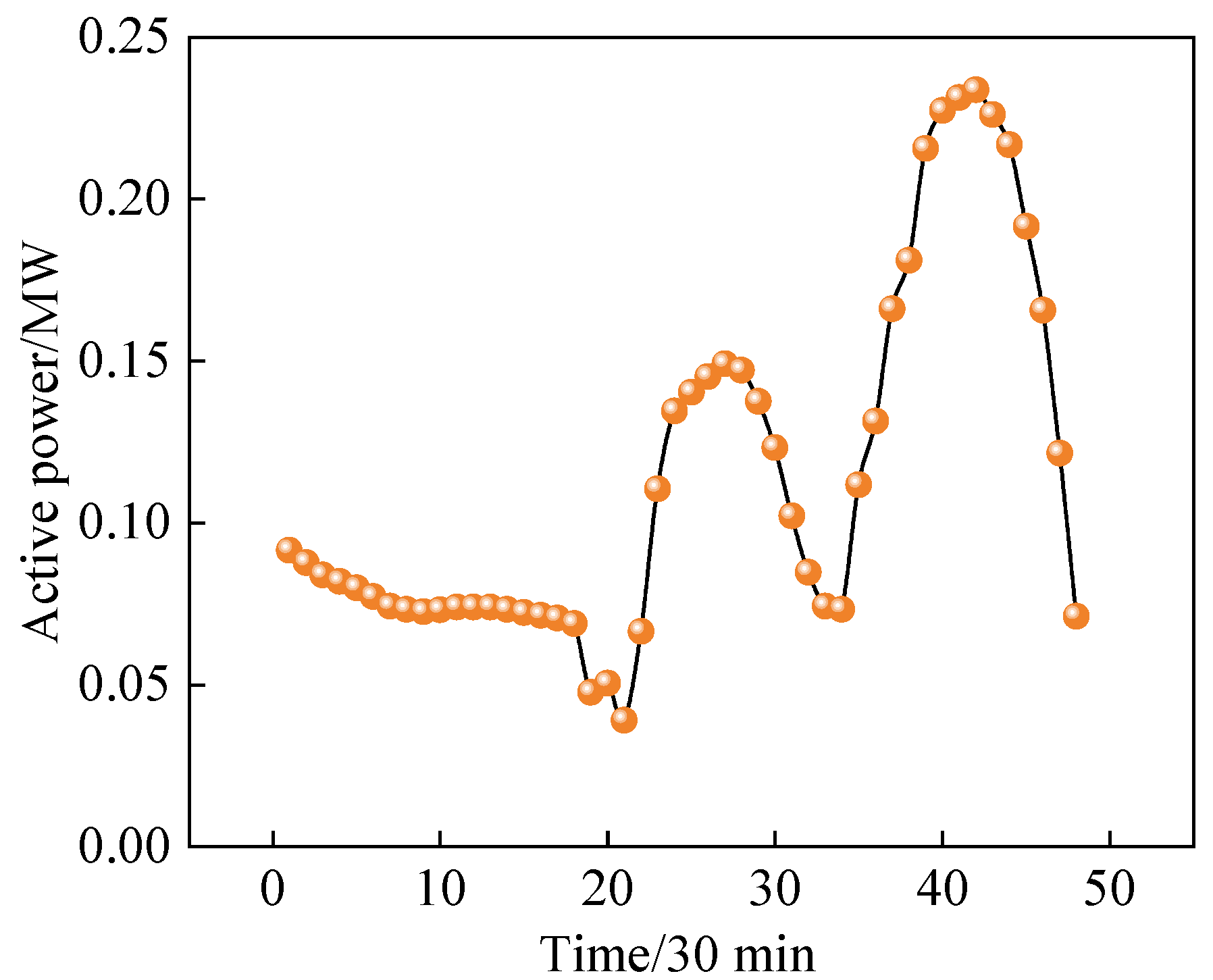
Figure 10.
Day ESs dispatching strategy.
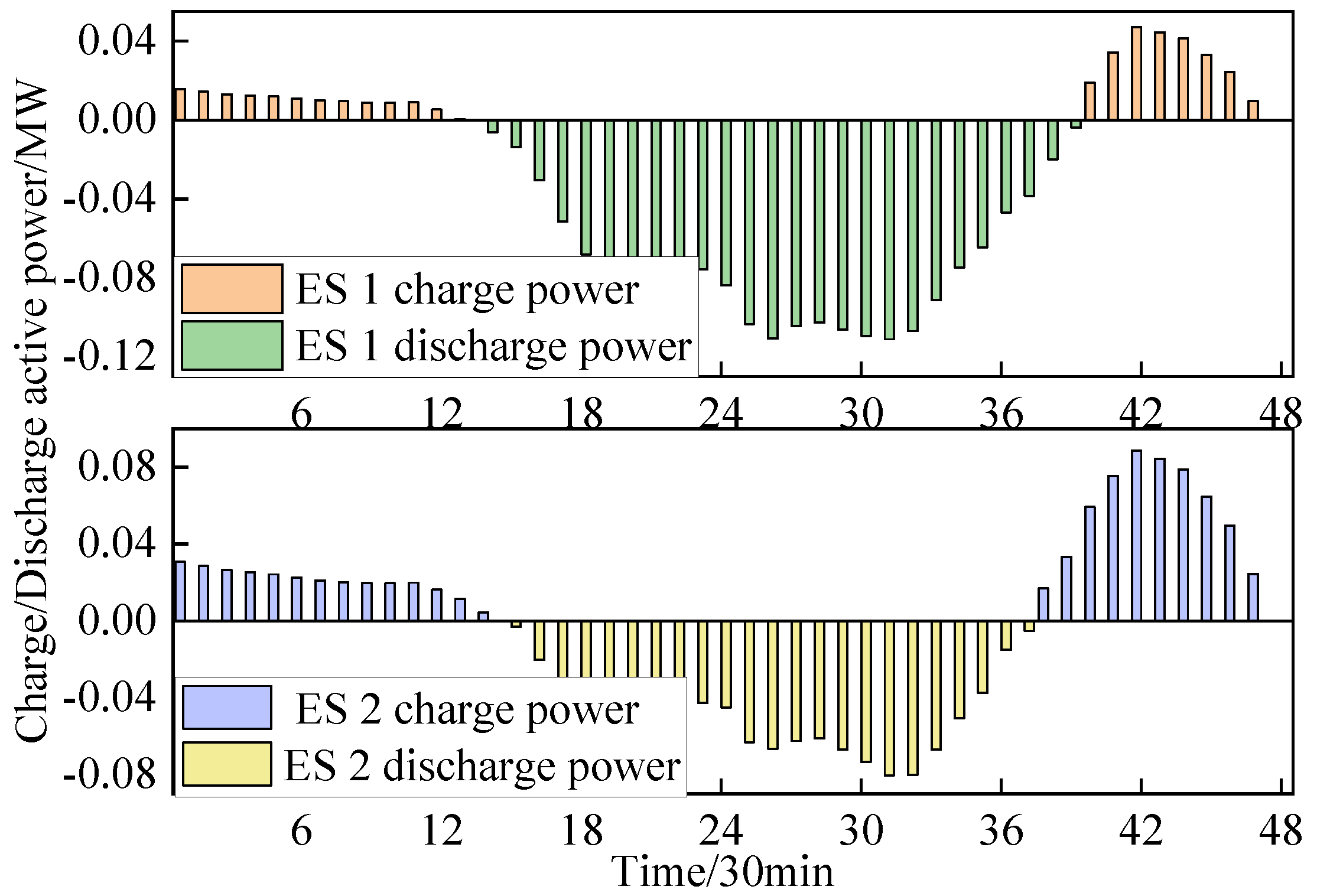
Figure 11.
Day PVs’ reactive power dispatching strategy.
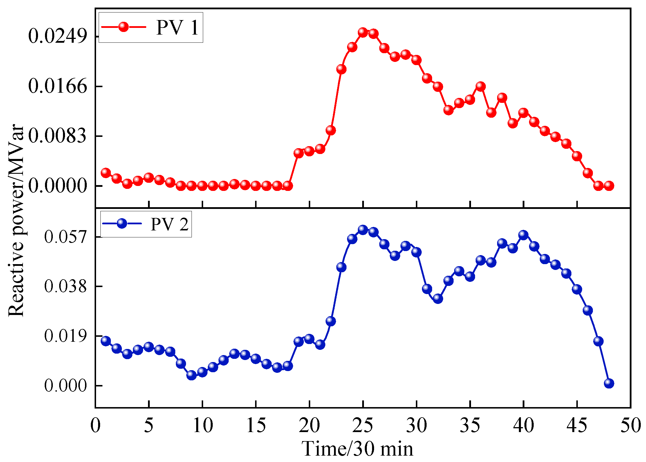
Figure 12.
Day PVs’ active power output curve before and after dispatching.
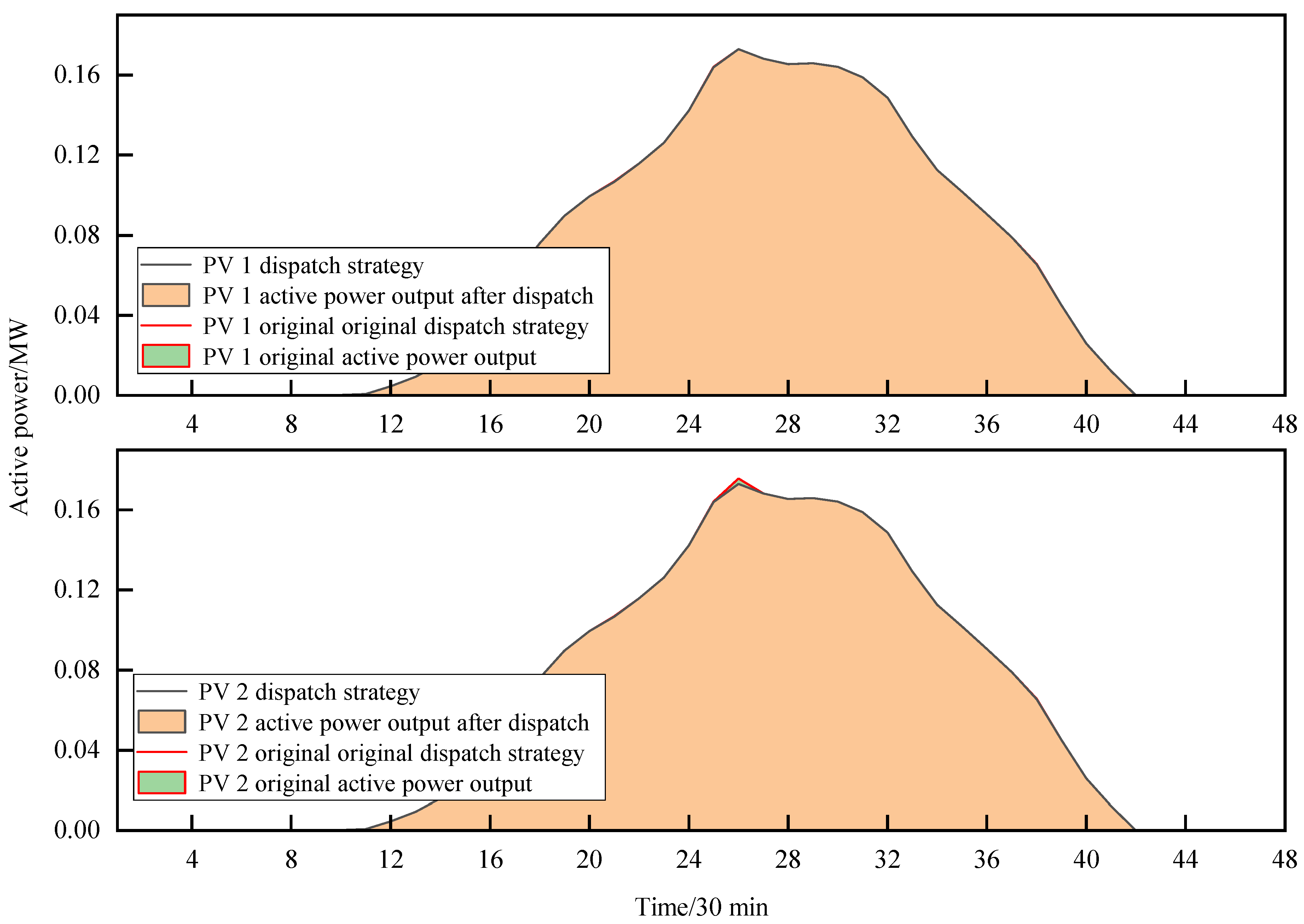
Figure 13.
ADN node voltages after optimal dispatching.
Disclaimer/Publisher’s Note: The statements, opinions and data contained in all publications are solely those of the individual author(s) and contributor(s) and not of MDPI and/or the editor(s). MDPI and/or the editor(s) disclaim responsibility for any injury to people or property resulting from any ideas, methods, instructions or products referred to in the content. |
© 2025 by the authors. Licensee MDPI, Basel, Switzerland. This article is an open access article distributed under the terms and conditions of the Creative Commons Attribution (CC BY) license (http://creativecommons.org/licenses/by/4.0/).
Copyright: This open access article is published under a Creative Commons CC BY 4.0 license, which permit the free download, distribution, and reuse, provided that the author and preprint are cited in any reuse.


