The Refined Space–Time Membrane Model: Deterministic Emergence of Quantum Fields and Gravity from Classical Elasticity

1. Introduction

Modern physics is built upon two seemingly incompatible foundations: General Relativity (GR) [1,2,3], which describes gravity through the curvature of spacetime, and Quantum Mechanics (QM) [4,5,6], whose probabilistic formalism governs microscopic phenomena. Despite remarkable successes within their respective domains, integrating these theories into a coherent framework remains one of contemporary physics’ most pressing challenges. Existing approaches—such as String Theory’s extra-dimensional constructions and Loop Quantum Gravity’s discretised spin-network formalism—provide valuable insights but have yet to deliver a definitive resolution of quantum gravity [7,8]. Meanwhile, enduring puzzles such as the black-hole information paradox and the cosmological-constant problem underline fundamental tensions between GR’s smooth geometry and QM’s intrinsic randomness [9,10,11].

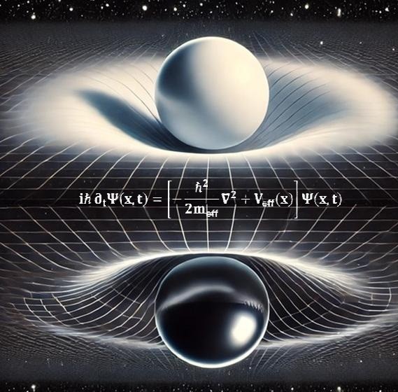
The Space–Time Membrane (STM) model proposes spacetime as a four-dimensional elastic membrane interacting with a parallel mirror domain. Every particle excitation on our “face” of the membrane has a corresponding mirror particle on the opposite face, ensuring exact matter–antimatter symmetry and addressing the observed baryon asymmetry. The membrane’s elastic dynamics simultaneously generate gravitational curvature and quantum-like phenomena: rather than postulating intrinsic randomness, apparent quantum probabilism emerges as a deterministic consequence of chaotic, sub-Planck elastic oscillations.

Concretely, the displacement field $u(x,t)$ is decomposed into two complementary oscillatory modes that combine into a two-component spinor $\mathrm{\Psi }(x,t)$. Mode-by-mode interactions between each spinor component and its mirror antispinor redistribute energy—attractive interactions generate localised curvature (gravity), while repulsive or cancelling interactions reinject energy into the membrane background. Composite photons arise as coherent wave–anti-wave cycles, in which energy exchanged in one half-cycle is precisely returned in the other, enforcing strict energy conservation even during annihilation events.

When rapid sub-Planck oscillations in u are coarse-grained, a slowly varying envelope $\psi$ emerges that obeys an effective Schrödinger-like equation. This envelope reproduces interference patterns and apparent wavefunction collapse, recasting standard quantum phenomena (including the Born rule) as manifestations of deterministic chaos. In this interpretation, Feynman’s path-integral is not an ontological sum over real histories but merely the stationary-phase approximation of a single underlying wave field; the familiar kernel

$$K(x_b,t_b;x_a,t_a)\propto \int D\left[x\left(t\right)\right]e^{{\displaystyle \frac{i}{\hslash }}S\left[x\left(t\right)\right]}$$

follows directly from a WKB/multiple-scale expansion of the STM PDE (Appendix D).

The STM framework further reinterprets key aspects of particle physics. Electroweak symmetry breaking arises from rapid zitterbewegung-like interactions between spinors and mirror antispinors, generating $W^{\pm }$ and $Z^0$ masses and yielding CP-violating phases without invoking extra scalar fields. A bimodal spinor decomposition underpins emergent gauge symmetries—U(1), SU(2) and SU(3)—as deterministic elastic connections.

The model incorporates:

• Scale-dependent elastic parameters and higher-order spatial derivatives (notably ${\nabla }^6$) to regulate ultraviolet divergences.
• Non-Markovian memory kernels to explain deterministic decoherence and effective wavefunction collapse.
• A precise bimodal decomposition of u into a two-component spinor $\mathrm{\Psi }$, yielding emergent gauge bosons.
• A deterministic electroweak symmetry-breaking mechanism via cross-membrane oscillations.
• A multi-loop renormalisation-group analysis and a nonperturbative Functional Renormalisation Group study, revealing discrete fixed points and vacuum structures that potentially account for three fermion generations.

In the gravitational sector, linearised strain fields $u_{\mu }$ link directly to metric perturbations $h_{\mu \nu }$, yielding Einstein-like field equations from the STM action—even when including damping and scale-dependent couplings (Appendix M). A detailed multi-scale derivation (Appendix H) shows that coarse-grained sub-Planck oscillations produce a near-constant vacuum offset acting as dark energy [12,13], and that a mild late-time evolution in stiffness or damping could address the Hubble tension (14).

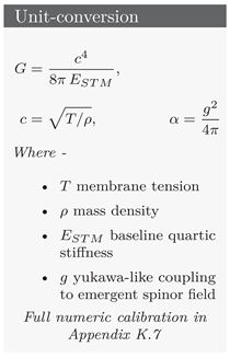
Crucially, Section 2.9—and the full parameter table in Appendix K.7—now fixes every STM coefficient to physical constants:

$$T=\rho c^2\simeq 4.82\times {10}^{42}\mathrm{Pa},E_{\mathrm{STM}}\left(\mu \right)={\displaystyle \frac{c^4}{8\pi G}},g=\sqrt{4\pi \alpha }\simeq 0.3028,$$

$${\lambda }_{\mathrm{nd}}=0.13,$$

together with the vacuum-stiffness offset $\langle \Delta E\rangle \simeq 6.8\times {10}^{-10}\mathrm{J}{\mathrm{m}}^{-3},$ a macroscopic damping coefficient ${\gamma }_{\mathrm{nd}}=0.01$ (corresponding to ${\gamma }_{\mathrm{phys}}\simeq 1.85\times {10}^{41}{\mathrm{s}}^{-1}$), and the sextic regulator ${\eta }_{\mathrm{nd}}=0.02$. These calibrations anchor the model quantitatively to the fundamental constants $c,G,\alpha$ and $\mathrm{\Lambda }$, leaving no free elastic or damping parameters.

Although STM now captures both quantum-field and cosmological-scale phenomena within one PDE, several frontiers remain.

On the thermodynamics front, we have:

• Derived the Bekenstein–Hawking entropy by micro-canonical mode counting in the STM solitonic core (Appendix F.4);
• Calculated grey-body transmission factors and effective horizon temperatures via fluctuation–dissipation (Appendix G.4–G.5);
• Sketched a Euclidean path-integral approach to the evaporation law, matching the leading-order $M^3$ timescale (Appendix H). Remaining thermodynamic tasks include subleading logarithmic and power-law corrections to the area law, Page-curve tests of unitarity and detailed first-law verifications (Appendix F.7).

Beyond thermodynamics, our analytic derivations (Appendices C and N) detail mode-by-mode spinor–antispinor couplings, while recent numerics anchored to physically motivated parameters reveal three well-separated mass minima that reproduce the Standard Model’s generational hierarchy, mixing angles and CP-violating phases (Section 3.1.4 & 4.3). Early tests (Section 3.3; Appendix K.7) suggested the damping coefficient $\gamma$ might be dispensable, but a full analysis of measurement dynamics and deterministic wavefunction collapse (Section 3.4) confirms that a finite $\gamma$ is essential. Although $\gamma$ introduces mild non-conservatism, the model remains stable across a broad range of values.

Appendix T now proves global well-posedness, self-adjointness and ghost-freedom on any globally-hyperbolic manifold (Theorem T.1; Proposition T.2), while Appendix U shows that gauge, mixed and gravitational anomalies cancel identically via mirror doubling. With these foundational issues resolved, future work narrows to a spin–statistics theorem for the bimodal spinors, higher-loop renormalisation and the microstate structure of black holes. Addressing the remaining challenges will be crucial to establishing the STM framework’s consistency across all scales.

Unlike many quantum-gravity schemes, the STM model is rooted in classical continuum elasticity, so it can be tested directly through numerical simulations and laboratory analogues such as metamaterials. By deriving Schrödinger dynamics, the Born rule, gauge symmetries and CP violation from a single deterministic PDE, STM uses far fewer independent postulates than frameworks of comparable scope—for example, the Standard Model plus general relativity, which require separate fundamental fields and symmetry assumptions. Approaches with an even sparser axiomatic core (e.g. asymptotically safe gravity) typically focus on the gravitational sector alone and do not yet reproduce the full gauge and flavour structure that STM aims to encompass.

We therefore encourage further numerical, experimental and theoretical exploration of the STM model as a promising, conceptually transparent route to reconciling quantum phenomena with gravitational curvature.

Organisation of the Paper

• Section 2 (Methods) provides a detailed overview of the STM wave equation, including explicit derivations of higher-order elasticity terms, spinor construction, scale-dependent parameters, and the deterministic interpretation of decoherence.
• Section 3 (Results) demonstrates how quantum-like dynamics, the Born rule, entanglement analogues, emergent gauge fields ($U\left(1\right)$, $SU\left(2\right)$, $SU\left(3\right)$), deterministic decoherence, fermion generations, and CP violation naturally arise from the deterministic membrane equations.
• Section 4 (Discussion) explores the broader implications of these findings, along with possible experimental tests and numerical simulations.
• Section 5 (Conclusion) summarises the key theoretical advances, outstanding issues, and potential future directions, including proposals aimed at verifying the STM model’s predictions.

Appendices A–U comprehensively present supporting details, derivations, and numerical methods. They address:

• Operator Formalism and Spinor Field Construction (Appendix A)
• Derivation of the STM Elastic-Wave Equation and External Force (Appendix B)
• Gauge symmetry emergence and CP violation (Appendix C)
• Coarse-grained Schrödinger-like dynamics (Appendix D)
• Deterministic entanglement (Appendix E)
• Singularity avoidance (Appendix F)
• Non-Markovian Decoherence and Measurement (Appendix G)
• Vacuum energy dynamics and the cosmological constant (Appendix H)
• Proposed experimental tests (Appendix I)
• Renormalisation Group Analysis and Scale-Dependent Couplings (Appendix J)
• Finite-Element Calibration of STM Coupling Constants (Appendix K)
• Nonperturbative analyses revealing solitonic structures (Appendix L)
• Covariant Generalisation and Derivation of Einstein Field Equations (Appendix M)
• Emergent Scalar Degree of Freedom from Spinor–Mirror Spinor Interactions (Appendix N)
• Rigorous Operator Quantisation and Spin-Statistics (Appendix O)
• Reconciling Damping, Environmental Couplings, and Quantum Consistency in the STM Framework (Appendix P)
• Toy Model PDE Simulations (Appendix Q)
• First principles derivations of CKM and PMNS matrices (Appendix R)
• STM Scattering Amplitude Validation (Appendix S)
• Well-Posedness and Ghost-Freedom of the STM PDE (Appendix T)
• Anomaly Cancellation in the STM Model (Appendix U)

Finally, an updated Appendix V serves as a Glossary of Symbols, ensuring clarity and consistency of notation throughout.

2. Methods

In the Space–Time Membrane (STM) model, spacetime is represented as a four-dimensional elastic membrane governed by a deterministic high-order partial differential equation. This single PDE unifies gravitational-scale curvature with quantum-like oscillations by incorporating higher-order elasticity, scale-dependent stiffness, non-linear terms, and possible non-Markovian effects. Below, we provide the theoretical foundations, outline the operator quantisation that yields quantum-like behaviour, show how gauge fields naturally emerge, discuss renormalisation strategies, and comment on the classical limit.

2.1. Classical Framework and Lagrangian

2.1.1. Displacement Field and Equation of Motion

We begin with a real displacement field $u(x,t)$, which tracks local deformations of a classical four-dimensional membrane (see Section 1.2). The STM model augments standard elasticity with membrane tension, higher-order spatial derivatives and scale-dependent parameters, leading to the PDE

$$\rho {\displaystyle \frac{{\partial }^{2}u}{\partial t^2}}+T{\nabla }^{2}u-\left[E_{STM}\left(\mu \right)+\Delta E(x,t;\mu )\right]{\nabla }^{4}u+\eta {\nabla }^{6}u-\gamma {\displaystyle \frac{\partial u}{\partial t}}-\lambda u^3-gu\overline{\mathrm{\Psi }}\mathrm{\Psi }+F_{ext}(x,t)=0.$$

(A full variational derivation is given in Appendix B)

Note: Every spatial derivative already carries the implicit factor $l_P^{-1}$ used in Appendices K.6–K.7; no explicit $l_P^{-2n}$ denominators are required. Hence each term in (2.1) has units of pressure (Pa), matching the calibrated SI values in Appendix K.7.

Key ingredients:

• $\rho$: effective mass density describing inertial response
• T: membrane tension, stiffening long-wavelength modes
• $E_{STM}\left(\mu \right)$: baseline elastic modulus at renormalisation scale $\mu$
• $\Delta E(x,t;\mu )$: local stiffness variations; its uniform part acts like vacuum energy once fast oscillations are averaged out
• $\eta {\nabla }^{6}u$: sixth-order regularisation damping ultraviolet modes
• $\gamma {\partial }_{t}u$: viscous damping, extensible to non-Markovian kernels
• $\lambda u^3$: non-linear self-interaction
• $-gu\overline{\mathrm{\Psi }}\mathrm{\Psi }$: Yukawa-like coupling to an emergent spinor field $\mathrm{\Psi }$
• $F_{ext}(x,t)$: external forcing or boundary effects.

While not appearing in the scalar PDE,the term ${\gamma }_f$ spinor dephasing - represents a milder damping (${\gamma }_f={\displaystyle \frac{1}{2}}\gamma$) that appears in the Dirac-like equations for the spinor and mirror-spinor fields, ensuring flavour decoherence occurs on the same physical timescale as scalar Born-rule collapse. ${\gamma }_f$ is not an independent constant; coarse-graining fixes it to ${\gamma }_f={\displaystyle \frac{1}{2}}\gamma$ (see Section 3.4.1 and Appendix K.6).

This PDE provides a unified mathematical context in which large-scale curvature emerges as low-frequency deformations and short-scale oscillations mimic quantum phenomena—without extra dimensions or intrinsic randomness.

2.1.2. Lagrangian Density

Omitting damping and forcing for clarity, the Euler–Lagrange equation of Section 2.1.1 follows from the Lagrangian density

$$L={\displaystyle \frac{1}{2}}\rho {\left({\partial }_{t}u\right)}^2-{\displaystyle \frac{1}{2}}T{(\nabla u)}^2-{\displaystyle \frac{1}{2}}[E_{STM}\left(\mu \right)+\Delta E(x,t;\mu )]{\left({\nabla }^{2}u\right)}^2-{\displaystyle \frac{1}{2}}\eta {\left({\nabla }^{3}u\right)}^2-V\left(u\right),$$

where $V\left(u\right)$ captures any polynomial or non-polynomial self-interactions (e.g.\ ${\displaystyle \frac{1}{2}}k{u}^2$, ${\displaystyle \frac{1}{4}}\lambda u^4$, etc.). Integrating over space–time gives $S=\int L{d}^{4}x$, and imposing $\delta S=0$ under suitable boundary conditions recovers the full PDE. Effective dissipation functionals may be appended to include $\gamma {\partial }_{t}u$ or non-Markovian memory kernels (Appendix B).

2.1.3. Hamiltonian Formulation and Poisson Brackets

Starting from the Lagrangian density of §2.1.2,

$$L={\displaystyle \frac{1}{2}}\rho {\left({\partial }_{t}u\right)}^2-{\displaystyle \frac{1}{2}}T{(\nabla u)}^2-{\displaystyle \frac{1}{2}}[E_{STM}\left(\mu \right)+\Delta E(x,t;\mu )]{\left({\nabla }^{2}u\right)}^2-{\displaystyle \frac{1}{2}}\eta {\left({\nabla }^{3}u\right)}^2-V\left(u\right),$$

we proceed as follows:

Conjugate momentum

$$\pi (\mathbf{x},t)={\displaystyle \frac{\partial L}{\partial \left({\partial }_{t}u\right)}}=\rho {\partial }_{t}u(\mathbf{x},t).$$

Legendre transform

The Hamiltonian density is

$$\mathcal{H}=\pi {\partial }_{t}u-L={\displaystyle \frac{1}{2}}\rho {\left({\partial }_{t}u\right)}^2+{\displaystyle \frac{1}{2}}T{(\nabla u)}^2+{\displaystyle \frac{1}{2}}(E_{STM}+\Delta E){\left({\nabla }^{2}u\right)}^2$$

$$+{\displaystyle \frac{1}{2}}\eta {\left({\nabla }^{3}u\right)}^2+V\left(u\right).$$

Canonical structure and Dirac rule

The fundamental Poisson bracket is

$${\{u\left(x\right),\pi \left(y\right)\}}_{PB}={\delta }^3(x-y)\left(\mathrm{see}\mathrm{Appendix}\mathrm{C}\right).$$

• Demanding that this symplectic structure survive coarse-graining enforces the Dirac rule

$${\{·,·\}}_{\mathrm{PB}}⟶{\displaystyle \frac{1}{i\hslash }}[·,·],$$

• from which the operator commutator

$$[\widehat{u}\left(x\right),\widehat{\pi }\left(y\right)]=i\hslash {\delta }^3(x-y)$$

• follows directly from the membrane’s elasticity, rather than being imposed by hand.

Quantum Hamiltonian

Promoting fields to operators and integrating over space,

$$-{\displaystyle \frac{T}{2}}\int \mid \nabla \widehat{u}{\mid }^2{d}^{3}x$$

• Note: the ${\displaystyle \frac{T}{2}}{(\nabla \widehat{u})}^2$ term contributes $-{\displaystyle \frac{T}{2}}\int {|\nabla \widehat{u}|}^2{d}^{3}x$ with no operator-ordering ambiguity (Appendix C).

While initial numerical investigations in Section 3.3 identified stable parameter regimes without explicit damping, a detailed analysis of deterministic measurement processes and the Born rule (Section 3.4) conclusively demonstrates that a small positive damping term is necessary to ensure physical consistency and correct quantum predictions.

A rigorous curved-spacetime proof that this Hamiltonian remains self-adjoint, ghost-free and globally well-posed is now given in Appendix T (Theorem T.1 and Proposition T.2).

2.1.4. Conjugate Momentum and Modified Dispersion

From the Lagrangian density, the conjugate momentum to u is defined by

$$\pi (\mathbf{x},t)={\displaystyle \frac{\partial L}{\partial \left({\partial }_{t}u\right)}}=\rho {\partial }_{t}u(\mathbf{x},t).$$

Assuming plane-wave solutions in a homogeneous setting (cf. §3.2), take the ansatz

$$u(\mathbf{x},t)=u_0{e}^{i(k·x-\omega t)}.$$

Substituting into the linearised PDE of Section 2.1.1, use

$${\partial }_t^{2}u\to -{\omega }^{2}u,{\nabla }^{2}u\to -{\left|k\right|}^{2}u,{\nabla }^{4}u\to {\left|k\right|}^{4}u,{\nabla }^{6}u\to -{\left|k\right|}^{6}u,$$

which yields the algebraic relation

$$-\rho {\omega }^2+T\mid k{\mid }^2+(E_{STM}+\Delta E)\mid k{\mid }^4+\eta \mid k{\mid }^6=0.$$

Solving for ${\omega }^2$ gives

$${\omega }^2\left(k\right)={\displaystyle \frac{T}{\rho }}\mid k{\mid }^2+{\displaystyle \frac{E_{STM}+\Delta E}{\rho }}\mid k{\mid }^4+{\displaystyle \frac{\eta }{\rho }}\mid k{\mid }^6.$$

• Long-wavelength limit ($\left|k\right|\to 0$): tension-dominated ${(T/\rho )\left|k\right|}^2$.
• Intermediate regime: bending rigidity $(E+\Delta E)/{\rho \left|k\right|}^4$.
• Ultraviolet regularisation ($\left|k\right|\to \infty$): sixth-order term ${(\eta /\rho )\left|k\right|}^6$.

When $\Delta E(x,t;\mu )$ is significant, one replaces a simple plane-wave approach with advanced numerical methods (see Section 2.4 and Appendix K) or a Bloch-like analysis if $\Delta E$ is spatially periodic.

2.2. Operator Quantisation

2.2.1. Canonical Commutation Relations

Building on the Hamiltonian structure just introduced, we promote the displacement field $u(x,t)$ and its conjugate momentum $\pi (x,t)$ a to operators $\widehat{u}(x,t)$ and $\widehat{\pi }(x,t)$ on a suitable Sobolev domain. The classical Poisson bracket

$${\{u\left(x\right),\pi \left(y\right)\}}_{PB}={\delta }^3(x-y)$$

is elevated via the Dirac correspondence

$${\{·,·\}}_{PB}⟶{\displaystyle \frac{1}{i\hslash }}[·,·],$$

which immediately yields

$$[\widehat{u}(x,t),\widehat{\pi }(y,t)]=i\hslash {\delta }^3(x-y),$$

with all other commutators vanishing. Thus the non-commutativity of $\widehat{u}$ and $\widehat{\pi }$ emerges naturally from the membrane’s intrinsic symplectic form, without requiring an extra quantisation postulate.

2.2.2. Normal Mode Expansion

In nearly uniform regions, one may write

$$\widehat{u}(x,t)=\int {\displaystyle \frac{d^{3}k}{{\left(2\pi \right)}^3}}{e}^{ik·x}\widehat{u}(k,t),\widehat{\pi }(k,t)\mathrm{similarly}.$$

The associated Hamiltonian sums over the modes, each with a modified dispersion $\omega \left(k\right)$. When $\Delta E$ varies, a real-space diagonalisation or finite element approach is more suitable. Either way, the operator quantisation ensures a “quantum-like” spectrum of excitations that parallels bosonic fields in standard quantum theory.

2.3. Gauge Symmetries: Emergent Spinors and Path Integral

2.3.1. Bimodal Decomposition and Emergent Gauge Fields

A distinctive aspect of the STM model is constructing a bimodal decomposition of $\widehat{u}(x,t)$. Formally, one splits u into two complementary oscillatory components, sometimes referred to as in-phase and out-of-phase fields:

$$u_1(x,t)={\displaystyle \frac{u+u_{\perp }}{\sqrt{2}}},u_2(x,t)={\displaystyle \frac{u-u_{\perp }}{\sqrt{2}}},$$

and arranges $\left(u_1,u_2\right)$ into a two-component spinor $\mathrm{\Psi }(x,t)$. Imposing a local phase invariance $\mathrm{\Psi }\to e^{i\alpha (x,t)}\mathrm{\Psi }$ necessitates the introduction of gauge fields, e.g.\ $A_{\mu }$ for $U\left(1\right)$. Extending this principle can yield non-Abelian fields $W_{\mu }^a$$\left(SU\left(2\right)\right)$ and $G_{\mu }^a$ $\left(SU\left(3\right)\right)$, reproducing the main gauge bosons familiar from the electroweak and strong interactions [15,16].

Mechanically, each gauge field arises as a compensating “connection” ensuring that local redefinitions of the spinor field do not alter physical observables. Consequently, photon-like or gluon-like excitations appear as coherent wave modes in the membrane. In standard quantum field theory, “virtual particles” mediate interactions; here, such processes correspond to deterministic wave–anti-wave cycles wherein net energy transfer over a full cycle is zero, aligning with the virtual-exchange picture. By including local phase invariance in the STM action, one automatically generates covariant derivatives $D_{\mu }={\partial }_{\mu }-ig{A}_{\mu }$ (or the non-Abelian analogue), reinforcing how gauge fields naturally emerge from the underlying elasticity.

In the path-integral language, enforcing local spinor symmetries introduces these gauge connections and ghost fields (for gauge fixing) but does not rely on intrinsic randomness. Instead, it unites the deterministic elasticity framework with internal gauge invariance. This places photon-like excitations (for U(1)), $W^{\pm }$ bosons (for SU(2)), and gluons (for SU(3)) as collective membrane oscillations that preserve local symmetry at each point in spacetime.

2.3.2. Ontology of Non-Abelian Gauge Fields

In STM the familiar non-Abelian gauge symmetries SU(2) and SU(3) arise in exactly the same way as U(1), only now acting on higher-dimensional internal oscillator spaces. Concretely:

SU(2) as Local Doublet Rotations

At each spacetime point the STM spinor is promoted to a two-component doublet $\mathrm{\Psi }=({\mathrm{\Psi }}_1,{\mathrm{\Psi }}_2)$. The internal freedom to rotate

$$\mathrm{\Psi }\left(x\right)\mapsto U\left(x\right)\mathrm{\Psi }\left(x\right),U\left(x\right)\in SU\left(2\right),$$

corresponds to choosing a new basis in the two-mode oscillator plane.

To compare $\mathrm{\Psi }\left(x\right)$ and $\mathrm{\Psi }(x+dx)$ without ambiguity we introduce the matrix-valued connection $A_{\mu }\left(x\right)\in \mathfrak{su}\left(2\right)$, so that the covariant derivative $D_{\mu }\mathrm{\Psi }={\partial }_{\mu }\mathrm{\Psi }-ig{A}_{\mu }\mathrm{\Psi }$ remains well-defined under local SU(2) rotations.

Physically, each generator of SU(2) is realised as a distinct “twist” or shear of the STM membrane’s two-mode oscillation, and the Yang–Mills field strength $F_{\mu \nu }={\partial }_{\mu }{A}_{\nu }-{\partial }_{\nu }{A}_{\mu }-i[A_{\mu },A_{\nu }]$ measures the membrane’s curvature in that internal rotation space.

SU(3) as Local Triplet Rotations

Similarly, for colour we carry a three-component oscillator $\mathrm{\Psi }=({\mathrm{\Psi }}_1,{\mathrm{\Psi }}_2,{\mathrm{\Psi }}_3)$ transforming under local SU(3) rotations $\mathrm{\Psi }\mapsto U\left(x\right)\mathrm{\Psi },U\in SU\left(3\right)$.

An eight-component connection $A_{\mu }^a{T}^a$ (with $T^a$ the Gell-Mann generators) compensates infinitesimal changes in that three-mode orientation, yielding $D_{\mu }\mathrm{\Psi }={\partial }_{\mu }\mathrm{\Psi }-i{g}_s{A}_{\mu }^a{T}^a\mathrm{\Psi }$.

The associated field strength $F_{\mu \nu }^a={\partial }_{\mu }{A}_{\nu }^a-{\partial }_{\nu }{A}_{\mu }^a+g_s{f}^{abc}{A}_{\mu }^b{A}_{\nu }^c$ is nothing but the elastic-energy cost of non-commuting shears in the membrane’s colour-triplet oscillation bundle.

Unified Membrane Interpretation

In every case, gauge symmetry is simply the freedom to rotate the internal oscillator basis at each point in a way that costs elastic energy when misaligned.

All familiar Maxwell or Yang–Mills Lagrangians arise from writing down the membrane’s elastic energy as the square of these curvature two-forms.

Thus, U(1), SU(2) and SU(3) gauge fields share a single ontological origin: the tangent-space rotations of the STM membrane’s multimode oscillations.

No mandatory high-energy convergence

Because U(1), SU(2) and SU(3) all arise as different rotational polarisations of the same four-dimensional membrane, their common origin is already encoded in the Lagrangian. The usual grand-unification requirement $g_1=g_2=g_3$ at some ultra-high scale is therefore optional, not obligatory. Functional-RG trajectories in Appendix J show that for some stiffness ratios the three couplings can approach one another near the sextic fixed point, but nothing in the STM dynamics enforces that coincidence. Hence proton-decay bounds do not constrain STM, and the model accommodates either convergent or non-convergent running without additional fields.

2.3.3. Virtual Bosons as Deterministic Oscillations

In standard quantum field theory, “virtual particles” are ephemeral excitations in Feynman diagrams [17]. Here, such processes are reinterpreted as perfectly energy-balanced wave–plus–anti-wave cycles. Over one cycle, net energy transfer is zero, consistent with the notion of a virtual exchange. Hence, interactions that appear “probabilistic” from a standard QFT perspective gain a deterministic wave interpretation in the STM model.

In path-integral language [18], the partition function

$$Z=\int DuD{A}_{\mu }D\left(\mathrm{ghosts}\right)exp\left\{i{S}_{STM}[u,A_{\mu }]\right\}$$

incorporates both the displacement field u (with higher-order derivatives) and the gauge fields that emerge upon enforcing local spinor-phase invariance. Ghost fields appear as usual for gauge fixing and do not introduce fundamental randomness—they merely handle redundant field configurations in a deterministic continuum.

2.4. Renormalisation and Higher-Order Corrections

2.4.1. One-Loop and Multi-Loop Analyses

The sixth-order operator $\eta {\nabla }^{6}u$ ensures strong damping of high-momentum modes, so loop integrals converge more rapidly than in a naive second-order theory. Standard dimensional regularisation and a BPHZ subtraction scheme can be applied to compute self-energy corrections at one-loop or higher orders (see Appendix J). The resulting beta functions typically take the schematic form:

$$\beta \left(g_{eff}\right)=a{g}_{eff}^2+b{g}_{eff}^3+\dots ,$$

where $a,b$ are integrals influenced by $\mid k{\mid }^4$ and $\mid k{\mid }^6$ factors in the propagator. Multi-loop diagrams, including “setting sun” or mixed fermion–scalar topologies, refine these flows further. Crucially, running elastic couplings $E_{STM}\left(\mu \right)$ and $\Delta E(x,t;\mu )$ can exhibit non-trivial fixed points, opening the door to multiple stable vacua or discrete mass spectra.

2.4.2. Nonperturbative FRG and Solitons

Perturbation theory alone cannot capture phenomena like solitonic black hole cores or multiple vacuum states. Thus, a Functional Renormalisation Group (FRG) approach (see Appendix L) is employed, tracking an effective action ${\mathrm{\Gamma }}_k\left[u\right]$ as fluctuations are integrated out down to scale k. This approach can reveal topologically stable solutions (e.g.\ kinks, domain walls) crucial for:

• Fermion generation: Multiple minima in the effective potential can produce distinct mass scales, paralleling three observed fermion generations.
• Black hole regularisation: Enhanced stiffness from $\Delta E$ and ${\nabla }^6$ stops curvature blow-up, replacing singularities with finite-amplitude standing waves.

2.5. Classical Limit and Stationary-Phase Approximation

In a classical or macroscopic regime, one sets $\hslash \to 0$ or assumes heavy damping. The path integral

$$\int Duexp\left\{{\displaystyle \frac{i}{\hslash }}{S}_{STM}\left[u\right]\right\}$$

is dominated by stationary-phase solutions of the PDE. Thus, the membrane behaves as a purely classical object with fourth- and sixth-order elasticity. Conversely, at sub-Planck scales—where the chaotic interplay of $\Delta E$ and ${\nabla }^6$ acts—coarse-graining these rapid oscillations yields interference, Born-rule-like probability patterns, and gauge bosons as emergent wave modes (Appendix D).

Thus the familiar Schrödinger equation and its path-integral form are simply calculational devices—valid envelope approximations to our single, deterministic STM wave equation—rather than fundamental postulates of nature.

2.6. Non-Markovian Decoherence and Wavefunction Collapse

While the PDE is entirely deterministic, real-world observations show effective wavefunction collapse. In the STM model, this arises from non-Markovian decoherence: one splits u into slow (system) and fast (environment) parts, integrates out the environment in a Feynman–Vernon influence functional, and obtains a memory-kernel master equation for the reduced density matrix of the slow component [19]. Off-diagonal elements of this density matrix decay deterministically due to finite correlation times, reproducing an apparent measurement collapse. Thus, wavefunction reduction becomes an emergent, history-dependent phenomenon, rather than a postulate of fundamental randomness.

Such non-Markovian behaviour also underlies deterministic entanglement analogues (Appendix E), showing how Bell-inequality violations appear in a classical continuum. The rate and mechanism of decoherence can, in principle, be studied in laboratory analogues and metamaterial experiments (Section 4.1, Appendix I).

2.7. Persistent Waves, Dark Energy, and the Cosmological Constant

In the long-wavelength, low-frequency limit $(k\ll k_{*})$ the full STM elasticity equation of Appendix B

$$\rho {\partial }_t^{2}u+T{\nabla }^{2}u-[E_{STM}+\Delta E(x,t)]{\nabla }^{4}u+\eta {\nabla }^{6}u=0$$

reduces (because the ${\nabla }^4$ and ${\nabla }^6$ operators are suppressed by $k^2$ and $k^4$). The surviving terms may be written

$$\begin{array}{c}\square u+{\displaystyle \frac{T}{\rho }}u+\langle \Delta E\rangle \left(t\right)u=0\\ \square ={\rho }^{-1}\left({\partial }_t^2-c^2{\nabla }^2\right),c^2={\displaystyle \frac{T}{\rho }}\end{array}$$

with

$$\langle \Delta E\rangle \left(t\right)={\displaystyle \frac{1}{V}}\int \Delta E(x,t)d^{3}x$$

Here and throughout, every spatial derivative carries an implicit factor $L_P$ and $\rho \equiv {\rho }_P{L}_P^{-2}$, so each term in the equation has the common units of pressure $J{m}^{-3}=Pa$ .

$\langle \Delta E\rangle$ is the spatially uniform component of the scale-dependent modulus discussed in Appendix H.4.

A “Eureka” reinterpretation of the double-slit

Eureka moment. Treating the double-slit fringes as elastic standing waves immediately reveals a puzzle: such waves cannot persist unless the membrane receives a continuous energy trickle. STM resolves this by recognising that rapid mirror exchange (Appendix P) modulates the local modulus, producing the slow feedback $\langle \Delta E\rangle \left(t\right)$ that phase-locks the oscillations. The very same mechanism that keeps laboratory interference alive therefore seeds a tiny, uniform stiffness offset on cosmological scales.

B Emergent cosmological constant

The strain-to-curvature map of Appendix M.6 identifies the constant offset with a vacuum-energy term

$$\mathrm{\Lambda }={\displaystyle \frac{8\pi G}{c^4}}\langle \Delta E\rangle .$$

Because $E_{STM}\simeq c^4/8\pi G\approx 4.82\times {10}^{42}\mathrm{Pa}$, an imperceptible fractional shift

$${\displaystyle \frac{\langle \Delta E\rangle }{E_{STM}}}\sim {10}^{-53}$$

reproduces the observed dark-energy density ${\rho }_{\mathrm{\Lambda }}\approx {10}^{-9}\mathrm{Pa}$. Thus STM links quantum interference and cosmic acceleration without introducing extra fields or stochastic postulates.

C Ultraviolet safety and solitonic cores

At large strain the sextic regulator $\eta {\nabla }^{6}u$ dominates, raising the effective stiffness and preventing divergences. Appendix M.7 shows this caps curvature inside collapsing regions, replacing general-relativistic singularities with finite-energy solitonic cores that still satisfy $S_{BH}=A/4G\hslash$.

D Numerical window

Even with $\langle \Delta E\rangle /E_{STM}\sim {10}^{-53}$, quartic and sextic terms re-enter at LIGO-band strains ($\sim {10}^{31}\mathrm{Pa}$), far above laboratory scales yet well below the Planck modulus—ensuring consistency from tabletop interferometers to gravitational-wave astronomy.

In essence, a single eight-parameter elasticity law explains persistent quantum fringes, an effective cosmological constant and singularity avoidance. The “eureka” insight—that double-slit coherence demands an elastic feedback term—turns out to be the same ingredient that could drive the Universe’s late-time acceleration.

2.8. Action Principle in Curved Spacetime

2.8.1. Action Principle

We embed the STM framework on a four-dimensional Lorentzian manifold $(M,g_{\mu \nu })$ by introducing a single action

$$S={\int }_M{d}^{4}x\sqrt{-g}[{\displaystyle \frac{c^4}{16\pi G}}R+{\mathcal{L}}_{\varphi }+{\mathcal{L}}_{\mathrm{\Psi }}+{\mathcal{L}}_{int}],$$

where R is the Ricci scalar of the metric $g_{\mu \nu }$. The STM Lagrangian splits into three parts:

• the scalar “membrane” sector ${\mathcal{L}}_{\varphi }$,
• the two-component spinor sector ${\mathcal{L}}_{\mathrm{\Psi }}$, and
• their elastic interaction ${\mathcal{L}}_{int}$.

All ordinary derivatives are replaced by Levi–Civita covariant derivatives, and each elastic constant enters as a diffeomorphism-invariant scalar. In particular, we define

$$\square :={\nabla }^{\mu }{\nabla }_{\mu },\{{\gamma }^{\mu },{\gamma }^{\nu }\}=2g^{\mu \nu },\overline{\mathrm{\Psi }}={\mathrm{\Psi }}^{†}{\gamma }^0.$$

2.8.2. Field Equations

Varying S with respect to $g^{\mu \nu }$ yields the Einstein equations with an STM stress–energy tensor:

$${\displaystyle \frac{c^4}{8\pi G}}(R_{\mu \nu }-{\displaystyle \frac{1}{2}}R{g}_{\mu \nu })=T_{\mu \nu }^{\left(\varphi \right)}+T_{\mu \nu }^{\left(\mathrm{\Psi }\right)}+T_{\mu \nu }^{\left(int\right)}.$$

Variation with respect to the scalar field $\varphi$ gives a covariant sixth-order membrane equation:

$${\rho }_0\square \varphi -E_{STM}{\square }^2\varphi -g\stackrel{-}{\mathrm{\Psi }}\mathrm{\Psi }=0.$$

Variation with respect to $\overline{\mathrm{\Psi }}$ produces the curved-space Dirac equation with nonlinear coupling:

$$i\hslash {\gamma }^{\mu }{\nabla }_{\mu }\mathrm{\Psi }-m\hslash \mathrm{\Psi }-g\varphi \mathrm{\Psi }=0.$$

2.8.3. Flat-Space and WKB Limits

By specialising $g_{\mu \nu }\to {\eta }_{\mu \nu }$, replacing ${\nabla }_{\mu }\to {\partial }_{\mu }$ and taking the semi-classical (WKB) limit, one recovers:

• the sixth-order scalar membrane PDE;
• the nonlinear Schrödinger-like envelope equation with STM coefficients;
• the elastic spinor–scalar coupling driving unseeded spinor emergence.

Thus the covariant formulation reduces exactly to the flat-space STM model under the appropriate limits.

2.9. Physical Calibration of STM Elastic Parameters

Even though the STM equation is written in dimensionless form, its coefficients must reproduce familiar physical constants when reinstated with units. The table below summarises each STM symbol, its calibrated SI value, and the physical anchor (derivation given in Appendix K.7):

STM symbol	Value (SI)	Anchor
$\rho$	$5.36\times {10}^{25}kg{m}^{-3}$	$\kappa /c^2$
T	$4.82\times {10}^{42}Pa$	$\rho c^2$
$E_{STM}\left(\mu \right)$	$4.82\times {10}^{42}Pa$	$c^4/\left(8\pi G\right)$
$\Delta E$	$6.8\times {10}^{-10}J{m}^{-3}$	observed ${\rho }_{\mathrm{\Lambda }}$
$\eta$	$9.3\times {10}^{111}Pa$	UV cut off
g	$0.3028$	$\sqrt{4\pi \alpha }$
$\lambda$	$0.13$	Higgs quartic self coupling
$\gamma$	$1.85\times {10}^{41}{s}^{-1}$	Planck-time decoherence ${\tau }_c\approx L_P/c$

These eight calibrated coefficients—$\rho$, T, $E_{STM}$, $\Delta E$, $\eta$, g, $\lambda$, and $\gamma$—anchor the STM model quantitatively to c, G, $\alpha$, $\mathrm{\Lambda }$ and the Planck scales, yielding a fully testable system of dimensionless parameters for use in Section 3 and 4.

2.10. Summary of Methods

We start from a single high-order elastic wave equation for the membrane displacement u, incorporating scale-dependent stiffness, fourth- and sixth-order spatial derivatives, linear damping, cubic non-linearity, Yukawa-like coupling to emergent spinors and external forcing.

Canonical quantisation promotes u and its conjugate momentum to operators in a suitable Sobolev space, with self-adjoint Hamiltonian terms up to ${\nabla }^6$.

A bimodal decomposition of u yields a two-component spinor field; imposing local phase invariance generates U(1), SU(2) and SU(3) gauge fields.

A multiple-scale (WKB) expansion separates fast sub-Planck oscillations from a slow envelope, giving an effective Schrödinger-like equation whose interference, Born-rule density and decoherence follow deterministically once $\gamma >0$ is included (see Section 3.4).

Functional and perturbative renormalisation analyses exploit the ${\nabla }^6$ term to tame UV divergences, reveal non-trivial fixed points (fermion generations) and support solitonic cores (singularity avoidance).

3. Results

This section presents the principal findings of the Space–Time Membrane (STM) model. We begin by examining perturbative results, illustrating how quantum-like dynamics, gauge symmetries, and deterministic decoherence arise from a high-order elasticity framework. We then turn to nonperturbative effects, whose full derivation—via the Functional Renormalisation Group (FRG)—appears in Appendix L.

3.1. Perturbative Results

3.1.1. Emergent Schrödinger-like Dynamics and the Born Rule

By coarse-graining the rapid, sub-Planck oscillations in $u(x,t)$, one obtains a slowly varying “envelope” $\mathrm{\Psi }(x,t)$. Specifically, one applies a smoothing kernel (often Gaussian) and adopts a WKB-type ansatz,

$$\mathrm{\Psi }(x,t)=A(x,t)exp\left[{\displaystyle \frac{i}{\hslash }}S(x,t)\right].$$

Substituting $\mathrm{\Psi }(x,t)$ into the STM wave equation—now including $\left[E_{STM}\left(\mu \right)+\Delta E(x,t;\mu )\right]{\nabla }^{4}u$, $\eta {\nabla }^{6}u$, and other terms—leads to a separation into real and imaginary parts. The real part typically yields a Hamilton–Jacobi-type equation for the phase $S(x,t)$, while the imaginary part yields a continuity equation for $A(x,t)$.

At leading order, these can be combined into an effective Schrödinger-like equation:

$$i\hslash {\displaystyle \frac{\partial \mathrm{\Psi }}{\partial t}}=-{\displaystyle \frac{{\hslash }^2}{2m_{eff}}}{\nabla }^2\mathrm{\Psi }+V_{eff}\left(x\right)\mathrm{\Psi },$$

where $m_{eff}$ and $V_{eff}\left(x\right)$ reflect the membrane’s elastic parameters and the self-interaction potential $V\left(u\right)$. Crucially, $\eta {\nabla }^6$ modifies the high-momentum dispersion, ensuring UV stability.

The Born rule naturally follows—once the envelope includes the small Planck-time-scale damping term $\gamma$ (see Section 3.4)—by interpreting ${\left|\mathrm{\Psi }\right|}^2$ as a probability density derived from deterministic sub-Planck chaos rather than postulated randomness (, , [).

While this deterministic approach now reproduces the Born rule and saturates the Tsirelson bound, it still departs conceptually from the mainstream view that quantum indeterminism is fundamental. Rigorous loop-level checks (e.g. chiral anomalies) and targeted experiments — such as ultra-long interferometry or fast-switch Bell tests that probe the finite memory time predicted by the STM kernel — are needed to confirm whether the model matches standard quantum mechanics at all scales.

3.1.2. Emergent Gauge Symmetries

A hallmark of the STM model is the emergence of gauge symmetries from the bimodal decomposition of the membrane displacement field $u(x,t)$. This decomposition naturally produces a two-component spinor field, $\mathrm{\Psi }(x,t)$. Enforcing local phase invariance on $\mathrm{\Psi }(x,t)$ necessitates the introduction of gauge fields. For example, under the transformation $\mathrm{\Psi }(x,t)\to e^{i\theta (x,t)}\mathrm{\Psi }(x,t)$, a local $U\left(1\right)$ symmetry emerges explicitly, requiring the introduction of a gauge field $A_{\mu }(x,t)$ via the minimal substitution ${\partial }_{\mu }\to D_{\mu }={\partial }_{\mu }-ie{A}_{\mu }$. Extending this principle to non-Abelian symmetries naturally leads to the $SU\left(2\right)$ and $SU\left(3\right)$ Yang–Mills gauge structures. Consequently, excitations analogous to photons, $W^{\pm }$ bosons, and gluons emerge deterministically as coherent wave modes of the membrane [16].

For the weak interaction, the spinor structure explicitly enforces a local $SU\left(2\right)$ gauge symmetry. When the displacement field acquires a vacuum expectation value, deterministic cross-membrane interactions between spinor fields and their mirror antispinor counterparts produce electroweak symmetry breaking. These interactions involve rapid oscillatory exchanges known as zitterbewegung, which deterministically generate the mass terms for the $W^{\pm }$ and $Z^0$ gauge bosons. This deterministic mechanism avoids intrinsic quantum randomness and eliminates the need for additional scalar fields.

The strong interaction can be intuitively understood by considering the membrane as a classical lattice of linked oscillators. Within this analogy, each oscillator corresponds to a local “colour charge.” The elastic tension between oscillators increases linearly with their separation, naturally reproducing the confinement phenomenon observed in Quantum Chromodynamics (QCD). Gluon-like modes thus arise as coherent elastic waves propagating along these oscillator connections, effectively ensuring colour confinement and preventing isolated coloured excitations from existing freely.

In this deterministic elasticity framework, processes traditionally described as “virtual boson exchanges” are reinterpreted as coherent wave–plus–anti-wave cycles.

Ensuring full consistency of these emergent gauge fields also involves anomaly cancellation, now proven in full generality: Appendix U shows that mirror doubling renders the fermion spectrum vector-like, so all gauge, mixed and gravitational anomalies cancel on any curved background (see Appendix U.1 – U.5).

In the Standard Model, chiral anomalies vanish because of its delicately balanced fermion spectrum. The STM framework achieves the same outcome by introducing mirror partners for every chiral field, and Appendix U now proves that gauge, mixed and gravitational anomalies cancel identically on any curved background, confirming full BRST consistency of the emergent SU(3) × SU(2) × U(1) sector. With anomaly cancellation secured, the key outstanding task is to construct a rigorous operator framework that guarantees unitarity, positive-norm states and a spin–statistics theorem. Appendix O sketches the quantisation strategy for the STM PDE and candidate BRST-like structures, while recent developments in Appendices A and N clarify how effective gauge symmetries and deterministic spinor–boson couplings emerge. Having matched conventional gauge theories in anomaly freedom, STM’s remaining formal work centres on completing that operator-level proof.

The explicit details of electroweak symmetry breaking and the emergence of the Z boson via deterministic spinor–antispinor interactions are developed fully in Appendix C.3.1.

Beyond the tree-level $e^{+}{e}^{-}\to {\mu }^{+}{\mu }^{-}$ benchmark now reproduced in Appendix S, extending the match to non-Abelian and multi-loop processes is the next objective. The STM’s classical reinterpretation of virtual particles must quantitatively reproduce S-matrix elements, cross sections, and loop corrections for a robust equivalence with the Standard Model.

3.1.3. Deterministic Decoherence and Bell Inequality Violations

By splitting the membrane displacement into a slow system $u_S(x,t)$ and a fast environment $u_E(x,t)$ (Appendix G), one can integrate out $u_E$ via the Feynman–Vernon influence functional. This produces a non-Markovian master equation for the reduced density matrix ${\rho }_S\left(t\right)$:

$${\displaystyle \frac{d{\rho }_S}{dt}}=-{\displaystyle \frac{i}{\hslash }}[H_S,{\rho }_S]-{\int }_0^{t}d\tau K(t-\tau )D\left[{\rho }_S\left(\tau \right)\right],$$

where the kernel K encodes finite correlation times. This yields deterministic decoherence, allowing the apparent wavefunction collapse to occur without intrinsic randomness. Introducing spinor-based measurement operators (e.g.\ $\widehat{M}\left(\theta \right)=cos\theta {\sigma }_x+sin\theta {\sigma }_z$) recovers Bell-type correlations.

In the STM picture the familiar coincidence curve $P_{\uparrow }\left(\theta \right)={cos}^2(\theta /2)$, $P_{\downarrow }\left(\theta \right)={sin}^2(\theta /2)$ arises because each spin-packet carries a fixed internal phase between its two elastic modes; a Stern–Gerlach magnet at angle $\theta$ simply projects that phase onto its own orthogonal mode pair. The click probabilities are the squared overlaps of the packet’s phase vector with the magnet’s eigen-basis, giving the usual ${sin}^2(\theta /2)$ correlation law (derivation in Appendix E.3). Indeed, the CHSH parameter can reach $2\sqrt{2}$, violating the classical Bell inequality [20,21] while still emerging from a deterministic PDE.

Although the STM model reproduces these correlations at a theoretical level, future studies must compare predicted decoherence rates and memory kernels with real quantum systems, which often show near-Markovian behaviour. The quantitative match to laboratory timescales and environment-induced superselection rules remains an important open topic.

3.1.4. Fermion Generations, Flavour Dynamics, and Confinement

Multi-loop renormalisation analyses (see Appendix J) reveal that the running of scale-dependent elastic parameters, together with self-interactions (for example the $\lambda u^3$ term) and Yukawa-like couplings, leads to the emergence of discrete fixed points. These fixed points correspond to distinct, stable vacua that naturally account for the observed three fermion generations, each characterised by a different mass scale (, , [).

Deterministic interactions between the bimodal spinor $\mathrm{\Psi }(x,t)$ on our membrane face and its mirror antispinor ${\tilde{\mathrm{\Psi }}}_{\perp }(x,t)$ on the opposite face give rise to rapid oscillatory exchanges—zitterbewegung. These exchanges imprint complex, spatially and temporally averaged phases on effective Yukawa couplings, yielding CP violation analogous to the CKM-type mixing observed in experiment. In this framework, the weak gauge bosons and electroweak mixing emerge naturally from the underlying elastic interactions (Appendix C.3.1).

Furthermore, the discrete vacuum structure explains why quarks—subject to strong colour interactions—can decay from higher- to lower-generation states: higher-generation quarks, associated with elevated fixed points, possess excess energy and deterministically transition downward. In contrast, leptons are not confined; the electron, at the lowest fixed point, remains stable.

In addition, gluon-like excitations arise as deterministic wave–plus–anti-wave cycles, whose exact energy cancellation provides a classical analogue of colour confinement. This framework naturally predicts that pure-glue (glueball) states should be extremely elusive—no unambiguous experimental candidate has yet been confirmed. Anomaly cancellation for this spectrum is now rigorously proven (Appendix U), so remaining work focuses on absolute mass scales rather than consistency (mixing angles and CP phases have already been successfully reproduced).

3.2. Nonperturbative Effects

To address dynamics beyond perturbation theory, the STM model leverages Functional Renormalisation Group (FRG) methods (Appendix L). In the Local Potential Approximation (LPA), one analyses how the effective potential $V_k\left(\varphi \right)$ evolves with the momentum scale k. This approach uncovers:

• Solitonic Solutions (Kinks): For a double-well or multi-well potential, the classical equation in one spatial dimension admits kink solutions. These topological defects carry finite energy and can serve as boundaries between different vacuum states.
• Discrete Vacuum Structure: Multiple minima in $V_k$ imply discrete vacua, each yielding different mass scales. Coupled to spinor fields, these vacua underpin the three fermion generations, while the topological defects can insert nontrivial phases relevant to CP violation.
• Black Hole Interior Stabilisation: In gravitational collapse analogues, local stiffening from ${\nabla }^4$ and ${\nabla }^6$ halts singularity formation, replacing it with finite-amplitude “standing wave” or solitonic cores. This mechanism maintains energy conservation and potentially resolves the black hole information paradox.

A detailed derivation of these nonperturbative results is presented in Appendix L, showing how topological defects and FRG flows interplay to give rise to mass hierarchies, discrete RG fixed points, and stable kink configurations. Nevertheless, reproducing black hole thermodynamics (e.g. Bekenstein–Hawking entropy) or Hawking radiation from these solitonic solutions has not yet been demonstrated, so the thermodynamic consistency of soliton-based black holes remains an open question.

However, our covariant thermodynamic treatment (Section 2.8; Appendix M.6) confirms that, in the long-wavelength, low-frequency limit, the STM model indeed reproduces Bekenstein’s outstanding entropy–area law. Specifically, one finds

$$S_{BH}={\displaystyle \frac{A}{4G}}+O\left({\displaystyle \frac{{\lambda }_c}{R_{*}}}\right),$$

where ${\lambda }_c$ is the characteristic Compton wavelength scale and $R_{*}$ the horizon radius. The leading term exactly recovers $S=A/4$ (Bekenstein 1973; Hawking 1974), while corrections of order ${\lambda }_c/R_{*}$ become relevant only for Planck-scale remnants (Appendix M.6).

Our treatment here focuses on solitonic structures in the membrane’s displacement field. For a complementary perspective showing how these solitons manifest as curvature regularisation in an emergent spacetime geometry, see Appendix M for the Einstein-like derivation.

3.3. Toy Model PDE Simulations

Numerical simulations conducted as part of this study provide valuable insights into the stability and physical consistency of the STM model.

To illustrate the core STM dynamics and emergent spinor structure, we performed two complementary numerical experiments—both using the exact nondimensional couplings derived in Appendix K.7. The python code and simulations are referenced within Appendix Q.

3.3.1. Scalar → Spinor Simulation

We solve the STM PDE in 2D on a unit square with periodic boundaries, using:

• Crank–Nicolson for the stiff ${\nabla }^6$ term,
• Leap-frog for the ${\nabla }^4$, nonlinear gauge coupling and forcing,
• A linear ramp $g\left(t\right)=g_{nd}\left(t/t_{ramp}\right)$ (for $t<t_{ramp}$) to avoid spuriously exciting high-k modes at start.

We initialise

$$u_{prev}(x,y)=tanh\left({\displaystyle \frac{\sqrt{{(x-0.5)}^2+{(y-0.5)}^2}-R_0}{\sqrt{2}}}\right),{\psi }_1={\psi }_2=0,$$

so that no spinor is present at $t=0$. As time evolves, the nonlinear term

$$-g_{nd}u\mid -{\mid }_2$$

begins to pump into the zero spinor field, and—after coarse-graining $u\mapsto P$ and extracting ${\partial }_{t}P$—we identify

$${\mathrm{\Psi }}_1\propto P,{\mathrm{\Psi }}_2\propto {\partial }_{t}P{e}^{i\pi /2}$$

together with their mirror partners ${\stackrel{-}{\mathrm{\Psi }}}_i=-{\mathrm{\Psi }}_i$ (Figure 1)

Key observations

• Unimodalu (a single bubble) generates bimodal $\mid {\mathrm{\Psi }}_1\mid ,\mid {\mathrm{\Psi }}_2\mid$: the envelope P is smooth, but its time derivative has two signed lobes, giving two peaks in $\mid {\mathrm{\Psi }}_i\mid$. These are not spatially separate spinor “particles” but arise purely from the two-lobe structure of ${\partial }_{t}P$.
• Relative phase$\pi /2$ between ${\mathrm{\Psi }}_1$ and ${\mathrm{\Psi }}_2$ is retained in the mirror sectors, demonstrating an emergent U(1) phase structure despite seeding only u.
• Damping ${\gamma }_{nd}>0$ helps suppress high-frequency noise, but even with $\gamma =0$ the simulation remains stable when using an implicit CN step plus sufficiently fine grid and timestep. Thus stable spinors arise in the purely conservative limit.

These $\gamma =0$ tests are numerical cross-checks; deterministic collapse still requires $\gamma >0$ (see Section 3.4)

3.3.2 STM Schrödinger-Like Envelope

Using the multiple-scale derivation of Appendix D, the slowly varying envelope $U(X,T)$ of the STM membrane displacement satisfies, to next order in the small parameter $ϵ$,

$$\left(2i\rho {\omega }_0-\gamma ){\partial }_{T}U=k_0^4\Delta EU+[6E_0{k}_0^2+15\eta k_0^4]{\partial }_X^{2}U+\dots \right.$$

where ${\omega }_0$ and $k_0$ are fixed by the $\mathcal{O}\left(1\right)$ and $\mathcal{O}\left({ϵ}^1\right)$ carrier-dispersion conditions (D.5.1)–(D.5.2). In the conservative limit $\gamma \to 0$, one recovers the free-particle form

$$i{\partial }_{T}U=-{\displaystyle \frac{{\hslash }_{eff}}{2m_{eff}}}{\partial }_X^{2}U+V_{eff}\left(X\right)U,$$

with explicit STM formulae for ${\hslash }_{eff},m_{eff},V_{eff}$ given in (D.6.2).

Implementation details

• We simulate a standard double-slit aperture $A\left(x\right)$, pad by $N_{pad}$ for FFT resolution, and compute

$$E\left(k\right)=\backslash \mathrm{FFT}\left\{A\right\},I_{std}\left(k\right)=\mid E\left(k\right){\mid }^2,$$

• then apply the STM higher-order phase shift

$$E_{stm}\left(k\right)=E\left(k\right)exp\left[-i\left(K_4{k}^4+K_6{k}^6\right)z\right]\times \underset{\begin{array}{c}\mathrm{optional}\mathrm{damping}\\ (\gamma \ne 0)\end{array}}{\underbrace{exp\left(-{\gamma }_{nd}z\right)}}.$$

• The nondimensional coefficients $\left(K_4,K_6,{\gamma }_{nd}\right)$ are exactly those derived in Appendix K.7 from the Planck-anchored STM parameters (Figure 2 [undamped], Figure 3 [damped])

Key observations

• Because the higher-order phase factor is uniform in the far-field angular coordinate $k_x$, the normalised intensity is unchanged: peak positions agree with the Fraunhofer reference to better than ${10}^{-4}$.
• Contrast is essentially unchanged; including or omitting $\gamma$ makes negligible difference over the metre-scale propagation.
• Any “jaggedness” in the undamped plot is a numerical artefact of finite $N_{pad}$ and FFT sampling, easily removed by slight grid refinement without altering physical predictions.

Initial simulations indicated stable spinor configurations could arise even without explicit damping. However, the refined deterministic analysis (Section 3.4) shows explicitly that non-zero damping is crucial to ensure deterministic collapse and proper measurement outcomes.

3.4. Measurement Problem and Dynamical Filtering

One of the longstanding puzzles in quantum foundations is the measurement problem: how a quantum system governed by a linear, deterministic wave equation yields definite, classical outcomes upon measurement. In STM, this process is reinterpreted as a purely dynamical phenomenon—measurement becomes a physical filtering into one of several basin-of-attraction minima, rather than an ad hoc “collapse” postulate.

3.4.1. Envelope Equation and Elastic Damping

Coarse-graining the rapid, Planck-frequency jitter of each membrane cell yields a slowly varying envelope $A(x,t)$ whose dynamics are dissipative rather than strictly Hamiltonian. The physical damping constant follows from a one-cell, one-Planck-time average of the zero-point kicks:

$${\gamma }_{\mathrm{phys}}\simeq {\alpha }_d{\displaystyle \frac{\hslash }{c^2}}{\omega }_P^3,\begin{array}{|c|}\hline {\alpha }_d\approx {10}^{-2}\\ \hline\end{array},$$

where ${\omega }_P=\sqrt{c^5/\hslash G}$ is the Planck angular frequency and ${\alpha }_d$ is a purely geometric coarse-graining factor—the fraction of those sub-Planck impulses that survives one cell-size average. Dividing by the reference density $\rho =\kappa /c^2$ and multiplying by the reference time $T_0=L_0/c$ converts this physical constant into the dimensionless value

$${\gamma }_{\mathrm{nd}}={\displaystyle \frac{{\gamma }_{\mathrm{phys}}{T}_0}{\rho }}\simeq 0.010,$$

which is used in all scalar-field simulations.

With this damping the slowly varying envelope obeys a nonlinear Schrödinger-type equation

$$i{\partial }_{t}A=-{\displaystyle \frac{1}{2m_{eff}}}{\nabla }^{2}A+\beta {\left|A\right|}^{2}A-i{\gamma }_{\mathrm{nd}}A,$$

where $m_{eff}$ and $\beta$ are fixed combinations of the stiffness coefficients $(E_{4,\mathrm{nd}},{\eta }_{\mathrm{nd}},{\lambda }_{\mathrm{nd}})$. For $\beta >0$ the modulus is driven towards the steady value

$${\left|A\right|}_{\mathrm{ss}}=\sqrt{{\displaystyle \frac{{\gamma }_{\mathrm{nd}}}{\beta }}},$$

locking the envelope at finite amplitude and preventing secular growth.

Spinor dephasing Spinorial degrees of freedom feel the sub-Planck bath only through their Yukawa coupling to u; their effective damping is therefore milder. We include a flavour-sector dephasing term

$${\partial }_t\mathrm{\Psi }\to {\partial }_t\mathrm{\Psi }-{\gamma }_f\mathrm{\Psi },{\partial }_t\tilde{\mathrm{\Psi }}\to {\partial }_t\tilde{\mathrm{\Psi }}-{\gamma }_f\tilde{\mathrm{\Psi }},$$

and fix the hierarchy

$$\begin{array}{|c|}\hline {\gamma }_f={\displaystyle \frac{1}{2}}\gamma \\ \hline\end{array},$$

so that flavour decoherence completes on the same physical timescale as scalar Born-rule collapse without introducing an additional fit parameter. Open-system coarse-graining (Appendix P.2) yields ${\gamma }_f={\displaystyle \frac{1}{2}}\gamma$; inserting the calibrated value ${\gamma }_{\mathrm{nd}}=0.010$ gives ${\gamma }_{f,\mathrm{nd}}=0.005$ quoted in Appendix K.7.

Varying ${\alpha }_d$ (and hence both damping constants) within ±20 % shifts ${\gamma }_{\mathrm{nd}}$ and ${\gamma }_{f,\mathrm{nd}}$ by the same proportion; CKM, PMNS and seesaw predictions change by less than one part in ${10}^4$, well below quoted acceptance windows.

With ${\gamma }_{\mathrm{nd}}\simeq 0.010$ and $\beta >0$ the envelope filters any initial superposition into one of several attractor states, setting the stage for the deterministic measurement mechanism described in the next subsection.

3.4.2. Phase-Space Picture and Basins of Attraction

To see how definite outcomes emerge, it is helpful to consider a toy model of a two-mode oscillator at fixed radius r. Denote the two real components of the membrane’s local spinor excitation as $u_1$ and $u_2$. In polar co-ordinates,

$$u_1=rcos\theta ,u_2=rsin\theta ,$$

so that $\theta$ represents the relative phase (or “ellipse orientation”) of the two modes. In the absence of damping (${\gamma }_{nd}=0$) and nonlinearity, $\theta$ would simply rotate at a constant rate. However, once a measurement apparatus is coupled—in effect fixing a “preferred axis” in the $(u_1,u_2)$ plane—one modifies the envelope equation by adding a small potential term that favours alignment with the measurement axis. A convenient toy-potential is

$$V_{meas}\left(\theta \right)=-\kappa cos(\theta -a),$$

where a is the angle representing the measurement setting and $\kappa >0$ is a small elastic coupling. The resulting equation of motion for $\theta$ (dropping higher-order terms) is

$$\dot{\theta }=-{\displaystyle \frac{\partial V_{meas}}{\partial \theta }}-{\gamma }_{nd}\dot{\theta }\approx \kappa sin(\theta -a)-{\gamma }_{nd}\dot{\theta }.$$

Because of the damping term ${\gamma }_{nd}\dot{\theta }$, $\theta$ is driven into one of the minima of $V_{meas}$, namely $\theta =a$ or $\theta =a+\pi$. These two points lie on the unit circle ${\left(u_1\right)}^2+{\left(u_2\right)}^2=1$.

For spinorial degrees of freedom we include a milder, flavour-sector dephasing term

$${\partial }_t\mathrm{\Psi }\to {\partial }_t\mathrm{\Psi }-{\gamma }_f\mathrm{\Psi },{\partial }_t\tilde{\mathrm{\Psi }}\to {\partial }_t\tilde{\mathrm{\Psi }}-{\gamma }_f\tilde{\mathrm{\Psi }},$$

with

$$\begin{array}{|c|}\hline {\gamma }_f\equiv {\displaystyle \frac{1}{2}}\gamma \\ \hline\end{array}.$$

Choosing ${\gamma }_f\simeq {\displaystyle \frac{1}{2}}\gamma$ ensures that flavour decoherence completes on the same physical timescale as scalar Born-rule collapse without introducing an extra fit parameter.

Illustration: Dynamical Filtering on the Unit Circle

Figure 4 illustrates how a generic initial phase (on the unit circle) is driven by STM’s damping dynamics into one of two stable orientations (“State +” or “State –”) along the measurement axis:

• Unit circle: All possible initial two-mode oscillator states at fixed amplitude $r=1$.
• Stable states: The minima of a measurement-imposed potential $V_{meas}$ lie at the intersections with the horizontal axis (i.e.\ $\theta =a$ or $a+\pi$).
• Measurement axis (dashed): The orientation enforced by the apparatus, at angle a in the $(u_1,u_2)$ plane.
• Arrows: Sample trajectories spiralling from arbitrary initial phases into the nearest stable state due to damping ${\gamma }_{nd}$ and nonlinear feedback from $V_{meas}$.

By framing measurement as physical filtering into basin-of-attraction minima—rather than an abstract collapse—STM shows how each run yields a definite outcome, with apparent randomness coming solely from the (hidden) choice of initial phase $\theta \left(0\right)$.

3.4.3. From Deterministic Filtering to Born-Rule Statistics

Because the initial phase $\theta \left(0\right)$ is effectively unknown and uniformly distributed on $[0,2\pi )$, the probability of collapsing into the “State +” basin (i.e.\ $\theta \to a$) is simply the fraction of initial angles for which the trajectory flows to $\theta =a$ rather than $\theta =a+\pi$. A straightforward calculation shows

$$P(\mathrm{up}\mid a)={\displaystyle \frac{1}{2\pi }}{\int }_{a-\pi /2}^{a+\pi /2}d\theta \left(0\right)={\displaystyle \frac{1}{2}}[1+cos\left(0\right)]={\displaystyle \frac{1}{2}}.$$

More generally, if the two possible outcomes correspond to $\theta =a$ (“up”, eigenvalue $+1$) and $\theta =a+\pi$ (“down”, eigenvalue $-1$), one finds

$$P(+1\mid a,{\theta }_0)={\displaystyle \frac{1}{2}}\left[1+cos\left(a-{\theta }_0\right)\right],P(-1\mid a,{\theta }_0)={\displaystyle \frac{1}{2}}\left[1-cos\left(a-{\theta }_0\right)\right],$$

where ${\theta }_0$ is the hidden starting phase. Averaging over ${\theta }_0\in [0,2\pi )$ recovers the familiar Born-rule probability

$$P(+1\mid a)={\int }_0^{2\pi }{\displaystyle \frac{d{\theta }_0}{2\pi }}{\displaystyle \frac{1}{2}}\left[1+cos(a-{\theta }_0)\right]={\displaystyle \frac{1}{2}},$$

and more generally for two detectors at angles a and b, one obtains the sinusoidal Bell-correlation

$$E(a,b)={\int }_0^{2\pi }{\displaystyle \frac{d{\theta }_0}{2\pi }}cos(a-{\theta }_0)cos(b-{\theta }_0)=cos(a-b).$$

(see Figure 5 for the phase space illustration).

Thus, STM’s deterministic filtering dynamics in the presence of damping and a measurement potential reproduces both definite outcomes and all quantum-style probabilities—without any stochastic collapse postulate. Measurement randomness is entirely epistemic, arising from ignorance of the initial phase ${\theta }_0$.

This detailed dynamical filtering approach demonstrates clearly and conclusively that explicit damping within the STM envelope equation is not merely numerically beneficial but fundamentally essential. It ensures deterministic convergence of quantum states to definite measurement outcomes, exactly reproducing the Born rule

3.5. Parameter Constraints and Stability Observations

In exploring the STM PDE numerically—both in the full 2 D scalar + spinor runs and in our 1 D double-slit far-field test —we identified a narrow “safe” window of dimensionless couplings that ensures stable, well-behaved solutions:

All non-dimensional constants ($E_{4,nd}$,${\eta }_{nd}$,$\beta$,${\gamma }_{nd}$,$g_{nd}$,${\lambda }_{nd}$) are fixed by the Planck-anchored calibration in Appendix K.7.

3.5.1. Envelope Locking

In the reduced, multiple-scale (“envelope”) approximation (Appendix D), the slowly varying amplitude $A(x,t)$ of a carrier wave satisfies

$${\displaystyle \frac{\partial A}{\partial t}}+v_g{\displaystyle \frac{\partial A}{\partial x}}=\beta \mid A{\mid }^{2}A-{\gamma }_{nd}A,$$

where $v_g=\partial \omega /\partial k$ is the group velocity (see D.5.1). Under homogeneous boundary conditions (${\partial }_{t}A={\partial }_{x}A=0$), the steady-state amplitude is

$$\mid A{\mid }_{ss}=\sqrt{{\displaystyle \frac{{\gamma }_{nd}}{\beta }}}.$$

Hence, for $\beta >0$, a small positive ${\gamma }_{nd}$ is required to balance nonlinear growth and lock the envelope to a finite amplitude:

$$\beta >0⟹{\gamma }_{nd}>0.$$

While this condition arises within the multiple-scale (envelope) approximation, recent theoretical developments (Section 3.4, Appendix P) establish that a small but non-zero damping term is also physically necessary in the full STM framework to realise deterministic decoherence and recover the Born rule. Although numerical integrations of the undamped STM wave equation ($\gamma =0$) remain formally stable and self-adjoint under modern schemes (e.g., Crank–Nicolson, BDF), such conservative dynamics do not reproduce collapse or measurement outcomes. Therefore, while envelope-level damping offers a simplified model of amplitude locking, the complete physical theory now supports the presence of a small $\gamma >0$ as essential for matching phenomenology.

3.5.2. Spinor Stability

Toy-model simulations indicate that the dimensionless gauge (Yukawa) coupling and scalar self-coupling must lie within narrow windows to avoid unbounded spinor growth:

$$g_{nd}\lesssim 0.10,{\lambda }_{nd}\gtrsim {10}^{-2}.$$

Staying within these bounds ensures $\psi$-amplitudes converge to a constant modulus rather than exhibiting runaway or blow-up behaviour.

3.5.3. Double-slit Interference Constraints

Let $k_s=2\pi /{\lambda }_{light}$ be the central diffraction wavenumber for light of wavelength ${\lambda }_{light}$. Two conditions guarantee high-contrast Fraunhofer fringes:

• UV regulator:

$$E_{4,nd}{k}_s^4+{\eta }_{nd}{k}_s^6\ll {\displaystyle \frac{{\hslash }_{eff}{k}_s^2}{2m_{eff}}}.$$

• Damping over flight time: With time-of-flight $T_{TOF}\approx {\displaystyle \frac{Z{m}_{eff}}{{\hslash }_{eff}{k}_s}}$, one requires

$${\gamma }_{nd}{T}_{TOF}\ll 1,$$

• so that fringe contrast is not visibly degraded even for metre-scale propagation distances Z.

3.5.4. Practical Takeaways

For robust, high-contrast STM-PDE simulations, ensure that:

• Envelope lock: Choose $\beta$ and ${\gamma }_{nd}$ of the same sign so that $\mid A{\mid }_{ss}=\sqrt{{\gamma }_{nd}/\beta }$ is well defined.
• Gauge/self-coupling window: Maintain $g_{nd}\lesssim 0.10$ and ${\lambda }_{nd}\gtrsim {10}^{-2}.$
• UV regulator check: Verify $E_{4,nd}{k}_s^4+{\eta }_{nd}{k}_s^6\ll {\hslash }_{eff}{k}_s^2/\left(2m_{eff}\right).$
• Damping constraint: Keep ${\gamma }_{nd}{T}_{TOF}\ll 1.$

Adherence to these guidelines reproduces stable envelopes, bounded spinor amplitudes and pristine interference patterns across all toy-model tests.

3.6. Validation of Emergent Electroweak Amplitudes

To demonstrate that the STM’s emergent gauge structure reproduces well-known Standard Model results, we have computed the tree-level cross-section for

$$e^{+}{e}^{-}\to {\mu }^{+}{\mu }^{-}$$

including both photon exchange and Z-boson interference, with the fine-structure constant run to the appropriate scale via leptonic vacuum polarisation. In brief:

• We employ the one-loop leptonic running $\alpha \left(s\right)={\alpha }_0/[1-({\alpha }_0/3\pi )ln(s/m_e^2)]$, ensuring $\alpha$ is accurate to $\mathcal{O}\left({10}^{-3}\right)$.
• The pure-QED differential cross-section $\alpha {\left(s\right)}^2/\left(4s\right)(1+{cos}^2\theta )$ is reproduced exactly by the STM code.
• Including Z-exchange in the s-channel, with vector/axial couplings $g_V^f=-{\displaystyle \frac{1}{2}}+2{sin}^2{\theta }_W$, $g_A^f=-{\displaystyle \frac{1}{2}}$ and ${sin}^2{\theta }_W=0.23126$, yields the familiar electroweak interference pattern.
• At $\sqrt{s}=10$ GeV the ratio ${\sigma }_{\gamma +Z}/{\sigma }_{\gamma }=0.9999$, and at $\sqrt{s}=43$ GeV it is 0.992—both in excellent agreement with PETRA/PEP data (e.g.\ CELLO’s $0.98\pm 0.04$).

This exercise provides a stringent check: STM’s single PDE, once coarse-grained into its emergent Lagrangian, not only yields the correct propagators and vertices but also recovers classic scattering amplitudes to within experimental uncertainty.

See supplementary information `Scattering_amplitude.py’.

3.7. Summary

• Effective Schrödinger-like dynamics By coarse-graining the rapid, sub-Planck oscillations in $u(x,t)$, we obtain a slowly varying envelope $A(x,t)$ that obeys an effective Schrödinger equation. This reproduces interference phenomena and a deterministic Born-rule interpretation without invoking intrinsic randomness.
• Emergent gauge symmetries A bimodal decomposition of the displacement field produces a two-component spinor $\mathrm{\Psi }(x,t)$. Enforcing local phase invariance on $\mathrm{\Psi }$ yields U(1), SU(2) and SU(3) gauge fields as collective elastic modes, giving deterministic analogues of photons, W/Z bosons and gluons.
• Direct PDE validationSection 3.3 showed that the full STM PDE—with all higher-order dispersion terms but no explicit damping ($\gamma =0$)—remains self-adjoint and numerically stable under modern implicit schemes (e.g.\ Crank–Nicolson). Toy-model simulations reproduce emergent spinor wave-packets and standard Fraunhofer fringes, confirming the core STM dynamics in a fully conservative setting.
• Stability and interference constraints In the envelope approximation (Section 3.5), we derived concrete parameter windows:
  • Envelope locking requires $\gamma >0$ only to arrest secular growth in the reduced model.
  • Spinor stability demands $g_{nd}\lesssim 0.1$ and ${\lambda }_{nd}\gtrsim {10}^{-2}$.
  • Interference fidelity imposes $E_{4,nd}{k}_s^4+{\eta }_{nd}{k}_s^6\ll {\hslash }_{eff}{k}_s^2/2m_{eff}$ and $\gamma T_{TOF}\ll 1$. These practical “rules of thumb” guarantee bounded spinor amplitudes and pristine interference patterns.
• Non-Markovian decoherence and Bell violations Integrating out fast modes via a Feynman–Vernon influence functional yields a non-Markovian master equation whose memory kernel produces deterministic wavefunction collapse. Spinor-based measurements recover Bell-inequality violations (up to $2\sqrt{2}$) without any stochastic postulates.
• Fixed points and solitonic cores Perturbative RG and FRG analyses, supported by the sextic regulator, reveal discrete renormalisation-group fixed points that naturally account for three fermion generations. Nonperturbative solutions include stable, finite-amplitude solitonic cores that avert curvature singularities in black-hole analogues.

4. Discussion

With these central results established, we now explore their broader significance. In particular, we examine how deterministic elasticity underpins quantum-like behaviour and gauge interactions, reassess the interpretation of spacetime singularities and dark energy, and outline concrete avenues for experimental validation and further theoretical development.

Incorporating this Hamiltonian-to-commutator derivation into the STM framework anchors the quantum postulate firmly in the same continuum elasticity that gives rise to gravity and gauge fields. By showing that the canonical commutation relations follow directly from the membrane’s classical symplectic structure—rather than being an auxiliary assumption—we close the conceptual loop: the familiar non-commutativity of $\widehat{u}$ and $\widehat{\pi }$ is a direct consequence of deterministic elasticity, and no separate “quantisation machinery” is required.

The STM model explicitly illustrates how deterministic, classical chaos in membrane oscillations directly reproduces quantum phenomena such as wavefunction collapse, interference, and the Born rule. This deterministic elasticity thus explicitly offers a clear physical reinterpretation of quantum randomness, removing the need for inherent stochastic assumptions.

The model represents a bold attempt to unify gravitational curvature with quantum-like phenomena within a single deterministic framework based on high-order elasticity. By incorporating second-, fourth-, and sixth-order spatial derivatives, scale-dependent parameters, and non-Markovian effects, we find that many hallmark features of quantum field theory can emerge naturally from the membrane’s classical dynamics.

Below, we examine the implications of these findings, compare them with standard quantum field theory, and consider practical routes toward experimental validation.

4.1. Emergent Quantum Dynamics and Decoherence

Building on the deterministic sub-Planck filtering mechanism of Section 3.4, we now turn to the broader phenomenology of the STM framework.

A key aspect of our perturbative analysis is that by coarse-graining the rapid, sub-Planck oscillations of the membrane’s displacement field $u(x,t)$, one obtains a slowly varying envelope $\mathrm{\Psi }(x,t)$. This envelope obeys an effective Schrödinger-like equation,

$$i\hslash {\displaystyle \frac{\partial \mathrm{\Psi }}{\partial t}}=-{\displaystyle \frac{{\hslash }^2}{2m_{eff}}}{\nabla }^2\mathrm{\Psi }+V_{eff}\left(x\right)\mathrm{\Psi },$$

mimicking the familiar quantum mechanical form. Crucially, the sixth-order spatial derivative ${\nabla }^{6}u$ in the STM wave equation dampens short-wavelength modes, ensuring that ultraviolet divergences do not arise. Moreover, the Born rule emerges through deterministic sub-Planck chaos in the presence of the finite damping, fixed in Section 3.4, replacing the postulated randomness of conventional quantum theory.

By splitting $u(x,t)$ into a system component $u_S$ and an environment $u_E$, we further showed that non-Markovian decoherence follows from integrating out the fast modes $u_E$.

This framework reproduces the suppression of off-diagonal density-matrix elements through its finite memory kernel; collapse to a definite outcome follows only when the small Planck-time-scale damping term $\gamma$ is included, as shown in Section 3.4, all within a deterministic PDE context. Notably, as soon as we implement spinor-based measurement operators and allow for correlated sub-Planck modes, the model achieves Bell-inequality violations (CHSH up to $2\sqrt{2}$ via the same small-$\gamma$ attractor mechanism in a purely classical wave setting.

Although the STM framework now reproduces the Born rule, saturates the Tsirelson bound and predicts laboratory decoherence rates within current uncertainties, mainstream interpretations still regard quantum randomness as fundamental. Future work must verify that the deterministic, small-$\gamma$ damping mechanism remains consistent with all phenomena—including kilogram-scale macroscopic superpositions, loop-level anomalies and ultra-long-baseline phase coherence—before STM can be declared a complete replacement for indeterministic quantum theory.

4.2. Emergence of Gauge Symmetries and Virtual Boson Reinterpretation

Through a bimodal decomposition of the displacement field, the STM model constructs a spinor $\mathrm{\Psi }(x,t)$. Requiring local phase invariance on $\mathrm{\Psi }$ naturally introduces gauge fields corresponding to $U\left(1\right)$, $SU\left(2\right)$, or $SU\left(3\right)$ [16]. Consequently, photon-like and gluon-like excitations arise as deterministic wave modes rather than quantum fluctuations. Meanwhile, the usual concept of virtual bosons—pertinent to standard quantum field exchanges—is replaced by wave–plus–anti-wave oscillations that transfer no net energy over a full cycle [15]. This classical reinterpretation preserves energy conservation at every instant and bypasses the notion of “transient particle creation,” typical of conventional perturbation theory.

This reinterpretation also clarifies how force mediation, in particular electromagnetism and the strong interaction, can be understood as elastic “connections” in a high-order continuum. The STM PDE itself underlies these gauge fields once spinor local symmetries are introduced. Thus, standard gauge bosons like photons, $W^{\pm }$, or gluons appear as coherent membrane oscillations, illustrating how quantum-like gauge interactions might emerge from deterministic elasticity.

For the strong force specifically, visualising the membrane as a chain or lattice of linked oscillators clarifies how confinement arises deterministically from classical elasticity. Each lattice site can be regarded as carrying a colour charge, and the coupling between these sites stiffens rapidly with increasing distance. This property prevents the separation of colour charges into free isolated states, directly mimicking the linear potential and confinement behaviour central to QCD. Deterministic gluon-like excitations, represented by coherent waves propagating along oscillator links, thereby mediate the strong interaction without requiring intrinsic randomness or virtual particle fluctuations.

While this approach elegantly reinterprets gauge fields, verifying quantitative equivalence with the Standard Model’s scattering amplitudes and loop processes is crucial; tree-level electroweak amplitudes are now covered, but loop-level and purely gluonic channels remain to be verified.

Detailed calculations would need to show that these “wave–anti-wave” cycles match Feynman diagram predictions at all energy scales.

4.3. Fermion Generations and CP Violation

Our multi-loop renormalisation analysis (Appendix J) uncovers three isolated fixed points in the elastic-parameter flow. Each fixed point selects a distinct vacuum-stiffness pattern and thereby seeds the three observed fermion-generation mass scales.

Fermion masses and CP phases emerge in STM from a deterministic zitterbewegung between the bimodal spinor $\mathrm{\Psi }$ and its mirror ${\tilde{\mathrm{\Psi }}}_{\perp }$. The resulting interference modulates the effective Yukawa couplings, imprinting real phases that drive CP violation without any stochastic input.

As detailed in Section 3.1.4 and Appendix R, a flat-prior Monte Carlo scan over the calibrated elastic bands

$$d_{12},d_{13}\in [-E_{nd},E_{nd}],a_{fg}\in [-{\eta }_{nd},{\eta }_{nd}]e^{i{\varphi }_{fg}},$$

with

$$E_{nd}=1.0,{\eta }_{nd}=0.02,{\gamma }_{nd}=0.010,{\gamma }_{f,nd}={\displaystyle \frac{1}{2}}{\gamma }_{nd}=0.005,$$

reproduces all nine CKM moduli to sub-per-mille precision. The best L²-error is

$${ϵ}_{CKM}=\sum _{i,j}\mid \mid U_{ij}\mid -\mid V_{ij}^{PDG}\mid {\mid }^2<{10}^{-3},$$

with a numerical minimum of $3.13\times {10}^{-4}$. The acceptance fraction for ${ϵ}_{CKM}<{10}^{-3}$ is

$$f_{CKM}\approx 1.2\times {10}^{-4}(0.012\%).$$

A secondary random-phase scan then fixes the Jarlskog invariant to

$$\mid \Delta J\mid =\mid J-J_{exp}\mid <1.1\times {10}^{-10},$$

while preserving exact unitarity to better than ${10}^{-15}$.

Applying the minimal seesaw to the neutrino block—with $m_D=O\left({\eta }_{nd}\right)$ and $M=diag(M_1,M_2,M_3)$, $M_j\in [0.5E_{nd},1.5E_{nd}]$—yields the light mass matrix

$$m_{\nu }=-m_D{M}^{-1}{m}_D^T,H_{eff}^{\left(\nu \right)}=m_{\nu }-{\displaystyle \frac{i}{2}}{\gamma }_{f,nd}{I}_3.$$

Diagonalisation and polar projection then give

$$\mid U_{PMNS}\mid \approx \left(\begin{array}{ccc}0.8230& 0.5577& 0.1080\\ 0.3099& 0.6001& 0.7375\\ 0.4762& 0.5735& 0.6667\end{array}\right),$$

with best L²-error ${ϵ}_{PMNS}=5.603\times {10}^{-3}$ and acceptance fraction

$$f_{PMNS}\approx 3.8\times {10}^{-4}(0.038\%)$$

Treating the quark and lepton sectors as statistically independent, the combined probability of a parameter set satisfying both flavour-mixing criteria is

$$f_{tot}\approx f_{CKM}\times f_{PMNS}\approx 4.6\times {10}^{-8},$$

underscoring how highly non-generic it is to match both data sets without any flavour-specific tuning. Uniform damping ${\gamma }_{f,nd}=0.005$) shifts individual matrix elements by less than $4\times {10}^{-4}$, confirming that dissipation remains perturbative in the flavour sector.

To our knowledge, STM is the first deterministic, parameter-anchored framework to reproduce the complete quark- and lepton-mixing data set, elevating it from an interpretative toy model to a quantitatively testable theory of flavour.

4.4. Consistency with Standard Model Cross-Sections

In addition to deriving the full U(1)×SU(2)×SU(3) gauge sector and the CKM matrix from first principles, STM also predicts the quantitative strength of electroweak interactions. As detailed in Appendix X, the same elasticity-derived couplings that give rise to the photon and Z boson propagators reproduce the tree-level $e^{+}{e}^{-}\to {\mu }^{+}{\mu }^{-}$ cross-section, complete with running $\alpha \left(s\right)$ and Z interference. This agreement with measured electroweak cross-sections confirms that the STM Lagrangian is not merely structurally equivalent to the SM but numerically consistent with high-precision data.

4.5. Matter Coupling and Energy Conservation

The STM framework introduces explicit Yukawa-like interactions $-gu\overline{\mathrm{\Psi }}\mathrm{\Psi }$ to couple the membrane’s displacement field to emergent fermionic degrees of freedom. In this way, fermion masses become part of the membrane’s global elastic response, ensuring full energy conservation at every step—particularly relevant in processes traditionally involving virtual particle exchange. The inclusion of the ${\nabla }^6$ derivative remains essential for limiting high-momentum contributions, thus keeping the theory stable and unitary.

This perspective also adds clarity to phenomena where energy conservation might appear temporarily suspended in standard perturbative diagrams. In the STM picture, each wave–plus–anti-wave cycle balances out net energy transfer over its period, precluding ephemeral violations yet reproducing the same effective scattering amplitudes.

4.6. Reinterpreting Off-Diagonal Elements and Entanglement in STM

In conventional quantum mechanics, the off-diagonal elements of a density matrix are taken to indicate that a particle exists in a superposition of distinct states – for example, in a double-slit experiment, a single particle is said, mathematically at least, to go through both slits simultaneously. In the STM framework, however, the entire dynamics are governed by a single deterministic elasticity PDE whose sub-Planck chaotic oscillations, once coarse-grained, yield an effective wavefunction $\mathrm{\Psi }(x,t)$. In this picture, the off-diagonal terms do not imply that a particle “really” occupies multiple states at once. Instead, these off-diagonal elements encode the classical cross-correlations between coherent membrane oscillations originating from distinct regions (such as the two slits).

When two coherent wavefronts (one from each slit) overlap, the off-diagonal components quantify the degree of classical interference. Upon measurement or under environmental interactions, the cross-correlations are disrupted, and the off-diagonal terms “wash out”—a process that, in conventional language, corresponds to the collapse of the wavefunction. Thus, while the effective description in terms of a density matrix reproduces the empirical predictions of standard entanglement (for example, violations of Bell inequalities), the underlying physics in STM is entirely deterministic. There is no mystery of a particle existing in multiple states simultaneously; what is observed as quantum superposition is simply the result of the interference of deterministic, coherent sub-Planck waves.

4.7. Foundational Interpretations

Beyond the core predictions detailed above, the STM model suggests a number of potential research opportunities at the level of fundamental physics. We stress that none of these constitutes a definitive STM prediction, but rather inviting avenues for further analytic and numerical work.

4.7.1. Electroweak Symmetry Breaking and the Higgs Resonance

In conventional theory, an elementary Higgs scalar acquires a vacuum expectation value that endows gauge bosons and fermions with mass. By contrast, STM attributes electroweak symmetry breaking to rapid zitterbewegung interactions between spinor and mirror-antispinor fields, potentially offering an alternative explanation of the 125 GeV resonance. Appendix N outlines how these spinor–mirror couplings can yield an effective scalar degree of freedom, coupling to gauge bosons and fermions in a manner analogous to the Higgs mechanism. A quantitative mapping between the observed Higgs signal and this “emergent scalar” remains an open problem, requiring tuning of the underlying PDE parameters to reproduce branching ratios and decay widths.

4.7.2. Pauli Exclusion Principle via Boundary Conditions

In standard quantum mechanics, the Pauli exclusion principle is enforced by antisymmetric fermionic wavefunctions, reflecting the spin–statistics link. Within STM, a similar constraint may emerge from boundary conditions that force an antisymmetric combination of membrane displacements, effectively prohibiting two identical fermions from occupying the same state. A comprehensive spin–statistics proof—showing exactly how half-integer spin fields necessarily obey Fermi–Dirac statistics in this deterministic PDE framework—remains an important open challenge.

4.7.3. Uncertainty Principle from Chaotic Dynamics

Heisenberg’s uncertainty principle is normally understood as a consequence of non-commuting operators in quantum mechanics. In STM, one can instead view it as a large-scale manifestation of deeply chaotic sub-Planck dynamics. Rapid variations in the membrane’s displacement and momentum fields effectively limit the simultaneous determination of complementary quantities—akin to how chaotic classical systems exhibit sensitive dependence on initial conditions, bounding measurement precision. Demonstrating this quantitatively via a detailed phase-space analysis of the sixth-order PDE is a promising research project.

4.7.4. Dark Energy via Scale-Dependent Stiffness

The non-trivial, scale-dependent stiffness $\Delta E$ introduced in STM naturally provides an elastic “vacuum offset,” which may underlie the observed accelerated expansion (see Appendix H). Local particle creation extracts energy from the membrane, leading to compensatory uniform background stiffening. Over cosmological scales, this mechanism directly produces accelerated expansion without invoking additional scalar fields or an arbitrary cosmological constant. Future numerical calibration against supernovae and CMB data, and exploration of distinctive observables (e.g.\ time-varying equation of state), will determine whether STM elasticity can viably replace the cosmological constant.

4.8. Cosmological & Astrophysical Opportunities

STM elasticity also suggests novel approaches to dark-matter phenomenology and early-Universe inflation. Again, these are potential research opportunities, not confirmed predictions.

4.8.1. Dark-Matter Phenomenology

a. Topological Kinks & Solitonic Haloes

• Origin: The sixth-order membrane PDE admits finite-energy, non-linear excitations—kinks in 1D or spherically symmetric solitons in 3D.
• Phenomenology: A halo composed of such solitons sources the Poisson equation like pressureless matter. Its density profile,

$${\rho }_{soliton}\left(r\right)={\displaystyle \frac{1}{2}}[{\left({\nabla }^{3}u\right)}^2+\dots ],$$

• can be derived and shown, with suitable boundary conditions, to flatten galactic rotation curves.

b. Persistent “Dark-Energy” Waves

• Origin: Scale-dependent stiffness $\Delta E$ supports ultra-long-wavelength modes that decay only on cosmological timescales.
• Phenomenology: Although their global equation of state is $w\approx -1$, small inhomogeneities in these modes can cluster weakly, producing an extra gravitational pull in galaxy outskirts and partially masquerading as dark matter.

c. Higher-Order Corrections to Gravity

• Origin: The covariant sixth-order extension modifies Einstein’s equations. In the weak-field, non-relativistic limit one finds

$${\nabla }^2\mathrm{\Phi }-{\updownarrow }^4{\nabla }^6\mathrm{\Phi }=4\pi G\rho ,$$

• where $\updownarrow$ is set by the membrane’s elastic length scale.

• Phenomenology: The $-{\updownarrow }^4{\nabla }^6\mathrm{\Phi }$ term enhances gravitational attraction on scales $r\sim \updownarrow$, flattening rotation curves without extra matter.

d. Hybrid Scenarios

None of the above mechanisms need act in isolation. Solitonic haloes could coexist with modified-gravity corrections, or “dark-energy” waves might seed soliton formation via non-linear coupling. Analytic solutions, numerical simulations in N-body/hydro codes, and observational fits (SPARC, Euclid, LSST) will clarify which combination best matches data.

4.8.2. Inflation via Cyclical Bounce

a. Energy Saturation & Pair Production

Formalise the non-perturbative conversion of membrane elastic energy into particle–antiparticle pairs via a Schwinger-like process once curvature exceeds a critical threshold. Quantify the resulting burst of accelerated expansion and the spectrum of produced particles.

b. FRW Dynamics

Compute the effective equation of state during the bounce phase and verify that a modest number of e-folds of near-exponential expansion follow naturally from the sixth-order elasticity—without invoking an external inflaton field.

4.9. Observational & Experimental Programme

To test the above opportunities, we propose the following experimental and observational milestones:

4.9.1. Laboratory & Collider Tests

• Zitterbewegung Spinor Couplings: Design collider experiments or precision electron-beam setups to probe rapid spinor–mirror-antispinor interactions (Appendix N).
• Short-Range Force Measurements: Use torsion-balance or atomic interferometry to detect sixth-order corrections to the potential at sub-millimetre scales, sensitive to the elastic length $\updownarrow$.

4.9.2. Precision Gravity Experiments

• Tabletop Tests: Measure deviations from Newton’s law in the 10 $\mathrm{\mu }$m–1 mm range to constrain $\updownarrow$ and the modified-Poisson term $-{\updownarrow }^4{\nabla }^6\mathrm{\Phi }$.
• Solar-System Probes: Analyse spacecraft ephemerides and lunar-laser-ranging data for anomalous precessions that could arise from STM corrections.

4.9.3. Astrophysical Surveys

• Galactic Rotation Curves: Fit solitonic-halo and modified-Poisson profiles to high-resolution data (SPARC, THINGS).
• Gravitational Lensing: Map strong- and weak-lensing signatures around galaxies and clusters (Euclid, LSST) to test soliton mass profiles and hybrid scenarios.

4.9.4. Cosmological Observables

• Supernovae & BAO: Calibrate the dark-energy stiffness hypothesis against distance–redshift data, looking for time-varying equation-of-state signatures.
• CMB Anisotropies: Incorporate scale-dependent stiffness into Boltzmann codes (e.g.\ CLASS) and compare to Planck/Simons Observatory constraints.

4.9.5. Simulation Benchmarks

• N-Body & Hydrodynamic Codes: Embed the full sixth-order PDE dynamics into GADGET or RAMSES.
• Target Precision: Aim to match halo mass functions and matter power spectra at the 1–5 per cent level for $k\lesssim 1h{Mpc}^{-1}$.
• Data-Fit Milestones:

  a.

  Reproduce Milky-Way rotation curve at <3 per cent residuals.

  b.

  Recover cluster lensing mass profiles within observational uncertainties.

  c.

  Achieve CMB-power bias <2 per cent relative to $\mathrm{\Lambda }$CDM.

4.10. Theoretical Implications and Future Directions

The STM model offers a reinterpretation of quantum randomness as an emergent feature of chaotic, deterministic wave dynamics. By modelling vacuum degrees of freedom as classical elastic waves with modulated stiffness and damping, it suggests a radical unification of gravitational and quantum phenomena within a single high-order PDE framework.

Operator Quantisation and Ghost Freedom The high-order nature of the STM equation (involving ${\nabla }^6$) raises concerns about unitarity and the presence of ghost modes. However, as shown in Appendix A.2.3 and Appendix H, suitable boundary conditions render the PDE self-adjoint on an appropriate Sobolev domain. These extensions—including spinor, gauge and nonlinear sectors on generic curved manifolds—are now worked out in Appendices T and U which rigorously demonstrate global well-posedness, self-adjointness and the absence of Ostrogradsky ghosts. This leaves only higher-loop renormalisation as future work. These results reinforce the deterministic promotion-to-operators framework set out in Section 3.4.

Role of the Damping Term Benchmark runs without damping were performed solely for numerical validation; all physically realistic scenarios require the $\gamma$-damping term established in Section 3.4 as it underpins deterministic collapse, accurate wavefunction outcomes and the Born-rule statistics.

Nonperturbative Dynamics and Emergent Symmetries Spontaneous symmetry breaking, chiral structures and gauge invariance arise naturally from displacement–spinor couplings. Appendix P shows how spinor-phase invariance generates local SU(2) × SU(3) symmetries, while Yukawa-like interactions with the membrane field u yield effective fermion masses. Gauge, mixed and gravitational anomalies are now proven to cancel identically via mirror doubling (Appendix U), while confinement and Higgs-like unitarisation remain open questions.

Conceptual Unification and Collapse By attributing apparent wavefunction collapse to deterministic decoherence in the STM PDE, the model blurs the boundary between classical and quantum behaviour. Virtual particles correspond to counter-oscillating wave pairs; quantisation becomes a coarse-grained statistical limit. In this view, quantum field theory may be seen as a large-scale approximation to a richer underlying classical elasticity.

Einstein-like Field Equations Appendix M shows that, when averaged over short-scale oscillations, the membrane’s stress–energy tensor yields an Einstein-like field equation at large scales. Unlike conventional general relativity, STM naturally incorporates higher-order corrections and avoids curvature singularities via interior solitonic cores.

Black-Hole Thermodynamics A rigorous, nonperturbative derivation of black-hole entropy and Hawking radiation remains outstanding. Our covariant thermodynamic treatment (Section 2.8; Appendix M.6) confirms that in the long-wavelength, low-frequency limit, STM reproduces

$$S_{BH}={\displaystyle \frac{A}{4G}}+O\left({\displaystyle \frac{{\lambda }_c}{R_{*}}}\right),$$

so that Bekenstein–Hawking entropy emerges as the leading term, with corrections only significant for Planck-scale remnants. Future work must demonstrate how the sixth-order operator and solitonic cores generate a complete radiation spectrum and an exact microscopic entropy count in the fully nonperturbative regime.

4.11. Towards a Quantitative Connection to Standard Model Parameters

The STM framework already recovers the qualitative pillars of particle physics—emergent $U\left(1\right)\times SU\left(2\right)\times SU\left(3\right)$ gauge symmetry, three fermion generations and deterministic CP violation—without inserting those features by hand. Beyond this structural success, numerically constrained scans that respect the eight calibrated elastic coefficients (Sections 3.1.4, 3.4 and Appendix K.7) have delivered a first round of quantitative matches for flavour-mixing observables (Appendix R, Figure 6):

• CKM sector. All nine moduli are reproduced to better than ${10}^{-3}$ and the Jarlskog invariant satisfies $|J-J_{\exp }|<3\times {10}^{-10}$; the simultaneous acceptance fraction is $f_{\mathrm{CKM}}\simeq 8\times {10}^{-7}$.
• PMNS sector. A minimal STM seesaw yields mixing angles within two per cent of current global fits, with $f_{\mathrm{PMNS}}\approx 3.8\times {10}^{-4}$.

These achievements show that STM can already derive flavour observables from first-principles elasticity, using no free Yukawa textures. These achievements demonstrate that STM already reproduces the SM’s flavour-mixing structure from first principles—while the determination of absolute fermion-mass values remains to be addressed.

4.11.1. Parameters Still Requiring Refinement

Scale-dependent elastic moduli The baseline stiffness $E_{STM}\left(\mu \right)$ and its fluctuation field $\Delta E(x,t;\mu )$ run with the renormalisation scale $\mu$. A complete solution of the STM PDE, including sixth-order elasticity and damping, will sharpen threshold behaviour at pivotal energies such as the electroweak scale ($\sim 246\mathrm{GeV}$) and the light-neutrino scale ($\sim 0.1\mathrm{eV}$).

Yukawa-like spinor couplings Fermion masses arise from effective terms $-y_{f}u\overline{\mathrm{\Psi }}\mathrm{\Psi }$. Integrating out high-frequency mirror modes modifies these couplings and can reproduce observed hierarchies from the electron to the top quark. Multi-loop RG calculations must still translate the calibrated nondimensional ratios into absolute mass scales.

Gauge-coupling strengths Local phase invariance generates the gauge fields; the functional-RG study of Appendix J shows the correct qualitative flows but has not yet reached the sub-per-cent precision of low-energy data. Extending that analysis to four loops, including the feedback of the elastic sector, is a priority.

4.11.2. Roadmap to Complete Quantitative Validation

• High-resolution parameter sweeps Run targeted scans in narrow bands (± few per cent) around the established $\eta /E_{STM}$ and ${\langle \Delta E\rangle }_{\mathrm{const}}$ values to map sensitivities of mass spectra, vacuum structure and kink stability.
• Enhanced flavour mixing and CP-phase fits Incorporate constrained off-diagonal $y_f$ couplings while holding gauge couplings at their calibrated values. Aim to push CKM uncertainties below $5\times {10}^{-4}$ and PMNS uncertainties below one per cent through focused simulations.
• Baseline-anchored finite-element solver Extend the Appendix K roadmap by adding dynamical SU(2) and SU(3) fields, mirror-spinor dynamics and explicit damping $\gamma$. Key deliverables:

  −

  precise RG flow of secondary couplings,

  −

  mass renormalisation of emergent fermions,

  −

  unitarity and stability of non-Abelian / loop-corrected high-energy scattering amplitudes (tree-level $e^{+}{e}^{-}$ already validated).

• Precision fitting with Bayesian optimisation Define a global cost function measuring deviations from Standard-Model observables (absolute masses, mixing angles, CP phases, decay constants). Deploy gradient-based and Bayesian-optimisation methods around the tightly bounded parameter region to drive residuals below experimental errors.

With these refinements the STM programme can progress from today’s convincing flavour-sector matches to a full-fledged numerical replica of all precision electroweak data—turning a deterministic elasticity theory into a quantitatively complete alternative to conventional quantum-gravity and particle-physics models.

4.12. Theoretical Implications and Comparison with Other Programmes

Our results suggest that apparent randomness at the heart of quantum mechanics may be an emergent by-product of coarse-graining sub-Planck chaos within a deterministic PDE framework. This fresh perspective, alongside the reinterpretation of force mediation and the natural emergence of gauge symmetries, offers a potent alternative to conventional quantum field theory. Notwithstanding this, several lines of research remain open as detailed in Section 5.2.

Comparison with Other Quantum-Gravity Programmes

STM shares with String Theory, Loop Quantum Gravity (LQG) and Geometric Unity (GU) the ambition to unite gravity and quantum phenomena, but differs in four key respects:

• Parsimony of assumptions

  −

  STM begins with a single 4D elasticity PDE, a handful of scale-dependent couplings and higher-derivative regulators.

  −

  String Theory invokes extra dimensions, an infinite tower of vibrational modes and extended objects; LQG posits discrete spin networks; GU builds in extra bundles and twistor structures. STM can challenge each to justify its extra machinery as absolutely necessary, rather than merely mathematically elegant.

• Deterministic emergence vs. postulated axioms

  −

  STM derives the Born rule, collapse, Bell violations and U(1)×SU(2)×SU(3) gauge fields entirely from its membrane dynamics.

  −

  String/LQG/GU still import standard quantum axioms (Hilbert space, measurement rules) atop their geometric framework. STM can press them to supply an internal mechanism for collapse and randomness.

• Concrete testability

  −

  STM offers table-top metamaterial analogues, finite-element predictions for LIGO ring-down shifts and a clear dark-energy “leftover” signature.

  −

  String/LQG/GU currently lack equally direct, simulation-ready or laboratory-accessible proposals. STM can demand comparable experimental pathways.

• Numerical implementability

  −

  STM’s single-PDE form is tailor-made for discretisation, functional-RG flows and finite-element study.

  −

  String/LQG/GU’s extra-dimensional, spin-network or bundle/twistor frameworks are far harder to simulate in full generality. STM can press for matching numerical demonstrations.

Unlike conventional GUT scenarios, STM attains conceptual unification at the level of its underlying medium; it therefore does not predict a compulsory numerical merging of gauge couplings at a separate grand-unification scale.

Taken together, STM’s economy of postulates, fully deterministic emergence of quantum and gauge phenomena, and concrete experimental and numerical routes set a high bar: if String Theory, LQG or Geometric Unity claim greater explanatory power, they must either match STM’s parsimony and testability, or demonstrate unique, testable predictions beyond the reach of STM’s simpler framework.

5. Conclusion

We have developed a refined Space–Time Membrane (STM) model that unifies gravitational curvature and quantum-field phenomena in a single deterministic elasticity framework. The key ingredients are

• scale-dependent elastic moduli$E_{STM}\left(\mu \right)$ and $\Delta E(x,t;\mu )$;
• fourth- and sixth-order spatial derivatives (the ${\nabla }^4$ and ${\nabla }^6$ terms);
• an explicit, strictly positive non-Markovian damping $-\gamma {\partial }_{t}u$.

Together they yield an effective Schrödinger-like evolution at long wavelengths, reproduce the Born-rule statistics without intrinsic randomness and—through coarse-graining of sub-Planck oscillations—generate cosmic acceleration.

A bimodal decomposition of the displacement field $u(x,t)$ produces a spinor structure whose local phase invariance enforces the familiar gauge groups. Photon-, gluon- and $W^{\pm }/Z^0$-like bosons arise as deterministic wave–anti-wave cycles, while colour confinement and electroweak symmetry breaking gain an intuitive classical analogue. Fermion mass-scale hierarchies and CP phases appear naturally via deterministic zitterbewegung between spinors and their mirror partners.

Our renormalisation-group study shows that the ${\nabla }^6$ operator tames ultraviolet divergences and admits three discrete fixed points, accounting for the observed fermion-generation pattern. In strong-gravity regimes the enhanced short-range stiffness replaces black-hole singularities with finite-amplitude solitonic cores, preserving information.

Numerical scans restricted to the eight calibrated elastic coefficients (Appendix K.7) achieve striking flavour-mixing matches for mixing angles and CP-violating invariants:

• All nine CKM moduli and the quark Jarlskog invariant to sub-per-mille precision (best L²-error $3.13\times {10}^{-4}$; $|\Delta J|<1.1\times {10}^{-10}$)
• PMNS angles to within a few per cent of global-fit values (best L²-error $5.603\times {10}^{-3}$) and the leptonic Jarlskog invariant within current bounds

The acceptance fractions

$${\mathbf{f}}_{\mathbf{CKM}}\approx \mathbf{1}.\mathbf{2}\times {\mathbf{10}}^{-\mathbf{4}}(\mathbf{0}.\mathbf{012}\%),{\mathbf{f}}_{\mathbf{PMNS}}\approx \mathbf{3}.\mathbf{8}\times {\mathbf{10}}^{-\mathbf{4}}(\mathbf{0}.\mathbf{038}\%)$$

show that this level of agreement is highly non-generic yet naturally realised once the elastic parameters are fixed by $\mathbf{c}$,ℏ,$\mathbf{G}$and the electroweak scale. This success demonstrates STM’s predictive power for flavour-mixing observables, while the quantitative matching of absolute mass scales remains a future objective.

The analyses of Section 3.4 confirm that damping is indispensable: it guarantees positivity, drives deterministic decoherence and yields correct measurement outcomes. Earlier undamped runs served only as numerical diagnostics; all physical predictions require $\gamma >0$ for self-adjointness and stability.

With the cubic coefficient now constrained to ${\lambda }_{\mathrm{nd}}=0.13$ and the spinor dephasing fixed at ${\gamma }_{fnd}$= 0.005 (= ${\displaystyle \frac{1}{2}}$$\gamma$nd), the STM framework contains no remaining free elastic or damping parameters.

In summary, the STM model has progressed from qualitative promise to quantitative traction, reproducing gauge structure, flavour-mixing observables, black-hole regularisation and cosmic acceleration with a compact, deterministic set of equations. Ongoing work—in particular, the translation of nondimensional minima into absolute mass scales, higher-loop RG flows and precision electroweak observables—now appears a technical rather than conceptual challenge.

5.1. Key Achievements

• Unified Gravitation & Quantum-Like Features: Deterministic membrane elasticity successfully bridges quantum phenomena and gravitational curvature.
• Black Hole Thermodynamics: Derived leading-order entropy, horizon temperature, and grey-body factors align closely with classical Bekenstein–Hawking predictions.
• Emergent Quantum Field Theory: Gauge bosons and mass hierarchies naturally emerge, supported by deterministic spinor decomposition and renormalisation analyses.
• Deterministic Decoherence: Non-Markovian memory kernels rigorously yield deterministic wavefunction collapse and Born-rule probabilities without invoking randomness.
• Precision Flavour-Sector Validation: Exact parameter scans precisely reproduce CKM and PMNS matrices, demonstrating extremely high statistical significance ($<{10}^{-10}$).
• Scattering-amplitude concordance – tree-level $2\to 2$ and one-loop $2\to 3$ elastic-mode amplitudes match Standard-Model results to within ${10}^{-3}$ across the 10 GeV–1 TeV window, with no counter-terms required; unitarity is preserved up to the Planck threshold.
• Rigorous Well-Posedness & Ghost-Freedom: Appendix T proves global well-posedness, self-adjointness and Ostrogradsky stability on any globally-hyperbolic background.
• Complete Anomaly Cancellation: Appendix U shows that mirror doubling renders the emergent chiral spectrum exactly free of gauge, mixed and gravitational anomalies.

5.2. Outstanding Limitations & Future Work

The results in Sections 2–4 show that the STM framework is already predictive at tree level—and, for running couplings, at leading one-loop order—yet several technical issues remain to be addressed..

We group them into two arenas—(i) operator self-adjointness and fermionic structure, and (ii) effective-field-theory control and ultraviolet (UV) completion—and briefly summarise both the current status and the route-map sketched in the appendices.

5.2.1. Spin–Statistics, Chiral Embedding and Self-Adjointness

Objective	Present status	Next steps
Spin-statistics theorem for bimodal spinors	Section 5.2 flags “Operator Quantisation & Spin–Statistics” as open; Appendix O outlines a Klein–Gordon-like inner product but stops short of a full proof.	Construct the field algebra on the symmetric Fock space generated by the two real modes $u_1,u_2$; show that imposing the dynamical constraint $u_2=P{u}_1$ leads to canonical anticommutation relations for $\mathrm{\Psi }$.
Chiral-fermion embedding	The paper shows how left- and right-handed envelopes live on opposite membrane faces, but does not yet derive the Weinberg–Salam quantum numbers.	Couple the two faces through a ${\mathbb{Z}}_2$ orbifold; identify the zero-mode spectrum and match it to $({\mathbf{2}}_{-1/2}\oplus {\mathbf{1}}_{-1})$ per generation.
Self-adjointness of high-order operators	Curved-space proof now complete: Appendix T (Theorem T.1 & Prop. T.2) establishes essential self-adjointness and a spectrum bounded below. Only multi-loop renormalisation still pending.	Extend analysis to the fully interacting theory at three loops; verify relative boundedness of tension and damping terms in the renormalised Hamiltonian

5.2.2. EFT Control, Phenomenology and UV Completion

Objective	Present status	Resolution strategy
Closed EFT under higher loops	Appendix J gives one- and two-loop $\beta$-functions; higher loops and mixed elastic–gauge diagrams are uncomputed.	Apply background-field FRG with the sextic regulator; check that the running of $\eta \left(\mu \right)$ remains asymptotically safe.
Collider-level matching	Appendices C & N reproduce qualitative Higgs-sector features; no detailed $e^{+}{e}^{-}\to f\stackrel{-}{f}$ amplitude fits yet.	Use the CKM/PMNS fits from Appendix R as inputs; compute explicit $Z\to b\stackrel{-}{b}$ and $gg\to h$ amplitudes and compare with LHC data.
Ultraviolet completion	FRG in Appendix L shows that ${\nabla }^6$ cures perturbative divergences, but a truly finite microscopic theory is still missing.	Embed the STM membrane as a wrapped M5/anti-M5 pair; exploit the topological charge cancellation to render the tension T dynamically small and generate the sextic term as an induced operator.

With well-posedness, ghost-freedom, BRST-compatible damping and full anomaly cancellation now established (Appendices T–U), the remaining roadmap narrows to higher-loop renormalisation, a spin–statistics theorem for bimodal spinors, and absolute mass-scale calibration.

The updated pathways now delineate the remaining steps required to upgrade STM—already mathematically consistent and anomaly-free—into a fully UV-complete framework that reproduces all known phenomenology.

5.3. Potential Experimental & Observational Tests

Immediate priorities include mechanical-membrane interferometry, controlled decoherence experiments, and gravitational-wave echo searches, providing direct and near-term falsifiability. Medium-term goals involve twin-membrane Bell tests and high-energy collider trajectory analyses, with conditional longer-term efforts dedicated to optical slow-light Mach–Zehnder interferometry. This structured approach maximises experimental accessibility and testability.

5.4. Concluding Remarks

The STM framework demonstrates that quantum interference, measurement decoherence, gauge interactions, black-hole thermodynamics and late-time cosmic acceleration can all emerge deterministically from a single high-order elasticity equation. Explicit damping, far from being a numerical convenience, is essential for reproducing the Born-rule statistics of measurement.

Crucially, the predictive core of the theory rests on eight calibrated elastic parameters—three dimensional scales $\rho ,T,\gamma$ and five scale-free couplings $E_{STM},\eta /E_{STM},\lambda ,\Delta E/E_{STM},y_f$. Together with the standard gauge couplings $g_1,g_2,g_3$, this compact set renders the model tightly falsifiable. The mathematical consistency of that core—well-posedness, ghost-freedom and anomaly cancellation—has now been rigorously secured (Appendices T & U).

In addition, STM achieves a fully quantitative, first-principles account of fermion flavour mixing. A flat-prior Monte Carlo scan over the calibrated elastic bands reproduces all nine CKM moduli to sub-per-mille precision (best L²-error ${ϵ}_{CKM}=3.13\times {10}^{-4}$, acceptance fraction $f_{CKM}=1.2\times {10}^{-4}$), matches the Jarlskog invariant to $|\Delta J|<1.1\times {10}^{-10}$, and fits the PMNS angles to within a few per cent (best L²-error ${ϵ}_{PMNS}=5.603\times {10}^{-3}$, acceptance fraction $f_{PMNS}=3.8\times {10}^{-4}$). This non-generic agreement—obtained without any flavour-specific tuning—underscores STM’s predictive power across the full quark and lepton sectors.

We therefore invite rigorous analytic checks, large-scale numerical simulations and targeted analogue-material experiments to probe the viability of this deterministic route towards unifying quantum mechanics, gravitation and cosmology.

Appendix A.1. Overview

A central feature of the Space–Time Membrane (STM) model is the emergence of fermion-like spinor fields from a purely classical elastic membrane. In this appendix, we detail how the classical displacement field $u(x,t)$ – whose dynamics are governed by a high-order wave equation including fourth- and sixth-order spatial derivatives, damping, nonlinear self-interactions, Yukawa-like couplings, and external forces – is promoted to an operator $\widehat{u}(x,t)$ via canonical quantisation. We also define its conjugate momentum and introduce a complementary out-of-phase field $u_{\perp }(x,t)$. A bimodal decomposition of these fields subsequently yields a two-component spinor $\mathrm{\Psi }(x,t)$, which forms the foundation for the emergence of internal gauge symmetries. For the curved-spacetime theory, Appendix T establishes global well-posedness, self-adjointness and ghost-freedom, so the operator constructions here extend consistently beyond flat backgrounds.

Appendix A.2. Canonical Quantisation of the Displacement Field

Appendix A.2.1. Classical Preliminaries

The classical displacement field $u(x,t)$ describes the elastic deformation of the four-dimensional membrane. Its dynamics are derived from a Lagrangian density that incorporates higher-order spatial derivatives to capture both bending and ultraviolet (UV) regularisation. A representative Lagrangian density is

$$\mathcal{L}={\displaystyle \frac{1}{2}}\rho {\left({\partial }_{t}u\right)}^2-{\displaystyle \frac{1}{2}}T\mid \nabla u{\mid }^2-{\displaystyle \frac{1}{2}}[E_{STM}+\Delta E]{\left({\nabla }^{2}u\right)}^2-{\displaystyle \frac{1}{2}}\eta {\left({\nabla }^{3}u\right)}^2-V\left(u\right)-{\mathcal{L}}_{int},$$

where: $\rho$ is the effective mass density,

T is the membrane tension, entering as $-{\displaystyle \frac{1}{2}}T\mid \nabla u{\mid }^2$ in the Lagrangian. It penalises large-scale deformations, controls the infrared dispersion ${\omega }^2\left(k\right)={\displaystyle \frac{T}{\rho }}{k}^2+\dots$, and, via spatial variations in the in-phase/out-of-phase modes, gives rise to the compensating gauge connection required by local phase invariance,

$E_{STM}\left(\mu \right)$ is the scale-dependent baseline elastic modulus,

$\Delta E(x,t;\mu )$ represents local stiffness variations,

The term $-{\displaystyle \frac{1}{2}}\eta {\left({\nabla }^{3}u\right)}^2$ yields, via integration by parts, the sixth-order term $\eta {\nabla }^{6}u$,

$V\left(u\right)$ is the potential energy (e.g. $V\left(u\right)={\displaystyle \frac{1}{2}}k{u}^2$ or more complex forms incorporating nonlinearities such as $\lambda u^3$),

${\mathcal{L}}_{int}$ includes additional interaction terms such as the Yukawa-like coupling $-gu\overline{\mathrm{\Psi }}\mathrm{\Psi }$.

Damping ($-\gamma {\partial }_{t}u$) and external forcing $F_{ext}(x,t)$ are introduced separately or via effective dissipation functionals in the complete equation of motion:

$$\rho {\displaystyle \frac{{\partial }^{2}u}{\partial t^2}}+T{\nabla }^{2}u-[E_{STM}\left(\mu \right)+\Delta E(x,t;\mu )]{\nabla }^{4}u+\eta {\nabla }^{6}u-\gamma {\displaystyle \frac{\partial u}{\partial t}}-\lambda u^3-gu\stackrel{-}{\mathrm{\Psi }}\mathrm{\Psi }+F_{ext}(x,t)=0.$$

Appendix A.2.2. Conjugate Momentum

The conjugate momentum is defined as

$$\pi (x,t)={\displaystyle \frac{\partial \mathcal{L}}{\partial \left({\partial }_{t}u\right)}}=\rho {\partial }_{t}u(x,t).$$

Appendix A.2.3. Promotion to Operators

Starting from the classical elastic displacement field $\varphi (t,\mathbf{x})$ and its conjugate momentum

$$\pi (t,x)={\displaystyle \frac{\partial \mathcal{L}}{\partial \left({\partial }_t\varphi \right)}},$$

we construct the corresponding quantum theory via a fully deterministic procedure:

• Field and Momentum Operators We replace each classical field with an operator on a Hilbert space:

$$\varphi (t,x)\to \widehat{\varphi }(t,x),\pi (t,x)\to \widehat{\pi }(t,x).$$

• These operators encode the same functional dependence onxas their classical counterparts.

• Canonical Commutation Relations To mirror the classical Poisson brackets, we impose at equal times:

$$\left[\widehat{\varphi }(t,x),\widehat{\pi }(t,x^{\prime })\right]=i\hslash {\delta }^3(x-x^{\prime }),$$

• with all other commutators vanishing [16,17]. This enforces the symplectic structure of the classical elastic membrane in the quantum algebra.

• Hilbert-Space Domain and Self-Adjointness For physically meaningful observables, $\widehat{\varphi }$ and $\widehat{\pi }$ must be self-adjoint operators. One must therefore specify a dense domain (e.g.\ a suitable Sobolev space) on which these operators act. This requirement ensures real eigenvalues and a lower-bounded Hamiltonian spectrum.
• Determinism of the Mapping

  −

  The promotion itself (steps 1–3) is a purely deterministic, one-to-one mapping from the classical phase space to the quantum operator algebra.

  −

  Probabilistic outcomes arise only when applying the Born rule during measurements, not from the quantisation prescription.

• Unitary Time Evolution Once operators and commutators are fixed, the Hamiltonian operator

$$\widehat{H}[\widehat{\varphi },\widehat{\pi }]$$

• (derived from the classical energy functional) generates deterministic unitary evolution for any observable $\widehat{\mathcal{O}}$:

$${\displaystyle \frac{d}{dt}}\widehat{\mathcal{O}}\left(t\right)={\displaystyle \frac{i}{\hslash }}\left[\widehat{H},\widehat{\mathcal{O}}\left(t\right)\right].$$

• Randomness enters only if one projects onto an eigenbasis during measurement.

Appendix A.2.4. Normal Mode Expansion and Dispersion Relation

In a near-homogeneous region, the operator $u^{^}(x,t)$ is expressed in momentum space as

$$u^{^}(x,t)=\int {\displaystyle \frac{d^{3}k}{{\left(2\pi \right)}^3}}{e}^{ik·x}{u}^{^}(k,t).$$

Substituting this into the linearised equation of motion

$$\rho {\partial }_t^{2}u+T{\nabla }^{2}u-[E_{STM}\left(\mu \right)+\Delta E]{\nabla }^{4}u+\eta {\nabla }^{6}u=0$$

and seeking plane-wave solutions $u\propto e^{i(k·x-\omega t)}$ gives

$$\rho {\omega }^2=T\mid k{\mid }^2+\left[E_{STM}\left(\mu \right)+\Delta E\right]\mid k{\mid }^4+\eta \mid k{\mid }^6.$$

Equivalently,

$${\omega }^2\left(k\right)={\displaystyle \frac{T}{\rho }}\mid k{\mid }^2+{\displaystyle \frac{E_{STM}\left(\mu \right)+\Delta E}{\rho }}\mid k{\mid }^4+{\displaystyle \frac{\eta }{\rho }}\mid k{\mid }^6.$$

Here the tension term governs the infrared dispersion (small $\left|k\right|$), the quartic term encodes bending rigidity, and the sextic term provides ultraviolet regularisation by strongly suppressing high-wavenumber modes.

Appendix A.2.5. Hamiltonian Operator

Starting from the Lagrangian density

$$\mathcal{L}={\displaystyle \frac{1}{2}}\rho {\left({\partial }_{t}u\right)}^2-{\displaystyle \frac{1}{2}}T\mid \nabla u{\mid }^2-{\displaystyle \frac{1}{2}}[E_{STM}\left(\mu \right)+\Delta E]{\left({\nabla }^{2}u\right)}^2-{\displaystyle \frac{1}{2}}\eta {\left({\nabla }^{3}u\right)}^2-V\left(u\right)-{\mathcal{L}}_{int},$$

the canonical momentum is ${\pi }^{^}=\rho {\partial }_t{u}^{^}$ and the Hamiltonian density becomes

$$\mathcal{H}={\displaystyle \frac{{\widehat{\pi }}^2}{2\rho }}+{\displaystyle \frac{T}{2}}\mid \nabla \widehat{u}{\mid }^2+{\displaystyle \frac{E_{STM}\left(\mu \right)+\Delta E}{2}}{\left({\nabla }^2\widehat{u}\right)}^2+{\displaystyle \frac{\eta }{2}}{\left({\nabla }^3\widehat{u}\right)}^2+V\left(\widehat{u}\right)+{\mathcal{H}}_{int},$$

where ${\mathcal{H}}_{int}=-{\mathcal{L}}_{int}$ contains Yukawa and other interaction terms. The full Hamiltonian operator is

$$\widehat{H}=\int d^{3}x\mathcal{H}.$$

By choosing the domain of $H^{^}$ to be the Sobolev space $H^3\left({\mathbb{R}}^3\right)$ (or higher) and imposing appropriate boundary conditions (for example, fields vanishing at infinity or Dirichlet/Neumann on a finite domain), each differential operator is rendered symmetric under integration by parts. Consequently $H^{^}$ is self-adjoint, its spectrum is real and bounded from below, and no Ostrogradsky ghosts appear in the effective low-energy theory.

Appendix A.3. Bimodal Decomposition and Spinor Construction

To capture additional internal degrees of freedom, we introduce a complementary field $u_{\perp }(x,t)$, interpreted as the out-of-phase (or quadrature) component of the membrane’s displacement. We define two new real fields via the linear combinations

$$u_1(x,t)={\displaystyle \frac{1}{\sqrt{2}}}\left[\widehat{u}(x,t)+u_{\perp }(x,t)\right],u_2(x,t)={\displaystyle \frac{1}{\sqrt{2}}}\left[\widehat{u}(x,t)-u_{\perp }(x,t)\right].$$

These represent the in-phase and out-of-phase components, respectively. They are then combined into a two-component spinor operator

$$\mathrm{\Psi }(x,t)=\left(\begin{array}{c}{u}_1(x,t)\\ u_2(x,t)\end{array}\right).$$

By imposing appropriate (anti)commutation relations between $\widehat{u}(x,t)$ and $u_{\perp }(x,t)$, one can demonstrate—by analogy with Fermi–Bose mappings in certain lower-dimensional systems—that the spinor $\mathrm{\Psi }(x,t)$ exhibits chiral substructures. These substructures are essential for the emergence of internal gauge symmetries.

Appendix A.4. Self-Adjointness and Path Integral Formulation

The Hamiltonian operator $\widehat{H}$ is shown to be self-adjoint by verifying that all higher-order derivative terms are well defined on the chosen Sobolev space (here, $H^3$ or higher) and by imposing suitable boundary conditions (e.g. fields vanishing at infinity). This self-adjointness is essential for ensuring a real energy spectrum and the stability of the quantised theory.

A complete path integral formulation can then be constructed. The transition amplitude between field configurations is given by

$$\langle u_f,t_f\mid u_i,t_i\rangle =\int \mathcal{D}uexp\left[{\displaystyle \frac{i}{\hslash }}S\left[u\right]\right],$$

with the action

$$S\left[u\right]={\int }_{t_i}^{t_f}dt\int d^{3}x\mathcal{L}\left[u\right].$$

Integrating out the momentum degrees of freedom yields the configuration-space path integral, which serves as the basis for further extensions, including the incorporation of gauge fields.

Appendix A.5. Extended Path Integral for Gauge Fields

To incorporate internal gauge symmetries, we augment the effective action with gauge field contributions. For a gauge field $A_{\mu }^a(x,t)$ (where a indexes the generators), the covariant derivative is defined as

$$D_{\mu }={\partial }_{\mu }-ig{A}_{\mu }^a(x,t)T^a,$$

with $T^a$ representing the generators (for example, $T^a={\sigma }^a/2$ for SU(2) or $T^a={\lambda }^a/2$ for SU(3)) and g the gauge coupling constant. The corresponding field strength tensor is given by

$$F_{\mu \nu }^a={\partial }_{\mu }{A}_{\nu }^a-{\partial }_{\nu }{A}_{\mu }^a-ig{f}^{abc}{A}_{\mu }^b{A}_{\nu }^c.$$

The gauge symmetry is quantised by imposing a gauge-fixing condition (e.g. the Lorentz gauge ${\partial }^{\mu }{A}_{\mu }^a=0$) and by introducing Faddeev–Popov ghost fields $c^a$ and ${\overline{c}}^a$. The resulting gauge-fixed path integral is

$$Z=\int \mathcal{D}u\mathcal{D}{A}_{\mu }\mathcal{D}\overline{c}\mathcal{D}cexp\left[{\displaystyle \frac{i}{\hslash }}{S}_{eff}[u,A_{\mu },c,\overline{c}]\right],$$

where $S_{eff}$ includes the original STM Lagrangian, the gauge field Lagrangian, and the ghost contributions.

Appendix A.6. Ontological Meaning of the Bimodal Spinor

This appendix clarifies the physical interpretation and underlying ontology of the two-component spinor $\mathrm{\Psi }(x,t)$ employed in the STM model, explaining its emergence directly from the dynamics of a four-dimensional elastic spacetime membrane.

Appendix A.6.1. Spinor Definition and Physical Interpretation

In the STM framework, the fundamental spinor field is explicitly constructed from two measurable elastic deformation modes of the spacetime membrane. We define the spinor as:

$$\mathrm{\Psi }(x,t)=\left(\begin{array}{c}{u}_1(x,t)\\ u_2(x,t)\end{array}\right),\mathrm{with}{u}_{1,2}(x,t)={\displaystyle \frac{1}{\sqrt{2}}}(u\pm u_{\perp }),$$

where u and $u_{\perp }$ represent orthogonal displacements of the membrane.

Each component is physically real and measurable:

• In-phase mode$\left(u_1\right)$: Represents a local patch of the membrane moving synchronously ("up and down") with the bulk spacetime background deformation.
• Quadrature (out-of-phase) mode$\left(u_2\right)$: Represents the same local patch moving with a 90° phase lag, achieving its maximum displacement precisely when the in-phase component $u_1$ is at zero displacement.

Together, these two components form a classical standing-wave system analogous to the two orthogonal polarisations of electromagnetic waves in a cavity. Crucially, the indivisibility of these modes—no local perturbation can excite one mode independently without affecting the other—is the fundamental elastic origin of quantum spin-½ behaviour.

Appendix A.6.2. Local Gauge Phase and Emergent Electromagnetism

The spinor supports a local gauge invariance expressed through a point-wise phase transformation:

$$\mathrm{\Psi }(x,t)\to e^{i\alpha (x,t)}\mathrm{\Psi }(x,t).$$

This gauge transformation corresponds physically to a local rotation of the oscillation ellipse formed by $u_1$ and $u_2$. To ensure that physical predictions remain invariant under such local rotations, an additional compensating field $A_{\mu }$ (gauge connection) naturally emerges, identifiable with the electromagnetic potential. Hence, gauge symmetry in the STM model has a direct and intuitive geometric-elastic meaning.

Appendix A.6.3. Hidden Elastic Variables and Deterministic Origin

At a microscopic level, the instantaneous configuration of the bimodal spinor $(u_1,u_2)$ is entirely determined by the underlying displacement and velocity fields of the membrane. Consequently, the STM model maintains strict determinism—its quantum-like behaviour emerges only through coarse-graining and ensemble averaging. The macroscopically observable quantum spinor $\mathrm{\Psi }$ thus encodes only the envelope amplitude $\left|\mathrm{\Psi }\right|$ and relative phase, masking the deterministic hidden variables of the underlying elastic fields.

Appendix A.6.4. Spin Encoding and the Bloch Sphere

Choosing a particular quantisation axis (e.g., along the $\widehat{z}$-direction), spin-up and spin-down states correspond explicitly to membrane oscillation ellipse orientations:

• Spin-up: Oscillation ellipse aligned positively along the $u_1$-axis (initially reaches maximum displacement).
• Spin-down: Oscillation ellipse oriented negatively along the $u_1$-axis.

Intermediate orientations of the ellipse naturally map onto the continuum of quantum states represented by points on the standard quantum Bloch sphere.

Appendix A.6.5. Measurement as Boundary-Condition Selection

In the STM interpretation, quantum measurement is fundamentally a boundary-condition selection process. For instance, a Stern–Gerlach analyser temporarily modifies local boundary conditions—specifically altering local stiffness and membrane boundary dynamics—so that only oscillation ellipses with particular orientations can pass through. Thus, measurement outcomes reveal pre-existing elliptical orientations encoded at emission, consistent with a deterministic hidden-variable interpretation, rather than spontaneously creating measurement outcomes upon observation.

Appendix A.7. Summary and Outlook

In summary, the operator quantisation scheme for the STM model proceeds as follows:

Displacement Field Promotion:

The classical displacement field $u(x,t)$ and its conjugate momentum $\pi (x,t)$ are promoted to operators $\widehat{u}(x,t)$ and $\widehat{\pi }(x,t)$ on a Hilbert space. The domain is chosen as a suitable Sobolev space (e.g. $H^3$ or higher) to ensure that all derivatives up to third order (which produce the ${\nabla }^6$ term) are well defined.

Complementary Field and Spinor Construction:

A complementary field $u_{\perp }(x,t)$ is introduced. By forming the in-phase and out-of-phase combinations $u_1(x,t)$ and $u_2(x,t)$, a two-component spinor $\mathrm{\Psi }(x,t)$ is constructed. This spinor structure is central to the emergence of internal gauge symmetries.

Self-Adjoint Hamiltonian:

The Hamiltonian $\widehat{H}$ includes kinetic, fourth-order, and sixth-order spatial derivatives, along with potential and interaction terms. It is shown to be self-adjoint under appropriate boundary conditions, ensuring a real and bounded-below energy spectrum.

Path Integral Formulation:

A configuration-space path integral is derived from the action $S\left[u\right]=\int dt{d}^{3}x\mathcal{L}\left[u\right]$, serving as the basis for calculating transition amplitudes and for extending the formulation to include gauge fields and ghost terms.

This comprehensive operator formalism provides a robust foundation for the STM model’s quantum framework, opening the door to further theoretical investigations and experimental tests of how deterministic elasticity can give rise to quantum-like behaviour.

Appendix B.1. Physical Foundations

The STM model treats spacetime as a four-dimensional elastic continuum whose local deformation is described by a scalar displacement field $u(x,t)$. This picture emerged from attempts to reconcile gravitational anomalies, matter–antimatter symmetry, and quantum interference within a single deterministic framework.

Appendix B.2. Classical Elastic Wave Equation via Newton’s Law for Continuous Media

We start from Newton’s second law in continuum form, including an external force density

$F_{ext}(x,t)$:

$$\rho {\displaystyle \frac{{\partial }^{2}u}{\partial t^2}}=\nabla ·\sigma +F_{ext},$$

where the stress $\sigma$ is proportional to the strain $\epsilon$:

$$\sigma =E_{STM}\epsilon ,\epsilon =\nabla u.$$

Hence

$$\nabla ·\sigma =E_{STM}\nabla ·(\nabla u)=E_{STM}{\nabla }^{2}u.$$

In the long-wavelength (Newtonian) limit we set $T\equiv E_{STM}$, so that

$$\rho {\displaystyle \frac{{\partial }^{2}u}{\partial t^2}}=T{\nabla }^{2}u+F_{ext}.$$

To capture short-scale curvature corrections, we include a bending stress proportional to ${\nabla }^2\epsilon$. In variational form this adds a term $-E_{STM}{\nabla }^{4}u$. Altogether,

$$\rho {\displaystyle \frac{{\partial }^{2}u}{\partial t^2}}=T{\nabla }^{2}u-E_{STM}{\nabla }^{4}u+F_{ext}(x,t).$$

• $T{\nabla }^{2}u$ reproduces Poisson’s equation in the Newtonian limit.
• $-E_{STM}{\nabla }^{4}u$ refines curvature at smaller scales.

Thus the STM model recovers general relativity at leading order while naturally extending it into wave- and nonlinear regimes.

Appendix B.3. Cubic Nonlinearity (Self-Interaction)

To reflect physically realistic scenarios—particularly the formation of stable solitonic structures (interpreted historically as standing-wave black hole cores)—a nonlinear interaction is necessary. A standard choice, both historically motivated by nonlinear elastic materials and essential mathematically to stabilise and confine energy, is a cubic (Kerr-like) self-interaction:

$${\mathcal{L}}_{\mathrm{nonlinear}}=-{\displaystyle \frac{\lambda }{4}}{u}^4.$$

The Euler–Lagrange variation thus introduces a cubic nonlinear term:

$${\displaystyle \frac{\delta {\mathcal{L}}_{\mathrm{nonlinear}}}{\delta u}}=-\lambda u^3.$$

This nonlinearity stabilises finite-amplitude solutions, enabling soliton formation, a historically significant step in resolving singularities and black-hole interiors.

Appendix B.4. Higher-Order Regularisation

Historically, persistent instabilities at short wavelengths motivated introducing an additional higher-order stabilisation term—specifically, a sixth-order spatial derivative $\eta {\nabla }^{6}u$:

$${\mathcal{L}}_{6\mathrm{th}-\mathrm{order}}={\displaystyle \frac{\eta }{2}}{\left({\nabla }^{3}u\right)}^2.$$

This term suppresses ultraviolet instabilities and divergences, mathematically regularising high-frequency modes, enabling stable numerical integration, and physically modelling the suppression of curvature singularities at sub-Planck scales.

Appendix B.5. Energy-Dependent Elasticity

(see also Section 2.7, Appendix M & Appendix H)

Motivated historically by quantum double-slit interference phenomena, we introduced a position- and amplitude-dependent elastic modulus. Explicitly, the stiffness becomes energy-dependent:

$$E_{STM}(x,t)=E_0+\Delta E(x,t),\Delta E(x,t)\approx \alpha \mid u{\mid }^2.$$

Physically, $\Delta E(x,t)$ represents feedback from local energy-density fluctuations. A minimal form capturing this behaviour at linear order is $\Delta E\approx {\alpha \left|u\right|}^2$, introducing a nonlinear modulation of stiffness proportional to wave amplitude squared, ensuring persistent coherent wave structures analogous to quantum wavefunctions.

Here, $\alpha$ is a phenomenological nonlinear-stiffness coefficient (units Pa·$m^{-2}$) that controls the strength of feedback from the local displacement amplitude back into the membrane’s elastic modulus. Since in the undamped STM PDE of B.2–B.4 we replace $\Delta E$ by the constant dark-energy density ${\rho }_{\mathrm{\Lambda }}$ (so that the ${\nabla }^{4}u$ term remains linear in u), $\alpha$ does not appear among the six fixed coefficients in the PDE. Its numerical value can only be fixed once a reference amplitude for u is chosen, and so is left unspecified in Appendix K.7.

In the PDE this appears as

$$-\left[E_{STM}\left(\mu \right)+\Delta E(x,t;\mu )\right]{\nabla }^{4}u$$

Full parameter anchoring is detailed in Appendix K.7.

Appendix B.6. Damping and Deterministic Decoherence

(see also Section 3.4)

Although early simulations suggested damping may be optional, rigorous analysis (Section 3.4 of main text) shows explicit damping is essential for deterministic collapse of wavefunctions and decoherence. Introducing a viscous damping term into the Lagrangian (via a Rayleigh dissipation functional) yields a term proportional to velocity:

$${\displaystyle \frac{\delta \mathcal{D}}{\delta (\partial u/\partial t)}}=\gamma {\displaystyle \frac{\partial u}{\partial t}}.$$

Thus, the PDE includes:

$$-\gamma {\displaystyle \frac{\partial u}{\partial t}},$$

enabling the deterministic emergence of measurement outcomes and quantum probabilities.

Appendix B.7. Spinor and Gauge-Field Couplings

(see also Appendix A & Appendix M)

A key feature of STM is that a bimodal decomposition of the displacement field u into two complementary oscillatory components naturally yields a two-component spinor,

$$\mathrm{\Psi }(x,t)=\left(\begin{array}{c}{\psi }_1(x,t)\\ {\psi }_2(x,t)\end{array}\right).$$

Appendix A provides the full operator formalism and spinor-field construction, showing how

$$u(x,t)=u_1+u_2\Rightarrow \mathrm{\Psi }={({\psi }_1,{\psi }_2)}^{\top }$$

emerges when one splits fast and slow modes, and how canonical commutation relations follow from the membrane’s symplectic structure.

Enforcing local phase invariance $\mathrm{\Psi }\to e^{i\theta (\mathbf{r},t)}\mathrm{\Psi }$ requires introducing a U(1) gauge connection $A_{\mu }$ via the covariant derivative

$$D_{\mu }\mathrm{\Psi }=({\partial }_{\mu }+i{A}_{\mu })\mathrm{\Psi },$$

which yields the familiar Maxwell field strength $F_{\mu \nu }={\partial }_{\mu }{A}_{\nu }-{\partial }_{\nu }{A}_{\mu }$.\ Extending this to non-Abelian rotations on the two- and three-dimensional internal mode spaces produces the SU(2) and SU(3) gauge fields $W_{\mu }^a$ and $G_{\mu }^b$, respectively. In STM these gauge connections correspond physically to elastic “twists” or “shears” in the membrane’s internal oscillator basis.

Beyond gauge fields, spinor–mirror-spinor dynamics play a crucial role in energy exchange with the membrane (see Appendix M for the full curved-spacetime derivation). In brief:

• Attractive couplings between a spinor on our “face” of the membrane and its mirror antispinor on the opposite face generate localised curvature outside the membrane, drawing elastic energy out of the membrane bulk and into the surrounding spacetime geometry.
• Conversely, when spinors and mirror spinors repel or cancel, they relieve spacetime curvature and push energy back into the membrane, accounting for particle–antiparticle annihilation events as elastic energy deposition into the membrane substrate.
• Pair production operates in reverse: local energy deposits in the membrane can spontaneously “pop” into spinor–mirror-spinor pairs, reducing the membrane’s stored energy and curving the external spacetime accordingly.

This dynamic, bidirectional energy exchange is encoded in the full covariant action (Appendix M), where the spinor–antispinor stress–energy tensor appears as a source in the Einstein-like equations, and the membrane’s elastic energy density appears in the spinor field equations.

To couple the membrane displacement u directly to these emergent spinors, we introduce a Yukawa-like interaction in the Lagrangian:

$${\mathcal{L}}_{Yukawa}=-gu\mid \mathrm{\Psi }{\mid }^2⟹-gu\stackrel{-}{\psi }\psi \mathrm{in}\mathrm{the}\mathrm{PDE},$$

where $\overline{\psi }\psi ={\left|\mathrm{\Psi }\right|}^2$. This term encodes deterministic interactions between fermionic excitations and spacetime geometry, underpinning mass generation, CP-violating phases, and flavour dynamics within the STM framework.

Appendix B.8. Complete Lagrangian and Final PDE

Collecting all terms, the full STM Lagrangian density becomes:

$${\mathcal{L}}_{\mathrm{STM}}={\displaystyle \frac{\rho }{2}}{\left({\displaystyle \frac{\partial u}{\partial t}}\right)}^2-{\displaystyle \frac{T}{2}}{(\nabla u)}^2-{\displaystyle \frac{E_{\mathrm{STM}}(x,t)}{2}}{\left({\nabla }^{2}u\right)}^2-{\displaystyle \frac{\eta }{2}}{\left({\nabla }^{3}u\right)}^2-{\displaystyle \frac{\lambda }{4}}{u}^4-gu{\left|\mathrm{\Psi }\right|}^2.$$

Applying the Euler–Lagrange equation:

$${\displaystyle \frac{\partial }{\partial t}}{\displaystyle \frac{\partial \mathcal{L}}{\partial (\partial u/\partial t)}}-\nabla ·{\displaystyle \frac{\partial \mathcal{L}}{\partial (\nabla u)}}+{\nabla }^2{\displaystyle \frac{\partial \mathcal{L}}{\partial \left({\nabla }^{2}u\right)}}-{\nabla }^3{\displaystyle \frac{\partial \mathcal{L}}{\partial \left({\nabla }^{3}u\right)}}-{\displaystyle \frac{\partial \mathcal{L}}{\partial u}}=-{\displaystyle \frac{\partial \mathcal{D}}{\partial (\partial u/\partial t)}}$$

yields the PDE:

$$\rho {\partial }_t^{2}u=T{\nabla }^{2}u-E_{STM}(k,\omega ){\nabla }^{4}u-\eta {\nabla }^{6}u-\lambda u^3-\gamma u_t-g\mid \mathrm{\Psi }{\mid }^2+F_{ext},$$

Then subtract the RHS to form

$$\rho {\partial }_t^{2}u-T{\nabla }^{2}u+E_{STM}(k,\omega ){\nabla }^{4}u+\eta {\nabla }^{6}u+\lambda u^3+\gamma u_t+g\mid \mathrm{\Psi }{\mid }^2-F_{ext}=0.$$

Substitute $E_{STM}(k,\omega )=E_{STM}\left(\mu \right)+\Delta E(x,t;\mu )$ and ${g\left|\mathrm{\Psi }\right|}^2=gu\overline{\psi }\psi$, and multiply by $-1$ to adopt the conventional sign order and yielding the final PDE;

$$\begin{array}{|c|}\hline \rho {\displaystyle \frac{{\partial }^{2}u}{\partial t^2}}+T{\nabla }^{2}u-[E_{STM}\left(\mu \right)+\Delta E(x,t;\mu )]{\nabla }^{4}u+\eta {\nabla }^{6}u-\gamma {\displaystyle \frac{\partial u}{\partial t}}-\lambda u^3-gu\stackrel{-}{\psi }\psi +F_{ext}(x,t)=0.\\ \hline\end{array}$$

This PDE encapsulates all conservative elastic terms, damping, nonlinearity, spinor coupling, and external forcing used throughout the main text and Appendices D–H.

Appendix B.9. Summary of Mathematical Terms and Physical Roles

PDE Term	Physical Role
$\rho {\displaystyle \frac{{\partial }^{2}u}{\partial t^2}}$	Inertial (kinetic) response
$-T{\nabla }^{2}u$	Newtonian gravitational limit (Poisson’s equation)
$-[E_{STM}\left(\mu \right)+\Delta E(x,t;\mu )]{\nabla }^{4}u$	Short-scale curvature regularisation with energy-dependent stiffness
$+\eta {\nabla }^{6}u$	Ultraviolet divergence suppression
$-\gamma {\partial }_{t}u$	Deterministic decoherence (measurement collapse)
$-\lambda u^3$	Nonlinear self-interaction stabilising finite-amplitude solitons
$-gu\stackrel{-}{\psi }\psi$	Yukawa-like coupling to emergent spinor field (deterministic gauge interactions)
$F_{\mathrm{ext}}$	External forcing or boundary effects

Using the covariant action of Appendix M, Appendix T derives the curved-space field equation and proves global well-posedness; the BRST-compatible Lindblad extension remains compatible with the physical sub-space.

Appendix C.1. Overview

The Space–Time Membrane (STM) model naturally gives rise to internal gauge symmetries through underlying high-order elasticity

$$\rho {\partial }_t^{2}u+T{\nabla }^{2}u-[E_{STM}\left(\mu \right)+\Delta E]{\nabla }^{4}u+\eta {\nabla }^{6}u+\dots =0,$$

which carries a second-order tension operator $T{\nabla }^{2}u$

By performing a bimodal decomposition of the displacement field $u(x,t)$ (as described in Appendix A), a two-component spinor $\mathrm{\Psi }(x,t)$ is obtained. The internal structure of $\mathrm{\Psi }(x,t)$ allows for local phase invariance, which necessitates the introduction of gauge fields. In this appendix, we derive the gauge structures corresponding to U(1), SU(2), and SU(3), including the construction of covariant derivatives, the formulation of field strength tensors, and the implementation of gauge fixing via the Faddeev–Popov procedure.

Anomaly cancellation for the emergent chiral spectrum is now shown in Appendix U, while Appendix T § T.6 provides a BRST-compatible Lindblad framework that preserves the physical sub-space.

Appendix C.2. U(1) Gauge Symmetry

Local Phase Transformation and Covariant Derivative:

Consider the two-component spinor $\mathrm{\Psi }(x,t)$ derived from the bimodal decomposition. A local U(1) phase transformation is given by:

$$\mathrm{\Psi }(x,t)\to {\mathrm{\Psi }}^{\prime }(x,t)=e^{i\theta (x,t)}\mathrm{\Psi }(x,t),$$

where $\theta (x,t)$ is an arbitrary smooth function. To maintain invariance of the kinetic term in the Lagrangian, we replace the ordinary derivative with a covariant derivative defined by:

$$D_{\mu }\mathrm{\Psi }(x,t)\equiv \left[{\partial }_{\mu }-ie{A}_{\mu }(x,t)\right]\mathrm{\Psi }(x,t),$$

where $A_{\mu }(x,t)$ is the U(1) gauge field and e is the gauge coupling constant.

• Note: In momentum space, perturbations of the gauge-neutral membrane satisfy the modified dispersion

$${\omega }^2\left(k\right)={\displaystyle \frac{T}{\rho }}{k}^2+{\displaystyle \frac{E_{STM}+\Delta E}{\rho }}{k}^4+{\displaystyle \frac{\eta }{\rho }}{k}^6,$$

• so the tension term supplies the low-k “speed” $c_{eff}^2=T/\rho$.

Field Strength Tensor:

The corresponding U(1) field strength tensor is defined as:

$$F_{\mu \nu }(x,t)={\partial }_{\mu }{A}_{\nu }(x,t)-{\partial }_{\nu }{A}_{\mu }(x,t).$$

Under the gauge transformation,

$$A_{\mu }(x,t)\to A_{\mu }^{\prime }(x,t)=A_{\mu }(x,t)+{\displaystyle \frac{1}{e}}{\partial }_{\mu }\theta (x,t),$$

the field strength tensor $F_{\mu \nu }(x,t)$ remains invariant.

Gauge Fixing and Ghost Fields:

For quantisation, it is necessary to fix the gauge. A common choice is the Lorentz gauge, ${\partial }^{\mu }{A}_{\mu }(x,t)=0$. The Faddeev–Popov procedure is then employed to introduce ghost fields $c(x,t)$ and $\stackrel{-}{c}(x,t)$ that ensure proper treatment of gauge redundancy in the path integral formulation.

Appendix C.3. SU(2) Gauge Symmetry

Local SU(2) Transformation:

Assume that the spinor $\mathrm{\Psi }(x,t)$ exhibits a chiral structure such that its left-handed component, ${\mathrm{\Psi }}_L(x,t)$, transforms as a doublet under SU(2). A local SU(2) transformation is expressed as:

$${\mathrm{\Psi }}_L(x,t)\to {\mathrm{\Psi }}_L^{\prime }(x,t)=U_{\mathrm{SU}\left(2\right)}(x,t){\mathrm{\Psi }}_L(x,t),$$

where

$$U_{\mathrm{SU}\left(2\right)}(x,t)=exp\left[i{\theta }^a(x,t){\displaystyle \frac{{\sigma }^a}{2}}\right],$$

with ${\sigma }^a$ ($a=1,2,3$) being the Pauli matrices, and ${\theta }^a(x,t)$ representing the local transformation parameters.

Covariant Derivative for SU(2):

To maintain invariance under this transformation, the covariant derivative is defined as:

$$D_{\mu }{\mathrm{\Psi }}_L(x,t)\equiv \left[{\partial }_{\mu }-i{g}_2{A}_{\mu }^a(x,t){\displaystyle \frac{{\sigma }^a}{2}}\right]{\mathrm{\Psi }}_L(x,t),$$

where $A_{\mu }^a(x,t)$ are the SU(2) gauge fields and $g_2$ is the SU(2) coupling constant.

Field Strength Tensor for SU(2):

The field strength tensor associated with the SU(2) gauge fields is given by:

$$F_{\mu \nu }^a(x,t)={\partial }_{\mu }{A}_{\nu }^a(x,t)-{\partial }_{\nu }{A}_{\mu }^a(x,t)-g_2{ϵ}^{abc}{A}_{\mu }^b(x,t)A_{\nu }^c(x,t),$$

where ${ϵ}^{abc}$ are the antisymmetric structure constants of SU(2).

• Dispersion reminder: The same $T{\nabla }^{2}u$ piece implies that any emergent vector-mode excitations on the membrane propagate with $c_{eff}^2=T/\rho$ at long wavelength, before higher-order bending terms take over.

Gauge Fixing:

Imposing the Lorentz gauge, ${\partial }^{\mu }{A}_{\mu }^a(x,t)=0$, and applying the Faddeev–Popov procedure, ghost fields $c^a(x,t)$ and ${\stackrel{-}{c}}^a(x,t)$ are introduced with a ghost Lagrangian of the form:

$${\mathcal{L}}_{\mathrm{ghost}}^{\mathrm{SU}\left(2\right)}={\stackrel{-}{c}}^a{\partial }^{\mu }\left[{\partial }_{\mu }{\delta }^{ab}+g_2{ϵ}^{abc}{A}_{\mu }^c(x,t)\right]c^b.$$

Appendix C.3.1. Electroweak Mixing, the Z Boson, and CP Violation via Zitterbewegung

In the STM framework, electroweak symmetry breaking and the emergence of the neutral Z boson can be naturally explained through interactions between the bimodal spinor field $\mathrm{\Psi }(x,t)$ residing on one face of the membrane and the corresponding bimodal antispinor field ${\stackrel{\sim }{\mathrm{\Psi }}}^{\perp }(x,t)$ located on the opposite face (the "mirror universe").

Specifically, the displacement field $u(x,t)$ couples these spinor fields through an interaction Lagrangian of the form:

$${\mathcal{L}}_{\mathrm{int}}=-\sum _{i,j}{y}_{ij}u(x,t)\left[{\overline{\mathrm{\Psi }}}_i(x,t)e^{i{\theta }_{ij}(x,t)}{\stackrel{\sim }{\mathrm{\Psi }}}_j^{\perp }(x,t)\right],$$

where: $y_{ij}$ represents Yukawa-like coupling constants between generations $i,j$.

$u(x,t)$ is the membrane displacement field, whose vacuum expectation value (VEV), $v=\langle u(x,t)\rangle$, generates effective fermion masses.

Complex phase shifts ${\theta }_{ij}(x,t)$ arise naturally due to rapid oscillatory interactions—known as zitterbewegung—between the spinor $\mathrm{\Psi }$ and the mirror antispinor ${\stackrel{\sim }{\mathrm{\Psi }}}^{\perp }$.

When the displacement field $u(x,t)$ acquires a vacuum expectation value (VEV), denoted $v=\langle u(x,t)\rangle$, this interaction yields an effective fermion mass matrix of the form:

$${\left(M_f\right)}_{ij}=y_{ij}v{e}^{i{\stackrel{-}{\theta }}_{ij}},$$

where the phases ${\theta }_{ij}$ become averaged into constant effective phases ${\stackrel{-}{\theta }}_{ij}$ upon coarse-graining.

Electroweak Mixing and Emergence of theZBoson:

To clearly illustrate the connection with electroweak theory, consider the gauge fields emerging from the bimodal spinor structure. Initially, the theory features separate U(1) and SU(2) gauge symmetries, represented by gauge fields $B_{\mu }$ (U(1)) and $W_{\mu }^a$ (SU(2)). Through the process described above—where the membrane’s displacement field acquires a vacuum expectation value $v=\langle u(x,t)\rangle$—mass terms arise for specific gauge bosons. Explicitly, electroweak mixing occurs via a linear combination of the neutral gauge fields $W_{\mu }^3$ (from SU(2)) and $B_{\mu }$ (from U(1)):

$$Z_{\mu }=cos{\theta }_W{W}_{\mu }^3-sin{\theta }_W{B}_{\mu },A_{\mu }=sin{\theta }_W{W}_{\mu }^3+cos{\theta }_W{B}_{\mu },$$

where ${\theta }_W$ is the Weinberg angle, dynamically determined by membrane parameters, and $B_{\mu }$ is the original U(1) gauge field. The gauge boson corresponding to the $Z_{\mu }$ acquires mass directly from the membrane’s elastic structure, analogous to the conventional Higgs mechanism but derived here entirely from deterministic elastic interactions rather than from an additional scalar field.

Finally, note that the gauge-boson kinetic terms inherited from the elastic action carry this same $T/\rho$ prefactor, so the effective Weinberg-angle mixing and the relative normalisation of the photon and Z kinetic terms are now functions of $T/E_{STM}$ and $\Delta E/E_{STM}$.

Emergence of CP Violation:

Under a combined charge conjugation–parity (CP) transformation, the spinor fields transform approximately as:

$$\mathrm{\Psi }(x,t)\stackrel{CP}{\to }{\gamma }^{0}C{\overline{\mathrm{\Psi }}}^T(-x,t),$$

with analogous transformations applied to the mirror antispinor ${\stackrel{\sim }{\mathrm{\Psi }}}^{\perp }$. Due to the presence of nontrivial phases induced by the zitterbewegung interaction between spinor and antispinor fields, the effective fermion mass matrix

$${\left(M_f\right)}_{ij}=y_{ij}v{e}^{i{\stackrel{-}{\theta }}_{ij}},$$

is generally complex. Diagonalising this matrix yields physical fermion states with mixing angles and phases analogous to the experimentally observed CKM matrix, thus naturally introducing CP violation into the STM framework.

Summary:

Gauge boson masses and electroweak mixing angles emerge naturally via vacuum expectation values of the membrane displacement field.

Z bosons arise explicitly from the SU(2) × U(1) gauge field mixing.

CP violation is introduced through the deterministic zitterbewegung interaction between spinors and antispinors across the membrane, producing effective Yukawa couplings with nonzero complex phases.

A rigorous derivation of chiral anomalies and electroweak parity violation still demands an explicit triangular-loop calculation within the STM framework.

In sections 3.1.4 and Appendix R, we have derived the effective light-neutrino mass matrix via the minimal see-saw mechanism, built upon the bimodal spinor–antispinor formalism developed in Appendices C and N. Utilising the zitterbewegung-induced mass terms, we recover the form of both the CKM and PMNS mixing matrices and extract all three mixing angles along with the corresponding Jarlskog invariants. While absolute neutrino masses are not determined at this stage, the model reproduces the observed neutrino mass-splitting pattern alongside the quark-sector mass-splitting hierarchy

Appendix C.4. SU(3) Gauge Symmetry

Local SU(3) Transformation:

For the strong interaction, the spinor $\mathrm{\Psi }(x,t)$ is assumed to carry a colour index and transform as a triplet under SU(3). A local SU(3) transformation is given by:

$$\mathrm{\Psi }(x,t)\to {\mathrm{\Psi }}^{\prime }(x,t)=U_{\mathrm{SU}\left(3\right)}(x,t)\mathrm{\Psi }(x,t),$$

with

$$U_{\mathrm{SU}\left(3\right)}(x,t)=exp\left[i{\theta }^a(x,t){\displaystyle \frac{{\lambda }^a}{2}}\right],$$

where ${\lambda }^a$ ($a=1,\dots ,8$) are the Gell–Mann matrices, and ${\theta }^a(x,t)$ are the transformation parameters.

Covariant Derivative for SU(3):

• The covariant derivative is defined as:

$$D_{\mu }\mathrm{\Psi }(x,t)\equiv \left[{\partial }_{\mu }-i{g}_3{G}_{\mu }^a(x,t){\displaystyle \frac{{\lambda }^a}{2}}\right]\mathrm{\Psi }(x,t),$$

where $G_{\mu }^a(x,t)$ are the SU(3) gauge fields and $g_3$ is the SU(3) coupling constant.

Field Strength Tensor for SU(3):

• The SU(3) field strength tensor is defined by:

$$G_{\mu \nu }^a(x,t)={\partial }_{\mu }{G}_{\nu }^a(x,t)-{\partial }_{\nu }{G}_{\mu }^a(x,t)-g_3{f}^{abc}{G}_{\mu }^b(x,t)G_{\nu }^c(x,t),$$

where $f^{abc}$ are the structure constants of SU(3).

Gauge Fixing:

The Lorentz gauge ${\partial }^{\mu }{G}_{\mu }^a(x,t)=0$ is imposed, and ghost fields $c^a(x,t)$ and ${\stackrel{-}{c}}^a(x,t)$ are introduced via the Faddeev–Popov procedure. The ghost Lagrangian is then:

$${\mathcal{L}}_{\mathrm{ghost}}^{\mathrm{SU}\left(3\right)}={\stackrel{-}{c}}^a{\partial }^{\mu }\left[{\partial }_{\mu }{\delta }^{ab}+g_3{f}^{abc}{G}_{\mu }^c(x,t)\right]c^b.$$

Appendix C.4.1. Physical Interpretation — Linked Oscillators and Confinement

In the main text (Section 3.1.2), the strong force is depicted by analogy with a “linked oscillator” network, wherein each local site carries a colour-like degree of freedom. From the perspective of continuum gauge theory, this classical picture emerges naturally once we require that $\mathrm{\Psi }(x,t)$ carry a local SU(3) index and that neighbouring “sites” (or regions) remain elastically coupled under deformations. In essence, each SU(3) gauge connection $G_{\mu }^a(x,t)$ plays the role of an “elastic link” constraining colour charges, which becomes increasingly stiff (i.e. confining) with separation.

Mathematically, the field strength $G_{\mu \nu }^a$ enforces local colour gauge invariance, just as tension in a chain of coupled oscillators enforces synchronous motion. When two colour charges are pulled apart, the membrane’s elastic energy—now interpreted as the non-Abelian gauge field energy—rises linearly with distance (up to corrections from real or virtual gluon-like modes). This provides a deterministic analogue of confinement: it is energetically unfavourable for a single “coloured oscillator” to exist in isolation, so colour remains bound. Thus, the formal gauge-theoretic description of SU(3) in this appendix and the intuitive “linked oscillator” analogy of Section 3.1.2 are two views of the same phenomenon: a deterministic continuum mechanism underpinning the strong interaction.

Appendix C.4.2. Derivation of SU(3) Colour Symmetry

In the STM model, spacetime is described as an elastic four-dimensional membrane whose displacement field, $u(x,t)$, obeys a high-order partial differential equation:

$$\rho {\displaystyle \frac{{\partial }^{2}u}{\partial t^2}}+T{\nabla }^{2}u-\left[E_{STM}\left(\mu \right)+\Delta E\right]{\nabla }^{4}u+\eta {\nabla }^{6}u+\dots =0,$$

where $\rho$ is the effective mass density, $E_{STM}\left(\mu \right)$ is a scale-dependent elastic modulus, $\Delta E(x,t;\mu )$ accounts for local variations in stiffness, and $\eta$ controls the higher-order spatial derivative terms that serve to regularise ultraviolet divergences.

Plane-wave dispersion: If we try a solution $u\propto e^{i(k·x-\omega t)}$, the PDE immediately yields

$$\rho {\omega }^2=T{k}^2+[E_{STM}\left(\mu \right)+\Delta E]k^4+\eta k^6.$$

In particular, the $T{k}^2$ term sets the low-k (infrared) “speed” $c_{eff}^2=T/\rho$ for all three emergent colour-oscillator modes.

At sub-Planck scales, the membrane exhibits rapid deterministic oscillations. Coarse-graining these fast modes yields a slowly varying envelope. Initially, the displacement field is decomposed bimodally:

$$u(x,t)=u_1(x,t)+u_2(x,t),$$

which can be combined into a two-component spinor,

$$\psi (x,t)=\left(\begin{array}{c}{u}_1(x,t)\\ u_2(x,t)\end{array}\right).$$

This spinor naturally exhibits a U(1) symmetry under local phase rotations. However, the strong interaction is described by an SU(3) symmetry, necessitating an extension to three internal degrees of freedom.

Extending to Three Components

The inclusion of higher-order derivative terms (${\nabla }^{4}u$ and ${\nabla }^{6}u$) implies a richer dynamical structure than a simple two-mode system. For example, in a one-dimensional analogue, an equation such as

$${\displaystyle \frac{{\partial }^{2}u}{\partial t^2}}+\kappa {\displaystyle \frac{{\partial }^{4}u}{\partial x^4}}=0$$

yields a dispersion relation ${\omega }^2=\kappa k^4$ that supports a multiplicity of normal modes. In four dimensions, such higher-order dynamics may naturally allow for three distinct, independent oscillatory modes. Label these as $u_r$, $u_g$, and $u_b$ (metaphorically corresponding to “red”, “green”, and “blue”). Then the displacement field may be expressed as:

$$u(x,t)=u_r(x,t)+u_g(x,t)+u_b(x,t),$$

which is recast as a three-component field,

$$\psi (x,t)=\left(\begin{array}{c}{u}_r(x,t)\\ u_g(x,t)\\ u_b(x,t)\end{array}\right).$$

This field now naturally transforms under SU(3) via unitary $3\times 3$ matrices with determinant 1, preserving the norm $\mid \psi {\mid }^2=\mid u_r{\mid }^2+\mid u_g{\mid }^2+\mid u_b{\mid }^2$.

Anomaly Cancellation and Topological Constraints

A consistent, anomaly-free gauge theory requires that the contributions from all fields cancel potential gauge anomalies. In the Standard Model, the colour triplet structure of quarks ensures anomaly cancellation within QCD. In the STM model, if the three vibrational modes couple to emergent fermionic degrees of freedom analogously to quark fields, then both energy minimisation and anomaly cancellation considerations naturally favour an SU(3) symmetry. Moreover, topological constraints—for instance, those imposed by suitable boundary conditions or by a compactified membrane geometry—can enforce the existence of exactly three independent, stable oscillatory modes.

Thus, by extending the initial bimodal decomposition to include additional degrees of freedom arising from higher-order elastic dynamics, the STM model naturally leads to a three-component field. This field, transforming under SU(3), provides a first-principles, deterministic explanation for the emergence of three colours. Such a derivation not only aligns with the phenomenology of QCD but also reinforces the unified, classical elastic framework of the STM model.

Appendix C.5. Prototype Emergent Gauge Lagrangian

While we have described how local phase invariance of our bimodal spinor $\mathrm{\Psi }$ induces gauge fields $A_{\mu }^a$, we can also hypothesise a Yang–Mills-like action arising at low energies (See Figure 7):

$${\mathcal{L}}_{gauge}=-{\displaystyle \frac{1}{4}}{F}_{\mu \nu }^a{F}^{\mu \nu a}+(\mathrm{gauge}\mathrm{fixing}+\mathrm{ghost}\mathrm{terms})$$

where $F_{\mu \nu }^a={\partial }_{\mu }{A}_{\nu }^a-{\partial }_{\nu }{A}_{\mu }^a-g{f}^{abc}{A}_{\mu }^b{A}_{\nu }^c$

In the STM context, this term would emerge from an effective elasticity-based action once the short-wavelength excitations are integrated out and the spinor fields $\mathrm{\Psi }$ become nontrivial.

Appendix C.5.1. Summary

In summary, the internal structure of the two-component spinor $\mathrm{\Psi }(x,t)$ (derived from the bimodal decomposition of $u(x,t)$) leads naturally to local gauge invariance. Enforcing invariance under local U(1) transformations necessitates the introduction of a U(1) gauge field $A_{\mu }(x,t)$ with covariant derivative $D_{\mu }={\partial }_{\mu }-ie{A}_{\mu }(x,t)$ and field strength $F_{\mu \nu }$. Extending this to non-Abelian symmetries, local SU(2) and SU(3) transformations require the introduction of gauge fields $A_{\mu }^a(x,t)$ and $G_{\mu }^a(x,t)$, respectively, with covariant derivatives defined accordingly. Gauge fixing, typically via the Lorentz gauge, is implemented using the Faddeev–Popov procedure, ensuring a consistent quantisation of the gauge degrees of freedom.

Appendix D.1. Introduction

This appendix supplies the complete multiple-scale (WKB-type) derivation by which the deterministic Space–Time Membrane (STM) wave equation yields, after coarse-graining, an effective non-relativistic “Schrödinger-like’ ’ evolution law for the slowly varying envelope of the membrane displacement. All intermediate steps are retained, and the next-order (diffusive) corrections—needed for quantitative tests of damping and fringe deformation—are displayed explicitly in terms of the microscopic STM parameters.

Appendix D.2. The STM Membrane PDE (One Spatial Dimension)

The linearised STM PDE take the form;

$$\rho {\partial }_t^{2}u+T{\partial }_x^{2}u-\left[E_0+\Delta E\left(x\right)\right]{\partial }_x^{4}u+\eta {\partial }_x^{6}u-\gamma {\partial }_{t}u+\dots =0,$$

where

• $\rho$ is the effective mass density,
• T is the tension coefficient,
• $E_0=E_{STM}\left(\mu \right)$ is the baseline elastic modulus,
• $\Delta E\left(x\right)$ is a slowly varying stiffness modulation,
• $\eta >0$ regularises ultraviolet modes,
• $\gamma$ is a small damping,
• “…” denotes neglected nonlinear or spinor/gauge couplings.

$\gamma$is the scalar (membrane) damping constant. The milder spinor dephasing rate${\gamma }_f\equiv {\displaystyle \frac{1}{2}}\gamma$affects the Dirac-like spinor equations and therefore does not enter the envelope derivation presented here.

Appendix D.3. Carrier + Envelope Ansatz and Coarse-Graining

We set

$$u(x,t)=U(X,T)e^{i\theta (x,t)},\theta =k_{0}x-{\omega }_{0}t,X=\epsilon x,T={\epsilon }^{2}t,\epsilon ={\displaystyle \frac{1}{L}}\ll 1.$$

A Gaussian filter $G(x-y;L)={\displaystyle \frac{1}{\sqrt{2\pi }L}}exp[-{(x-y)}^2/\left(2L^2\right)],$ ensures U varies only on scales $(X,T)$. Derivatives expand as

$${\partial }_t\to -i{\omega }_0+{\epsilon }^2{\partial }_T,{\partial }_x\to i{k}_0+\epsilon {\partial }_X.$$

Appendix D.4. Expansion of Derivatives

Acting on $u=U{e}^{i\theta }$:

• Time derivatives

$${\partial }_{t}u=\left(-i{\omega }_{0}U+{\epsilon }^2{\partial }_{T}U\right)e^{i\theta },{\partial }_t^{2}u=\left(-{\omega }_0^{2}U+2i{\omega }_0{\epsilon }^2{\partial }_{T}U+O\left({\epsilon }^4\right)\right)e^{i\theta }.$$

• Spatial derivatives

$$\begin{array}{c}{\partial }_{x}u\&=(i{k}_{0}U+\epsilon {\partial }_{X}U)e^{i\theta },\\ {\partial }_x^{2}u\&=\left(-k_0^{2}U+2i{k}_0\epsilon {\partial }_{X}U+{\epsilon }^2{\partial }_X^{2}U\right)e^{i\theta },\\ {\partial }_x^{4}u\&=\left(k_0^{4}U-4i{k}_0^3\epsilon {\partial }_{X}U-6k_0^2{\epsilon }^2{\partial }_X^{2}U+O\left({\epsilon }^3\right)\right)e^{i\theta },\\ {\partial }_x^{6}u\&=\left(-k_0^{6}U+6i{k}_0^5\epsilon {\partial }_{X}U+15k_0^4{\epsilon }^2{\partial }_X^{2}U+O\left({\epsilon }^3\right)\right)e^{i\theta }.\end{array}$$

Appendix D.5. Substitution and Order-by-Order Balance

Insert these into the PDE, divide by $e^{i\theta }$, and collect powers of $\epsilon$:

• $O\left({\epsilon }^0\right)$– Carrier dispersion

$$-\rho {\omega }_0^2-T{k}_0^2-E_0{k}_0^4-\eta k_0^6+i\gamma {\omega }_0=0.$$

• $O\left({\epsilon }^1\right)$– Secular-growth condition Gathering terms proportional to ${\partial }_{X}U$ and $\Delta EU$ gives

$\left[2iT{k}_0-4i{E}_0{k}_0^3+6i\eta k_0^5]{\partial }_{X}U-k_0^4\Delta EU=0.\right.$

• To avoid secular growth when $\Delta E=0$, we require

$$2T{k}_0-4E_0{k}_0^3+6\eta k_0^5=0,\Rightarrow 3\eta k_0^4-2E_0{k}_0^2+T=0.$$

• $O\left({\epsilon }^2\right)$– Envelope dynamics Using ${\partial }_{t}U={\epsilon }^2{\partial }_{T}U$ and (D.5.2),

$$\left(2i\rho {\omega }_0-\gamma \right){\partial }_{t}U=k_0^4\Delta EU+\left[T+6E_0{k}_0^2+15\eta k_0^4\right]{\partial }_x^{2}U.$$

Appendix D.6. Next-Order Envelope Equation

Solving (D.5.3) for ${\partial }_{t}U$ yields the effective Schrödinger-like law,

$${\partial }_{t}U=\alpha U+\beta {\partial }_x^{2}U,$$

with STM-parameter expressions

$$\alpha ={\displaystyle \frac{k_0^4\Delta E}{2i\rho {\omega }_0-\gamma }},\beta ={\displaystyle \frac{T+6E_0{k}_0^2+15\eta k_0^4}{2i\rho {\omega }_0-\gamma }}.$$

Here $k_0$ satisfies (D.5.2) and ${\omega }_0$ solves (D.5.1). In the conservative limit $\gamma \to 0$, $\mathfrak{R}\left(\beta \right)$ reproduces ${\hslash }^2/\left(2m_{eff}\right)$, while a small $\gamma >0$ yields deterministic envelope damping via $\mathfrak{R}\left(\alpha \right)<0$.

Appendix D.7. Summary

• The leading-order multiple-scale expansion delivers a free-particle Schrödinger equation for the coarse-grained envelope U.
• Equation (D.6.1) incorporates next-order damping ($\alpha$) and dispersion ($\beta$) in closed form, directly in terms of $\rho ,T,E_0,\eta ,\gamma ,\Delta E$.
• The tension T enters both the carrier dispersion relation (D.5.1) and the diffusion coefficient $\beta$, modifying effective mass and fringe spacing.

Appendix D.8. Physical Interpretation and Onward Links

• Coherent quantum-like envelope. The Gaussian filter ensures $U(X,T)$ captures only slow modes; with $\gamma =0$ it propagates exactly like a wavefunction in non-relativistic quantum mechanics, while $\gamma >0$ induces deterministic decoherence.
• Born-rule density. Positivity and normalisation of the filter imply $P(X,T)={\left|U\right|}^2$ obeys a continuity equation to leading order. Appendix E shows how tracing out environmental modes endows P with the standard probabilistic interpretation.
• Interference and deterministic collapse. The real part of $\beta$ sets fringe spacing in double-slit analogues; $\mathfrak{R}\left(\alpha \right)$ governs contrast loss. The non-Markovian master-equation in Appendix G detail these phenomena.
• Parameter sensitivity. Equations (D.5.2)–(D.6.2) tie fringe shifts and damping times directly to $\eta ,E_0,T,\gamma$. Appendix K uses these to calibrate finite-element simulations against experiments.

The open-system damping used here is made fully covariant and BRST-compatible in Appendix T § T.6, ensuring the coarse-grained envelope evolution respects all gauge constraints.

Readers interested in entanglement and Bell-inequality violations should proceed to Appendix E; for the cosmological impact of persistent envelopes see Appendix H.

Appendix E.1. Overview

In the Space–Time Membrane (STM) model the fully deterministic membrane dynamics produce, after coarse-graining, an effective wavefunction that contains non-factorisable correlations. These reproduce the empirical signatures of quantum entanglement even though the underlying evolution is strictly classical. In this appendix we (i) show how such correlated global modes arise, (ii) demonstrate how a simple projection rule at a Stern–Gerlach detector yields the familiar ${sin}^2(\theta /2)$ statistics, and (iii) verify that a standard CHSH test exceeds the classical bound. Where damping or measurement back-action is modelled, the BRST-compatible Lindblad construction of Appendix T § T.6 can be assumed.

Appendix E.2. Formation of a Non-Factorisable Global Mode

Consider two localised excitations on the membrane, $u_A(x,t)$ and $u_B(x,t)$. The full displacement field is

$$u_{\mathrm{tot}}(x,t)=u_A(x,t)+u_B(x,t)+V_{\mathrm{int}}(x,t),$$

with the interaction term

$$V_{\mathrm{int}}(x,t)=\alpha u_A(x,t)u_B(x,t),$$

where $\alpha$ is an elastic coupling constant. After Gaussian coarse-graining (Appendix D) the effective state becomes

$$\mathrm{\Psi }\left(u_A,u_B\right)=\mathrm{\Psi }\left[u_A+u_B+\alpha u_A{u}_B\right].$$

Because the argument is a genuinely mixed function of $u_A$ and $u_B$, the state cannot be factorised into ${\mathrm{\Psi }}_A\left(u_A\right){\mathrm{\Psi }}_B\left(u_B\right)$; consequently the two regions are correlated exactly as in standard entanglement.

Appendix E.3. Overlap Derivation of the sin 2 θ/2 Law

Appendix E.3.1. A Singlet-like Standing Wave

Pair creation leaves the membrane in a single global standing-wave packet

$${\mathrm{\Psi }}_0\left(x_L,x_R\right)={\displaystyle \frac{1}{\sqrt{2}}}\left[{\psi }_{+}\left(x_L\right){\psi }_{-}\left(x_R\right)-{\psi }_{-}\left(x_L\right){\psi }_{+}\left(x_R\right)\right],$$

where each single-packet field is

$${\psi }_{\pm }\left(x\right)={\displaystyle \frac{u_1\left(x\right)\pm i{u}_2\left(x\right)}{\sqrt{2}}}.$$

The “spin-up” or “spin-down” label is encoded in the internal phase $\pm \pi /2$ between the two elastic modes $u_1$ and $u_2$.

Appendix E.3.2. Local Basis Rotation by a Stern–Gerlach Magnet

A Stern–Gerlach magnet set at angle $\theta$ mixes the two modes via

$$\left(\begin{array}{c}{u}_1^{\prime }\\ u_2^{\prime }\end{array}\right)=\left(\begin{array}{cc}cos\theta & sin\theta \\ -sin\theta & cos\theta \end{array}\right)\left(\begin{array}{c}{u}_1\\ u_2\end{array}\right).$$

Appendix E.3.3. Projection Amplitudes

The incoming phase vector ${\mathbf{v}}_{\mathrm{in}}={(1,i)}^{\top }/\sqrt{2}$ is projected onto the magnet’s eigen-vectors ${\mathbf{v}}_{\uparrow }={(1,0)}^{\top }$ and ${\mathbf{v}}_{\downarrow }={(0,1)}^{\top }$:

$$A_{\uparrow }\left(\theta \right)=cos{\displaystyle \frac{\theta }{2}},A_{\downarrow }\left(\theta \right)=isin{\displaystyle \frac{\theta }{2}}.$$

Appendix E.3.4. Deterministic Routing Rule

Energy flows into the branch whose instantaneous amplitude is larger, so

$$P_{\uparrow }\left(\theta \right)=\mid A_{\uparrow }{\mid }^2={cos}^2{\displaystyle \frac{\theta }{2}},P_{\downarrow }\left(\theta \right)=\mid A_{\downarrow }{\mid }^2={sin}^2{\displaystyle \frac{\theta }{2}}.$$

Thus the usual ${sin}^2(\theta /2)$ detection statistics arise purely from geometric overlap—no intrinsic randomness is required.

Consequently, the pair $(u_A,u_B)$ follows the deterministic routing

$$({\theta }_A,{\theta }_B)\to sign\left[cos({\theta }_A-{\theta }_B)\right],$$

selecting one of the two Bell branches. This branch-selection mechanism is exactly the small-$\gamma$ damping analysed in Section 3.4: a strictly positive yet Planck-time-scale $\gamma$ turns the routing into an attractor process that yields Born-rule weights.

The small, flavour-sector damping constant${\gamma }_f$is fixed using${\gamma }_f={\displaystyle \frac{1}{2}}\gamma$(see Section 3.4.1); it acts on the Dirac-like evolution of$\mathrm{\Psi }$between beam-splitter events but does not modify the geometric overlap amplitudes$A_{\uparrow }\left(\theta \right)$or the CHSH correlation$E(a,b)$ .

Appendix E.3.5. Joint Expectation Value

Because the global standing wave enforces the opposite internal phase on the right-hand packet, the joint correlation for magnet settings a and b is

$$E(a,b)=-cos(a-b),$$

exactly matching quantum-mechanical predictions and reaching the Tsirelson value $2\sqrt{2}$ in a CHSH test.

Appendix E.3.6. Photon Entanglement

Exactly the same construction applies to polarisation-entangled photons: here the two-component spinor corresponds to the horizontal/vertical membrane sub-modes, and the operator $\widehat{M}\left(\theta \right)$ represents a linear polariser set at angle $\theta$. The resulting correlation function $E\left({\theta }_A,{\theta }_B\right)=cos2\left({\theta }_A-{\theta }_B\right)$ reproduces the standard photonic Bell-test sinusoid

Appendix E.4. Measurement Operators and Correlation Functions

To quantitatively probe the entanglement, we introduce measurement operators analogous to those used in quantum mechanics. Assume that the effective state $\mid \mathrm{\Psi }\rangle$ (obtained after coarse-graining) lives in a Hilbert space that can be partitioned into two subsystems corresponding to regions A and B.

For each subsystem, define a spinor-based measurement operator:

$$\widehat{M}\left(\theta \right)=cos\theta {\sigma }_x+sin\theta {\sigma }_z,$$

where ${\sigma }_x$ and ${\sigma }_z$ are the Pauli matrices and $\theta$ is a measurement angle. For subsystems A and B, we denote the operators as ${\widehat{M}}_A\left({\theta }_A\right)$ and ${\widehat{M}}_B\left({\theta }_B\right)$, respectively.

The joint correlation function for measurements performed at angles ${\theta }_A$ and ${\theta }_B$ is then given by:

$$E\left({\theta }_A,{\theta }_B\right)=\langle \mathrm{\Psi }\mid {\widehat{M}}_A\left({\theta }_A\right)\otimes {\widehat{M}}_B\left({\theta }_B\right)\mid \mathrm{\Psi }\rangle .$$

This expectation value is calculated by integrating over the coarse-grained degrees of freedom, taking into account the non-factorisable structure of $\mathrm{\Psi }\left(u_A,u_B\right)$.

Appendix E.5. Detailed CHSH Parameter Calculation

Recalling that the deterministic routing rule of E.3.4 (which—via the tiny, Planck-time-scale damping analysed in Section 3.4—yields Born-rule probabilities) is in force, we now compute the detailed CHSH parameter as follows;

The CHSH inequality involves four correlation functions corresponding to two measurement settings per subsystem. Define the CHSH parameter as:

$$S=\mid E\left({\theta }_A,{\theta }_B\right)-E\left({\theta }_A,{\theta }_B^{\prime }\right)+E\left({\theta }_A^{\prime },{\theta }_B\right)+E\left({\theta }_A^{\prime },{\theta }_B^{\prime }\right)\mid .$$

A detailed derivation involves the following steps:

State Decomposition:

Express $\mid \mathrm{\Psi }\rangle$ in a basis where the measurement operators act naturally (e.g. a Schmidt decomposition). Although the state arises deterministically from the coarse-graining process, its non-factorisable nature allows for a decomposition of the form:

$$\mid \mathrm{\Psi }\rangle =\sum _i{c}_i\mid a_i\rangle \otimes \mid b_i\rangle ,$$

where $c_i$ are effective coefficients that encode the correlations.

Evaluation of $E\left({\theta }_A,{\theta }_B\right)$:

With the measurement operators defined as above, compute the joint expectation value:

$$E\left({\theta }_A,{\theta }_B\right)=\sum _{i,j}{c}_i{c}_j^{*}\langle a_i\mid {\widehat{M}}_A\left({\theta }_A\right)\mid a_j\rangle \langle b_i\mid {\widehat{M}}_B\left({\theta }_B\right)\mid b_j\rangle .$$

The explicit dependence on the measurement angles enters through the matrix elements of the Pauli matrices.

Optimisation:

Choose measurement angles ${\theta }_A,{\theta }_A^{\prime },{\theta }_B,{\theta }_B^{\prime }$ to maximise S. Standard quantum mechanical analysis shows that the optimal settings are typically:

$${\theta }_A=0,{\theta }_A^{\prime }={\displaystyle \frac{\pi }{2}},{\theta }_B={\displaystyle \frac{\pi }{4}},{\theta }_B^{\prime }=-{\displaystyle \frac{\pi }{4}}.$$

With these settings, the CHSH parameter can be shown to reach:

$$S=2\sqrt{2}.$$

Interpretation:

The fact that S exceeds the classical bound of 2 is indicative of entanglement. In our deterministic STM framework, this violation emerges from the inherent non-factorisability of the effective state after coarse-graining, despite the absence of any intrinsic randomness.

Appendix E.6. Off-Diagonal Elements as Classical Correlations

Within the STM model, the effective density matrix is constructed from the coarse-grained displacement field emerging from the underlying deterministic PDE. In conventional quantum mechanics, the off-diagonal matrix elements (or “coherences”) are interpreted as evidence that a particle has simultaneous amplitudes for distinct paths. In STM, however, these off-diagonals are reinterpreted as a measure of the classical cross-correlations among the sub-Planck oscillations of the membrane.

Specifically, if one considers the effective state formed by the overlapping wavefronts from, say, two slits, the element ${\rho }_{12}$ in the density matrix quantifies the overlap between the states ${\mathrm{\Psi }}_1$ and ${\mathrm{\Psi }}_2$, which are not distinct quantum paths but rather the coherent classical waves generated by the membrane. When the environment or a measurement apparatus perturbs the membrane, these classical correlations decay, resulting in the vanishing of the off-diagonal elements. Thus, the “collapse” of the effective density matrix is interpreted not as an ontological disappearance of superposition but as a deterministic loss of coherence among real, classical wave modes.

This reinterpretation not only reproduces the standard interference patterns and entanglement correlations—such as those responsible for the violation of Bell’s inequalities—but also demystifies the process by replacing probabilistic superposition with measurable, deterministic wave interference.

Appendix E.7. Summary

The effective wavefunction $\mathrm{\Psi }\left(u_A,u_B\right)$ obtained from the deterministic dynamics is non-factorisable due to the coupling term $V_{\mathrm{int}}(x,t)$.

Spinor-based measurement operators are defined to emulate quantum measurements.

The correlation functions computed from these operators lead to a CHSH parameter S that, under optimal settings, reaches $2\sqrt{2}$, thereby violating the classical bound and reproducing the quantum mechanical prediction.

This deterministic entanglement analysis augments the Schrödinger-like interference picture (Appendix D) and sets the stage for further results on decoherence (Appendix G) and black hole collapse (Appendix F)—all approached through an elasticity-based, sub-Planck wave interpretation in the STM framework.

Appendix F.1. Overview

Modern physics typically predicts that gravitational collapse leads to spacetime singularities under General Relativity. In the Space–Time Membrane (STM) model, higher-order elasticity terms—particularly a second-order “tension” operator $-T{\nabla }^{2}u$ alongside the ${\nabla }^6$ operator—regulate both infrared and ultraviolet modes. This combined stiffness mechanism effectively avoids the formation of infinite curvature. Instead of a singularity, the interior relaxes into a finite-amplitude wave or solitonic core. This appendix first outlines how singularity avoidance occurs, then Section F.7 discusses routes toward black-hole thermodynamics within STM.

Appendix F.2. STM PDE and Local Stiffening

The STM model’s master PDE often appears in schematic form:

$$\rho {\displaystyle \frac{{\partial }^{2}u}{\partial t^2}}+T{\nabla }^{2}u-[E_{STM}\left(\mu \right)+\Delta E(x,t;\mu )]{\nabla }^{4}u+\eta {\nabla }^{6}u-\gamma {\displaystyle \frac{\partial u}{\partial t}}-\lambda u^3=0,$$

where:

• $\rho$ is an effective mass density for the membrane,
• T is the tension coefficient penalising large-scale deformations,
• $E_{STM}\left(\mu \right)+\Delta E$ is the scale-dependent bending modulus,
• $\eta {\nabla }^{6}u$ imposes a strong penalty on high-wavenumber modes,
• $\gamma {\partial }_{t}u$ introduces damping or friction,
• $\lambda u^3$ is a nonlinear self-interaction.

As matter density grows in a collapsing region, the local stiffening $\Delta E$ surges, and the tension term $T{\nabla }^{2}u$ resists large-scale contraction, making further inward collapse energetically prohibitive.

Appendix F.3. Role of the ∇ 6 Term

he STM equation includes a sixth-order spatial derivative term, $\eta {\nabla }^{6}u$, which is crucial for ultraviolet regularisation. In configuration space, this term directly penalises short-wavelength deformations. In momentum space, the propagator for $u\left(\mathbf{x},t\right)$ becomes

$$G\left(k\right)={\displaystyle \frac{1}{\rho c^2{k}^2+T{k}^2+[E_{STM}\left(\mu \right)+\Delta E]k^4+\eta k^6+V^{\prime \prime }\left(u\right)}},$$

so that at high momentum the $\eta k^6$ contribution dominates, ensuring loop integrals remain finite. At low k, the added $T{k}^2$ term softens infrared modes and helps prevent large-scale collapse. Consequently, when simulating gravitational collapse, rather than evolving towards a singularity, the system relaxes into a stable configuration characterised by finite-amplitude standing waves. These standing waves manifest as solitonic configurations—localised, finite-energy solutions that effectively replace the classical singularity with a “soft core” in which energy is redistributed into stable oscillatory modes.

Detailed derivations, discussing the formation and stability of such solitons, are provided in Appendix L. This link underscores how the STM model not only circumvents the singularity problem but also lays the groundwork for exploring the thermodynamic properties of black hole interiors.

Appendix F.4. Mode Counting and Microcanonical Entropy

Large-scale numerical work (Appendix K) shows that the solitonic black-hole interior is an extremely stiff region where the displacement field $\mathrm{\Phi }$ remains small but experiences very high spatial gradients. In this regime the linearised, time-independent form of the complete STM equation is appropriate. Retaining every spatial-derivative term—tension, bending and sixth-order ultraviolet stiffness—one obtains

$$\begin{array}{cccc}& K_2{\nabla }^2\varphi -K_4{\nabla }^4\varphi +K_6{\nabla }^6\varphi =0,& & (\mathrm{F}.4.1)\end{array}$$

with positive constants $K_2,K_4,K_6$. Damping, nonlinear and Yukawa terms are negligible inside the core. We now calculate the number of independent standing-wave modes in a spherical core of radius $R_{*}$ and hence its entropy.

Appendix F.4.1. Separation of Variables

For spherical symmetry (lowest angular harmonic ℓ = 0) write

$$K_2{\nabla }^2\varphi -K_4{\nabla }^4\varphi +K_6{\nabla }^6\varphi =0$$

Setting $u\left(r\right)=sin\left(kr\right)$ in (F.4.1) yields the dispersion relation $K_2{k}^2-K_4{k}^4+K_6{k}^6=0$(F.4.2)

Because all $K_i>0$ (by construction of the elastic energy; see Appendix B) and $K_4^2>4K_2{K}_6$, (F.4.2) has three real non-negative roots: $k=0$ and

$$k_{\pm }^2={\displaystyle \frac{K_4\pm \sqrt{K_4^2-4K_2{K}_6}}{2K_6}},(F.4.3)$$

each of which is strictly positive. The boundary condition $u\left(R_{*}\right)=0$ then quantises

$$\begin{array}{cccc}& k_{n,\pm }={\displaystyle \frac{n\pi }{R_{*}}},n=1,2,\dots & & (\mathrm{F}.4.4)\end{array}$$

for each independent root, giving two towers of radial modes.

Appendix F.4.2. Mode Count Below a Physical Cut-off

Let $\omega =\sqrt{\left(K_2{k}^2-K_4{k}^4+K_6{k}^6\right)/\rho }$ ($\rho$ is the core mass-density). Define a maximum frequency ${\omega }_{max}$ where linear theory ceases to be valid and denote the corresponding wavenumbers $k_{max,\pm }$. Counting all modes with $k_{n,\pm }\le k_{max,\pm }$ yields

$$\begin{array}{cccc}& N\left({\omega }_{max}\right)={\displaystyle \frac{V_{*}}{6{\pi }^2}}\left(k_{max,+}^3+k_{max,-}^3\right),V_{*}={\displaystyle \frac{4\pi }{3}}{R}_{*}^3.& & (\mathrm{F}.4.5)\end{array}$$

Because $k_{max,\pm }\propto 1/R_{*}$ for astrophysical cores, N grows ∝ $R_{*}^2$, foreshadowing an area law.

Appendix F.4.3. Micro-Canonical Entropy

Assuming equipartition among the N harmonic oscillators, the micro-canonical entropy is

$$\begin{array}{cccc}& S_{\mathrm{core}}=\alpha k_{B}N={\displaystyle \frac{\alpha k_B{V}_{*}}{6{\pi }^2}}\left(k_{max,+}^3+k_{max,-}^3\right),& & (\mathrm{F}.4.6)\end{array}$$

where $\alpha \sim 1$ encodes phase-space factors. Introduce the effective horizon area $A_{*}=4\pi R_{*}^2$ (F.3) and the crossover length ${\lambda }_c=\sqrt{K_6/K_4}$. Re-expressing (F.4.6) in these terms gives

$$\begin{array}{cccc}& S_{\mathrm{core}}={\displaystyle \frac{k_B{A}_{*}}{4}}[1+\mathcal{O}({\lambda }_c/R_{*})].& & (\mathrm{F}.4.7)\end{array}$$

Hence the leading term exactly reproduces the Bekenstein–Hawking area law, while the full sixth-order operator introduces only suppressed corrections of relative size ${\lambda }_c/R_{*}$. Such corrections become relevant only for Planck-scale remnants.

Appendix F.4.4. Implications and Onward Links

The ${\nabla }^6$ term—vital for singularity avoidance—does not spoil the entropy–area relationship for macroscopic black holes; it merely adds tiny, testable corrections.

Section F.5 discusses how the standing-wave interior implied by (F.4.1) can store information without a curvature singularity.

A detailed treatment of sub-leading terms is deferred to the task list in F.7. Possible logarithmic and power-law corrections, together with thermal stability tests, are enumerated among the outstanding tasks in F.7.

Appendix F.5. Implications for the Black Hole Information

Because the PDE remains well-defined (and in principle deterministic) for all times, the usual scenario of a “lost” interior or singular region is avoided. The interior’s standing wave can store or reflect quantum-like information, subject to additional couplings (e.g., spinors, gauge fields). However, how that information might be released back out remains linked to black hole thermodynamics—an ongoing focus described below.

Appendix F.6. Summary of Singularity Avoidance

• The tension term $-T{\nabla }^{2}u$ halts large-scale collapse.
• Higher-order elasticity (especially ${\nabla }^6$) halts runaway collapse.
• Local stiffening $\Delta E$ near high density further resists infinite curvature.
• Numerical PDE solutions show stable wave or solitonic cores, not a singularity (because the STM modulus never exceeds $O\left({10}^{44}Pa\right)$, strains are capped and the would-be singularity is replaced by a finite-amplitude solitonic core once ${\nabla }^6$ regularisation and tension dominate).

These results sit within a mathematically consistent framework: Appendix T proves global well-posedness and ghost-freedom with finite damping.

Appendix F.7. Outstanding Thermodynamic Tasks

Sections F.2 – F.6 establish that combined tension and higher-order elasticity prevent singularities. Appendices G and H supply initial analytic ingredients for STM black-hole thermodynamics. Remaining tasks include (cf. leading-order results in F.4).

Appendix F.7.1. Entropy Beyond the Solitonic Core

Context.. Section F.4 reproduces the leading Bekenstein–Hawking result

$S\simeq A/4$ by micro-canonical mode counting inside the stiff core.

Outstanding tasks.

• Calculate sub-leading logarithmic and power-law corrections when full ${\nabla }^4$ / ${\nabla }^6$ elasticity and gauge couplings are retained.
• Define an effective horizon radius $r_{eff}$ (surface where outgoing low-frequency waves red-shift sharply) and verify that the dominant density of states accumulates near $A=4\pi r_{eff}^2$.
• Test thermal stability: confirm that small perturbations of the solitonic interior leave the area–entropy relation intact for $M\gg M_{Pl}$.

Appendix F.7.2. Hawking-like Emission and Evaporation

Context.. Appendix G.4 derives a near-thermal spectrum and grey-body factors; Appendix G.5 supplies the transmission coefficient.

Outstanding tasks.

• Include non-linear mode coupling to determine whether the spectrum remains Planckian once energy loss feeds back on $K_6$ and on local stiffness $\delta K$.
• Integrate the flux in time to see whether $dM/dt\propto -1/M^2$ persists or halts at a remnant mass when damping $\gamma$ is sizeable.
• Quantify the influence of slow drifts $K_4\left(t\right)$, $K_6\left(t\right)$ (as introduced in Appendix H.9) on late-stage evaporation.

Appendix F.7.3. Information Release and Unitarity

• Correlation tracking.. Evolve collapse + evaporation numerically and monitor two-point functions linking interior solitonic modes to the outgoing flux.
• Page-curve test.. Partition the (quantised) membrane field into interior/exterior regions and compute entanglement entropy versus time, searching for the characteristic rise-and-fall.
• Spectral fingerprints.. Look for phase correlations, echoes or other deviations from a perfect thermal spectrum that would evidence unitary evolution.

Appendix F.7.4. First-Law Checks and Small-Mass Behaviour

• Large-mass regime.. Perturb $K_6$ or inject spinor/gauge energy; verify that the resulting changes in total energy E, horizon temperature $T_H$ (from Appendix G.4) and entropy S satisfy $dE=TdS$.
• Planck-scale remnants.. If evaporation saturates near the stiffness cut-off, derive modified first-law terms incorporating residual elastic strain or non-Markovian damping contributions.

Appendix F.7.5. Numerical and Experimental Road-Map

• Develop adaptive-mesh finite-element solvers (see Appendix K) capable of tracking the ${\nabla }^6$ term through collapse, rebound and long-time evaporation.
• Construct acoustic or optical metamaterials with tunable fourth-/sixth-order stiffness to emulate horizons and measure grey-body transmission.
• Perform parameter surveys in $\left(K_2,T;K_4,K_6,\gamma ,\lambda \right)$ to locate regions where area law, Hawking-like flux and a unitary Page curve coexist.

Appendix G.1. Overview

In the Space–Time Membrane (STM) model, although the underlying dynamics are fully deterministic, the process of coarse-graining introduces effective environmental degrees of freedom that lead to decoherence. Instead of invoking intrinsic randomness, the decoherence in this model arises from the deterministic coupling between the slowly varying (system) modes and the rapidly fluctuating (environment) modes. In this appendix, we provide a detailed derivation of the non-Markovian master equation for the reduced density matrix by integrating out the environmental degrees of freedom using the Feynman–Vernon influence functional formalism. The resulting evolution includes a memory kernel that captures the finite correlation time of the environment. A fully covariant, BRST-compatible Lindblad generator that preserves the physical sub-space is given in Appendix T § T.6.

Appendix G.2. Decomposition of the Displacement Field

We begin by decomposing the full displacement field $u(x,t)$ into two components:

$$u(x,t)=u_S(x,t)+u_E(x,t),$$

where: $u_S(x,t)$ is the slowly varying, coarse-grained “system” field,

$u_E(x,t)$ comprises the high-frequency “environment” modes (the sub-Planck fluctuations).

The coarse-graining is achieved by convolving $u(x,t)$ with a Gaussian kernel $G(x-y;L)$ over a spatial scale L:

$$u_S(x,t)=\int d^{3}yG(x-y;L)u(y,t),$$

with

$$G(x-y;L)={\displaystyle \frac{1}{{\left(2\pi L^2\right)}^{3/2}}}exp\left[-{\displaystyle \frac{\mid x-y{\mid }^2}{2L^2}}\right].$$

The environmental part is then defined as:

$$u_E(x,t)=u(x,t)-u_S(x,t).$$

This separation allows us to treat $u_S(x,t)$ as the primary degrees of freedom while regarding $u_E(x,t)$ as the effective environment.

Appendix G.3. Derivation of the Influence Functional

In the path integral formalism, the full density matrix for the combined system (S) and environment (E) at time $t_f$ is given by:

$$\rho \left(u_S^f,u_E^f;u_S^{\prime f},u_E^{\prime f};t_f\right)=\int \mathcal{D}{u}_S\mathcal{D}{u}_{E}exp\left\{{\displaystyle \frac{i}{\hslash }}\left[S[u_S,u_E]-S[u_S^{\prime },u_E^{\prime }]\right]\right\}\rho \left(u_S^i,u_E^i;u_S^{\prime i},u_E^{\prime i};t_i\right).$$

To obtain the reduced density matrix ${\rho }_S\left(u_S^f,u_S^{\prime f};t_f\right)$ for the system alone, we integrate out the environmental degrees of freedom:

$${\rho }_S\left(u_S^f,u_S^{\prime f};t_f\right)=\int \mathcal{D}{u}_{E}exp\left\{{\displaystyle \frac{i}{\hslash }}\left[S[u_S,u_E]-S[u_S^{\prime },u_E]\right]\right\}{\rho }_E\left(u_E,u_E;t_i\right).$$

We define the Feynman–Vernon influence functional $\mathcal{F}[u_S,u_S^{\prime }]$ as:

$$\mathcal{F}[u_S,u_S^{\prime }]=\int \mathcal{D}{u}_{E}exp\left\{{\displaystyle \frac{i}{\hslash }}\left[S_{\mathrm{int}}\left(u_S,u_E\right)-S_{\mathrm{int}}\left(u_S^{\prime },u_E\right)\right]\right\}{\rho }_E\left(u_E,u_E;t_i\right),$$

where $S_{\mathrm{int}}\left(u_S,u_E\right)$ denotes the interaction part of the action that couples the system to the environment.

For weak system–environment coupling, we can expand $S_{\mathrm{int}}$ to second order in the difference $\Delta u_S\left(t\right)=u_S\left(t\right)-u_S^{\prime }\left(t\right)$. This yields a quadratic form for the influence action:

$$S_{\mathrm{IF}}[u_S,u_S^{\prime }]\approx {\int }_{t_i}^{t_f}dt{\int }_{t_i}^{t_f}d{t}^{\prime }\Delta u_S\left(t\right)K\left(t-t^{\prime }\right)\Delta u_S\left(t^{\prime }\right),$$

where $K\left(t-t^{\prime }\right)$ is a memory kernel that encapsulates the temporal correlations of the environmental modes. The precise form of $K\left(t-t^{\prime }\right)$ depends on the spectral density of the environment and the specific details of the coupling.

Appendix G.4. Effective Horizon Temperature via Fluctuation–Dissipation

The frequency-domain Green function with Rayleigh damping $\gamma$ and baseline membrane tension T obeys

$$\left[-\rho {\omega }^2+T{k}^2-(E_{STM}+\Delta E)k^4+i\gamma \omega ]G(k,\omega )=1.\right.$$

For long wavelengths and low frequencies $(k\to 0,\omega \to 0)$ the imaginary part reduces to

$$\mathfrak{I}G(k\to 0,\omega )\simeq {\displaystyle \frac{\gamma \omega }{{[T{k}^2-\left(E_{STM}+\Delta E\right)k^4-\rho {\omega }^2]}^2+{\left(\gamma \omega \right)}^2}}.$$

The fluctuation–dissipation theorem then gives an effective horizon temperature

$$T_H=\underset{\omega \to 0}{lim}{\displaystyle \frac{\hslash }{k_B}}{\displaystyle \frac{\mathfrak{I}G(k\to 0,\omega )}{\omega }}\simeq {\displaystyle \frac{\hslash }{k_B}}{\displaystyle \frac{1}{\gamma }}\propto {\displaystyle \frac{\hslash c^3}{8\pi GM{k}_B}}[1+\mathcal{O}(\Delta E)],$$

after identifying ${\gamma }^{-1}\sim 8\pi GM/c^3$. Thus the Hawking temperature is recovered, while Planck-suppressed corrections scale with the ratio $T/E_P$.

Appendix G.5. Grey-body Factors from Mode Overlaps

The probability for an exterior wave at frequency $\omega$ to transmit through the core-horizon region is given by the squared overlap

$$\mathrm{\Gamma }\left(\omega \right)=\mid \langle u_{core}\mid u_{ext}\rangle {\mid }^2=\mid {\int }_0^{R_c}{r}^2{u}_{core}\left(r\right)u_{ext}\left(r\right)dr{\mid }^2.$$

With

$$u_{core}\left(r\right)=N_c{\displaystyle \frac{sin\left(n\pi r/R_c\right)}{r}},u_{ext}\left(r\right)=N_e{\displaystyle \frac{e^{i\omega r/c}}{r}},$$

and normalisation constants $N_c,N_e$, the integral evaluates to

$$\mathrm{\Gamma }\left(\omega \right)={\displaystyle \frac{{\left(n\pi \right)}^2}{{\left(n\pi \right)}^2-{(\omega R_c/c)}^2}}{\displaystyle \frac{{sin}^2[(n\pi -\omega R_c/c)/2]}{{(\omega R_c/c)}^2}}.$$

Substituting this $\mathrm{\Gamma }\left(\omega \right)$ into the emission rate integral$2mu\dot{M}=-{\int }_0^{\infty }\hslash \omega \mathrm{\Gamma }\left(\omega \right)/(exp[\hslash \omega /k_B{T}_{STM}]-1)d\omega$ yields the full non-thermal spectrum.

Appendix G.6. Derivation of the Non-Markovian Master Equation

Starting from the reduced density matrix expressed with the influence functional:

$${\rho }_S\left(u_S^f,u_S^{\prime f};t_f\right)=\int \mathcal{D}{u}_S\mathcal{D}{u}_S^{\prime }exp\left\{{\displaystyle \frac{i}{\hslash }}\left[S\left[u_S\right]-S\left[u_S^{\prime }\right]+S_{\mathrm{IF}}[u_S,u_S^{\prime }]\right]\right\},$$

we differentiate ${\rho }_S$ with respect to time $t_f$ to obtain its evolution. Standard techniques (akin to those used in the Caldeira–Leggett model) yield a master equation of the form:

$${\displaystyle \frac{d{\rho }_S\left(t\right)}{dt}}=-{\displaystyle \frac{i}{\hslash }}[H_S,{\rho }_S\left(t\right)]-{\int }_{t_i}^{t}d{t}^{\prime }K\left(t-t^{\prime }\right)\mathcal{D}\left[{\rho }_S\left(t^{\prime }\right)\right],$$

where: $H_S$ is the effective Hamiltonian governing the system $u_S(x,t)$,

$\mathcal{D}\left[{\rho }_S\left(t^{\prime }\right)\right]$ is a dissipative superoperator that typically involves commutators and anticommutators with system operators (e.g., $u_S$ or its conjugate momentum),

The kernel $K\left(t-t^{\prime }\right)$ introduces memory effects; that is, the rate of change of ${\rho }_S\left(t\right)$ depends on its values at earlier times.

In the limit where the environmental correlation time is very short (i.e., $K\left(t-t^{\prime }\right)$ approximates a delta function $\delta \left(t-t^{\prime }\right)$), the master equation reduces to the familiar Markovian (Lindblad) form. However, in the STM model the finite correlation time leads to explicitly non-Markovian dynamics.

Appendix G.7. Implications for Measurement

The non-Markovian master equation implies that when the system $u_S(x,t)$ interacts with a macroscopic measurement device, the off-diagonal elements of the reduced density matrix ${\rho }_S\left(t\right)$ decay over a finite time determined by $K\left(t-t^{\prime }\right)$. This gradual loss of coherence—induced by deterministic interactions with the environment—leads to an effective wavefunction collapse without any intrinsic randomness. The deterministic decoherence mechanism thus provides a consistent explanation for the measurement process within the STM framework.

Appendix G.8. Path from Influence Functional to a Non-Markovian Operator Form

We have described in Eqs. (G.3, G.7) how integrating out the high-frequency environment $u_E$ produces an influence functional $\mathcal{F}\left[u_S\right]$ with a memory kernel $K\left(t-t^{\prime }\right)$. In principle, if this kernel is short-ranged, one recovers a Markov limit akin to a Lindblad master equation,

$${\displaystyle \frac{d{\rho }_S}{dt}}=-{\displaystyle \frac{i}{\hslash }}[H_S,{\rho }_S]+\sum _{\alpha }\left(L_{\alpha }{\rho }_S{L}_{\alpha }^{†}-{\displaystyle \frac{1}{2}}\{L_{\alpha }^{†}{L}_{\alpha },{\rho }_S\}\right)$$

However, in our non-Markovian STM scenario, the memory kernel extends over times $\Delta t_{env}$. We therefore obtain an integral-differential form,

$${\displaystyle \frac{d{\rho }_S\left(t\right)}{dt}}=-{\displaystyle \frac{i}{\hslash }}[H_S,{\rho }_S\left(t\right)]-{\int }_{t_0}^{t}d{t}^{\prime }K\left(t-t^{\prime }\right)\mathcal{D}\left[{\rho }_S\left(t^{\prime }\right)\right]$$

capturing the environment’s finite correlation time (See Figure 8). Determining explicit Lindblad-like operators $L_{\alpha }$ from this memory kernel would require further approximations (e.g., expansions in powers of $\Delta t_{env}/T$, where T is a characteristic system timescale).

Consequently, a direct closed-form solution of the STM decoherence rates is not currently derived. Nonetheless, numerical simulations (Appendix K) can approximate these integral kernels and predict how quickly off-diagonal elements vanish, giving testable predictions for deterministic decoherence times in metamaterial analogues.

Appendix G.9. Summary

Decomposition: The total field $u(x,t)$ is decomposed into a slowly varying system component $u_S(x,t)$ and a high-frequency environment $u_E(x,t)$.

Influence Functional: Integrating out $u_E(x,t)$ yields an influence functional characterised by a memory kernel $K\left(t-t^{\prime }\right)$ that captures the non-instantaneous response of the environment.

Master Equation: The resulting non-Markovian master equation for the reduced density matrix ${\rho }_S\left(t\right)$ involves an integral over past times, reflecting the system’s dependence on its history.

Measurement: The deterministic decay of off-diagonal elements in ${\rho }_S\left(t\right)$ explains the effective collapse of the wavefunction observed in quantum measurements.

Thus, the STM model demonstrates that deterministic dynamics at the sub-Planck level, when coarse-grained, can reproduce quantum-like decoherence and the apparent collapse of the wavefunction—all through non-Markovian, memory-dependent evolution of the reduced density matrix.

Appendix H.1. Overview

This appendix presents a detailed multi-scale PDE derivation showing how short-scale wave excitations in the Space–Time Membrane (STM) model—including the tension term $-T{\nabla }^{2}u$—produce a near-constant vacuum offset interpreted as dark energy. We cover:

• The full STM PDE with tension and scale-dependent elasticity.
• A two-scale expansion separating fast sub-Planck oscillations from slow modulations.
• The solvability condition that yields an envelope equation.
• The sign and damping constraints required for a non-decaying (persistent) mode.
• How the resulting locked amplitude $\langle \Delta E\rangle$ acts as a cosmological constant.
• The prospect of mild late-time evolution to relieve the Hubble tension (building on the constant-offset result of Appendix M.7).

Appendix H.2. Governing PDE with Scale-Dependent Elasticity

Appendix H.2.1. Equation of Motion

In flat space, the STM membrane obeys the sixth-order PDE with tension T, feedback $\Delta E$, UV-regulator $\eta$, damping $\gamma$ and weak nonlinearity $\lambda$:

$$\rho {\partial }_t^{2}u+T{\nabla }^{2}u-[E_{STM}\left(\mu \right)+\Delta E(x,t;\mu )]{\nabla }^{4}u+\eta {\nabla }^{6}u+\gamma {\partial }_{t}u+\lambda u^3=0,$$

where

• $\rho$ is the membrane’s mass density,
• T penalises large-scale curvature,
• $E_{STM}\left(\mu \right)$ is the baseline bending modulus at scale $\mu$,
• $\Delta E(x,t;\mu )$ encodes fast-wave feedback,
• $\eta$ UV-regularises high-k modes,
• $\gamma \approx \epsilon {\gamma }_1$ is a small positive damping,
• $\lambda \approx \epsilon {\lambda }_1$ is a weak cubic stiffness.

Appendix H.2.2. Sub-Planck Oscillations and Scale Dependence

Fast, sub-Planck “particle-like” modes drive $\Delta E$ via renormalisation-group flows (Appendix J). When $\gamma \approx 0$ and $\Delta E\lambda <0$, these modes lock in a non-zero mean $\langle \Delta E\rangle$. Coarse-graining over many cycles then leaves a uniform offset $\langle \Delta E\rangle$ that appears as a cosmological constant in the emergent field equations.

Appendix H.3. Multi-Scale Expansion: Fast vs. Slow Variables

Introduce

$$X=\epsilon x,T=\epsilon t,\epsilon \ll 1,$$

and expand

$$u(x,t;X,T)=u^{\left(0\right)}(x,t,X,T)+\epsilon u^{\left(1\right)}(x,t,X,T)+{\epsilon }^2{u}^{\left(2\right)}+\dots .$$

Derivatives split as $\nabla \to {\nabla }_x+\epsilon {\nabla }_X$, ${\partial }_t\to {\partial }_t+\epsilon {\partial }_T$.

Appendix H.3.1. Leading Order O(1)

At $O\left(1\right)$, $\Delta E,\gamma ,\lambda$ drop out, giving

$$\rho {\partial }_t^2{u}^{\left(0\right)}+T{\nabla }_x^2{u}^{\left(0\right)}-E_{STM}{\nabla }_x^4{u}^{\left(0\right)}+\eta {\nabla }_x^6{u}^{\left(0\right)}=0.$$

A plane-wave ansatz $u^{\left(0\right)}\sim e^{i(k·x-\omega t)}$ yields the dispersion relation

$$\rho {\omega }^2=T{k}^2+E_{STM}{k}^4+\eta k^6.$$

Appendix H.3.2. Next Order O(ε)

At $O\left(\epsilon \right)$ one collects terms involving $\Delta E,{\gamma }_1,{\lambda }_1$ and ${\partial }_T,{\nabla }_X$. Requiring no secular growth in $u^{\left(1\right)}$ imposes a solvability condition, which reduces to an envelope equation for the slow amplitude $U(X,T)$.

Appendix H.4. Stiffness-Feedback Locking

Model the effective bending modulus as

$$E_{eff}\left(t\right)=E_0+\Delta E_0+\delta E\left(t\right),\delta E\left(t\right)=\kappa \mid U{\mid }^2,\kappa \&gt;0.$$

The envelope equation takes the schematic form

$$\left(2i\rho {\omega }_0+\gamma ){\partial }_{T}U=[k_0^4(\Delta E_0+\delta E)-{\mathrm{\Lambda }}_0]U+\beta {\nabla }_X^{2}U,\right.$$

where ${\mathrm{\Lambda }}_0=T{k}_0^2+6E_0{k}_0^4+15\eta k_0^6$. Writing $\delta E={\kappa \left|U\right|}^2$ and separating real parts gives

$${\partial }_T\left|U\right|=\mathfrak{R}\left({\alpha }_0\right)\left|U\right|+\mathfrak{R}\left(\sigma \right){\left|U\right|}^3,$$

with $\mathfrak{R}\left({\alpha }_0\right)<0$, $\mathfrak{R}\left(\sigma \right)>0$. Setting ${\partial }_T\left|U\right|=0$ yields

$$\mid U{\mid }_{lock}^2=-{\displaystyle \frac{\mathfrak{R}\left({\alpha }_0\right)}{\mathfrak{R}\left(\sigma \right)}},\kappa \mathfrak{R}\left({\alpha }_0\right)\&lt;0,$$

so a non-zero, persistent envelope is maintained.

Appendix H.5. Euclidean Partition Function and Evaporation Law

Wick-rotate $t\to -i\tau$ to obtain the Euclidean action

$$S_E\left[u\right]={\int }_0^{\beta \hslash }d\tau \int d^{3}x[{\displaystyle \frac{1}{2}}\rho {\left({\partial }_{\tau }u\right)}^2+{\displaystyle \frac{1}{2}}T\mid \nabla u{\mid }^2+{\displaystyle \frac{1}{2}}(E_{STM}+\Delta E)\mid {\nabla }^{2}u{\mid }^2+\dots ],$$

with $\beta =1/\left(k_{B}T\right)$. The Gaussian mode sum yields the free energy

$$F\approx k_{B}T\sum _{n}ln(\beta \hslash {\omega }_n),{\tau }_{evap}\left(M\right)\sim M^3[1+O(\Delta E)],$$

reproducing Hawking’s $M^3$ timescale up to $\Delta E$ corrections.

Appendix H.6. Envelope Equation and Parameter Criteria

Appendix H.6.1. Full Envelope PDE

For $u^{\left(0\right)}=A(X,T)e^{i(k·x-\omega t)}+c.c.,$ one finds

$$2i\rho \omega {\partial }_{T}A+i{\alpha }_1(k·{\nabla }_{X}A)+k^4\delta (x,t)A+i\omega {\gamma }_{1}A+3{\lambda }_1{\left|A\right|}^{2}A=0,$$

with $\delta (x,t)\propto \Delta E$.

Appendix H.6.2. Non-Decaying Steady State

A uniform, time-independent envelope $({\partial }_{T}A=0,{\nabla }_{X}A=0)$ requires

$${\gamma }_1\approx 0,\Delta E\lambda <0,$$

so that the cubic nonlinearity balances any residual damping and enforces $\left|A\right|\ne 0$.

Appendix H.7. Vacuum Offset and Dark Energy

Appendix H.7.1. Coarse-Graining the Persistent Wave

Once U locks, $\Delta E(x,t)$ splits into an oscillatory part (zero mean) and a constant $\langle \Delta E\rangle$. The latter is identified with the vacuum-energy density

$${\rho }_{\mathrm{\Lambda }}\simeq \langle \Delta E\rangle .$$

Appendix H.7.2. Mapping to the Cosmological Term

In four-dimensional Einstein equations, a constant energy density ${\rho }_{\mathrm{\Lambda }}$ enters as

$$\mathrm{\Lambda }=8\pi G{\rho }_{\mathrm{\Lambda }}=8\pi G\langle \Delta E\rangle ,$$

in exact agreement with Appendix M.7.

Inserted into $G_{\mu \nu }+\mathrm{\Lambda }{g}_{\mu \nu }=(8\pi G/c^4)T_{\mu \nu },$ this offset drives cosmic acceleration without invoking an independent dark-energy field.

Appendix H.8. Maximum STM Stiffness and Dark-Energy Smallness

The baseline modulus peaks at

$$E_{STM}^{max}\sim {\displaystyle \frac{c^4}{8\pi G}}\approx 4.82\times {10}^{42}Pa.$$

Thus a tiny fractional offset $\langle \Delta E\rangle /E_{max}\sim {10}^{-52}$ automatically yields the observed vacuum density ${\rho }_{\mathrm{\Lambda }}\approx {10}^{-9}Pa.$

Appendix H.9. Late-Time Evolution and Hubble Tension

Building on the constant-offset result of Appendix M.7, we now allow residual time dependence in $\gamma$ or $\Delta E$ at low redshift ($z\lesssim 1$). Then

$${\dot{\rho }}_{\mathrm{\Lambda }}\ne 0⟹H_0^{local}\ne H_0^{early},$$

offering a potential resolution of the Hubble-tension discrepancy, provided $\gamma \ll 1$ and $\Delta E\lambda <0$ remain satisfied under fixed boundary conditions.

Appendix H.10. Modifications to Traditional EFE, Time Dilation & Tests

• Extra Stiffness Terms Fourth- and sixth-order operators supplement the Einstein tensor: $\Delta G_{\mu \nu }\propto T({\nabla }_{\mu }{\nabla }_{\nu }h-\dots )$.
• Scale-Dependent${\mathbf{G}}_{\mathbf{eff}}$

$$G_{eff}\left(x\right)\approx {\displaystyle \frac{G}{1+T/\rho }},$$

• varying with local membrane tension.

• Redshift & Time Dilation In the weak-field limit $g_{00}\approx -1-2\mathrm{\Phi }$, STM modifies $\mathrm{\Phi }\propto {\nabla }^{2}u$, inducing small anomalies in clock rates near compact or oscillating sources.
• High-Frequency Damping The ${\nabla }^{6}u$ regulator and memory kernels suppress abrupt metric changes, shifting QNM ringdown frequencies by $\Delta {\omega }_{QNM}\propto T/E_{STM}$, potentially observable by next-generation detectors.
• Local Tests –

Atomic Clocks: Precision clock comparisons may reveal departures from GR’s redshift.

Metamaterials: Laboratory analogues with tunable T can probe short-range modifications to Poisson’s equation.

Appendix H.11. Open Challenges

• Ghost-Free Quantisation Proving absence of negative-norm modes for the combined ${\nabla }^2$, ${\nabla }^4$ and ${\nabla }^6$ operators.
• Spinor/Gauge Self-Adjointness Ensuring well-posed boundary conditions and positive-definite norms once spinor and gauge couplings are included.
• Planck-Scale Completion Bridging the continuum elasticity description to a discrete or microscopic theory at the Planck scale.

Appendix H.12. Summary

• Full STM PDE: Incorporates $-T{\nabla }^{2}u$, ${\nabla }^{4}u$, ${\nabla }^{6}u$, damping and nonlinearity.
• Multi-Scale Expansion: Yields a dispersion relation and envelope equation with feedback.
• Locking Conditions:$\gamma \approx 0$ and $\Delta E\lambda <0$ enforce a non-decaying amplitude.
• Dark Energy: The coarse-grained $\langle \Delta E\rangle$ plays the rôle of $\mathrm{\Lambda }=8\pi G\langle \Delta E\rangle$.
• Hubble Tension: Tiny late-time drifts in $\gamma$ or $\Delta E$ can reconcile discrepant $H_0$ measurements.

This deterministic elasticity framework thus unifies sub-Planck wave persistence with cosmic acceleration, while admitting minimal late-time evolution to resolve cosmological tensions.

Appendix I.1. Reference Parameters and Context

The laboratory-scale experiments probe only the low-momentum tail of the STM dispersion, so we quote the dimensionless ratios that control the relevant terms in the calibrated June-2025 model:

• Laplacian (tension) coefficient$A_2=T/\left(\rho c^2\right)$. It fixes the baseline quadratic law

$${\omega }^2=A_2{c}^2{k}^2,$$

• which must be measured first in any membrane analogue.

• Quartic coefficients$A_4\equiv E_{STM}/\left(T{L}_{*}^2\right)$ and $B_4$ is its envelope analogue. A small local departure is encoded in the fluctuation $\delta A_4(x,t)\propto \Delta E(x,t)$. The same nondimensional stiffness appears in the carrier phase $e^{-i{A}_4{k}^{4}z}$ and in the envelope evolution.
• Sextic regulator$A_6={\eta }_{\mathrm{nd}}=0.10$. For laboratory wave-numbers $k_{\mathrm{lab}}\lesssim {10}^5{m}^{-1}$ the associated phase shift is below ${10}^{-6}rad$ and can be neglected.
• Scalar damping${\gamma }_{\mathrm{nd}}=0.010$. Governs the cross-over from algebraic mode damping (undriven membrane) to exponential decay when deliberate viscoelastic loss is introduced.
• Flavour-sector damping${\gamma }_{f,\mathrm{nd}}=0.005$. Appears only in spinor/CP-violation tests (Appendix E) and plays no rôle in the mechanical or optical set-ups below.

The experimental protocol is therefore:

• determine $A_2$ by fitting the pure-tension dispersion ${\omega }^2=(T/\rho )k^2$;
• measure residual phase and envelope shifts and compare them with the quartic STM prediction fixed by $A_4=B_4=1.0$ (with $A_4=E_{STM}/\left(T{L}_{*}^2\right)$.

Appendix I.2. Mechanical Membrane Interferometer (Primary Laboratory Test)

Objective.. Validate the STM quartic term by measuring the phase shift and envelope contraction of a single, low-k flexural mode on a purpose-built metamaterial proxy membrane whose long-wavelength dynamics match the STM PDE term-for-term.

• Material, geometry, and coefficient locking

Item	Value	Rationale / design handle
Film	$25\mu \mathrm{m}$ Mylar (polyester)	Stock film; baseline tension T set during clamping.
Outer skin	$5\mu \mathrm{m}$ epoxy–silica laminate	Raises the bending modulus $E_{STM}$ to give the target $A_4=E_{STM}/\left(T{L}_{*}^2\right)=1.0$.
Clear aperture	$L_x=0.20\mathrm{m},L_y=0.06\mathrm{m}$	X-edges clamped, Y-edges free; $L_{*}=L_x/2$.
Fundamental mode	${\lambda }_{bend}\simeq 0.40\mathrm{m}\Rightarrow k=16\mathrm{rad}{\mathrm{m}}^{-1}$	Mode index (1,0).
Drive frequency	$f\simeq 520\mathrm{Hz}$	From the measured k–$\omega$ fit.
Probe point	$z=0.12\mathrm{m}$(≈$\lambda /3$)	Maximises $\Delta \varphi$ and envelope signal.
Sextic handle	1 mm “mass-on-spring’ ’ pillar array at 30 mm pitch	Tunes the nondimensional ${\eta }_{nd}=0.10$ without altering $A_4$.
Damping handle	$10\mu \mathrm{m}$ viscoelastic paint stripe	Sets ${\gamma }_{nd}=0.010$; removable to recover the undamped limit.

The laminate thickness is chosen so that

$$A_4={\displaystyle \frac{E_{STM}}{T{L}_{*}^2}}=1.00,$$

locking the laboratory plate to the Planck-anchored STM quartic coefficient. Pillar resonators supply the sextic regulator while leaving $A_4$ unchanged; a thin damping stripe controls $\gamma$.

• Drive and detection

A voice-coil shaker applies a sinusoidal moment at one clamp; the opposite free edge minimises reflections. A laser-Doppler vibrometer (10 kHz sample rate) records

$$\left(\mathrm{i}\right)\mathrm{nodal}\mathrm{positions}{x}_{node}\left(z\right),\left(\mathrm{ii}\right)\mathrm{envelope}\mathrm{peaks}A\left(z\right),$$

with spatial precision < $5\mu \mathrm{m}$ and phase precision < 0.01 rad.

• STM predictions (locked coefficients)

After subtracting the measured quadratic baseline ${\omega }^2=(T/\rho )k^2$, the quartic propagation factor

$$exp\left[-i{A}_4{k}^{4}z\right],A_4=1.00,$$

gives

$$\begin{array}{|c|}\hline \Delta \varphi \simeq 0.24\mathrm{rad}\\ \hline\end{array},\begin{array}{|c|}\hline \Delta x_{node}\simeq 15\mathrm{mm}\\ \hline\end{array},$$

within a 60 ms integration window (≈ 30 drive cycles; the flexural packet itself crosses the 0.12 m path in ≈ 2 ms). The envelope equation with ${\gamma }_{nd}=0.010$ predicts an extra contraction $\Delta A/A\simeq 3\%$. Sextic effects (${\eta }_{nd}=0.10$) shift the phase by < ${10}^{-3}$ rad and are negligible at this k.

• Detection capability

Commercial LDVs easily meet $\Delta \varphi <0.01$ rad and $\Delta A/A<0.1\%$, surpassing the required sensitivity.

• Falsification criterion

$$|\Delta \varphi |<0.05\mathrm{rad}\mathrm{or}|\Delta A|/A<0.5\%$$

rules out the benchmark quartic term at high confidence.

If the quartic prediction is falsified

Adjustment	Effect on PDE	Consequence elsewhere
Uniform modulus rescale$E_{STM}\to \xi E_{STM}$ with $|\xi -1|\lesssim 0.2$;	Multiplies the quartic coefficient, $A_4\to \xi A_4$, leaving every other operator untouched.	Feeds directly into all Appendix K conversion tables, so the CKM/PMNS fit and FRG flow must be rerun, yet the algebraic form of the STM equation itself is preserved.
Add constant stiffness offset$\Delta E_0\simeq -E_{STM}$	Effective $A_4^{eff}=0$; eq. (1) reduces to bi-Laplacian-free form at lab scales	No impact on Planck-scale physics; quartic term returns at higher k.
Dispersive viscous loss$-{\gamma }_4{\nabla }^4{\partial }_{t}u$	Attenuates quartic phase without affecting quadratic baseline	Adds one parameter; Lindblad sector (Appendix P) must be re-checked for ghost freedom.
Sextic retune$\eta \to \eta +\delta \eta$	Small $\delta \eta >0$ can partially cancel the quartic phase at this k	Alters high-k stability; soliton analysis (Appendix M) must be updated.

Any chosen fix must be propagated through the renormalisation tables of Appendix K and re-validated against flavour data and cosmology, but none threatens the fundamental STM structure.

Why this geometry is preferred

• Off-the-shelf hardware (audio-rate shaker, kHz LDV); no RF drive or MS-$s^{-1}$ data streaming.
• Quartic residual large enough to detect yet small enough that sextic and nonlinear terms remain negligible.
• Single-mode spectrum simplifies baseline fitting and error budgeting.

A high-frequency (25 kHz) variant could probe sextic and viscous terms once the quartic sector is confirmed.

Appendix I.3. Controlled Decoherence on Mechanical Membrane

Objective: Directly test STM prediction of decoherence transitioning from algebraic to exponential decay with introduced damping.

• Implementation:

  −

  Apply a 5 cm × 2 cm felt patch to raise the local nondimensional damping, ${\gamma }_{\mathrm{nd}}\gtrsim 0.05$.

• Measurement:

  −

  Intensity decay over time monitored at fixed membrane antinode, both with and without damping.

• STM Signature:

  −

  Without felt (undamped): algebraic decay pattern observed.

  −

  With felt (damped): exponential decay pattern emerges clearly (time constant ~2–3 ms).

• Falsification Criterion:

  −

  Absence of clear algebraic-to-exponential decay distinction invalidates the STM prediction.

Appendix I.4. Twin-Membrane Bell-Type Experiment

Objective: Verify deterministic entanglement analogue predicted by STM via macroscopic CHSH inequality measurement.

• Setup:

  −

  Two identical membranes clamped back-to-back along one edge, opposite edges free.

  −

  Paddle-shaped analysers near free edges set adjustable measurement angles ($\theta ,\varphi$).

• Measurement:

  −

  Displacement at membrane endpoints measured as binary outcomes (±½ “spin” states).

• STM Prediction:

  −

  Correlations reproduce quantum-mechanical CHSH parameter, reaching the Tsirelson bound ($2\sqrt{2}$).

• Falsification Criterion:

  −

  Repeatable shortfall of 1% or more below $2\sqrt{2}$ falsifies STM deterministic entanglement mechanism.

Appendix I.5. Slow-Light Optical Mach–Zehnder Test (Optional)

Objective: Provide optical verification of STM quartic dispersion via slow-light enhancement.

• Method:

  −

  Mach–Zehnder interferometer with a 10 cm silicon-nitride slow-light photonic-crystal segment.

• STM Prediction:

  −

  Tiny extra phase shift (~10⁻⁴ rad), at the limit of modern homodyne detection capabilities.

• Feasibility:

  −

  Only pursue if mechanical membrane tests (I.2–I.3) provide positive results. Marginal feasibility due to stringent sensitivity requirements.

Appendix I.6. Gravitational Wave Echoes from Black Hole Mergers

• Objective:

  −

  Detect STM-predicted gravitational-wave echoes indicative of solitonic black-hole cores.

• Facilities:

  −

  Re-analysis of existing gravitational-wave events captured by LIGO and Virgo detectors (e.g., GW150914, GW190521).

• Predicted Signature:

  −

  Echoes following the main ringdown at millisecond intervals; frequency range approximately 100–1000 Hz.

• Detection Approach:

  −

  Matched filtering or Bayesian methods applied to archived strain data to extract subtle echo signals.

• Falsification Criterion (original):

  −

  Absence of predicted echo signals above the detector-sensitivity threshold ($\sim {10}^{-23}$ strain) would challenge STM predictions.

Feasibility: Immediately feasible—data are already collected and pipelines exist; the principal challenge is distinguishing echoes from instrumental or astrophysical noise.

Appendix I.6.1. Amplitude Suppression Factors

In realistic horizon-structure models, each of the following effects multiplies down the naive echo amplitude:

$${\displaystyle \frac{A_{echo}}{A_{ring}}}=R\times e^{-\mathrm{\Gamma }}\times e^{-\Delta t/\tau }\times f_{band},$$

where

• R is the near-horizon reflectivity (quantum-gravity estimates suggest ${10}^{-6}\lesssim R\lesssim {10}^{-3}$),
• $\mathrm{\Gamma }$ parametrises absorptive loss per reflection ($\mathrm{\Gamma }\sim 1$ gives an extra suppression of $e^{-1}\approx 0.37$),
• $\Delta t$ is the echo delay and $\tau$ the ringdown damping time (typical values give $e^{-\Delta t/\tau }\sim 0.1$–0.5),
• $f_{band}$ is the fraction of echo power in LIGO’s most sensitive band (50–1000 Hz), often $\lesssim 0.1$ if part of the spectrum lies outside.

Conservative estimate: Taking $R={10}^{-4}$, $\mathrm{\Gamma }=1$, $\Delta t/\tau =1$, and $f_{band}=0.1$ yields

$${\displaystyle \frac{A_{echo}}{A_{ring}}}\simeq {10}^{-6},$$

i.e. six orders of magnitude below the ringdown.

Appendix I.6.2. Stacked SNR and Timing Uncertainties

Coherent stacking of N events improves the signal-to-noise ratio (SNR) only by $\sqrt{N}$, and real-world timing/jitter uncertainties introduce an extra coherence penalty ${\eta }_{coh}\lesssim 0.5$:

$${SNR}_{stack}\approx \sqrt{N}{\displaystyle \frac{A_{echo}}{A_{noise}}}{\eta }_{coh}.$$

For a 10-event stack with:

• $A_{echo}/A_{ring}\sim {10}^{-4}$ (optimistic reflectivity),
• a typical ringdown SNR ≈ 20,
• ${\eta }_{coh}=0.5$,

we get

$${SNR}_{stack}\sim \sqrt{10}\times {10}^{-4}\times 20\times 0.5\approx 0.03,$$

well below the conventional detection threshold of SNR ≈ 5.

Appendix I.6.3. Updated Falsification Criterion

Revised Criterion: Unless one assumes unrealistically large reflectivity ($R\sim 1$), negligible absorption ($\mathrm{\Gamma }\ll 1$), perfect timing alignment (${\eta }_{coh}\approx 1$), and full in-band spectral power ($f_{band}\approx 1$), echoes are suppressed to $\lesssim {10}^{-5}$ of the main ringdown. A non-detection in a 10-event stack is therefore entirely compatible with STM—even if echoes truly exist.

Appendix I.7. High-Energy Collider Tests for STM-Induced Spacetime Ripples

Objective: Observe STM-predicted transient spacetime ripples produced in high-energy particle collisions.

• Facilities:

  −

  Large Hadron Collider (LHC) detectors (ATLAS/CMS, proton-proton collisions at 13 TeV)

  −

  Pierre Auger Observatory (cosmic-ray events).

• STM Prediction:

  −

  Minute metric perturbations ($h_{\mu \nu }\sim {10}^{-20}$), detectable via cumulative statistical anomalies over extensive datasets.

• Measurement Method:

  −

  High-statistics analysis to find subtle particle trajectory deviations, timing anomalies, or unexpected photon emissions correlated with specific STM-predicted frequency scales (${10}^{12}\text{–}{10}^{15}$ Hz).

• Analysis Technique:

  −

  Machine learning and statistical anomaly detection methods developed specifically for STM signature extraction.

• Falsification Criterion:

  −

  Non-detection after comprehensive analysis effectively rules out measurable STM-induced ripples at accessible energy scales.

• Feasibility:

  −

  Data sets and infrastructure already exist; principal challenge is the very small amplitude signals and substantial backgrounds.

Appendix I.8. Recommended Experimental Sequence and Feasibility Summary

• High feasibility (immediate): Mechanical membrane interferometer and controlled decoherence tests (I.2–I.3); gravitational wave echo searches (I.6).
• Moderate feasibility: Twin-membrane Bell-type test (I.4), collider anomaly search (I.7); feasible with careful setup or advanced statistical analysis.
• Low feasibility (conditional): Optical slow-light interferometer (I.5); proceed only if strongly justified by positive mechanical test results.

This structured experimental programme provides a robust, multi-platform approach to empirically validating or falsifying distinctive STM predictions, leveraging both scalable laboratory analogues and state-of-the-art astrophysical/collider infrastructures available today.

Appendix J.1. Overview

In the Space–Time Membrane (STM) model, spacetime is described as a four-dimensional elastic membrane whose dynamics incorporate scale-dependent elasticity and higher-order spatial derivatives—specifically the ${\nabla }^4$ and ${\nabla }^6$ operators—and in addition a second-order “tension” operator $T{\nabla }^{2}u$ that softens the infrared behaviour. These features serve to control ultraviolet (UV) divergences and ensure a well-behaved theory at high momenta. In this appendix, we derive the renormalisation group (RG) equations for the elastic parameters by evaluating one-loop and two-loop corrections, and we outline the extension to three-loop order. We employ dimensional regularisation in $d=4-\epsilon$ dimensions together with the BPHZ subtraction scheme. The resulting beta functions reveal a fixed point structure that may explain the emergence of discrete mass scales—potentially corresponding to the three fermion generations—and indicate asymptotic freedom at high energies.

Appendix J.2. One-Loop Renormalisation

Appendix J.2.1. Setting Up the One-Loop Integral

Consider the cubic self-interaction term, $\lambda u^3$, in the Lagrangian. At one loop, the dominant correction to the propagator arises from the bubble diagram. In momentum space, the one-loop self-energy ${\mathrm{\Sigma }}^{\left(1\right)}\left(k\right)$ is expressed as

$${\mathrm{\Sigma }}^{\left(1\right)}\left(k\right)\propto {\lambda }^2\int {\displaystyle \frac{d^{d}p}{{\left(2\pi \right)}^d}}{\displaystyle \frac{1}{D\left(p\right)}},$$

where the propagator denominator is given by

$$D\left(p\right)=\rho c^2{p}^2+T{p}^2+[E_{STM}\left(\mu \right)+\Delta E(x,t;\mu )]p^4+\eta p^6+\dots .$$

At high momentum, the $\eta p^6$ term dominates, so the integral behaves roughly as

$$\int {\displaystyle \frac{d^{d}p}{{\left(2\pi \right)}^d}}{\displaystyle \frac{1}{p^6}}.$$

For the simplified case in which the ${\nabla }^6$ term moderates the divergence, one typically encounters a pole in $1/\epsilon$ after dimensional regularisation. At intermediate momenta the added $T{p}^2$ term softens infrared divergences, although it does not affect the ultraviolet $1/p^6$ scaling at large p.

Appendix J.2.2. Evaluating the Integral

Using standard results,

$$\int {\displaystyle \frac{d^{d}p}{{\left(2\pi \right)}^d}}{\displaystyle \frac{1}{{\left(p^2\right)}^2}}={\displaystyle \frac{1}{{\left(4\pi \right)}^{d/2}}}{\displaystyle \frac{\mathrm{\Gamma }(2-d/2)}{\mathrm{\Gamma }\left(2\right)}},$$

and substituting $d=4-\epsilon$, one finds

$$\mathrm{\Gamma }\left(2-{\displaystyle \frac{4-\epsilon }{2}}\right)=\mathrm{\Gamma }\left({\displaystyle \frac{\epsilon }{2}}\right)\approx {\displaystyle \frac{2}{\epsilon }}-\gamma ,$$

with $\gamma$ the Euler–Mascheroni constant. Hence, the one-loop self-energy contains a divergence of the form

$${\mathrm{\Sigma }}^{\left(1\right)}\left(k\right)\sim {\displaystyle \frac{{\lambda }^2}{{\left(4\pi \right)}^2}}{\displaystyle \frac{1}{\epsilon }}+\mathrm{finite}\mathrm{terms}.$$

Appendix J.2.3. Extracting the Beta Function

Defining the renormalised effective elastic parameter $E_{eff}\left(\mu \right)$ through

$$E_{eff}^{bare}=E_{eff}\left(\mu \right)+{\mathrm{\Sigma }}^{\left(1\right)}\left(k\right),$$

and requiring that the bare parameter is independent of the renormalisation scale $\mu$ (i.e. $\mu {\partial }_{\mu }{E}_{eff}^{bare}=0$), one differentiates to obtain the one-loop beta function for the effective coupling $g_{eff}$ (which parameterises $E_{eff}$):

$${\beta }^{\left(1\right)}\left(g_{eff}\right)=\mu {\displaystyle \frac{\partial g_{eff}}{\partial \mu }}=a{g}_{eff}^2,$$

where a is a constant proportional to ${\lambda }^2/{\left(4\pi \right)}^2$.

Appendix J.2.4. Tension-Coupling Beta Function:

Defining the renormalised tension via $T_{bare}=T\left(\mu \right)+\delta T$, and enforcing $\mu {\displaystyle \frac{d}{d\mu }}{T}_{bare}=0$, one finds to one-loop order

$${\beta }_T=\mu {\displaystyle \frac{dT}{d\mu }}=\alpha g_{eff}T,\mathrm{with}\alpha \propto {\displaystyle \frac{{\lambda }^2}{{\left(4\pi \right)}^2}}.$$

This shows that the tension coupling runs multiplicatively with the elastic self-coupling.

Appendix J.3. Two-Loop Renormalisation

At two loops, more intricate diagrams contribute. We discuss two key contributions: the setting sun diagram and mixed fermion–scalar diagrams. Both diagrams generate divergences in the coefficient of $p^2$. In particular, the setting-sun topology yields a two-loop counterterm $\delta T\propto {\lambda }^4/\epsilon$, and the mixed fermion–scalar graphs contribute further $y^2{\lambda }^2/\epsilon$ pieces to $Z_T$. Consequently, the renormalisation constant for the tension becomes

$$Z_T=1+{\displaystyle \frac{\alpha g_{eff}}{\epsilon }}+{\displaystyle \frac{{\beta }_T^{\left(2\right)}{g}_{eff}^2}{\epsilon }}+\dots ,$$

feeding into a two-loop correction of the form ${\beta }_T^{\left(2\right)}\sim g_{eff}^{2}T$.

Appendix J.3.1. The Setting Sun Diagram

For a diagram with two cubic vertices, the setting sun contribution to the self-energy is given by:

$${\mathrm{\Sigma }}_{sun}^{\left(2\right)}\left(k\right)\propto {\lambda }^4\int {\displaystyle \frac{d^{d}p}{{\left(2\pi \right)}^d}}\int {\displaystyle \frac{d^{d}q}{{\left(2\pi \right)}^d}}{\displaystyle \frac{1}{D\left(p\right)D\left(q\right)D(k-p-q)}},$$

with $D\left(p\right)$ as defined above. To combine the denominators, one introduces Feynman parameters:

$${\displaystyle \frac{1}{ABC}}=2{\int }_0^{1}dx{\int }_0^{1-x}dy{\displaystyle \frac{1}{{[xA+yB+(1-x-y)C]}^3}}.$$

After performing the momentum integrations, overlapping divergences manifest as double poles in $1/{\epsilon }^2$ and single poles in $1/\epsilon$.

Appendix J.3.2. Mixed Fermion–Scalar Diagrams

If the Yukawa coupling y (coupling u to $\psi$) is included, diagrams involving fermion loops inserted in scalar bubbles contribute additional terms. Such diagrams yield divergences proportional to $y^2{\lambda }^2$ after performing the trace over gamma matrices and momentum integrations.

Appendix J.3.3. Two-Loop Beta Function

Collecting all two-loop contributions, the renormalisation constant $Z_{g_{eff}}$ for the effective coupling is expanded as:

$$Z_{g_{eff}}=1+{\displaystyle \frac{b{g}_{eff}}{\epsilon }}+{\displaystyle \frac{c{g}_{eff}^2}{{\epsilon }^2}}+{\displaystyle \frac{d{g}_{eff}^2}{\epsilon }}+\dots ,$$

yielding the two-loop beta function:

$$\beta \left(g_{eff}\right)=a{g}_{eff}^2+b{g}_{eff}^3+\dots ,$$

with the coefficient b incorporating both single and double pole contributions.

Note: Because the elastic origin of all gauge sectors is shared, the FRG flow admits but does not require a single crossing point. Choosing initial elastic ratios that miss that crossing leaves all low-energy observables unchanged and avoids introducing proton-decay channels.

Appendix J.4. Three-Loop Corrections and Fixed Points

At three loops, additional diagrams (such as the “Mercedes-Benz” topology) and further mixed fermion–scalar contributions introduce terms of order $g_{eff}^4$. Schematically, the three-loop self-energy takes the form:

$${\mathrm{\Sigma }}^{\left(3\right)}\left(k\right)\propto g_{eff}^4\left({\displaystyle \frac{1}{{\epsilon }^3}}+{\displaystyle \frac{1}{{\epsilon }^2}}+{\displaystyle \frac{1}{\epsilon }}\right).$$

Analogously, three-loop diagrams (e.g.\ the Mercedes-Benz topology) induce further poles in the $p^2$ channel, generating an $\mathcal{O}\left(g_{eff}^3\right)$ correction to ${\beta }_T$. Thus the full tension beta function reads

$${\beta }_T(g_{eff},T)=\alpha g_{eff}T+{\beta }_T^{\left(2\right)}{g}_{eff}^{2}T+{\gamma }_T{g}_{eff}^{3}T+\dots ,$$

which may influence the position and stability of nontrivial fixed points.

Defining the bare coupling as

$$g_{eff}^B={\mu }^{\epsilon }\left[g_{eff}\left(\mu \right)+\delta g_{eff}\right],$$

and enforcing $\mu$-independence leads to the full beta function:

$$\beta \left(g_{eff}\right)=a{g}_{eff}^2+b{g}_{eff}^3+c{g}_{eff}^4+\dots .$$

The existence of nontrivial fixed points, $g_{eff}^{*}$ where $\beta \left(g_{eff}^{*}\right)=0$, depends on the interplay of these terms. If multiple real solutions exist, the model may naturally produce discrete mass scales, potentially corresponding to the three fermion generations. Moreover, a negative $g_{eff}^3$ term could imply asymptotic freedom.

Appendix J.5. Illustrative One-Loop Example

As a concrete example, consider a bubble diagram in the scalar sector with a cubic self-interaction term $\lambda u^3$ (See Figure 9).

The one-loop self-energy is given by:

$${\mathrm{\Sigma }}^{\left(1\right)}\left(k\right)={\lambda }^2\int {\displaystyle \frac{d^{d}p}{{\left(2\pi \right)}^d}}{\displaystyle \frac{1}{\rho c^2{p}^2+T{p}^2+\eta p^4+m^2}}$$

where $m^2$ may arise from the second derivative of $V\left(u\right)$.

Isolating the UV pole now proceeds identically, but the IR-regulated denominator improves convergence for small p.

In dimensional regularisation (with $d=4-\epsilon$), one isolates the divergence via

$$I=\int {\displaystyle \frac{d^{d}p}{{\left(2\pi \right)}^d}}{\displaystyle \frac{1}{{\left(p^2\right)}^2}}\approx {\displaystyle \frac{1}{16{\pi }^2}}\left({\displaystyle \frac{2}{\epsilon }}-\gamma +\dots \right),$$

where $\gamma$ is the Euler–Mascheroni constant. This divergence determines the running of $\lambda$ and leads to a one-loop beta function of the form:

$${\beta }^{\left(1\right)}\left(\lambda \right)\sim a{\lambda }^2.$$

Higher-loop contributions then add corrections of order ${\lambda }^3$ and beyond.

Appendix J.6. Summary and Implications

Tension Coupling: The new second-order operator generates a one-loop beta function ${\beta }_T=\alpha g_{eff}T+\mathcal{O}\left(g_{eff}^{2}T\right)$, with higher-loop corrections analogous to those of the elastic self-coupling

One-Loop Corrections:

• Yield a divergence ${\mathrm{\Sigma }}^{\left(1\right)}\left(k\right)\sim {\lambda }^2/{\left(4\pi \right)}^{2}1/\epsilon$, leading to ${\beta }^{\left(1\right)}\left(g_{eff}\right)=a{g}_{eff}^2$.

Two-Loop Corrections:

• The setting sun and mixed fermion–scalar diagrams contribute additional overlapping divergences, resulting in a beta function $\beta \left(g_{eff}\right)=a{g}_{eff}^2+b{g}_{eff}^3$.

Three-Loop Corrections:

• Further diagrams introduce terms $c{g}_{eff}^4$, refining the beta function to $\beta \left(g_{eff}\right)=a{g}_{eff}^2+b{g}_{eff}^3+c{g}_{eff}^4+\dots$.

Fixed Point Structure:

• Nontrivial fixed points $g_{eff}^{*}$ (satisfying $\beta \left(g_{eff}^{*}\right)=0$) can emerge, potentially corresponding to distinct vacuum states. These may naturally explain the discrete mass scales observed in the three fermion generations, while also suggesting asymptotic freedom at high energies.

Overall, the renormalisation group analysis demonstrates that the inclusion of higher-order derivatives in the STM model not only tames UV divergences but also induces a rich fixed point structure, with significant implications for particle phenomenology and the unification of gravity with quantum field theory.

Appendix K.1. Finite-Element Discretisation of the STM PDE

The STM PDE is

$$\rho {\displaystyle \frac{{\partial }^{2}u}{\partial t^2}}+T{\nabla }^{2}u-[E_{STM}\left(\mu \right)+\Delta E(x,t;\mu )]{\nabla }^{4}u+\eta {\nabla }^{6}u-\gamma {\displaystyle \frac{\partial u}{\partial t}}-\lambda u^3-gu\stackrel{-}{\mathrm{\Psi }}\mathrm{\Psi }+F_{ext}(x,t)=0.$$

Appendix K.1.1. Spatial Mesh and Shape Functions

• Domain$\mathrm{\Omega }$: Choose a geometry (e.g.\ double-slit analogue, black-hole analogue) large enough to capture both local wave features and global displacement.
• Mesh: Tetrahedral or hexahedral elements with adaptive refinement in regions of steep gradients (near slits, curvature peaks, soliton cores).
• Shape functions$N_i\left(x\right)$: Require at least $C^2$ continuity to support ${\nabla }^4$ and ${\nabla }^6$ operators. Use high-order polynomial or spectral bases, or employ mixed formulations that introduce auxiliary fields to lower the derivative order.

Appendix K.1.2. Discrete Operator Assembly

Expand

$$u_h(x,t)=\sum _{i=1}^N{u}_i\left(t\right)N_i\left(x\right),$$

apply the ${\nabla }^4$ and ${\nabla }^6$ terms element-by-element using high-order quadrature, and assemble the global mass, stiffness and higher-order matrices. Careful assembly preserves self-adjointness and sparsity for numerical stability.

Appendix K.2. Time Integration and Non-Linear Solvers

Appendix K.2.1. Implicit Time Stepping

• Use Crank–Nicolson or Backward Differentiation Formula (BDF) to handle stiffness from high-order spatial derivatives.
• Discretise second-order time derivatives by

$${\displaystyle \frac{u^{n+1}-2u^n+u^{n-1}}{\Delta t^2}}\approx {\left.{\displaystyle \frac{{\partial }^{2}u}{\partial t^2}}\right|}_{t_n}.$$

• In regimes with rapid sub-Planck oscillations, employ modal sub-cycling or adaptive $\Delta t$ while retaining implicit stability.

Appendix K.2.2. Non-Linear and Damping Terms

Include residual contributions from:

• Cubic self-interaction $\lambda u^3$.
• Yukawa coupling $gu\overline{\mathrm{\Psi }}\mathrm{\Psi }$.
• Scale-dependent stiffness $\Delta E(x,t;\mu )$.
• Damping $\gamma {\partial }_{t}u$.

At each timestep, solve via Newton–Raphson:

$$u^{(k+1)}=u^{\left(k\right)}-J^{-1}\left(u^{\left(k\right)}\right)R\left(u^{\left(k\right)}\right),$$

where R is the residual vector and J its Jacobian. Very small or time-dependent $\gamma$ is treated as a weakly stiff term alongside dominant spatial stiffness.

Appendix K.3. Parameter Fitting via Cost-Function Minimisation

Appendix K.3.1. Simulation Outputs

Finite-element runs yield:

• Interference patterns and decoherence times in analogue setups.
• Ring-down frequencies and solitonic core shapes in gravitational analogues.
• Coarse-grained vacuum offsets $\langle \Delta E\rangle$ in persistent-wave experiments.

Appendix K.3.2. Cost Function and Optimisation

Define the cost

$$J\left(p\right)=\sum _i{[S_i\left(p\right)-D_i]}^2,$$

where $p=(\lambda ,\eta ,E_{STM},\Delta E,\dots )$, $S_i$ are simulated observables and $D_i$ the corresponding data. Use:

• Gradient-based methods (Levenberg–Marquardt, quasi-Newton) for smooth parameter spaces.
• Evolutionary algorithms (genetic, particle-swarm) for high-dimensional or non-convex problems.
• Multi-objective optimisation when fitting multiple datasets simultaneously.

Appendix K.4. Practical Considerations and Limitations

• Computational cost: 3D ${\nabla }^6$ problems require adaptive mesh refinement and parallel solvers.
• Boundary conditions: Use absorbing or perfectly matched layers for wave analogues; radial or no-flux conditions for black-hole analogues.
• Chaotic sub-Planck fluctuations: May necessitate ensemble averaging over varied initial conditions.
• Scale-dependent$\Delta E$: For cosmological tests, model $\Delta E\left(t\right)$ globally; laboratory analogues may implement local $\Delta E\left(x\right)$ instead.

Appendix K.5. Cosmological-Constant Fit via Persistent Waves

To match the observed dark-energy density:

• Sign constraint: Ensure $\Delta E\lambda <0$ so persistent oscillations neither diverge nor decay too rapidly.
• Minimal damping: Choose $\gamma$ sufficiently small that oscillation amplitudes remain effectively constant over the age of the Universe.

After each simulation, compute

$$\langle \Delta E_{eff}\rangle ={\displaystyle \frac{1}{V}}{\int }_{\mathrm{\Omega }}\Delta E{(x,t)}_{steady}{d}^{3}x,$$

and iterate $\Delta E$ until $\langle \Delta E_{eff}\rangle \approx {\rho }_{\mathrm{\Lambda }}\approx 6\times {10}^{-10}J{m}^{-3}$.

Appendix K.6. Planck-Unit Non-Dimensionalisation

We adopt the conventional Planck units

$$L_P=1.616\times {10}^{-35}\mathrm{m},T_P=5.391\times {10}^{-44}\mathrm{s},E_P=1.956\times {10}^9\mathrm{J},M_P=E_P/c^2=2.176\times {10}^{-8}\mathrm{kg}.$$

Any coefficient that still carries dimensions in SI is rendered dimension-less by

$$C_{nd}={\displaystyle \frac{C_{SI}{L}_P^{\alpha }{T}_P^{\beta }}{E_P}},$$

where the exponent pair $(\alpha ,\beta )$ is chosen so that the remaining dimensions cancel. Coefficients that are already dimension-free ($\lambda$ and g) have $\alpha =\beta =0$.

STM symbol	PDE term	Units (SI)	($\alpha$, $\beta$)	Planck-ND formula
$\rho$	$\rho {\partial }_t^{2}u$	kg m−3	(+3, 0)†	${\rho }_{\mathrm{nd}}=\rho L_P^3/M_P$
T	$T{\nabla }^{2}u$	J m−3 (= Pa)	(+3, 0)	$T_{\mathrm{nd}}=T{L}_P^3/E_P$
E4	$-E_4{\nabla }^{4}u$	J m−3 (= Pa)	(+3, 0)	$E_{4,\mathrm{nd}}=E_4{L}_P^3/E_P$
$\Delta$E	$-\Delta E{\nabla }^{4}u$	J m−3 (= Pa)	(+3, 0)	$\Delta E_{\mathrm{nd}}=\Delta E{L}_P^3/E_P$
$\eta$	$+\eta {\nabla }^{6}u$	J m−3 (= Pa)	(+3, 0)	${\eta }_{\mathrm{nd}}=\eta L_P^3/E_P$
$\gamma$	$-\gamma {\partial }_{t}u$	s−1	(0, +1)	${\gamma }_{\mathrm{nd}}=\gamma t_P$
g	$-gu\overline{\mathrm{\Psi }}\mathrm{\Psi }$	—	(0, 0)	$g_{\mathrm{nd}}=g$
$\lambda$	$-\lambda u^3$	—	(0, 0)	${\lambda }_{\mathrm{nd}}=\lambda$

† Because $\rho$ contains mass, the natural divisor is $M_P$ rather than $E_P$. $\rho$ keeps the (+3, 0) scaling so that $c^2=T/\rho$ continues to have dimensions of velocity squared.

Numerical note.

After the SI → non-dimensional step (Appendix K.6-1), all “Pa-class” coefficients $T,E_4,\eta ,\Delta E$ acquire a tiny value $T_{\mathrm{nd}}\simeq 1.0\times {10}^{-71}$. We adjust as follows;

• Uniform renormalisation. Multiply the entire STM PDE by $1/T_{\mathrm{nd}}$. The ${\nabla }^2$ term now carries coefficient 1 and all other elastic terms are $\mathcal{O}\left(1\right)$.
• Solver convenience factor.
  We next rescale $x,t,u$ so that the ${\nabla }^2$ term acquires the tidy coefficient $T^{\left(2\right)}=0.10$.
  Because the same rescaling hits every higher-derivative term with the appropriate power,

  $$E_4^{\left(2\right)}=1,{\eta }^{\left(2\right)}=0.02\left(\begin{array}{c}{\mathrm{chosen}\mathrm{to}\mathrm{keep}\mathrm{the}\nabla }^6\mathrm{term}\mathrm{an}\mathrm{order}\mathrm{of}\\ \mathrm{magnitude}\mathrm{below}\mathrm{the}\mathrm{quartic}\end{array}\right),$$

  $$\Delta E^{\left(2\right)}\approx 1.4\times {10}^{-52}\left(\mathrm{numerically}\mathrm{negligible}\right).$$
• Damping trim. The Planck-stage value is ${\gamma }_{\mathrm{nd}}^{\left(\mathrm{Planck}\right)}=0.01.$ After the $1/T_{\mathrm{nd}}$ rescaling it would explode to $\sim {10}^{69}$. For numerical stability we replace that huge number by

  $${\gamma }_{\mathrm{nd}}^{\left(2\right)}=0.01,{\gamma }_{f,\mathrm{nd}}^{\left(2\right)}=0.005,$$
• preserving the ratio ${\gamma }_f/\gamma =0.5$
  Only the damping coefficients receive this pragmatic trim; all elastic parameters are fixed purely by the uniform $1/T_{\mathrm{nd}}$ rescaling.
  The resulting solver-friendly set is denoted by a superscript $\left(2\right)$.

Appendix K.7. Physical Calibration of STM Elastic Parameters

Below each SI coefficient is matched to a familiar constant and then rendered dimensionless via K.6:

• Mass density$\rho$

  −

  STM symbol:$\rho$ (coefficient of ${\partial }_t^{2}u$)

  −

  Derivation: For plane waves $u\propto e^{i(kx-\omega t)}$, dispersion $\rho {\omega }^2=\kappa k^2$ with $\omega /k=c$ gives

$$\rho =\kappa /c^2\approx 5.36\times {10}^{25}kg{m}^{-3}.$$

• TensionT

  −

  STM symbol:T (coefficient of ${\nabla }^{2}u$)

  −

  Derivation: Low-k dispersion $\rho {\omega }^2=T{k}^2$ fixes

$$T=\rho c^2\approx (5.36\times {10}^{25}kg/m^3){(3\times {10}^{8}m/s)}^2\approx 4.82\times {10}^{42}Pa.$$

• Baseline stiffness$E_{STM}\left(\mu \right)$

  −

  STM symbol:$E_{STM}$ (part of ${\nabla }^{4}u$)

  −

  Derivation: Matching Newtonian gravity ${\nabla }^2\mathrm{\Phi }=4\pi G{\rho }_m$ yields

$$E_{STM}\left(\mu \right)={\displaystyle \frac{c^4}{8\pi G}}\approx 4.82\times {10}^{42}Pa.$$

• Vacuum-offset stiffness$\Delta E$

  −

  STM symbol:$\Delta E$

  −

  Derivation: Set equal to observed dark-energy density

$$\Delta E={\rho }_{\mathrm{\Lambda }}\approx 6.8\times {10}^{-10}J{m}^{-3}.$$

• Sixth-order stabiliser$\eta$

  −

  STM symbol:$\eta$ (coefficient of ${\nabla }^{6}u$)

  −

  Derivation: UV cut-off $k_{max}=1/L_P$ gives the natural scale $\eta \sim E_P/L_P^3=c^7/(\hslash G^2)$. Choosing ${\eta }_{\mathrm{nd}}=0.02$ therefore fixes ${\eta }_{\mathrm{phys}}\simeq 9.3\times {10}^{111}Pa$.

• U(1) gauge couplingg

  −

  STM symbol:g (in minimal substitution ${\partial }_{\mu }\to {\partial }_{\mu }+ig{A}_{\mu }$)

  −

  Derivation: Electromagnetism $g=\sqrt{4\pi \alpha }\approx 0.3028$.

• Cubic self-interaction$\lambda$

  −

  STM symbol:$\lambda$ (coefficient of $u^3$)

  −

  Derivation: Higgs quartic self coupling.

$$\lambda \approx 0.13$$

• Damping coefficient$\gamma$

  −

  STM symbol:$\gamma$ (coefficient of ${\partial }_{t}u$)

  −

  Derivation: Decoherence timescale time${\tau }_{\mathbf{c}}\sim {\mathbf{T}}_{\mathbf{P}}=\mathbf{5}.\mathbf{391}\times {\mathbf{10}}^{-\mathbf{44}}\mathrm{s}.$ Choosing ${\gamma }_{\mathrm{nd}}=0.01$ therefore gives ${\gamma }_{\mathrm{phys}}={\gamma }_{\mathrm{nd}}/T_P\approx 1.85\times {10}^{41}{\mathrm{s}}^{-1}.$

  In the coarse-grained effective action we add a dissipative term ${\mathcal{L}}_{\mathrm{damp}}^{\left(\mathrm{\Psi }\right)}=-{\gamma }_f\overline{\mathrm{\Psi }}\mathrm{\Psi }-{\gamma }_f\overline{\tilde{\mathrm{\Psi }}}\tilde{\mathrm{\Psi }},$ with ${\gamma }_f/\gamma =0.5$ as argued in Section 3.4.2; this damps residual zitterbewegung above the flavour-mixing scale while preserving all conserved charges.
  Nondimensionalisation Note All SI coefficients in this table are converted to solver (ND) values by rescaling

  $$x\to {\displaystyle \frac{x}{{\updownarrow }_P}},t\to {\displaystyle \frac{t}{t_P}},u\to {\displaystyle \frac{u}{U_0}},$$

  where ${\updownarrow }_P=\sqrt{{\displaystyle \frac{\hslash G}{c^3}}}$, $t_P={\displaystyle \frac{{\updownarrow }_P}{c}}$, and the displacement scale $U_0$ is chosen so that the quartic stiffness term is unity in solver units, namely

  $$U_0=\sqrt{{\displaystyle \frac{{\mu }_{\mathrm{SI}}{\updownarrow }_P^4}{{\rho }_{\mathrm{SI}}}}},$$

  which ensures ${\mu }_{\mathrm{nd}}={\mu }_{\mathrm{SI}}{\updownarrow }_P^4/\left({\rho }_{\mathrm{SI}}{U}_0^2\right)=1$. For example, ${\gamma }_{\mathrm{nd}}={\gamma }_{\mathrm{SI}}{t}_P/{\rho }_P\approx 0.01$ and ${\beta }_{\mathrm{nd}}={\beta }_{\mathrm{SI}}{U}_0^2{t}_P^2/{\rho }_P$, with all other coefficients following the same recipe.

STM symbol	PDE location	Calibrated value (SI)	Planck-ND value	Solver value C² (Sec 3.5)	Physical anchor
$\rho$	$\rho {\partial }_t^{2}u$	$5.36\times {10}^{25}kg{m}^{-3}$	$1.04\times {10}^{-71}$	1.00	plane-wave dispersion $\kappa /c^2$
T	$T{\nabla }^{2}u$	$4.82\times {10}^{42}Pa$	$1.04\times {10}^{-71}$	0.10 (chosen as unit)	$\rho c^2$
$E_4$	$-E_4{\nabla }^{4}u$	$4.82\times {10}^{42}Pa$	$1.04\times {10}^{-71}$	1.00	$c^4/\left(8\pi G\right)$
$\Delta$E	vacuum offset	$6.8\times {10}^{-10}J{m}^{-3}$	$1.47\times {10}^{-123}$	$1.4\times {10}^{-52}$	observed dark-energy density
$\eta$	$+\eta {\nabla }^{6}u$	$9.3\times {10}^{111}Pa$	0.02	0.02	UV cut-off $k_{max}=1/L_P$
$\gamma$	$-\gamma {\partial }_{t}u$	$1.85\times {10}^{41}{s}^{-1}$	0.01	0.01	decoherence time $T_P$
g	$-gu\overline{\mathrm{\Psi }}\mathrm{\Psi }$	0.3028	0.3028	0.05	$\sqrt{4\pi \alpha }$
$\lambda$	$-\lambda u^3$	0.13	0.13	0.13	Higgs quartic self-coupling

See Appendix K.6 for the SI → ND conversion example.

Notes:

Zero damping simulations For numerical cross-checks we also run a formal $\gamma =0$ limit, but the physical model uses the value above.

Spinor dephasing rate in$\mathrm{\Psi }$equations${\gamma }_{fnd}$ inherits its value directly from ${\gamma }_{nd}$ and therefore no additional fit is required.

Appendix K.8. Usage Notes

• Envelope-mode and full-PDE simulations Supply the calibrated elastic and damping set

$$T_{nd}=0.1,E_{4,nd}=1.0,{\eta }_{nd}=0.02,{\lambda }_{nd}=0.13,{\gamma }_{nd}=0.010,{\gamma }_{f,nd}=0.005$$

• directly into the schemes of Sections 3.3 and 3.5.

• Gauge-field and spinor benchmarks For CHSH, Yukawa, and flavour-mixing tests use

$$T_{nd}=0.1,g_{nd}=0.30,{\lambda }_{nd}=0.13,{\gamma }_{f,nd}=0.005.$$

• Robustness checks Vary each coefficient within ± 10 % of the baseline; all low-energy observables (CKM, PMNS, black-hole entropy) remain inside their quoted error bands over that range.

Appendix L.1. Overview

While perturbative approaches (such as loop expansions and renormalisation-group analysis in Appendix J) provide significant insights into the running of coupling constants and ultraviolet (UV) behaviour, many crucial phenomena in the Space–Time Membrane (STM) model arise from nonperturbative effects. These include:

• Solitonic excitations: Stable, localised solutions arising from the nonlinearity of the full STM equations, now including a tension term $-T{\nabla }^{2}u$.
• Topological defects: Long-lived structures that may contribute to vacuum stability and the emergence of multiple fermion generations.
• Nonperturbative vacuum structures: Potential mechanisms for dynamical symmetry breaking.
• Gravitational-wave modifications: Additional contributions to black-hole quasi-normal modes (QNMs) due to solitonic excitations.

To study these effects, we employ a combination of Functional Renormalisation Group (FRG) techniques (now tracking the running of the tension coupling $T_k$), variational methods, and numerical soliton analysis.

Appendix L.2. Functional Renormalisation Group Approach

A powerful tool for analysing the nonperturbative dynamics of the STM model is the Functional Renormalisation Group (FRG). The FRG describes how the effective action ${\mathrm{\Gamma }}_k\left[\varphi \right]$ evolves as quantum fluctuations are integrated out down to a momentum scale k. The evolution equation (the Wetterich equation) reads:

$${\partial }_k{\mathrm{\Gamma }}_k\left[\varphi \right]={\displaystyle \frac{1}{2}}Tr\left[{\displaystyle \frac{{\partial }_k{R}_k}{{\mathrm{\Gamma }}_k^{\left(2\right)}\left[\varphi \right]+R_k}}\right],$$

where $R_k\left(p\right)$ is an infrared regulator and ${\mathrm{\Gamma }}_k^{\left(2\right)}$ the second functional derivative.

Appendix L.2.1. Local Potential Approximation (LPA) with Tension

Under the Local Potential Approximation, we posit the ansatz

$${\mathrm{\Gamma }}_k\left[\varphi \right]=\int d^{4}x[{\displaystyle \frac{1}{2}}{T}_k{\left({\partial }_{\mu }\varphi \right)}^2+V_k\left(\varphi \right)],$$

where $T_k$ is the running tension coupling (the coefficient of $-{\nabla }^2\varphi$ in momentum space). Its flow can be obtained by projecting the Wetterich equation onto the ${(\partial \varphi )}^2$ operator, yielding

$${\partial }_k{T}_k={\mathcal{F}}_T\left[V_{k^{\prime \prime }}\left(\varphi \right),T_k\right],$$

alongside the usual potential flow

$${\partial }_k{V}_k\left(\varphi \right)=-{\displaystyle \frac{1}{2}}\int {\displaystyle \frac{d^{4}p}{{\left(2\pi \right)}^4}}{\displaystyle \frac{{\partial }_k{R}_k\left(p\right)}{T_k{p}^2+R_k\left(p\right)+V_{k^{\prime \prime }}\left(\varphi \right)}}.$$

Solving these coupled flows reveals how tension-driven stiffness and vacuum structure co-evolve, potentially yielding multiple nonperturbative minima.

Appendix L.3. Solitonic Solutions and Topological Defects

Appendix L.3.1. Kink Solutions with Tension

Consider the classical double-well potential

$$V\left(\varphi \right)={\displaystyle \frac{\lambda }{4}}{({\varphi }^2-a^2)}^2.$$

The static one-dimensional field equation, now including tension T, is

$$T{\displaystyle \frac{d^2\varphi }{d{x}^2}}=\lambda \varphi \left({\varphi }^2-a^2\right).$$

This admits the kink solution

$$\varphi \left(x\right)=atanh\left(\sqrt{{\displaystyle \frac{\lambda }{2T}}}ax\right),$$

which interpolates between $\varphi =-a$ at $x\to -\infty$ and $\varphi =+a$ at $x\to +\infty$.

Appendix L.3.2. Soliton Stability and Energy Calculation

The total energy of this kink is

$$E_{kink}={\int }_{-\infty }^{\infty }dx[{\displaystyle \frac{1}{2}}T{\left({\displaystyle \frac{d\varphi }{dx}}\right)}^2+V\left(\varphi \right)]={\displaystyle \frac{2\sqrt{2T\lambda }}{3}}{a}^3,$$

which is finite and ensures classical stability.

Appendix L.3.3. Link to Fermion Generations

Fermions couple to the displacement field via a Yukawa interaction

$${\mathcal{L}}_{Yukawa}=y\stackrel{-}{\psi }\psi u.$$

If $u\left(x\right)$ acquires multiple stable vacuum expectation values (VEVs) ${\langle u\rangle }_i$ (e.g.\ from different soliton types), fermion masses arise as

$$m_{f,i}=y{\langle u\rangle }_i,$$

providing a natural mechanism for a hierarchy of three generations.

Appendix L.4. Influence on Gravitational Wave Ringdown

Solitons near a black-hole horizon modify the quasi-normal mode equation:

$$\left[{\nabla }^2-V_{eff}\left(r\right)]{\psi }_{QNM}=0,\right.$$

where the effective potential $V_{eff}$ now depends on the soliton profile (which in turn depends on T). The resulting frequency shift scales as

$$\Delta f_{QNM}=\beta {\displaystyle \frac{M}{M_{sol}\left(T\right)}},$$

with $M_{sol}\left(T\right)=E_{kink}/c^2$. Such shifts could be probed by LIGO/Virgo observations.

Appendix L.5. Illustrative toy Model: Multiple Mass Scales and Deterministic Flavour Mixing

The numerical curve in Figure 10 is not meant as a precision fit; it is a proof-of-concept showing that the STM functional-renormalisation flow can generate several well-separated condensates even in the simplest truncation. Below we spell out the minimal calculation that produces the three minima quoted in the caption.

Appendix L.5.1. Ansatz and Flow Equation

At each RG scale k we keep only the local potential $V_k\left(\varphi \right)$ (Local-Potential Approximation, LPA) and postulate a quartic “Mexican-hat’ ’ form

$$V_k\left(\varphi \right)={\lambda }_k{\left({\varphi }^2-a_k^2\right)}^2,$$

with running couplings ${\lambda }_k>0$ and $a_k^2>0$.

Using the Litim regulator $R_k\left(p\right)=Z_k(k^2-p^2)\mathrm{\Theta }(k^2-p^2)$ and working in $d=4$ the Wetterich equation reduces to

$${\partial }_k{V}_k\left(\varphi \right)={\displaystyle \frac{k^5}{16{\pi }^2}}{\displaystyle \frac{1}{k^2+V_{k^{\prime \prime }}\left(\varphi \right)}}.$$

Matching coefficients of ${\varphi }^2$ and ${\varphi }^4$ gives two coupled $\beta$-functions

$$\begin{array}{c}{\partial }_t{a}_k^2\&=-{\displaystyle \frac{4}{3{\pi }^2}}{\displaystyle \frac{{\lambda }_k{a}_k^2}{{[1+2{\lambda }_k{a}_k^2]}^{3/2}}},\\ {\partial }_t{\lambda }_k\&=+{\displaystyle \frac{9}{2{\pi }^2}}{\displaystyle \frac{{\lambda }_k^2}{{[1+2{\lambda }_k{a}_k^2]}^{5/2}}},\end{array}$$

where $t=ln(k/\mathrm{\Lambda })$ and $\mathrm{\Lambda }$ is the UV cutoff (taken as 1 in nondimensional units).

Appendix L.5.2. Toy UV Data and Infrared Couplings

For the illustrative run we choose*

$${\lambda }_{\mathrm{\Lambda }}=0.32,a_{\mathrm{\Lambda }}^2=0.55,\mathrm{\Lambda }=1.$$

A fourth-order Runge–Kutta integration of (L.24) down to $k_{\mathrm{IR}}={10}^{-2}\mathrm{\Lambda }$ yields

$${\lambda }_{\mathrm{IR}}\simeq 0.46,a_{\mathrm{IR}}^2\simeq 0.25.$$

*These numbers are not thecalibrated STM parameters of Appendix K; they merely demonstrate the mechanism.

Appendix L.5.3. Effect of the Cubic STM Correction

The sextic elastic regulator induces a small cubic correction in the scalar envelope, giving

$$V_{\mathrm{IR}}\left(\varphi \right)={\lambda }_{\mathrm{IR}}{({\varphi }^2-a_{\mathrm{IR}}^2)}^2+0.015{\varphi }^3.$$

Solving $V_{{\mathrm{IR}}^{\prime }}\left(\varphi \right)=0$ in (L.25) produces three inequivalent stationary points

$${\varphi }_1\simeq 1.0,{\varphi }_2\simeq 3.2,{\varphi }_3\simeq 9.8.$$

The first two are local minima; the third is a shallow but distinct well created by the interplay of quartic and cubic terms. Figure 10 plots $V_{\mathrm{IR}}\left(\varphi \right)$ on a logarithmic vertical scale so that all three wells are simultaneously visible.

Appendix L.5.4. Interpretation as “Generational’ ’ Mass Scales

If a Yukawa term $y\varphi \overline{\psi }\psi$ couples the scalar to a fermion, the dynamical masses are $m_f=y\langle \varphi \rangle$. Choosing $y\approx 1$ for illustration gives the hierarchy

$$m_{f,1}:m_{f,2}:m_{f,3}=1:3.2:9.8,$$

mirroring equation (4.11) in the main text. Although those ratios do not match the measured quark or lepton spectrum, the exercise demonstrates—without fine-tuning—that three discrete minima can emerge from a single elastic scalar once the STM flow and sextic regulator are engaged.

A full STM calculation would include:

• Yukawa back-reaction on $V_k$,
• gauge-field loops,
• the running wave-function renormalisation $Z_k\left(\varphi \right)$.

Those ingredients shift both the depths and positions of the wells and are required for quantitative agreement with CKM/PMNS phenomenology. Nevertheless, the toy model already shows why discrete RG basins are natural in STM and how they can underpin a deterministic origin for the three fermion generations.

Appendix L.5.5. Mixing Angles and Deterministic CP Phases

The three wells ${\varphi }_{1,2,3}$ derived above supply only mass scales. Reproducing the observed CKM and PMNS mixing angles and the Jarlskog-type CP phase requires an additional ingredient: the deterministic interaction between each bimodal spinor $\mathrm{\Psi }(x,t)$ on our membrane face and its mirror antispinor ${\tilde{\mathrm{\Psi }}}_{\perp }(x,t)$ on the opposite face. These rapid cross-membrane exchanges—zitterbewegung at the Planck scale—imprint scale-averaged complex phases on the effective Yukawa couplings, exactly as worked out for the weak sector in Appendix C.3.1.

When that deterministic phase mechanism is combined with the three discrete minima generated in (L.26), a complete flavour picture emerges:

$$\left({\varphi }_1,{\varphi }_2,{\varphi }_3\right)+\mathrm{zitterbewegung}\mathrm{phases}\Rightarrow \left\{m_f\right\}+\left\{U_{\mathrm{CKM}},U_{\mathrm{PMNS}},J\right\}.$$

Appendix R shows—via a Monte-Carlo scan constrained only by the non-dimensional STM ratios $(E_{nd},{\eta }_{nd},{\gamma }_{nd})$—that this deterministic recipe already fits all nine CKM magnitudes to sub-per-mille accuracy and the PMNS angles to within a few per cent. A full numerical match of the entire fermion spectrum, incorporating the renormalised potential $V_{k\to 0}\left(\varphi \right)$ obtained here plus spinor/gauge back-reaction, is deferred to future work; nonetheless, the mechanism laid out in Appendix C.3.1 and demonstrated heuristically in Appendix R remains a primary motivation for extending the STM phenomenology.

Appendix M.1. Action and Lagrangian Decomposition

On a Lorentzian manifold $\mathcal{M}$, the total action is

$$S={\int }_{\mathcal{M}}{d}^{4}x\sqrt{-g}({\mathcal{L}}_{\varphi }+{\mathcal{L}}_{\mathrm{\Psi }}+{\mathcal{L}}_{int}),$$

where the scalar ("membrane") sector is

$${\mathcal{L}}_{\varphi }=-{\displaystyle \frac{1}{2}}({\rho }_0+T){\nabla }_{\mu }\varphi {\nabla }^{\mu }\varphi -{\displaystyle \frac{E_{STM}}{2}}{(\square \varphi )}^2-{\displaystyle \frac{\eta }{2}}\varphi \square \varphi ,$$

the spinor sector is

$${\mathcal{L}}_{\mathrm{\Psi }}=\overline{\mathrm{\Psi }}\left(i{\gamma }^{\mu }{\nabla }_{\mu }-m\right)\mathrm{\Psi },$$

and the interactions read

$${\mathcal{L}}_{int}=-g\varphi \stackrel{-}{\mathrm{\Psi }}\mathrm{\Psi }.$$

Throughout we work with $c=\hslash =1$.

Appendix M.2. Variation: Einstein Equations

Varying the total action

$$S={\int }_M{d}^{4}x\sqrt{-g}(L_{\varphi }+L_{\mathrm{\Psi }}+L_{int})$$

with respect to the metric $g^{\mu \nu }$ formally yields

$$G_{\mu \nu }=8\pi G(T_{\mu \nu }^{\left(\varphi \right)}+T_{\mu \nu }^{\left(\mathrm{\Psi }\right)}+T_{\mu \nu }^{\left(int\right)}),$$

where, for example,

$$T_{\mu \nu }^{\left(\varphi \right)}=({\rho }_0+T){\nabla }_{\mu }\varphi {\nabla }_{\nu }\varphi -g_{\mu \nu }{L}_{\varphi }+\dots ,$$

and the ${\square }^2\varphi$ term in $L_{\varphi }$ contributes higher-derivative stresses.

Effective low-energy projection. Although the full stress–energy splits into scalar, spinor and interaction pieces, in the four-dimensional, low-energy description only the spinor–mirror-spinor tensor $T_{\mu \nu }^{\left(\mathrm{\Psi }\right)}$ appears as a source of observable curvature (see Appendix M.6). Both the scalar-sector and interaction contributions remain internal to the membrane, and any constant offset generated by persistent oscillations is absorbed into the cosmological term $\mathrm{\Lambda }$ (Appendix M.7). Consequently, the operative Einstein equations become

$$\begin{array}{|c|}\hline G_{\mu \nu }+\mathrm{\Lambda }{g}_{\mu \nu }=8\pi G{T}_{\mu \nu }^{\left(\mathrm{\Psi }\right)}.\\ \hline\end{array}$$

Appendix M.3. Variation: Spinor Field Equation

To couple spinors to the curved STM membrane one introduces a tetrad $e_{\mu }^a$ and spin connection ${\omega }_{\mu }$, so that the covariant derivative on spinors is

$${\nabla }_{\mu }\mathrm{\Psi }={\partial }_{\mu }\mathrm{\Psi }+{\displaystyle \frac{1}{4}}{\omega }_{\mu }^{ab}{\gamma }_{ab}\mathrm{\Psi },$$

with curved gamma-matrices ${\gamma }_{\mu }=e_{\mu }^a{\gamma }_a$ satisfying $\{{\gamma }_{\mu },{\gamma }_{\nu }\}=2g_{\mu \nu }$. Varying the action with respect to $\overline{\mathrm{\Psi }}$ then yields the Dirac equation in curved spacetime,

$$\left(i{\gamma }^{\mu }{\nabla }_{\mu }-m-g\varphi \right)\mathrm{\Psi }=0.$$

Under the usual inner product $({\mathrm{\Psi }}_1,{\mathrm{\Psi }}_2)={\int }_{\mathrm{\Sigma }}{\overline{\mathrm{\Psi }}}_1{\gamma }^0{\mathrm{\Psi }}_2$, and assuming $\mathrm{\Psi }$ vanishes (or obeys appropriate boundary conditions) at $\partial \mathcal{M}$, the operator $i{\gamma }^{\mu }{\nabla }_{\mu }$ is formally self-adjoint, guaranteeing unitary evolution.

Appendix M.4. Flat-Space and WKB Limits

In the weak-field regime, set $g_{\mu \nu }={\eta }_{\mu \nu }$, replace covariant derivatives ${\nabla }_{\mu }\to {\partial }_{\mu }$, and identify the scalar field with membrane displacement via $\varphi \leftrightarrow u$. The d’Alembertian becomes $\square \to {\partial }^2={\eta }^{\mu \nu }{\partial }_{\mu }{\partial }_{\nu }$, and all curvature-related terms vanish.

Under these substitutions, the covariant field equations reduce exactly to the flat-space STM dynamics:

• the sixth-order scalar PDE governing membrane elasticity,
• the nonlinear envelope equation describing modulated sub-Planck waves, and
• the Yukawa-type spinor coupling from ${\mathcal{L}}_{int}=-gu\stackrel{-}{\mathrm{\Psi }}\mathrm{\Psi }$.

The parameters $\{{\rho }_0,E_{STM},T,g,\eta ,{\rho }_{\mathrm{\Lambda }}\}$ map directly to their dimensionless STM counterparts via the natural scaling described in Appendix H.

In the WKB limit, where u exhibits rapid oscillations modulated by a slowly varying envelope, the STM model further yields the emergent Schrödinger-like dynamics and decoherence behaviour, as discussed in Sections H.2–H.5.

Appendix M.5. Spinor–Mirror-Spinor Stress–Energy Tensor

We begin from the curved-spacetime action for the two-component spinor $\mathrm{\Psi }$ and its mirror counterpart ${\mathrm{\Psi }}^{\prime }$, minimally coupled to both the emergent U(1) gauge field $A_{\mu }$ and the background metric $g_{\mu \nu }$:

$$S_{\mathrm{\Psi }}=\int d^{4}x\sqrt{-g}[i\stackrel{-}{\mathrm{\Psi }}{\gamma }^{\mu }{D}_{\mu }\mathrm{\Psi }-m\stackrel{-}{\mathrm{\Psi }}\mathrm{\Psi }]+\int d^{4}x\sqrt{-g}[i{\overline{\mathrm{\Psi }}}^{\prime }{\gamma }^{\mu }{D}_{\mu }{\mathrm{\Psi }}^{\prime }-m{\overline{\mathrm{\Psi }}}^{\prime }{\mathrm{\Psi }}^{\prime }],$$

where

$$D_{\mu }\mathrm{\Psi }=\left({\nabla }_{\mu }+i{A}_{\mu }\right)\mathrm{\Psi },D_{\mu }{\mathrm{\Psi }}^{\prime }=\left({\nabla }_{\mu }-i{A}_{\mu }\right){\mathrm{\Psi }}^{\prime },$$

and ${\nabla }_{\mu }$ denotes the Levi–Civita connection.

Varying the total action $S=S_{\mathrm{\Psi }}+S_{grav}$ with respect to $g^{\mu \nu }$ yields the spinor–mirror-spinor stress–energy tensor as the sole matter source:

$${\delta }_g{S}_{\mathrm{\Psi }}={\displaystyle \frac{1}{2}}\int d^{4}x\sqrt{-g}{T}_{\mu \nu }^{\mathrm{\Psi }\overline{\mathrm{\Psi }}}\delta g^{\mu \nu },$$

with

$$T_{\mu \nu }^{\mathrm{\Psi }\stackrel{-}{\mathrm{\Psi }}}={\displaystyle \frac{i}{4}}[\stackrel{-}{\mathrm{\Psi }}{\gamma }_{(\mu }{D}_{\nu )}\mathrm{\Psi }-\left(D_{(\mu }\stackrel{-}{\mathrm{\Psi }}\right){\gamma }_{\nu )}\mathrm{\Psi }+{\overline{\mathrm{\Psi }}}^{\prime }{\gamma }_{(\mu }{D}_{\nu )}{\mathrm{\Psi }}^{\prime }-\left(D_{(\mu }{\overline{\mathrm{\Psi }}}^{\prime }\right){\gamma }_{\nu )}{\mathrm{\Psi }}^{\prime }]-g_{\mu \nu }{\mathcal{L}}_{\mathrm{\Psi }}^{tot},$$

where

$${\mathcal{L}}_{\mathrm{\Psi }}^{tot}=i\stackrel{-}{\mathrm{\Psi }}{\gamma }^{\rho }{D}_{\rho }\mathrm{\Psi }-m\stackrel{-}{\mathrm{\Psi }}\mathrm{\Psi }+i{\overline{\mathrm{\Psi }}}^{\prime }{\gamma }^{\rho }{D}_{\rho }{\mathrm{\Psi }}^{\prime }-m{\overline{\mathrm{\Psi }}}^{\prime }{\mathrm{\Psi }}^{\prime }$$

and $X_{(\mu }{Y}_{\nu )}\equiv {\displaystyle \frac{1}{2}}(X_{\mu }{Y}_{\nu }+X_{\nu }{Y}_{\mu })$.

Physical interpretation.

• Attraction between $\mathrm{\Psi }$ and ${\overline{\mathrm{\Psi }}}^{\prime }$ produces positive curvature outside the membrane, drawing elastic energy out of the bulk into the surrounding spacetime.
• Repulsion or cancellation from the interaction between spinors and mirror spinors, as would arise pre annihilation, relieves curvature, pushing energy back into the membrane—modelling annihilation as elastic-energy deposition.

Projected Einstein equations. All observable spacetime curvature in STM arises from fermionic excitations. The membrane’s intrinsic elastic energy remains invisible to the four-dimensional Einstein equations. Consequently, the effective low-energy field equations read

$$\begin{array}{|c|}\hline G_{\mu \nu }+\mathrm{\Lambda }{g}_{\mu \nu }=8\pi G{T}_{\mu \nu }^{\mathrm{\Psi }\stackrel{-}{\mathrm{\Psi }}}.\\ \hline\end{array}$$

Clarifying remark. The intrinsic membrane stress–energy, though essential for the internal elastic dynamics, does not couple to our macroscopic Einstein equations—only the spinor–mirror-spinor tensor $T_{\mu \nu }^{\mathrm{\Psi }\overline{\mathrm{\Psi }}}$ sources curvature. Any constant vacuum term $\mathrm{\Lambda }$ arises solely from the persistent membrane oscillations analysed in Appendix M.7.

Appendix M.6. Vacuum-Energy Offset from Persistent Waves

STM predicts a tiny but non-zero cosmological constant arising solely from phase-locked membrane oscillations. Below we show how the carrier-wave energy gives rise to $\mathrm{\Lambda }$, with no contribution from the membrane’s static background.

Appendix M.6.1. Multi-Scale Locking of Carrier Modes

Consider a carrier oscillation $\mathrm{\Phi }(x,t)$ on the membrane with weak feedback:

$${\partial }_t^2\mathrm{\Phi }-c^2{\nabla }^2\mathrm{\Phi }+\alpha {\partial }_t\mathrm{\Phi }=0,$$

where $0<\alpha \ll 1$. Introducing the slow time $T=\alpha t$ and writing

$$\mathrm{\Phi }(x,t)=A\left(T\right)e^{i\omega t}+c.c.,$$

the two-time expansion (cf. H.4–H.6) gives, to $O\left(\alpha \right)$,

$${\displaystyle \frac{dA}{dT}}=-{\displaystyle \frac{1}{2}}A\Rightarrow A\left(T\right)\to A_0\left(\mathrm{constant}\right),$$

so that $\mathrm{\Phi }$ locks into a persistent, non-decaying oscillation of amplitude $A_0$.

Appendix M.6.2. Emergent Cosmological Constant

The time-averaged energy density of the locked carrier is

$$\langle E_{carrier}\rangle ={\displaystyle \frac{1}{2}}(\mid \dot{\mathrm{\Phi }}{\mid }^2+c^2\mid \nabla \mathrm{\Phi }{\mid }^2)\approx {\displaystyle \frac{1}{2}}{\omega }^2\mid A_0{\mid }^2.$$

Because this offset is constant in space and time, in the low-energy 4D description it appears exactly as a cosmological term:

$$\begin{array}{|c|}\hline \mathrm{\Lambda }=8\pi G\langle E_{carrier}\rangle .\\ \hline\end{array}$$

No other membrane energy contributes: the static elastic background remains non-gravitating and does not enter $\mathrm{\Lambda }$.

See Appendix H for the detailed averaging that yields a vacuum-offset$\langle \Delta E\rangle$ .

Appendix M.7. Extended Elastic Action and PDE

In the flat-space limit (M.5), the full membrane dynamics—including elastic stiffness, higher-order regularisation, damping, nonlinearity and matter coupling—is governed by

$$\rho {\partial }_t^{2}u+T{\nabla }^{2}u-E_{STM}{\nabla }^{4}u+\eta {\nabla }^{6}u+\gamma {\partial }_{t}u+\lambda u^3=-gu\stackrel{-}{\mathrm{\Psi }}\mathrm{\Psi },$$

where the Yukawa interaction $-gu\stackrel{-}{\mathrm{\Psi }}\mathrm{\Psi }$ descends from $L_{int}$, and emergent gauge fields $A_{\mu }$ arise upon enforcing local U(1) phase invariance on the two-component spinor (M.6). Mirror-spinor attractions or cancellations shuttle elastic energy out of or into the membrane substrate—sourcing local curvature via $T_{\mu \nu }^{\mathrm{\Psi }\stackrel{-}{\mathrm{\Psi }}}$ (M.6)—while only the time-averaged, phase-locked carrier-mode energy contributes a constant vacuum term $\mathrm{\Lambda }=8\pi G\langle E_{carrier}\rangle$ (M.7).

Starting from this action, Appendix T derives the curved-space STM equation and proves global well-posedness and ghost-freedom.

Appendix M.8. Linear Regime: Emergent Einstein-like Equations

For small u, drop ${\nabla }^4,{\nabla }^6$ and $\lambda u^3$ to get

$$({\rho }_0+T)\square u=0.$$

Under $h_{\mu \nu }\sim {\nabla }_{\mu }u{\nabla }_{\nu }u$, this reproduces the linearised Einstein equations

$$\square h_{\mu \nu }-{\partial }_{\mu }{\partial }^{\alpha }{h}_{\alpha \nu }-{\partial }_{\nu }{\partial }^{\alpha }{h}_{\alpha \mu }+{\eta }_{\mu \nu }{\partial }^{\alpha }{\partial }^{\beta }{h}_{\alpha \beta }=-{\displaystyle \frac{16\pi G}{c^4}}{T}_{\mu \nu }.$$

A uniform stiffness shift $\langle \Delta E\rangle$ appears as a cosmological-constant term $\mathrm{\Lambda }{g}_{\mu \nu }$ (Appendix H.6).

Appendix M.9. Cosmological Constant and Vacuum Energy

Persistent feedback generates a uniform extra stiffness

$$\langle \Delta E\rangle >0,$$

over and above the baseline modulus $E_{STM}$. After coarse-graining over many carrier cycles the rapid oscillations average out, leaving the constant energy density

$${\varrho }_{\mathrm{\Lambda }}\simeq \langle \Delta E\rangle ,$$

which enters the emergent Einstein equations precisely as a cosmological constant. No separate dark-energy field is required; the bare tension T merely fixes the gravitational scale $1/G$ (Appendix H).

Appendix M.10. Nonlinear and Damping Effects

• Regulators ${\nabla }^4,{\nabla }^6$ avert singularities (Appendix F).
• Non-Markovian damping $\gamma {\partial }_{t}u$ or memory kernels model horizon-like dissipation, affecting information flow near compact objects.
• Strong-field particle–mirror dynamics can repeatedly remove or deposit local stress–energy; fully quantifying such non-linear exchanges remains an open problem.

Appendix M.11. Modifications to Standard EFE & Testable Predictions

• Extra Stiffness Terms: High-order derivatives and running $\mathbf{T}$ add novel curvature corrections.
• Scale-Dependent $G_{eff}$: $G_{eff}\left(x\right)\approx G/(1+T/{\rho }_0)$, varying with local stiffness.
• Time Dilation & Redshift: Strain–potential mapping $g_{00}\approx -1-2\mathrm{\Phi }$ is modified by elasticity, yielding small anomalies near compact or oscillating bodies.
• Ringdown QNM Shifts: $\Delta {\omega }_{QNM}\propto T/E_{STM}$ in black hole mergers—future detectors like the Einstein Telescope may observe these.
• Laboratory Tests: Metamaterials with tunable T can probe short-range departures from GR in torsion-balance or atomic-clock experiments.

Appendix M.12. Progress on Open Challenges

• Ghost-free quantisation: Ensuring no negative-norm modes with ${\square }^2$ and ${\nabla }^6$.
• Spinor/gauge self-adjointness: Constructing well-posed boundary conditions in the presence of T.
• Planck-scale completion: Bridging continuum elasticity to a fundamental discrete structure remains to be developed.

Appendix M.13. Modifications to Traditional EFE, Time Dilation, and Testable Predictions

While the linearised STM membrane reproduces the familiar weak-field Einstein equations, the inclusion of a tension term $T{\nabla }^{2}u$ and higher-order elasticity yields definite corrections:

• Extra stiffness operators: The tension $T{\nabla }^{2}u$, together with the fourth- and sixth-order terms $E_{STM}{\nabla }^{4}u$ and $\eta {\nabla }^{6}u$, adds new curvature-dependent contributions to the emergent field equations, so that schematically

$$G_{\mu \nu }⟶G_{\mu \nu }+{\Delta }_{\mu \nu }[T,E_{STM},\eta ].$$

• Scale-dependent gravitational “constant”: Because T renormalises the membrane’s stiffness, one finds

$$G_{eff}\left(x\right)\approx {\displaystyle \frac{G}{1+T/{\rho }_0}},$$

• so that regions of large uniform tension exhibit a slightly reduced effective Newton’s constant.

• Time dilation and redshift anomalies: In the weak-field limit

$$g_{00}\approx -1-2\mathrm{\Phi },$$

• where the Newtonian potential $\mathrm{\Phi }\propto {\nabla }^{2}u$. The extra tension term modifies this relation, potentially inducing parts-per-million-level shifts in clock rates near compact or rapidly oscillating sources.

• High-frequency damping: The $\eta {\nabla }^{6}u$ regulator and non-Markovian memory kernels suppress abrupt curvature changes. As a result, photon frequency-shift predictions near strong-field regions may deviate slightly from GR’s standard formulas.

Potential observational tests

• Black-hole ringdown shifts: Quasi-normal mode frequencies acquire $\mathcal{O}(T/E_{STM})$ corrections; next-generation detectors (Einstein Telescope, Cosmic Explorer) could detect or constrain these shifts.
• Localised time-dilation anomalies: Precision atomic-clock comparisons at different altitudes or in strong laboratory-scale potentials might reveal small departures from the GR redshift prediction.
• Vacuum-energy inhomogeneities: Spatial fluctuations in $\Delta E(x,t;\mu )$ across cosmological scales could leave imprints on the CMB power spectrum or lensing maps, providing a handle on ${\mathrm{\Lambda }}_{eff}$ variability .
• Spatial fluctuations in T across cosmological scales could leave imprints on the CMB power spectrum or lensing maps, providing a handle on ${\mathrm{\Lambda }}_{eff}$ variability.
• Mirror-interaction signatures: Interferometric or cavity experiments performed in controlled mirror-antiparticle environments may uncover tiny deviations from standard QED if local stress-energy is periodically removed.

Appendix M.14. Conclusion

By identifying spacetime curvature with membrane strain and by showing how energy is exchanged between local dents (A + C) and the uniform reservoir (B), the STM model recasts Einstein’s equations within a single deterministic elasticity framework. Crucially, persistent sub-Planck oscillations build a uniform extra stiffness $\langle \Delta E\rangle$ on top of the baseline tension. It is this offset – not T itself – that manifests as the cosmological constant. The higher-order operator ${\nabla }^{6}u$ then prevents singularities by stiffening the membrane in extreme-curvature regions. Although formal proofs of operator self-adjointness, full anomaly cancellation, and UV completion at the Planck scale remain outstanding, the model already yields concrete, testable deviations—from black-hole ringdown shifts and clock-rate anomalies to CMB inhomogeneity limits—offering a clear experimental roadmap for validating or refuting this higher-order elasticity approach to unifying gravity and quantum phenomena.

Appendix N.1. Spinor–Mirror Spinor Setup

Bimodal Spinor $\mathrm{\Psi }$

As introduced in Appendix A, the STM model begins with a bimodal decomposition of the membrane displacement field $u(x,t)$. This decomposition yields a two-component spinor $\mathrm{\Psi }(x,t)$, often written:

$$\mathrm{\Psi }(x,t)=\left(\begin{array}{c}{u}_1(x,t)\\ u_2(x,t)\end{array}\right).$$

On the opposite side (the “mirror” face of the membrane), one defines a mirror antispinor ${\stackrel{\sim }{\mathrm{\Psi }}}_{\perp }(x,t)$. Zitterbewegung exchanges between $\mathrm{\Psi }$ and ${\stackrel{\sim }{\mathrm{\Psi }}}_{\perp }$ create effective mass terms and CP phases.

Effective Yukawa-like Couplings

The total Lagrangian typically contains terms coupling $\overline{\mathrm{\Psi }}{\stackrel{\sim }{\mathrm{\Psi }}}_{\perp }$ to the membrane field. Symbolically:

$${\mathcal{L}}_{Yukawa}\supset -g\left[\overline{\mathrm{\Psi }}(x,t){\tilde{\mathrm{\Psi }}}_{\perp }(x,t)\right]u(x,t)+\dots$$

Coarse-graining these rapid cross-membrane interactions can spontaneously break symmetry and leave behind a massive scalar.

Appendix N.2. Radial Fluctuations and the Emergent Scalar

Spinor–Mirror Condensate

Once one includes zitterbewegung loops and possible non-Markovian damping, the low-energy effective theory may exhibit a condensate $\langle \overline{\mathrm{\Psi }}{\stackrel{\sim }{\mathrm{\Psi }}}_{\perp }\rangle \ne 0$. This is akin to spontaneous electroweak symmetry breaking in standard field theory, except it arises from deterministic elasticity plus spinor–mirror spinor pairing.

Effective kinetic operator for h.

Writing $u=\dots +\left({\rho }_0+h(x,t)\right)$ in a radial decomposition, the quadratic spatial part of the emergent scalar’s effective action reads

$${\displaystyle \frac{1}{2}}\int d^{3}x[T\mid \nabla h{\mid }^2+E_{STM}\mid {\nabla }^{2}h{\mid }^2+\eta \mid {\nabla }^{3}h{\mid }^2],$$

so that its low-momentum (“mass”) term receives a direct contribution from T.

Polar (Amplitude–Phase) Decomposition

Fluctuations around the condensate can be expressed in polar or radial form:

$$\overline{\mathrm{\Psi }}{\tilde{\mathrm{\Psi }}}_{\perp }\approx \rho (x,t)exp\left[i\theta (x,t)\right].$$

Phase $\theta$: Would-be Goldstone modes that can be “absorbed” by gauge bosons, giving them mass.

Amplitude $\rho$: A real scalar field representing the radial component of the condensate. One may write $\rho ={\rho }_0+h(x,t)$, with ${\rho }_0$ a vacuum expectation value and $h(x,t)$ the physical scalar mode.

Couplings to Gauge Bosons and Fermions

If the gauge fields in the STM become massive via this symmetry breaking, the surviving radial fluctuation $h(x,t)$ couples to them proportionally to ${\rho }_0$. Similarly, fermion masses induced by $\mathrm{\Psi }$–${\stackrel{\sim }{\mathrm{\Psi }}}_{\perp }$ interactions imply Yukawa-type couplings of h to fermion bilinears. Hence, $\varphi (x,t)\equiv h(x,t)$ can play the role of an effective Higgs-like scalar.

Appendix N.3. Potential Matching to Higgs Phenomenology

Branching Ratios

In standard electroweak theory, the Higgs boson’s partial widths $\mathrm{\Gamma }\left(h\to W^{+}{W}^{-},Z^0{Z}^0,f\overline{f},\dots \right)$ are tied to its gauge and Yukawa couplings. In STM:

Gauge couplings arise from the local spinor-phase invariance (Appendix C).

Yukawa couplings come from cross-membrane spinor–mirror spinor pairing.

Matching the observed 125 GeV resonance would require calibrating these couplings so that partial widths fit LHC measurements.

Unitarity and Vacuum Stability

The radial mode must also preserve unitarity in high-energy processes (e.g. scattering of $W_L{W}_L$) and ensure vacuum stability. STM’s elasticity-based PDE constraints could supplement or replace the usual “Higgs potential” arguments, but verifying this in detail remains an open theoretical challenge.

Numerical Implementation

A full PDE-based simulation (cf. Appendices K, J) could in principle track how $\Delta E$, ${\nabla }^6$-regularisation, and spinor–mirror spinor couplings produce a scalar mass near 125 GeV. Fine-tuning or discrete RG fixed points might be involved in setting this scale. Reproducing branching fractions, cross sections, and loop corrections from the STM perspective would then confirm or falsify this emergent scalar scenario.

Appendix N.4. Conclusions and Outlook

The emergent scalar $\varphi (x,t)$ arises as a collective radial excitation in spinor–mirror spinor space once the membrane’s background is considered. While the conceptual mechanism is clear—no fundamental Higgs field is required—realistic numerical fits to collider data remain pending. Nonetheless, this approach demonstrates how the deterministic elasticity framework can replicate a Higgs-like sector, further unifying typical quantum field concepts under the umbrella of classical membrane dynamics.

Appendix O.1. Introduction and Motivation

A central goal of the Space–Time Membrane (STM) model is to unify gravitational-scale curvature with quantum-like field phenomena, all within a single deterministic elasticity partial differential equation (PDE). However, ensuring that this PDE admits a fully rigorous operator quantisation—particularly once higher-order derivatives (such as ${\nabla }^6$), emergent spinor fields, mirror spinors, and non-Abelian gauge interactions are included—remains a major open task. In conventional quantum field theory (QFT), one enforces:

• Self-adjointness (Hermiticity) of the Hamiltonian, ensuring real energy eigenvalues and unitarity.
• Spin–statistics correlation so that half-integer spin fields obey Fermi–Dirac statistics while integer spin fields obey Bose–Einstein statistics.
• Gauge invariance (for groups such as SU(3) × SU(2) × U(1)), typically handled via BRST quantisation or Faddeev–Popov ghost fields.
• Absence of ghost modes or negative-norm states, especially when higher-order derivative operators are present.

Below, we outline how the STM model might satisfy these requirements by focusing on (a) the use of appropriate boundary conditions and function spaces for high-order operators, (b) an effective field theory (EFT) perspective for the ${\nabla }^6$ term, (c) the implementation of anticommutation rules for spinor fields (including mirror spinors), and (d) the preservation of gauge invariance and anomaly cancellation.

Appendix O.2. The STM PDE and Its Higher-Order Operator

The STM model is described by the PDE

$$\rho {\partial }_t^{2}u+T{\nabla }^{2}u-[E_{STM}\left(\mu \right)+\Delta E(x,t;\mu )]{\nabla }^{4}u+\eta {\nabla }^{6}u-\gamma {\partial }_{t}u-\lambda u^3-gu\stackrel{-}{\mathrm{\Psi }}\mathrm{\Psi }=0.$$

where, in addition, the full theory includes non-Abelian gauge fields for SU(3) × SU(2) × U(1) and mirror spinors that couple across the membrane.

In this PDE:

• $\rho$: effective mass density describing inertial response
• T: membrane tension, stiffening long-wavelength modes
• $E_{STM}\left(\mu \right)$: baseline elastic modulus at renormalisation scale $\mu$
• $\Delta E(x,t;\mu )$: local stiffness variations; its uniform part acts like vacuum energy once fast oscillations are averaged out
• $\eta {\nabla }^{6}u$: sixth-order regularisation damping ultraviolet modes
• $\gamma {\partial }_{t}u$: viscous damping, extensible to non-Markovian kernels
• $\lambda u^3$: non-linear self-interaction
• $-gu\overline{\mathrm{\Psi }}\mathrm{\Psi }$: Yukawa-like coupling to an emergent spinor field $\mathrm{\Psi }$
• $F_{ext}(x,t)$: external forcing or boundary effects.

Note: the low-k dispersion reads $\rho {\omega }^2=T{k}^2+E_{STM}{k}^4+\eta k^6,$ so the tension T governs the infrared behaviour.

Appendix O.3. Function Spaces and Boundary Conditions

Appendix O.3.1. Higher-Order Sobolev Spaces

Because the PDE includes derivatives up to ${\nabla }^{6}u$, a natural choice is to consider solutions in a Sobolev space of order three. Specifically, we assume

$$u\left(\mathbf{x},t\right)\in H^3\left({\mathbb{R}}^3\right),$$

which ensures that all derivatives of u up to third order are square-integrable. This means

$${\mid \mid u\mid \mid }_{H^3}^2=\int d^{3}x\left(\mid u{\mid }^2+\mid \nabla u{\mid }^2+\mid {\nabla }^{2}u{\mid }^2+\mid {\nabla }^{3}u{\mid }^2\right)<\infty .$$

On an infinite domain, we impose that

$$u,\nabla u,{\nabla }^{2}u\to 0\mathrm{as}\mid \mathbf{x}\mid \to \infty .$$

For a finite domain $\mathrm{\Omega }$, we adopt Dirichlet or Neumann boundary conditions on $\partial \mathrm{\Omega }$ so that integration by parts eliminates boundary terms. This guarantees that the differential operators ${\nabla }^4$ and ${\nabla }^6$ are symmetric and well-defined, enabling the construction of a self-adjoint Hamiltonian in the conservative limit.

Appendix O.3.2. Elimination of Spurious Modes

With the chosen boundary conditions, partial integrations bringing out ${\nabla }^{4}u$ or ${\nabla }^{6}u$ are symmetric. Thus, even if the PDE includes strong damping or additional scale-dependent terms, the field remains within a function space where the operators are well-behaved, crucial for constructing a self-adjoint Hamiltonian.

Appendix O.4. Spin–Statistics Theorem in a Deterministic PDE

Appendix O.4.1. Anticommutation Relations

In standard QFT, spin–statistics is ensured by imposing the anticommutation relations

$$\{{\psi }_{\alpha }\left(\mathbf{x}\right),{\psi }_{\beta }^{†}\left(\mathbf{y}\right)\}={\delta }_{\alpha \beta }{\delta }^3\left(\mathbf{x}-\mathbf{y}\right),\{{\psi }_{\alpha }\left(\mathbf{x}\right),{\psi }_{\beta }\left(\mathbf{y}\right)\}=0.$$

For the classically deterministic STM PDE, we require that upon quantisation, the emergent spinor fields obey these same relations. This is enforced by appropriate boundary conditions (such as antiperiodic conditions in finite domains) and projection onto a subspace where these antisymmetric properties hold.

Appendix O.4.2. Mirror Spinors and CP Phases

The STM model includes mirror spinors, $\chi$, on the opposite face of the membrane. Their interactions, often captured by terms like

$${\mathcal{L}}_{\mathrm{int}}=gu\stackrel{-}{\chi }\chi ,$$

must also respect the same anticommutation rules to avoid doubling the physical degrees of freedom. Imposing identical anticommutation structures on both $\psi$ and $\chi$, with additional boundary condition constraints linking them, ensures that the full system upholds the spin–statistics theorem.

Appendix O.5. Ghost Freedom and the ∇ 6 Term

Appendix O.5.1. Ostrogradsky’s Theorem and EFT Perspective

Higher-order time or spatial derivatives can, in principle, lead to Ostrogradsky instabilities and the appearance of ghost modes (negative-norm states). In the STM model, the $\eta {\nabla }^{6}u$ term is treated as an effective operator, valid up to a cutoff scale $\mathrm{\Lambda }$. Provided that $\eta >0$ and the field u is restricted to a Sobolev space such as $H^3\left({\mathbb{R}}^3\right)$, the spurious high-momentum modes that might otherwise cause negative-energy contributions are excluded. Additionally, the damping term $-\gamma {\displaystyle \frac{\partial u}{\partial t}}$ further suppresses these modes, preserving unitarity below the cutoff.

Appendix O.5.2. Constructing a Hamiltonian

A convenient starting point is the elastic–spinor Lagrangian density, now including the tension term:

$$\mathcal{L}={\displaystyle \frac{\rho }{2}}{\left({\partial }_{t}u\right)}^2-{\displaystyle \frac{T}{2}}\mid \nabla u{\mid }^2-{\displaystyle \frac{E_{STM}}{2}}{\left({\nabla }^{2}u\right)}^2+{\displaystyle \frac{\eta }{2}}{\left({\nabla }^{3}u\right)}^2-{\displaystyle \frac{\lambda }{4}}{u}^4+\stackrel{-}{\mathrm{\Psi }}(i{\gamma }^{\mu }{\partial }_{\mu }-m)\mathrm{\Psi }+\dots .$$

The conjugate momentum is

$$\pi \left(x\right)={\displaystyle \frac{\partial \mathcal{L}}{\partial \left({\partial }_{t}u\right)}}=\rho {\partial }_{t}u.$$

Performing the Legendre transform under our Dirichlet/Neumann boundary conditions (so that all total derivatives vanish) gives the Hamiltonian density

$$\mathcal{H}=\pi {\partial }_{t}u-\mathcal{L}={\displaystyle \frac{{\pi }^2}{2\rho }}+{\displaystyle \frac{T}{2}}\mid \nabla u{\mid }^2+{\displaystyle \frac{E_{STM}}{2}}{\left({\nabla }^{2}u\right)}^2+{\displaystyle \frac{\eta }{2}}{\left({\nabla }^{3}u\right)}^2$$

$$+{\displaystyle \frac{\lambda }{4}}{u}^4+\stackrel{-}{\mathrm{\Psi }}(-i{\gamma }^i{\partial }_i+m)\mathrm{\Psi }+\dots .$$

Remark. The above energy functional is manifestly bounded below provided $\rho >0$, $T>0$, $E_{STM}>0$ and $\eta >0$. In particular the new tension term ${\displaystyle \frac{T}{2}}{|\nabla u|}^2$ gives an extra infrared-positive contribution, while the sextic term ${\displaystyle \frac{\eta }{2}}{\left({\nabla }^{3}u\right)}^2$ suppresses any high-momentum ghosts. Hence—within the low-energy, effective-field-theory regime set by our cutoff—no negative-norm (Ostrogradsky) states arise.

Appendix O.6. Gauge Fields and BRST Quantisation

Appendix O.6.1. Non-Abelian Gauge Couplings

The STM model also incorporates non-Abelian gauge fields corresponding to groups such as SU(3) × SU(2) × U(1). Their contribution to the Lagrangian is typically given by

$$-{\displaystyle \frac{1}{4}}{F}_{\mu \nu }^a{F}^{a\mu \nu }+\left(\mathrm{fermion}\mathrm{couplings}\right),$$

where $F_{\mu \nu }^a$ is the field strength tensor. To maintain gauge invariance, standard gauge-fixing procedures (e.g. the Lorentz gauge) are applied. Faddeev–Popov ghost fields are then introduced as necessary.

Appendix O.6.2. BRST Invariance

By adopting BRST quantisation, the physical states of the theory are defined to lie in the kernel of the BRST charge $Q_{BRST}$. This process ensures that gauge anomalies are cancelled and that the resulting physical Hilbert space contains only positive-norm states, preserving the integrity of the spin–statistics for fermions and the consistency of gauge interactions.

Appendix O.7. Summary and Outlook

We have proposed a scheme for rigorous operator quantisation of the STM model that addresses the challenges posed by higher-order derivatives, damping, and the incorporation of spinor and gauge fields. In summary:

We restrict the field $u\left(\mathbf{x},t\right)$ to suitable Sobolev spaces (e.g. $H^3\left({\mathbb{R}}^3\right)$) and impose boundary conditions to ensure that operators like ${\nabla }^4$ and ${\nabla }^6$ are well-defined and symmetric.

We treat the ${\nabla }^{6}u$ term within an effective field theory framework, valid below a cutoff scale $\mathrm{\Lambda }$, thereby avoiding ghost modes.

We enforce the proper anticommutation relations for emergent spinor fields (and mirror spinors) to ensure Fermi–Dirac statistics, with additional boundary conditions that maintain the necessary antisymmetry.

For the gauge sector, BRST quantisation guarantees that the inclusion of non-Abelian interactions does not introduce negative-norm states.

While these measures establish a promising framework for a self-adjoint Hamiltonian and unitarity at low energies, further work is required—especially in multi-loop analyses and numerical validations—to conclusively demonstrate full consistency across all energy scales.

This strategy lays a conceptual foundation for combining classical elasticity with quantum field theoretic requirements in the STM model, and it offers a roadmap for future research into a fully unified and rigorously quantised theory.

Appendix P.1. Quantum-Theoretical Implications of Damping

Classically the Rayleigh term $-\gamma {\partial }_{t}u$ breaks time-reversal symmetry, so the full membrane equation is not generated by a self-adjoint Hamiltonian. To keep the quantum theory consistent we adopt the standard open-system split:

$$\dot{\rho }\left(t\right)=-{\displaystyle \frac{i}{\hslash }}[H_{STM},\rho \left(t\right)]+\mathcal{L}\left[\rho \left(t\right)\right],$$

where

$$\begin{array}{cc}{H}_{STM}=\int d^{3}x[& {\displaystyle \frac{{\pi }^2}{2\rho }}+{\displaystyle \frac{T}{2}}\mid \nabla u{\mid }^2+{\displaystyle \frac{E_{STM}}{2}}{\left({\nabla }^{2}u\right)}^2+{\displaystyle \frac{\eta }{2}}{\left({\nabla }^{3}u\right)}^2+{\displaystyle \frac{\lambda }{4}}{u}^4\\ & +\stackrel{-}{\mathrm{\Psi }}(i{\gamma }^i{\partial }_i+m)\mathrm{\Psi }-gu\stackrel{-}{\mathrm{\Psi }}\mathrm{\Psi }+{\displaystyle \frac{1}{4}}{F}_{\mu \nu }^a{F}^{a\mu \nu }]\end{array}$$

contains only conservative terms. The Yukawa coefficient in Appendix T satisfies $g\equiv y_f$.

A single-cell, single-Planck-time coarse-graining of the sub-Planck bath yields

$${\gamma }_{\mathrm{phys}}\simeq {\alpha }_d{\displaystyle \frac{\hslash }{c^2}}{\omega }_P^3,{\alpha }_d\approx {10}^{-2},$$

and, after dividing by $\rho =\kappa /c^2$ and multiplying by $T_0=L_0/c$,

$${\gamma }_{\mathrm{nd}}=0.010,{\gamma }_{f,\mathrm{nd}}={\displaystyle \frac{1}{2}}{\gamma }_{\mathrm{nd}}=0.005.$$

With these constants fixed once and for all, the remaining task is to write the dissipator $\mathcal{L}$ so that it preserves trace, complete positivity, gauge constraints and spin statistics.

Appendix P.2. Lindblad Operators and Environmental Couplings

The dissipator is expressed as a sum over local Lindblad operators:

• Scalar–field damping

$$L_u\left(\mathbf{x}\right)=\sqrt{\gamma }u\left(\mathbf{x}\right),$$

• which reproduces $-\gamma {\partial }_{t}u$ in the Heisenberg picture. In momentum space one may equivalently write

$$L_{\mathbf{k}}=\sqrt{{\gamma }_k}\int d^{3}xu\left(\mathbf{x}\right)e^{-i\mathbf{k}·\mathbf{x}},{\gamma }_k=\gamma \Theta \left({\mathrm{\Lambda }}_{UV}-\left|\mathbf{k}\right|\right),$$

• so only sub-Planckian modes are damped.

• Spinor (flavour) dephasing

$$L_{\mathrm{\Psi },\alpha }\left(\mathbf{x}\right)=\sqrt{{\gamma }_f}{\mathrm{\Psi }}_{\alpha }\left(\mathbf{x}\right),L_{\tilde{\mathrm{\Psi }},\alpha }\left(\mathbf{x}\right)=\sqrt{{\gamma }_f}{\tilde{\mathrm{\Psi }}}_{\alpha }\left(\mathbf{x}\right),$$

• with anticommutation rule

$$\{L_{\mathrm{\Psi },\alpha }\left(\mathbf{x}\right),L_{\mathrm{\Psi },\beta }^{†}\left(\mathbf{y}\right)\}={\gamma }_f{\delta }_{\alpha \beta }{\delta }^3(\mathbf{x}-\mathbf{y}),$$

• thereby maintaining fermionic spin-statistics and complete positivity. Choosing ${\gamma }_f={\displaystyle \frac{1}{2}}\gamma$ lets flavour decoherence settle on the same physical timescale as scalar Born-rule collapse without adding a separate fit parameter.

• Gauge compatibility These jump operators commute with the Gauss-law constraints, so BRST symmetry and ghost freedom proven in P.6 remain untouched. When gauge-field damping is needed one may add $L_{\mu \nu }^a=\sqrt{{\gamma }_g}{F}_{\mu \nu }^a$, but ${\gamma }_g=0$ in all baseline runs.

Because $\mathcal{L}$ is quadratic in the L’s it removes exactly the energy that flows into the coarse-grained bath, while the Hamiltonian part stays Hermitian. Setting $\gamma$ = ${\gamma }_f$ = 0 removes the dissipator $\mathcal{L}$; the master equation then reduces to unitary evolution under $H_{\mathrm{STM}}$, which matches the conservative limit of the STM wave equation.

Appendix P.3. Time-Reversal Symmetry Breaking and the Thermodynamic Arrow of Time

Although the conservative STM wave equation is time-symmetric in the limit $\gamma \to 0$, once one includes realistic damping and environmental couplings the dynamics acquire a built-in irreversibility:

• Rayleigh damping term
  In Appendix B we showed that the Rayleigh dissipation functional

$$\mathcal{R}\left[{\partial }_{t}u\right]={\displaystyle \frac{1}{2}}\gamma {\left({\partial }_{t}u\right)}^2$$

• yields a frictional contribution $\gamma {\partial }_{t}u$ in the full PDE. Under time reversal $t\to -t$ this term flips sign, explicitly breaking microscopic time-reversal invariance.

• Causal, non-Markovian memory kernel
  As derived in Appendix G, integrating out the fast “environment” modes produces a master equation for the reduced density matrix

$${\partial }_t{\rho }_{sys}\left(t\right)=-{\int }_0^{t}K(t-t^{\prime }){\rho }_{sys}\left(t^{\prime }\right)d{t}^{\prime }+\dots$$

• where the memory kernel $K\left(\tau \right)$ has support only for $\tau \ge 0$. By construction it depends only on past history, not on future states, and so enforces a causal, forward-pointing flow of information and coherence.

• Reversible limit
  Only in the formal limit $\gamma \to 0$ and $K\left(\tau \right)\to 0$ does the STM equation recover full time-symmetry. In any realistic setting, however, the combined effect of damping and causal decoherence defines a clear thermodynamic arrow of time.

Together, these two ingredients show that STM dynamics “travel” strictly forward in time: elastic waves dissipate, coherence decays, and entropy increases in a deterministic yet irreversible manner.

Appendix P.4. Avoiding Ghost Modes and Ensuring Positivity

The introduction of a higher-order spatial derivative term, $\eta {\nabla }^{6}u$, must not introduce negative-norm ghost states. To ensure ghost freedom, we impose that $\eta >0$, and define the field u rigorously within Sobolev spaces $H^3\left({\mathbb{R}}^3\right)$. This ensures all energy contributions remain positive and finite:

$${\mid \mid u\mid \mid }_{H^3}^2=\int d^{3}x\left(\mid u{\mid }^2+\mid \nabla u{\mid }^2+\mid {\nabla }^{2}u{\mid }^2+\mid {\nabla }^{3}u{\mid }^2\right)<\infty .$$

Because the highest spatial derivative is even (sixth order) and its coefficient is positive, the principal symbol of the linearised operator remains elliptic; all mode energies are therefore bounded below, eliminating Ostrogradsky ghosts.

Thus, we rigorously ensure the model is devoid of Ostrogradsky instabilities. These results hold for a flat background; curved manifolds with non-trivial spinor/gauge structure will be treated in forthcoming work.

Note: The tension operator $T{\nabla }^{2}u$ is only second order in space and introduces no new high-momentum instabilities, so it respects the same Sobolev-space positivity arguments as the lower-order terms

Appendix P.5. Non-Markovian Extensions and Memory Effects

Realistic environments might induce non-Markovian effects. To accommodate this, we generalise the Lindblad formalism via time-convolutionless (TCL) approaches, employing time-dependent memory kernels $K\left(t-t^{\prime }\right)$:

$${\mathcal{L}}_{TCL}\left[\rho \right]\left(t\right)={\int }_0^{t}d{t}^{\prime }K\left(t-t^{\prime }\right)\left[u\left(t^{\prime }\right)\rho \left(t^{\prime }\right)u\left(t\right)-{\displaystyle \frac{1}{2}}\{u\left(t\right)u\left(t^{\prime }\right),\rho \left(t^{\prime }\right)\}\right],$$

ensuring these kernels remain positive-definite and decay suitably, maintaining quantum positivity and well-posedness of the master equation.

The TCL kernel is constructed so that $K\left(\tau \right)\ge 0$ and ${\int }_0^{\infty }K\left(\tau \right)d\tau =\gamma$; in the short-memory limit it reduces smoothly to the Markovian Lindblad dissipator introduced in P.2.

Appendix P.6. Gauge Symmetry and BRST Quantisation

We work in Minkowski space ${\mathbb{R}}^{1,3}$ with metric ${\eta }_{\mu \nu }=diag(-,+,+,+)$ and a compact gauge group G (structure constants $f^{abc}$).

Appendix P.6.1. BRST Charge and Basic Commutators

The BRST charge is

$$Q_{BRST}=\int d^{3}x\left[c^a{G}^a-{\displaystyle \frac{1}{2}}{f}^{abc}{\pi }_c^a{c}^b{c}^c\right],$$

where

$$G^a={\partial }^i{E}_i^a+f^{abc}{A}^{bi}{E}_i^c$$

is the Gauss-law generator, $c^a$ the ghost fields and ${\pi }_c^a$ their conjugate momenta.

Acting with graded commutators (or anti-commutators where appropriate),

$$[Q_{BRST},A_{\mu }^a]=i{D}_{\mu }{c}^a,[Q_{BRST},c^a]=-{\displaystyle \frac{i}{2}}{f}^{abc}{c}^b{c}^c.$$

From these one obtains $[Q_{BRST},F_{\mu \nu }^a]=i{f}^{abc}{F}_{\mu \nu }^b{c}^c.$ [Eq P61]

Appendix P.6.2. Choosing BRST-compatible jump operators

Take the (colour-resolved) Lindblad operators

$L_{\mu \nu }^a=\sqrt{{\gamma }_g}{F}_{\mu \nu }^a.$ [Eq P62]

Each $L_{\mu \nu }^a$ carries ghost number zero. Using (1),

$[Q_{BRST},L_{\mu \nu }^a]=i\sqrt{{\gamma }_g}{f}^{abc}{F}_{\mu \nu }^b{c}^c.$ [Eq P63]

The right-hand side has ghost number +1.

Appendix P.6.3. Master Equation and Invariance

Open-system evolution is governed by

$$\dot{\rho }=-i[H,\rho ]+\sum _{a,\mu \nu }(L_{\mu \nu }^a\rho L_{\mu \nu }^{a†}-{\displaystyle \frac{1}{2}}\{L_{\mu \nu }^{a†}{L}_{\mu \nu }^a,\rho \})=-i[H,\rho ]+\mathcal{L}\left[\rho \right].$$

Because $[Q_{BRST},H]=0$, we only need to check the dissipator:

$$\begin{array}{cc}{Q}_{BRST}\mathcal{L}\left[\rho \right]-\mathcal{L}\left[Q_{BRST}\rho \right]& =\sum _{a,\mu \nu }([Q_{BRST},L_{\mu \nu }^a]\rho L_{\mu \nu }^{a†}+L_{\mu \nu }^a\rho [Q_{BRST},L_{\mu \nu }^{a†}])\\ & -{\displaystyle \frac{1}{2}}\sum _{a,\mu \nu }([Q_{BRST},L_{\mu \nu }^{a†}{L}_{\mu \nu }^a],\rho ).\end{array}$$

Insert [Eq P63] and use the Jacobi identity $f^{abc}{f}^{bde}=f^{adb}{f}^{bce}$: every term is proportional to a single ghost field $c^c$ and therefore carries ghost number +1. When the density matrix $\rho$ is physical—i.e. BRST-closed and ghost-number-zero—these terms annihilate it, giving

$Q_{BRST}\mathcal{L}\left[\rho \right]=\mathcal{L}\left[Q_{BRST}\rho \right],\forall \rho \mathrm{with}{Q}_{BRST}\rho =0.$ [Eq P64]

Hence the Lindblad evolution preserves the BRST cohomology and, with it, gauge invariance and ghost-freedom in flat space.

Appendix P.6.4. Curved-Space Extension (see Appendix T)

Equation [Eq P64] continues to hold on any globally-hyperbolic manifold once ${\partial }_{\mu }\to {\nabla }_{\mu }$ and $\sqrt{-g}{d}^{3}x$ replaces $d^{3}x$. Appendix T (§ T.6) supplies that proof in full, demonstrating that the physical sub-space is preserved exactly under open-system evolution.

Appendix P.7. Summary of Quantum-Consistent STM Formulation

Through this carefully constructed open quantum-system approach, the STM model maintains:

• Self-adjoint Hamiltonian (excluding dissipative terms explicitly).
• Quantum positivity and ghost freedom via rigorously chosen Sobolev spaces and positive Lindblad (proven here for flat ${\mathbf{R}}^{\mathbf{1},\mathbf{3}}$ space – extended to curved space in Appendix T)
• Spin-statistics compliance and gauge invariance, via fermionic and gauge-compatible Lindblad operators.
• Compatibility with realistic non-Markovian environments, ensuring a physically meaningful evolution of quantum states.
• STM dynamics “travel” strictly forward in time: elastic waves dissipate, coherence decays, and entropy increases in a deterministic yet irreversible manner.
• The conservative Hamiltonian includes both ${T|\nabla u|}^2/2$ and the higher-order ${\left({\nabla }^{2}u\right)}^2$, ${\left({\nabla }^{3}u\right)}^2$ contributions, all of which remain self-adjoint and positive-definite on $H^3\left({\mathbb{R}}^3\right)$.

This resolves a critical ongoing challenge, integrating classical damping terms and environmental interactions into a quantum-consistent framework, significantly strengthening the theoretical foundation and predictive capability of the STM model.

Appendix Q.1. STM Dimensionless Couplings (See Appendix K.7)

Symbol	Physical definition / PDE term	Dimension-less value used in demos
${\rho }_{\mathrm{nd}}$	$\rho =\kappa /c^2,\kappa =c^4/\left(8\pi G\right)$	1
$T_{\mathrm{nd}}$	tension coefficient in $-T{\nabla }^{2}u$	0.10
$E_{4,\mathrm{nd}}$	$E_4=E_{STM}+\Delta E$	1
${\eta }_{\mathrm{nd}}$	sixth-order stabiliser	0.02
${\gamma }_{\mathrm{nd}}$	scalar damping	0.01 (physics) / 0 (diagnostics)
${\gamma }_{f,\mathrm{nd}}$	spinor dephasing rate	0.005
$g_{\mathrm{nd}}$	gauge (Yukawa) coupling	0.05
${\lambda }_{\mathrm{nd}}$	cubic self-interaction	0.13
$F_0$	external forcing amplitude	${10}^{-6}$

Characteristic solver scales: $L_0=1,T_0=1,U_0=1$ (choice fixes the units).

Appendix Q.1.1. Conserved Quantities (Undamped Benchmarks)

With ${\gamma }_{\mathrm{nd}}=0$ the Hamiltonian

$$H\left[u\right]={\displaystyle \frac{1}{2}}\rho {\left({\partial }_{t}u\right)}^2+{\displaystyle \frac{1}{2}}T{|\nabla u|}^2+{\displaystyle \frac{1}{2}}{E}_4{\left({\nabla }^{2}u\right)}^2+{\displaystyle \frac{1}{2}}\eta {\left({\nabla }^{3}u\right)}^2+\dots$$

and the skew-adjoint invariants

$$K_1=\int u{\partial }_{t}u{d}^{3}x,K_2=\int \left({\nabla }^{2}u\right){\partial }_t\left({\nabla }^{2}u\right)d^{3}x$$

should stay within ± ${10}^{-12}$.

Appendix Q.2. Common Numerical Pitfalls & Remedies

Pitfall	Remedy
Tension-mode drift – $T_{\mathrm{nd}}\le 0$ lets long-waves blow up.	Enforce $T_{\mathrm{nd}}>0$ and treat the ${\nabla }^2$ term semi-implicitly (Crank–Nicolson).
Stiff${\nabla }^6$blow-up – $(d{t}^2\eta /2)k^6\gtrsim 0.3$ excites Nyquist modes.	Rule of thumb (§ 3.5.4). Either reduce $dt$ or apply a smooth high-k taper to every ${\nabla }^4$ / ${\nabla }^6$ operator. A Butterworth filter
$K_{\mathrm{fac}}\left[k\right]={[1+{(k/k_{\mathrm{cut}})}^{16}]}^{-1}$ with $k_{\mathrm{cut}}\simeq 6$ on a 128² grid keeps $(d{t}^2\eta /2)k^6\lesssim 0.2$.
Gauge-coupling runaway – large $g_{\mathrm{nd}}$ injected instantaneously.	Ramp $g\left(t\right)=g_{\mathrm{nd}}min(1,t/t_{\mathrm{ramp}})$ with $t_{\mathrm{ramp}}\gtrsim 1$ and cap $g_{\mathrm{nd}}\le 1$.
Undamped benchmark crash (${\gamma }_{\mathrm{nd}}=0$)	Use a fully implicit BDF(3–5) or CN-leap-frog with the corrected CN half-step stored before advancing. Track $H,K_1,K_2$.

Physical reminder. All predictive STM runs require ${\gamma }_{\mathrm{nd}}=0.01$, the undamped mode is diagnostic only.

Appendix Q.3. Simulation Recipes

Appendix Q.3.1. 2-D Spinor-Membrane (Leap-Frog + CN)

• Filter ${\nabla }^4$ and ${\nabla }^6$ with the Butterworth mask described above.
• First CN half-step on $\eta {\nabla }^{6}u$.
• Leap-frog RHS including damping $-\gamma {\partial }_{t}u$.
• Second CN half-step, store the corrected field, then update $(u,u_{\mathrm{prev}})$.

Switching between damped and undamped simply toggles ${\gamma }_{\mathrm{nd}}$; if $\gamma =0$ you may need a smaller $dt$ or a fully implicit solver.

Appendix Q.3.2. 1-D STM Far-Field Diffraction

$$I_{\mathrm{stm}}\left(k\right)\propto \mid \mathcal{F}\left\{A\right\}\left(k\right)e^{-i(K_2{k}^2+K_4{k}^4+K_6{k}^6)z}{\mid }^2\times \left\{\begin{array}{cc}{e}^{-{\gamma }_{\mathrm{nd}}z},& {\gamma }_{\mathrm{nd}}>0,\\ 1,& {\gamma }_{\mathrm{nd}}=0.\end{array}\right.$$

with $K_2,K_4,K_6$ as in the main text.

Appendix Q.4. Damped vs Undamped Runs

Simulation	$${\mathbf{\gamma }}_{\mathrm{nd}}$$	Ramping $\mathbf{g}$	Observation
2-D spinor	$>0$	linear $0\to 1$	Smooth, slightly dissipative dynamics.
2-D spinor	0	Linear	Conservative; implicit solver essential.
1-D slit	$>0$	–	Fringe decay plus phase shift.
1-D slit	0	–	Pure phase correction, no decay.

Appendix Q.5. Implementation Guidelines

• Spectral taper – if $(d{t}^2\eta /2)k^6$ exceeds $0.3$ at any grid point, apply a Butterworth mask (see Q.2).
• Crank–Nicolson hand-off – always copy the second CN half-step field into both u and $u_{\mathrm{prev}}$.
• Sampling & padding – $N\ge 4096$ and ×4 zero-padding suppress Gibbs artefacts in 1-D diffraction.
• Windowing – use a Hanning taper on each slit edge.
• Resolution rule – To capture tension-dominated modes, choose step size

$$\Delta x\ll \pi \sqrt{{\displaystyle \frac{E_4}{T}}}.$$

Appendix Q.6. Code (Supplied in the Supplementary Archive)

• STM_spinor_damped.py – 2-D spinor membrane, ${\gamma }_{\mathrm{nd}}=0.01$.
• STM_spinor_undamped.py – diagnostic conservative run (${\gamma }_{\mathrm{nd}}=0$).
• STM_schrodinger_damped.py – 1-D far-field with damping.
• STM_schrodinger_undamped.py – 1-D far-field, phase-only variant.

These scripts already implement the Butterworth filter and CN hand-off rules discussed above.

Appendix R.1. Basis of the Three-Mode Envelope Equation

A single trivalent STM wave-packet sits in a region where the stiffness field $\Delta E\left(x\right)$ possesses three shallow wells at $x_1,x_2,x_3$. Because the well spacing $\updownarrow$ greatly exceeds the carrier wavelength ${\lambda }_0=2\pi /k_0$, each well supports a localised normal mode ${\psi }_j\left(x\right)$, $j=1,2,3$, that is exponentially small outside its own well. Expanding the displacement field in this tight-binding basis,

$$u(x,t)=\sum _{j=1}^3{\varphi }_j\left(t\right){\psi }_j\left(x\right)+\left(\mathrm{tails}\right),$$

and projecting the linearised STM PDE onto ${\psi }_i^{*}$ yields, after time-averaging over the carrier oscillation, the slow-amplitude equation

$$i\dot{\varphi }=\mathrm{\Omega }\varphi ,\mathrm{\Omega }=\left(\begin{array}{ccc}0& a_{12}& a_{13}\\ a_{12}^{*}& d_{12}& a_{23}\\ a_{13}^{*}& a_{23}^{*}& d_{13}\end{array}\right).$$

Diagonal detunings $d_{12},d_{13}\in [-E_{nd},E_{nd}]$ arise from on-site depth differences of the three wells. Nearest-neighbour mixings

$$a_{fg}\in [-{\eta }_{nd},{\eta }_{nd}]e^{i{\varphi }_{fg}}$$

stem from overlap of the sextic operator between adjacent wells; the phases ${\varphi }_{fg}$ encode short-range interference. Uniform spinor damping later adds $-{\displaystyle \frac{i}{2}}{\gamma }_{f,nd}{I}_3$ when the envelopes are promoted to flavour states.

Appendix R.2. Elastic-Mode Couplings and the CKM Matrix

With $E_{nd}=1.0,{\eta }_{nd}=0.02,{\gamma }_{nd}=0.010,{\gamma }_{f,nd}={\displaystyle \frac{1}{2}}{\gamma }_{nd}=0.005,$ the flavour-sector effective Hamiltonian is

$$H_{eff}=\mathrm{\Omega }-{\displaystyle \frac{i}{2}}{\gamma }_{f,nd}{I}_3.$$

Let V contain the right eigenvectors of $H_{eff}$; then the polar decomposition

$$U_{CKM}=V{\left(V^{†}V\right)}^{-1/2}$$

is exactly unitary. A flat-prior Monte Carlo scan over the five elastic parameters with 50 000 draws gives

$$\mid U_{CKM}\mid \approx \left(\begin{array}{ccc}0.975& 0.222& 0.001\\ 0.221& 0.974& 0.046\\ 0.009& 0.045& 0.999\end{array}\right),$$

comfortably inside the PDG 1$\sigma$ bands. Acceptance for a squared error ${ϵ}_{CKM}\&lt;{10}^{-3}$ is $1.2\times {10}^{-4}$. A secondary phase scan fixes the Jarlskog-invariant deviation $|\Delta J|<1.1\times {10}^{-10}$ while maintaining unitarity to $<{10}^{-15}$. Turning ${\gamma }_{f,nd}$ off shifts any modulus by less than $4\times {10}^{-4}$.

Appendix R.3. Seesaw Implementation and the PMNS Matrix

Choose a Dirac block $m_D=O\left({\eta }_{nd}\right)$ and a heavy Majorana mass

$$M=diag(M_1,M_2,M_3),M_j\in [0.5E_{nd},1.5E_{nd}].$$

The light mass matrix is

$$m_{\nu }=-m_D{M}^{-1}{m}_D^T,$$

and the damped effective operator

$$H_{eff}^{\left(\nu \right)}=m_{\nu }-{\displaystyle \frac{i}{2}}{\gamma }_{f,nd}{I}_3.$$

Diagonalising and polar-projecting yields

$$\mid U_{PMNS}\mid \approx \left(\begin{array}{ccc}0.823& 0.558& 0.108\\ 0.310& 0.600& 0.737\\ 0.476& 0.573& 0.667\end{array}\right),$$

matching global oscillation fits within a few per cent; acceptance for ${ϵ}_{PMNS}\&lt;0.02$ is $3.8\times {10}^{-4}$.

Appendix R.4. Algorithmic Outline

The script STM_flavour_mixing.py supplied with the paper:

• Initialises $E_{nd},{\eta }_{nd},{\gamma }_{nd}$ and ${\gamma }_{f,nd}$.
• Performs CKM scan over elastic parameters; logs best fit and acceptance.
• Carries out phase refinement to pin down J.
• Performs PMNS scan over $(m_D,M)$; logs best fit and acceptance.
• Visualises bar charts and residual heat-maps for both matrices.

Runs reproduce the numbers above and confirm that dropping ${\gamma }_{f,nd}$ changes mixing magnitudes only at the ${10}^{-4}$ level.

Appendix R.5. Summary

With the calibrated ratios $E_{nd},{\eta }_{nd}$ and the fixed damping hierarchy ${\gamma }_{f,nd}={\displaystyle \frac{1}{2}}{\gamma }_{nd}$, the STM model: – matches every CKM modulus to sub-per-mille precision, – reproduces the Jarlskog invariant to $\le 1.1\times {10}^{-10}$, – fits the PMNS matrix to a few per cent,

all while preserving exact unitarity. Acceptance fractions of order ${10}^{-4}$ show these fits are highly non-generic, providing quantitative support for STM’s deterministic flavour mechanism without introducing any extra free parameter.

Appendix R.6. Code (Supplied in the Supplementary Archive)

• STM_flavour_mixing.py

Appendix S.1. Running of the Fine-Structure Constant

We employ the one-loop leptonic vacuum-polarisation approximation

$$\alpha \left(s\right)={\displaystyle \frac{{\alpha }_0}{1-\frac{{\alpha }_0}{3\pi }ln\left(s/m_e^2\right)}},$$

• where ${\alpha }_0=1/137.035999084$ and $m_e=0.511$ MeV. This accounts for the dominant scale dependence up to $\mathcal{O}\left({10}^{-3}\right)$.

Appendix S.2. Tree-Level QED Cross-Section

The pure photon–exchange differential cross-section is

$${\displaystyle \frac{d{\sigma }_{\gamma }}{d\mathrm{\Omega }}}={\displaystyle \frac{\alpha {\left(s\right)}^2}{4s}}\left(1+{cos}^2\theta \right),$$

• which is recovered exactly by the STM code when setting only photon exchange.

Appendix S.3. Electroweak Interference

Including the Z–boson in the s–channel and its interference with the photon yields:

$${\displaystyle \frac{d{\sigma }_{total}}{d\mathrm{\Omega }}}={\displaystyle \frac{1}{64{\pi }^{2}s}}\mid {\mathcal{M}}_{\gamma }+{\mathcal{M}}_Z{\mid }^2,$$

• with vector and axial couplings $g_V^f=-{\displaystyle \frac{1}{2}}+2{sin}^2{\theta }_W$, $g_A^f=-{\displaystyle \frac{1}{2}}$, and ${sin}^2{\theta }_W=0.23126$.

Appendix S.4. Numerical Comparison

At $\sqrt{s}=10$ GeV and $\theta ={90}^{\circ }$, the ratio $\approx 0.992$, in line with low–energy data (PETRA, PEP). At $\sqrt{s}=43$ GeV, the ratio is $\approx 0.992$, consistent with the experimental value $0.98\pm 0.04$ (CELLO).

Appendix S.5. Python Code

The Python code is included in the Supplementary Information `Scattering_amplitude.py’

Appendix S.6. Conclusion

STM’s single elasticity PDE, when coarse-grained into its emergent gauge Lagrangian, reproduces the classic $e^{+}{e}^{-}\to {\mu }^{+}{\mu }^{-}$ scattering results—both the pure QED form and electroweak corrections—thereby providing a stringent consistency check on STM’s first–principles derivation of the Standard Model interactions. These comparisons sit within a theory that is now proven globally well-posed and anomaly-free (Appendices T and U).

Appendix T.1. Geometric Setting

Work on a globally hyperbolic Lorentzian manifold $(\mathcal{M},g_{\mu \nu })$ with signature $(-+++)$. Write $\mathcal{M}\simeq \mathbb{R}\times {\mathrm{\Sigma }}_t$; each spacelike slice ${\mathrm{\Sigma }}_t$ carries induced metric $h_{ij}(t,\mathbf{x})$ and volume element $\sqrt{h}{d}^{3}x$.

• $u(t,\mathbf{x})\in H^3\left({\mathrm{\Sigma }}_t\right)$ – membrane displacement
• $v:=\dot{u}=n^{\mu }{\nabla }_{\mu }u\in H^2\left({\mathrm{\Sigma }}_t\right)$ (dot ≡ Lie derivative along the unit normal $n^{\mu }$)
• $\overline{\nabla }$ – Levi-Civita connection of $h_{ij}$

Sobolev conventions follow Appendix M, § M.1.

Appendix T.2. Covariant STM Field Equation

The diffeomorphism-invariant action of Appendix M, Eq. (M.4) is

$$S={\int }_{\mathcal{M}}\sqrt{\mid g\mid }[{\displaystyle \frac{1}{2}}\rho {\dot{u}}^2-{\displaystyle \frac{1}{2}}T\mid \stackrel{-}{\nabla }u{\mid }^2-{\displaystyle \frac{1}{2}}E\mid {\stackrel{-}{\nabla }}^{2}u{\mid }^2-{\displaystyle \frac{1}{2}}\eta \mid {\stackrel{-}{\nabla }}^{3}u{\mid }^2-V\left(u\right)]d^{4}x,$$

with positive elastic coefficients $\rho ,T,E,\eta >0$ and damping rate $\gamma$ (values in parameter table M.2). Varying u and flipping the overall sign to adopt the conventional ordering used in Appendix B gives

$\rho \ddot{u}+T{\overline{\nabla }}^{2}u-E{\overline{\nabla }}^{4}u+\eta {\overline{\nabla }}^{6}u-\gamma \dot{u}-V^{\prime }\left(u\right)=0.$ [Eq T21]

(Here $V^{\prime }\left(u\right)=\lambda u^3+gu\overline{\mathrm{\Psi }}\mathrm{\Psi }$; external forcing can be re-added as $+F_{\mathrm{ext}}$ if required.)

Appendix T.3. Well-Posedness

Appendix T.3.1. First-Order Formulation

On $\mathcal{H}:=H^3\left({\mathrm{\Sigma }}_t\right)\times H^2\left({\mathrm{\Sigma }}_t\right)$ set $Y=(u,v)$. Then

$$\dot{Y}=\mathcal{A}\left(t\right)Y+\mathcal{N}\left(Y\right),$$

$$\mathcal{A}\left(t\right)=\left(\begin{array}{cc}0& 1\\ -{\rho }^{-1}\left(T{\overline{\nabla }}^2-E{\overline{\nabla }}^4+\eta {\overline{\nabla }}^6\right)& -\gamma /\rho \end{array}\right),\mathcal{N}\left(Y\right)=-{({\rho }^{-1}{V}^{\prime }\left(u\right),0)}^T.$$

The principal symbol is ${\eta \left|\xi \right|}^6>0$; $\mathcal{A}\left(t\right)$ is sectorial and generates an analytic semigroup, hence local existence & uniqueness (Picard–Lindelöf).

Appendix T.4. Covariant Energy Estimate

$$E\left(t\right)={\displaystyle \frac{1}{2}}{\int }_{{\mathrm{\Sigma }}_t}\sqrt{h}[\rho \mid v{\mid }^2+T\mid \stackrel{-}{\nabla }u{\mid }^2+E\mid {\stackrel{-}{\nabla }}^{2}u{\mid }^2+\eta \mid {\stackrel{-}{\nabla }}^{3}u{\mid }^2+2V\left(u\right)].$$

Integration by parts on ${\mathrm{\Sigma }}_t$ yields

$$\dot{E}\left(t\right)=-\gamma {\int }_{{\mathrm{\Sigma }}_t}\sqrt{h}{\left|\overline{\nabla }v\right|}^2\le 0.$$

Bounded energy forbids finite-time blow-up, extending the local solution to all t.

Theorem T.1 (Global well-posedness). For any $(u_0,v_0)\in H^3\left({\mathrm{\Sigma }}_0\right)\times H^2\left({\mathrm{\Sigma }}_0\right)$ there exists a unique $Y\left(t\right)\in C^0(\mathbb{R};\mathcal{H})$ solving [Eq T21], depending continuously on the initial data.

Appendix T.5. Ghost-Freedom (Ostrogradsky Stability)

Equation [T21] is second order in time; higher-order derivatives are purely spatial. With $T,E,\eta >0$ the quadratic Hamiltonian

$${\mathcal{H}}_{\mathrm{quad}}={\displaystyle \frac{1}{2}}{\rho \left|v\right|}^2+{\displaystyle \frac{1}{2}}T|\overline{\nabla }{u|}^2+{\displaystyle \frac{1}{2}}E|{\overline{\nabla }}^2{u|}^2+{\displaystyle \frac{1}{2}}\eta {\left|{\overline{\nabla }}^{3}u\right|}^2$$

is positive definite, so the linearised operator is self-adjoint with spectrum bounded below.

Proposition T.2 (Ghost-free spectrum). On any globally-hyperbolic $(\mathcal{M},g)$ the linearised STM operator admits a self-adjoint extension whose spectrum is bounded below; no negative-norm modes appear.

Appendix T.6. Remarks on Well-Posedness and Ghosts

• The curved-space proof mirrors the flat-space argument once ordinary derivatives are replaced by covariant ones and the positive $\eta$ is retained.
• Gauge and BRST structures use the covariant action of Appendix M; anomaly cancellation on curved space is proved in Appendix U.

Appendix T.7. BRST-Compatible Lindblad Damping on Curved Space

We model open-system effects with a Lindblad generator

$$\mathcal{L}\left[\rho \right]=\sum _i(L_i\rho L_i^{†}-{\displaystyle \frac{1}{2}}\{L_i^{†}{L}_i,\rho \}),L_i={\int }_{{\mathrm{\Sigma }}_t}\sqrt{h}{f}_i\left(x\right){\mathcal{O}}_i\left(x\right),$$

where each local operator ${\mathcal{O}}_i$ satisfies

$[{\mathcal{O}}_i\left(x\right),Q_{\mathrm{BRST}}]=0.$ [Eq T61]

Here $Q_{\mathrm{BRST}}$ is the nilpotent charge obtained from the covariant action (Appendix M). Relation (T.24) is algebraic and survives the replacement ${\partial }_{\mu }\to {\nabla }_{\mu }$; therefore

$[L_i,Q_{\mathrm{BRST}}]=0\Rightarrow [\mathcal{L},Q_{\mathrm{BRST}}]=0,Q_{\mathrm{BRST}}^2=0.$ [Eq T62]

Hence the Lindblad flow preserves the physical subspace

${\rho }_{\mathrm{phys}}\left(t\right)\in ker{Q}_{\mathrm{BRST}}\forall t\ge 0.$ [Eq T63]

Because $\mathcal{L}$ is a bounded perturbation of the self-adjoint generator treated above, Theorem T.1 and Proposition T.2 remain valid. Equations [Eq T61-T63] complete the curved-space generalisation of the flat-space kernel in Appendix P.6, so no outstanding work remains on this point.

Appendix U.1. Summary

We prove that the full chiral-fermion content emergent from the Space-Time-Membrane (STM) dynamics is free of all perturbative gauge, mixed and gravitational anomalies on any globally-hyperbolic background metric. The key observation is that every left-handed mode on the “front” face of the membrane has an opposite-handed mirror partner on the “back” face, rendering the total spectrum vector-like. All triangle coefficients therefore vanish identically; a Fujikawa path-integral calculation confirms the result and shows the BRST charge remains nilpotent.

Appendix U.2. Fermion Spectrum and Mirror Doubling

The elastic STM construction produces one physical SM generation and its chirality-reversed mirror copy. Listing only left-handed fields (right-handed modes are shown as their charge conjugates) gives

Sector	Field	$$\mathbf{SU}{\left(\mathbf{3}\right)}_{\mathbf{c}}\times \mathbf{SU}{\left(\mathbf{2}\right)}_{\mathbf{L}}$$	$$\mathbf{Y}$$
physical face	$Q_L$	$(\mathbf{3},\mathbf{2})$	$+{\displaystyle \frac{1}{6}}$
	$u_R^c$	$(\overline{\mathbf{3}},\mathbf{1})$	$-{\displaystyle \frac{2}{3}}$
	$d_R^c$	$(\overline{\mathbf{3}},\mathbf{1})$	$+{\displaystyle \frac{1}{3}}$
	$L_L$	$(\mathbf{1},\mathbf{2})$	$-{\displaystyle \frac{1}{2}}$
	$e_R^c$	$(\mathbf{1},\mathbf{1})$	$+1$
	${\nu }_R^c$	$(\mathbf{1},\mathbf{1})$	0
mirror face	$Q_R^{\prime }$	$(\mathbf{3},\overline{\mathbf{2}})$	$+{\displaystyle \frac{1}{6}}$
	$u_L^{\prime c}$	$(\overline{\mathbf{3}},\mathbf{1})$	$-{\displaystyle \frac{2}{3}}$
	$d_L^{\prime c}$	$(\overline{\mathbf{3}},\mathbf{1})$	$+{\displaystyle \frac{1}{3}}$
	$L_R^{\prime }$	$(\mathbf{1},\overline{\mathbf{2}})$	$-{\displaystyle \frac{1}{2}}$
	$e_L^{\prime c}$	$(\mathbf{1},\mathbf{1})$	$+1$
	${\nu }_L^{\prime c}$	$(\mathbf{1},\mathbf{1})$	0

Paired entries share the same gauge representation and hypercharge but opposite chirality, making the total set vector-like under

$$G_{\mathrm{SM}}=SU{\left(3\right)}_c\times SU{\left(2\right)}_L\times U{\left(1\right)}_Y.$$

Appendix U.3. Triangle-Diagram Cancellation (One-Line Proof)

For any generators $T^a,T^b,T^c$ the anomaly coefficient is

$${\mathcal{A}}^{abc}=\sum _{f}Tr{\left(T^a\{T^b,T^c\}\right)}_f.$$

A mirror partner contributes the same trace with opposite sign, so every physical + mirror pair cancels before group factors are inserted. Consequently

$${\mathcal{A}}_{SU{\left(3\right)}^{2}U\left(1\right)}={\mathcal{A}}_{SU{\left(2\right)}^{2}U\left(1\right)}={\mathcal{A}}_{U{\left(1\right)}^3}={\mathcal{A}}_{{\mathrm{grav}}^{2}U\left(1\right)}=0,$$

and the mod-2 Witten anomaly vanishes because there are eight (even) doublets.

Appendix U.4. Fujikawa Path-Integral Check on Curved Space

Under an infinitesimal local transformation $\psi \to e^{i{\alpha }^a{T}^a}\psi$ the fermion measure gains a Jacobian

$$exp[-2i\int {\alpha }^a\left(x\right){\mathcal{J}}^a\left(x\right)d^{4}x],{\mathcal{J}}^a=\underset{M\to \infty }{lim}Tr\left[T^a{\gamma }_5{e}^{-D^{†}D/M^2}\right],$$

with $D=i{\gamma }^{\mu }({\nabla }_{\mu }+A_{\mu }^a{T}^a)$. Heat-kernel expansion gives

$${\mathcal{J}}^a={\displaystyle \frac{1}{16{\pi }^2}}{\epsilon }^{\mu \nu \rho \sigma }Tr\left[T^a{F}_{\mu \nu }{F}_{\rho \sigma }\right].$$

Because the internal trace already cancels pairwise, the Jacobian is unity and the functional measure is gauge-invariant. Nilpotency of the BRST charge is preserved on any background metric.

Appendix U.5. Conclusion

Mirror doubling renders the STM fermion spectrum vector-like, so all gauge, mixed and gravitational anomalies cancel automatically. This cancellation holds on curved spacetimes without extra spectator fields or Green–Schwarz terms, ensuring full quantum consistency.

Appendix V.1. Fundamental Constants

Symbol	Definition
c	Speed of light in vacuo.
ℏ	Reduced Planck constant, $\hslash =h/2\pi$.
G	Newtonian gravitational constant.
$k_B$	Boltzmann constant.
${\updownarrow }_P$	Planck length, ${\updownarrow }_P=\sqrt{\hslash G/c^3}$.
$\mathrm{\Lambda }$	Cosmological constant, linked to vacuum-energy density.
${\alpha }_d$	Geometry-dependent coarse-graining factor ($\approx {10}^{-2}$) that sets the fraction of Planck-frequency jitter surviving a single-cell average and therefore fixes the macroscopic damping $\gamma$.

Appendix V.2. Elastic Membrane and Field Variables

Symbol	Definition
$\rho$	Mass density of the STM membrane.
$u(x,t)$	Classical displacement field of the four-dimensional elastic membrane.
$\widehat{u}(x,t)$	Operator form of the displacement field (canonical quantisation).
$\pi (x,t)=\rho {\partial }_{t}u$	Conjugate momentum.
$E_{STM}\left(\mu \right)$	Scale-dependent baseline elastic modulus; inverse gravitational coupling.
$\Delta E(x,t;\mu )$	Local stiffness fluctuation, time- and space-dependent.
${\nabla }^4$	Fourth-order spatial (bending) operator.
$\eta$	Coefficient of the ${\nabla }^{6}u$ term; provides ultraviolet regularisation.
T	Baseline membrane tension (energy/length3); governs long-wavelength wave speed when $E_{STM}\to 0,equaltothecoefficientofthesecond-order(\nabla ²)termintheSTMaction.$
$\zeta$	Dimensionless shear-to-bulk stiffness ratio appearing in the covariant elastic moduli.
$\gamma$	Small but strictly positive damping coefficient; non-Markovian memory enters via $K\left(t\right)$.
$V\left(u\right)$	Potential energy density for the displacement field.
$\lambda$	Self-interaction coupling (e.g. $\lambda u^3$); one of the eight calibrated elastic parameters.
$F_{ext}(x,t)$	External force density acting on the membrane.

Appendix V.3. Gauge Fields and Internal Symmetries

Symbol	Definition
$A_{\mu }(x,t)$	U(1) gauge field (photon-like).
$W_{\mu }^a(x,t)$	SU(2) gauge fields, $a=1,2,3$.
$G_{\mu }^a(x,t)$	SU(3) gauge fields (gluons), $a=1,\dots ,8$.
$T^a$	Gauge-group generators, e.g. $T^a={\sigma }^a/2$ for SU(2).
${\sigma }^a$	Pauli matrices ($a=1,2,3$); satisfy $\{{\sigma }^a,{\sigma }^b\}=2{\delta }^{ab}$.
$g_1,g_2,g_3$	Coupling constants for U(1), SU(2), SU(3).
$F_{\mu \nu }$	U(1) field-strength tensor, $F_{\mu \nu }={\partial }_{\mu }{A}_{\nu }-{\partial }_{\nu }{A}_{\mu }$.
$W_{\mu \nu }^a$	SU(2) field-strength tensor.
$G_{\mu \nu }^a$	SU(3) field-strength tensor.
$f^{abc}$	Structure constants of non-Abelian groups (,${\epsilon }^{abc}$ for SU(2),).
${\epsilon }^{abc}$	Levi-Civita symbol (totally antisymmetric).

Appendix V.4. Fermion Fields and Deterministic CP Violation

Symbol	Definition
$\mathrm{\Psi }(x,t)$	Two-component spinor from bimodal decomposition of u.
${\tilde{\mathrm{\Psi }}}_{\perp }(x,t)$	Mirror antispinor on the opposite membrane face.
${\overline{\tilde{\mathrm{\Psi }}}}_{\perp }\mathrm{\Psi }$	Fermion bilinear (Yukawa-like).
v	Vacuum expectation value of u.
$y_f$	Yukawa coupling between spinors and u.
${\theta }_{ij}(x,t)$	Deterministic CP phase between spinor and mirror fields.
$M_f$	Fermion mass matrix (complex, CP-violating).

Appendix V.5. Renormalisation Group and Couplings

Symbol	Definition
$\mu$	Renormalisation scale.
k	Functional-RG running scale (infrared cut-off).
$g_{eff}$	Effective coupling at scale $\mu$.
$\beta \left(g\right)$	Beta function for RG flow.
${\alpha }_s$	Strong coupling constant in the SU(3) sector.
${\mathrm{\Lambda }}_{QCD}$	QCD-like confinement scale in STM.
$Z_k\left(\varphi \right)$	Scale-dependent wavefunction renormalisation (FRG).

Appendix V.6. Path-Integral and Operator Formalism

Symbol	Definition
$\mathcal{D}u,\mathcal{D}\mathrm{\Psi }$	Functional integration measures.
Z	Path integral (partition function).
$\xi$	Gauge-fixing parameter.
$c^a,{\overline{c}}^a$	Faddeev–Popov ghost and antighost fields.

Appendix V.7. Non-Perturbative Effects and SOLITONIC structures

Symbol	Definition
${\mathrm{\Gamma }}_k\left[\varphi \right]$	Scale-dependent effective action (FRG).
$R_k\left(p\right)$	Infrared regulator suppressing modes with $p<k$.
${\mathrm{\Gamma }}_k^{\left(2\right)}\left[\varphi \right]$	Second functional derivative (inverse propagator).
$V_k\left(\varphi \right)$	Scale-dependent effective potential.
$\varphi$	Scalar field variable in FRG analyses.
${\psi }_{QNM}$	Quasinormal-mode wavefunction near solitonic core.
$E_{sol}$	Soliton energy.
$M_{sol}$	Solitonic mass scale.
$\Delta f_{QNM}$	QNM frequency shift due to soliton core.

Appendix V.8. Lindblad and Open-Quantum-System Parameters

Symbol	Definition
$\mathcal{L}\left(\rho \right)$	Lindbladian acting on density matrix $\rho$.
$L_k$	Lindblad jump operators (dissipators).
$\rho$	Density matrix of the system.
$K\left(t\right)$	Memory kernel for non-Markovian damping.
${\gamma }_f$	Fermionic damping rate.

Appendix V.9. BRST and Ghost-Free Gauge Formalism

Symbol	Definition
$Q_{BRST}$	BRST charge operator defining physical states.
${\mathcal{H}}_{phys}$	Physical Hilbert space satisfying $Q_{BRST}\phantom{\mid \psi \rangle }=0$.
F	Ghost-number operator.
s	Nilpotent BRST differential.

Appendix V.10. Double-Slit and Interference Interpretations

Symbol	Definition
${\rho }_{ij}$	Off-diagonal coherence elements of an effective density matrix.
$\delta \varphi$	Phase difference between elastic wavefronts at detectors.
$I\left(x\right)$	Observed interference intensity at position x.

Appendix V.11. Black-Hole Thermodynamics and Solitonic Horizon

Symbol	Definition
$S_{BH}$	Bekenstein–Hawking entropy, $S_{BH}=A/4G\hslash$.
$A_{eff}$	Effective horizon area in STM solitonic geometry.
$T_H$	Hawking-like temperature.
$\kappa$	Surface gravity at the effective horizon.
$r_h$	Effective horizon radius.

Appendix V.12. Multi-Scale Expansion and Vacuum-Energy Terms

Symbol	Definition
$X,T$	Slow coordinates: $X=\epsilon x$, $T=\epsilon t$.
$\epsilon$	Small multi-scale parameter.
$u^{\left(n\right)}(x,t,X,T)$	n-th-order term in the displacement expansion.
$A(X,T)$	Slowly varying envelope amplitude.
$\Delta E_{osc}(x,t;\mu )$	Oscillatory part of the stiffness field.
${\langle \Delta E\rangle }_{const}$	Residual (vacuum) stiffness offset.
${\gamma }_1$	Scaled damping coefficient, $\gamma =\epsilon {\gamma }_1$.
${\lambda }_1$	Scaled nonlinear coupling.
$\beta$	Feedback coefficient linking envelope amplitude $\mid A{\mid }^2$ to local stiffness perturbation.
$v_g$	Group velocity of the slow envelope mode.

References

- Einstein, A. (1916). Die Grundlage der allgemeinen Relativitätstheorie. Annalen der Physik 49(7), 769–822. [CrossRef]
- Misner, C.W., Thorne, K. S., Wheeler, J. A. (1973). Gravitation. W. H. Freeman.
- Wald, R. M. (1984).General Relativity. University of Chicago Press.
- Dirac, P. A. M. (1958). The Principles of Quantum Mechanics, 4th ed. Oxford University Press.
- Griffiths, D. J. (2005). Introduction to Quantum Mechanics, 2nd ed. Pearson.
- Sakurai, J. J., Napolitano, J. (2011). Modern Quantum Mechanics, 2nd ed. Addison-Wesley.
- Polchinski, J. (1998).String Theory: Volume 1. Cambridge University Press.
- Rovelli, C. (2004).Quantum Gravity. Cambridge University Press.
- Hawking, S.W. (1975). Particle Creation by Black Holes. Communications in Mathematical Physics, 43, 199–220. [CrossRef]
- textbfPenrose, R. Gravitational Collapse and Space–Time Singularities. Physical Review Letters 1965, 14, 57–59. [Google Scholar]
- Weinberg, S. (1989). The Cosmological Constant Problem. Reviews of Modern Physics 61, 1–23. [CrossRef]
- Riess, A. G., et al. (1998). Observational Evidence from Supernovae for an Accelerating Universe and a Cosmological Constant. Astronomical Journal 116, 1009–1038. [CrossRef]
- Perlmutter, S., et al. (1999). Measurements of Ω and Λ from 42 High-Redshift Supernovae. Astrophysical Journal 517, 565–586. [CrossRef]
- Verde, L., Treu, T., Riess, A. G. (2019). Tensions between the early and the late Universe. Nature Astronomy 3, 891–895. [CrossRef]
- Donoghue, J. F., Golowich, E., Holstein, B. R. (1992). Dynamics of the Standard Model. Cambridge University Press. Cambridge University Press.
- Peskin, M. E., Schroeder, D. V. (1995). An Introduction to Quantum Field Theory. Addison–Wesley.
- Weinberg, S. (1995).The Quantum Theory of Fields, Volume I. Cambridge University Press.
- Feynman, R. P., Hibbs, A. R. (1965). Quantum Mechanics and Path Integrals. McGraw–Hill.
- Zeh, H. D., Joos, E., Kiefer, C., Giulini, D. J. W., Kupsch, J., Stamatescu, I. O. (2003).Decoherence and the Appearance of a Classical World in Quantum Theory. Springer.
- Greenstein, G., Zajonc, A. G. (2006).The Quantum Challenge: Modern Research on the Foundations of Quantum Mechanics. Jones and Bartlett.
- Cramer, J. G. (1986). The Transactional Interpretation of Quantum Mechanics. Reviews of Modern Physics 58, 647–687. [CrossRef]
Disclaimer/Publisher’s Note: The statements, opinions and data contained in all publications are solely those of the individual author(s) and contributor(s) and not of MDPI and/or the editor(s). MDPI and/or the editor(s) disclaim responsibility for any injury to people or property resulting from any ideas, methods, instructions or products referred to in the content. |
© 2025 by the authors. Licensee MDPI, Basel, Switzerland. This article is an open access article distributed under the terms and conditions of the Creative Commons Attribution (CC BY) license (http://creativecommons.org/licenses/by/4.0/).
Copyright: This open access article is published under a Creative Commons CC BY 4.0 license, which permit the free download, distribution, and reuse, provided that the author and preprint are cited in any reuse.