
Submitted:
07 March 2025
Posted:
10 March 2025
You are already at the latest version
Abstract
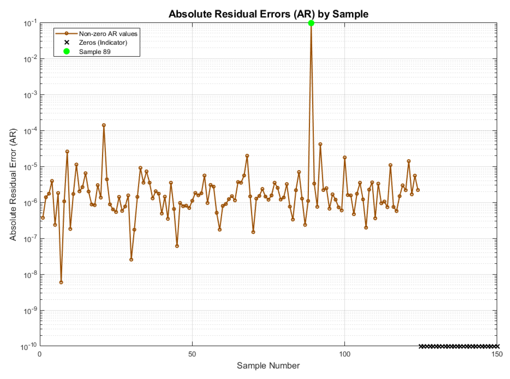
Agriculture is essential for food production and raw materials. A key aspect of this sector is harvest, the stage at which the commercial part of the plant is separated. Timely harvesting minimizes post-harvest losses, preserves product quality and optimizes production processes. Globally, a substantial amount of food is wasted, impacting food security and natural resources. To address this problem, an Adaptive Neuro-Fuzzy Inference System was developed to predict timely harvesting in crops. Stevia, a native plant from Brazil and Paraguay, with an annual production 100,000 to 200,000 tons and a market of 400 million dollars, is the focus of this study. The system considers soil pH, Brix Degrees and leaf colorimetry as inputs. The output is binary: 1 indicates timely harvest and 0 indicates no timely harvest. To assess its performance, Leave One Out Cross Validation was used, obtaining an r² of 0.99965 and a Residual Absolute Error of 0.00064305, demonstrating its accuracy and robustness. In addition, an interactive application that allows farmers to evaluate crop status and optimize decision making was developed.
Keywords:
1. Introduction
2. Materials and Methods
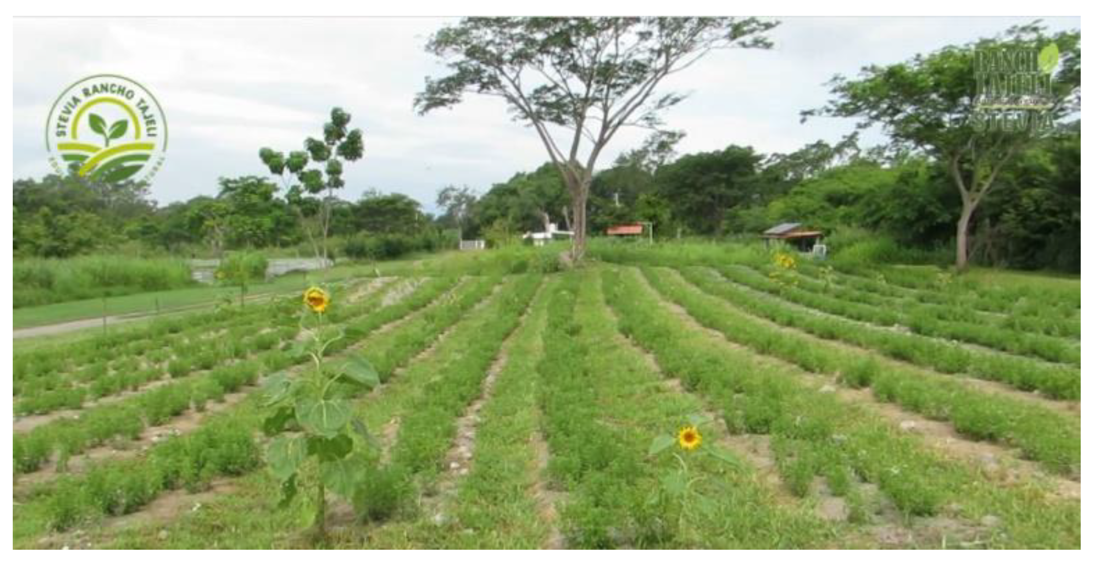
2.1. Study Area
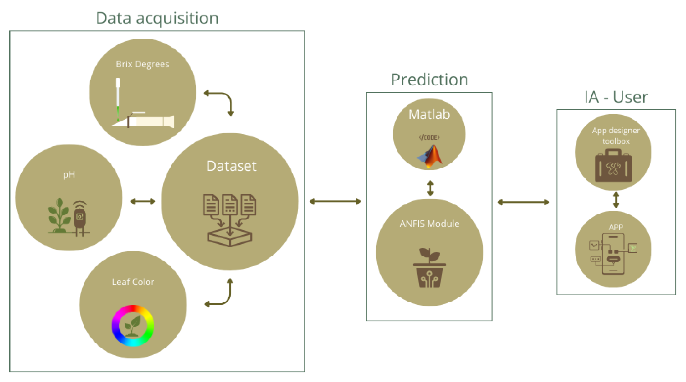
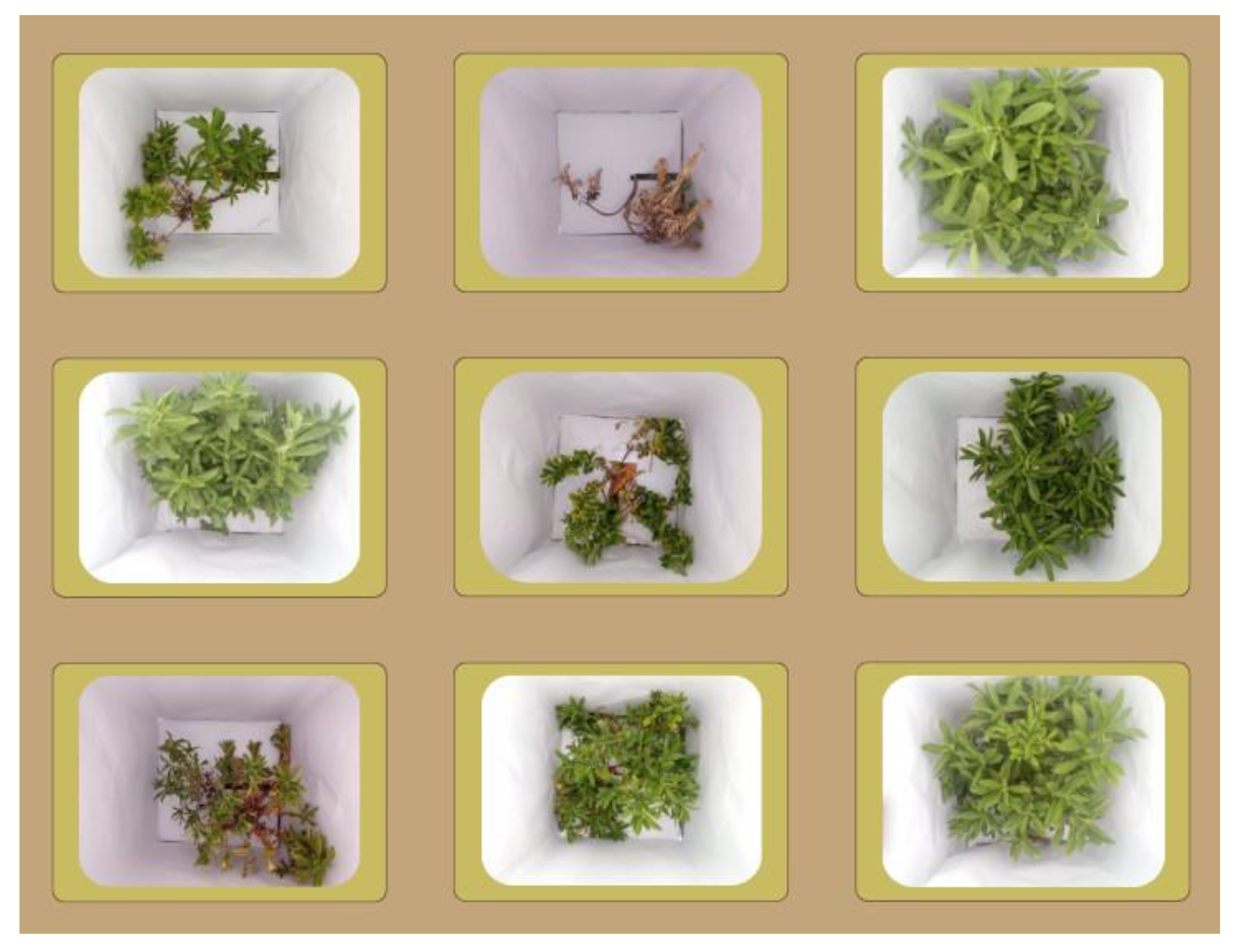
2.2. Dataset
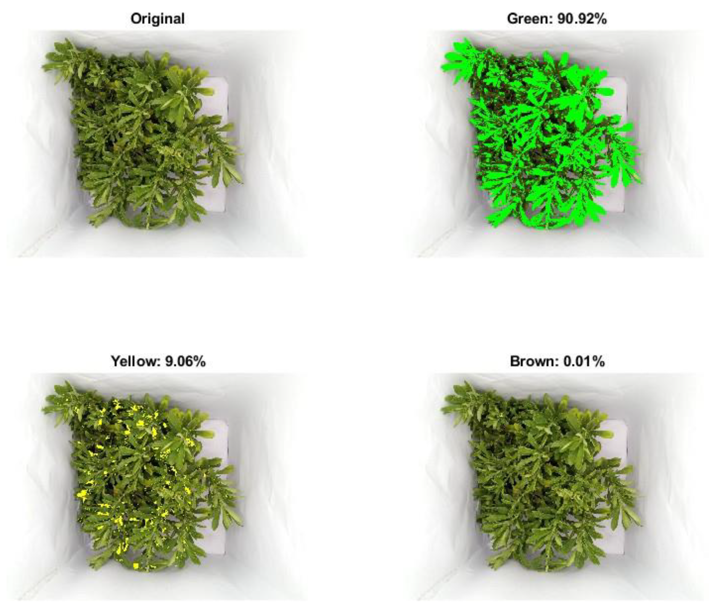
- Values obtained after subjecting crop images to processing using Binary Masks (BM) to obtain color percentages in Hue, Saturation, Value (HSV) format and then performing cluster classification using k-means algorithm as a grouping method.
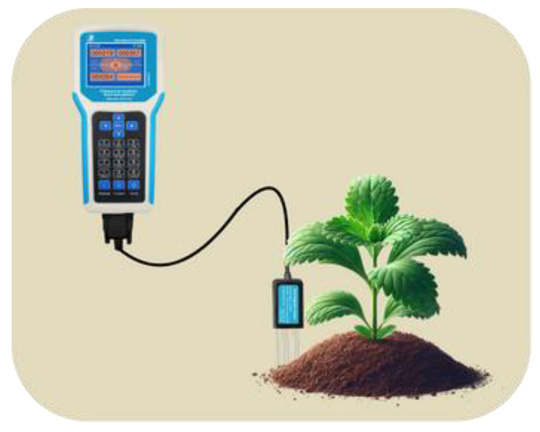
- pH values collected from soil in the study area.
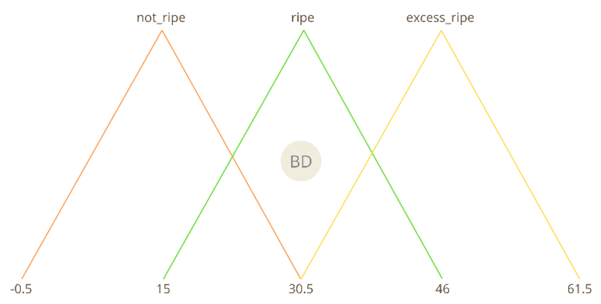
- BD values obtained from leaf samples taken from each Stevia plant.
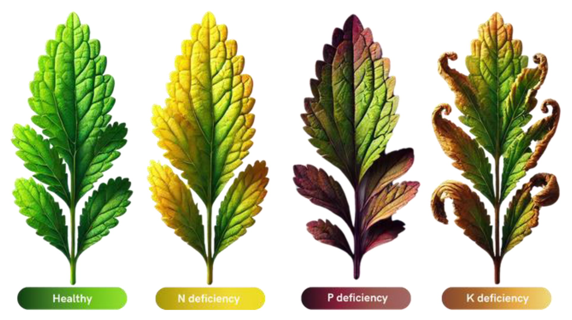
2.2.1. Image Processing for Leaf Colorimetry
- H (Hue): Specifies the hue of the color (0° to 360° mapped from [0,1] in MATLAB).
- S (Saturation): Indicates color purity [0 to 1].
- V (Value): Indicates the brightness or intensity [0 to 1].
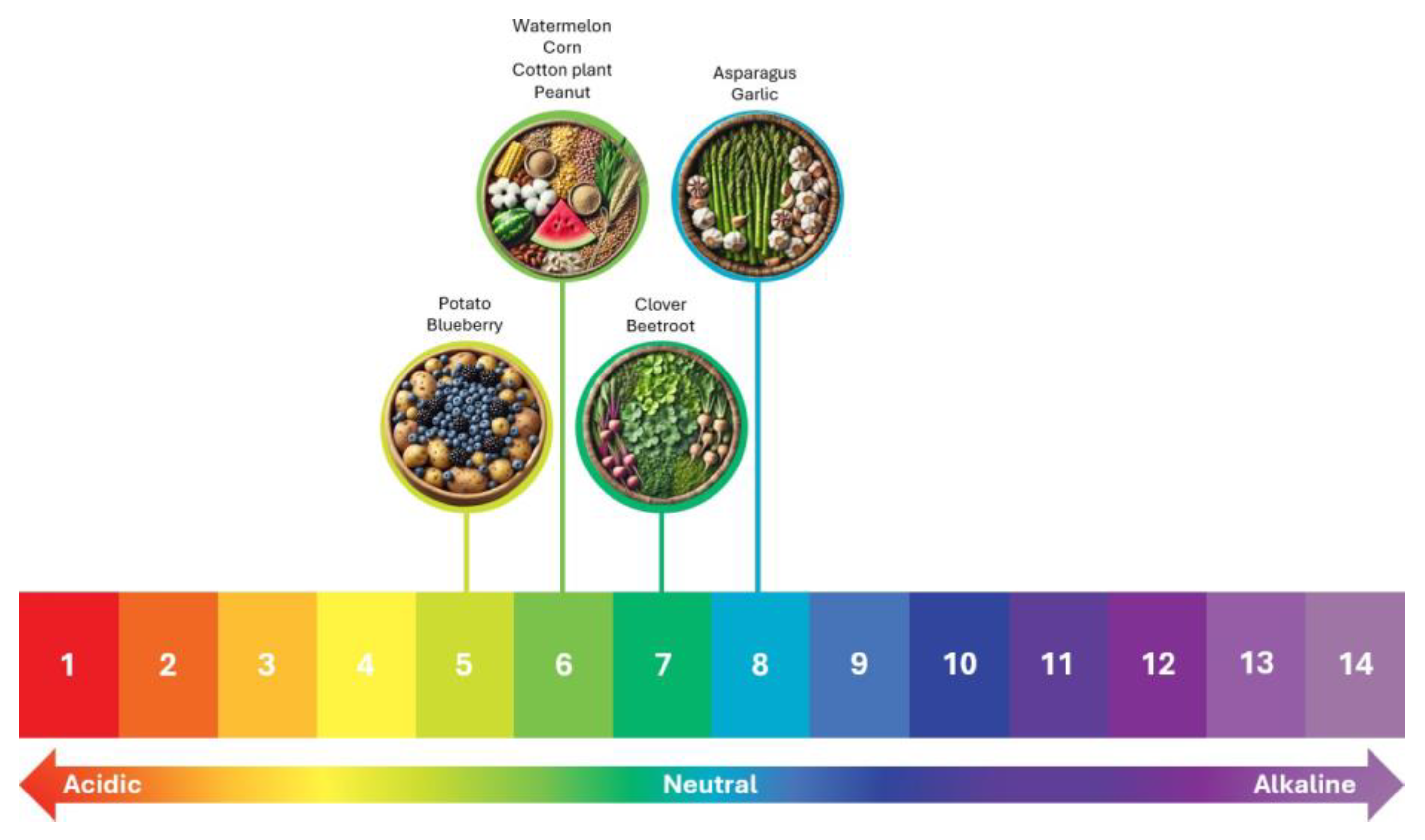
2.2.2. pH
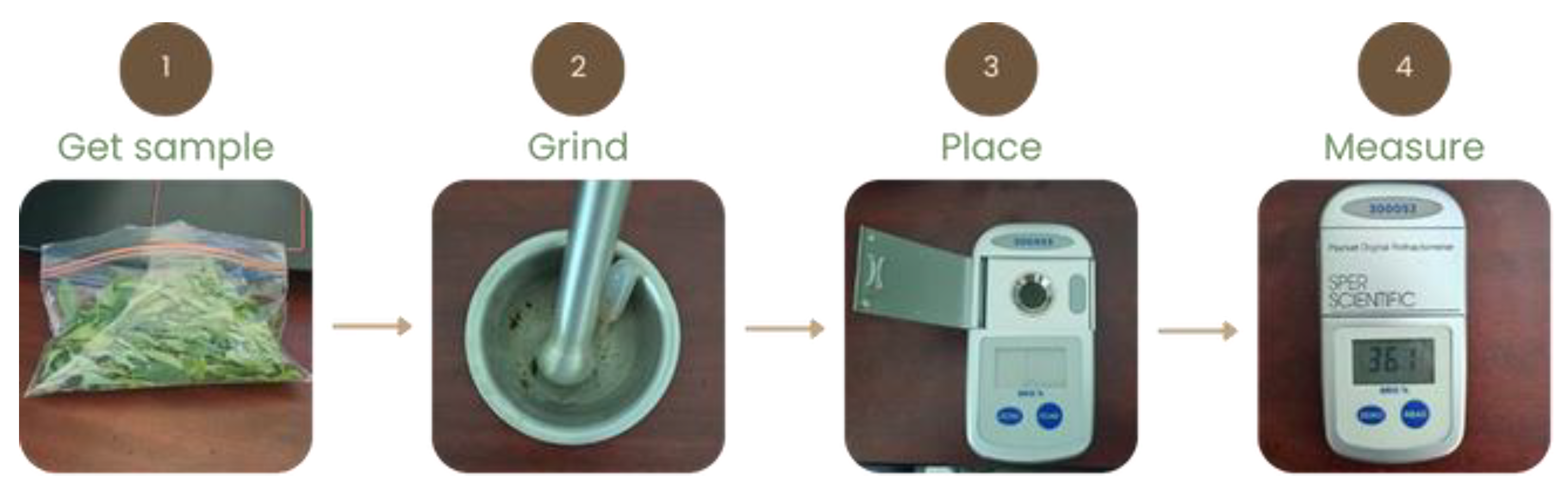
2.2.3. Brix Degrees
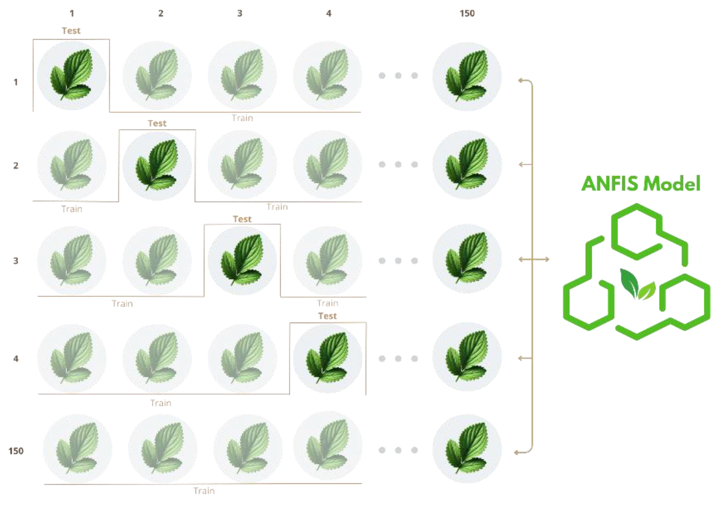
2.3. ANFIS Modeling
2.3.1. Artificial Neuronal Network (ANN)
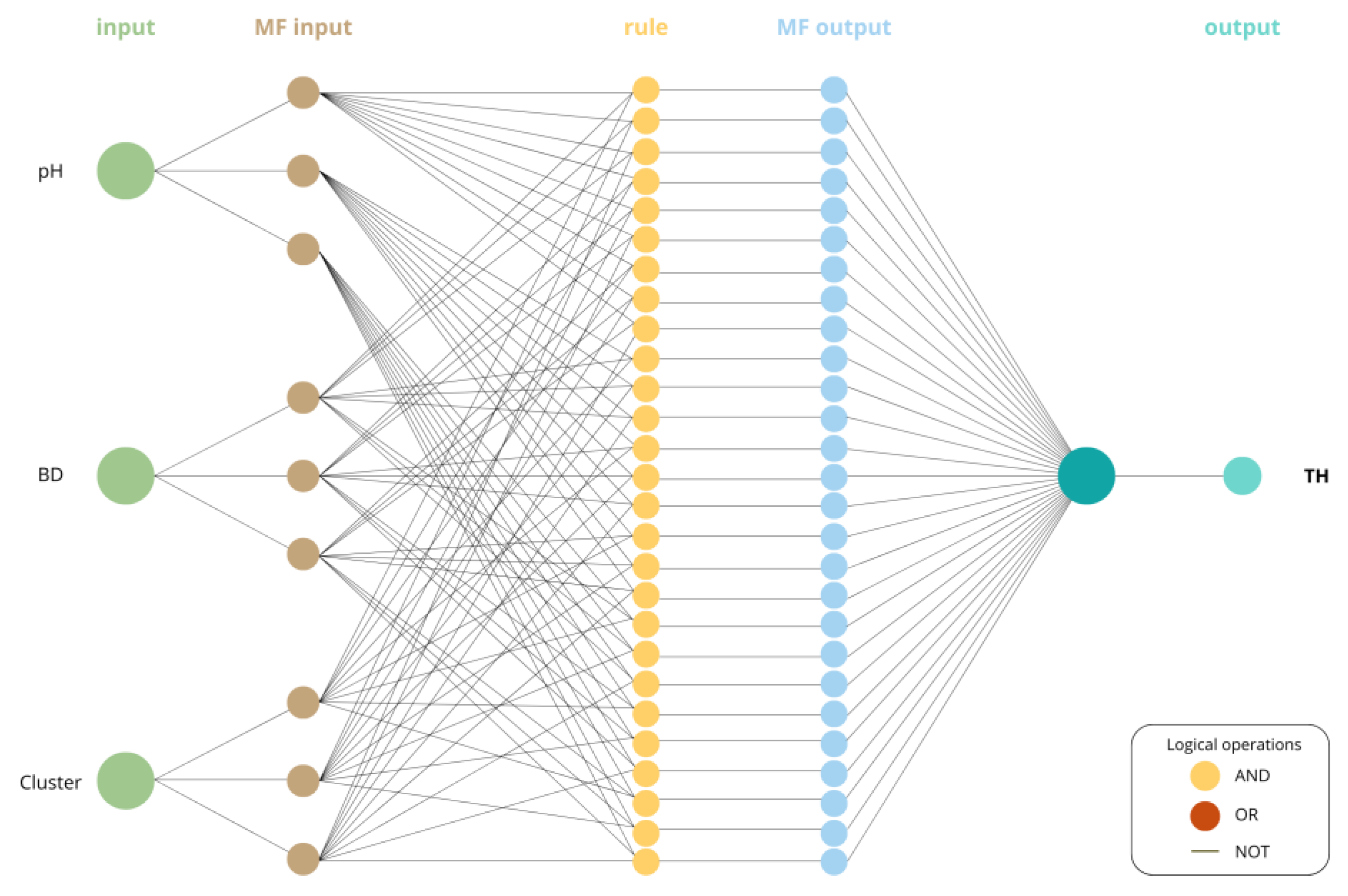
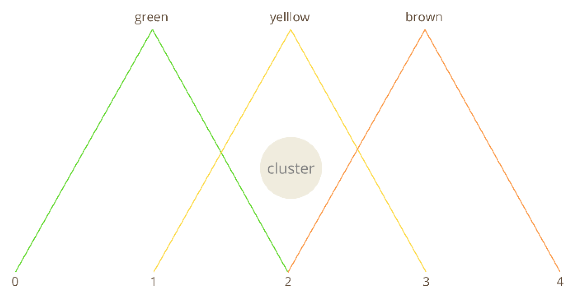
2.3.2. Fuzzy Inference System (FIS)
- Inputs:
- 2.
- Output:
- 3.
- Fuzzy Rules (FR):
2.3.3. ANFIS Model Summary
2.4. Timely Harvest Prediction Algorithm
| Algorithm 1 Timely Harvest prediction |
| Read |
| Assign inputs |
| Assign output |
| Initialize: |
| n ← number of samples. |
| absolute_residuals ← vector of size n. |
| epoch_number ← 10. |
| mf_type ← ’trimf’. |
| For: i = 1 to n |
| Split data: train_inputs, train_outputs, test_input, test_output. |
| Create initial model: fismat ← genfis1(training_data, 3, mf_type). |
| Train ANFIS model: fismat_trained ← |
| anfis(training_data, fismat, epoch_number). |
| Predict: predicted_output ← evalfis(test_input, fismat_trained). |
| EndFor |
3. Results
3.1. Evaluation Metrics
3.1.1. Model Performance
- 1.
- Absolute Residuals (AR)
- 2.
- Leave One Out Cross Validation (LOOCV)
3.2. Performance Evaluations
3.3. Determination Coefficient (r2)
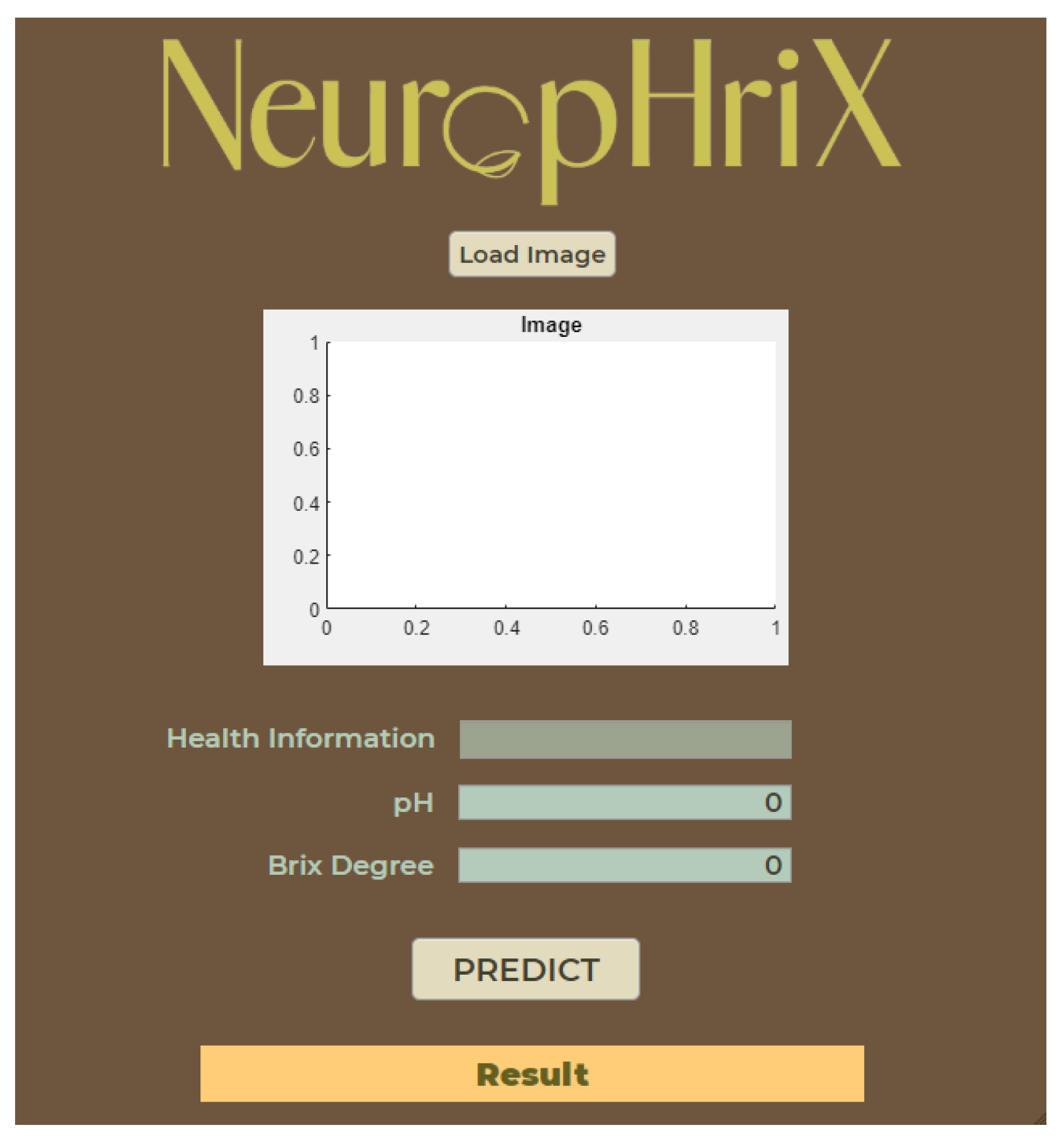
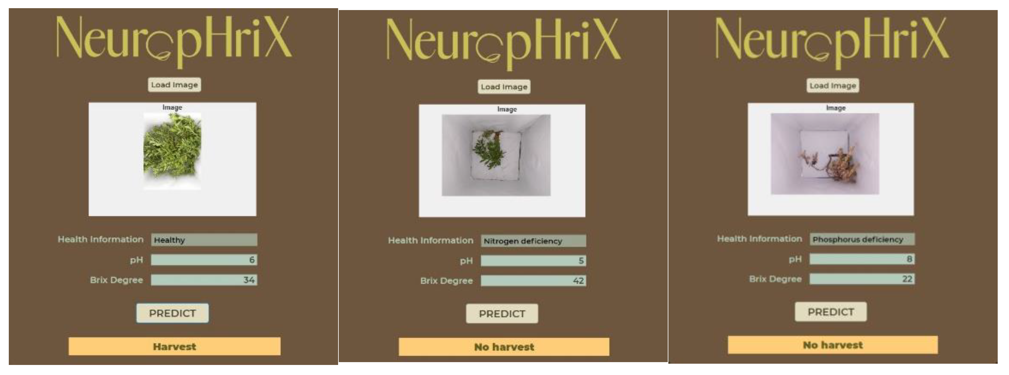
3.4. App
4. Discussion
5. Conclusions
Author Contributions
Funding
Institutional Review Board Statement
Informed Consent Statement
Data Availability Statement
Acknowledgments
Conflicts of Interest
Appendix A

| FR | i f | Antecedent | FO | Antecedent | FO | Antecedent | t h e n | Consequent | |
| 1 | not_harvest | ||||||||
| pH is acid | A N D | BD is not_ripe | A N D | cluster is 1 | |||||
| 2 | pH is acid | BD is not_ripe | cluster is 2 | not_harvest | |||||
| 3 | pH is acid | BD is not_ripe | cluster is 3 | not_harvest | |||||
| 4 | pH is acid | BD is ripe | cluster is 1 | not_harvest | |||||
| 5 | pH is acid | BD is ripe | cluster is 2 | not_harvest | |||||
| 6 | pH is acid | BD is ripe | cluster is 3 | not_harvest | |||||
| 7 | pH is acid | BD is excess_ripe | cluster is 1 | not_harvest | |||||
| 8 | pH is acid | BD is excess_ripe | cluster is 2 | not_harvest | |||||
| 9 | pH is acid | BD is excess_ripe | cluster is 3 | not_harvest | |||||
| pH is neutral | BD is not_ripe | cluster is 1 | not_harvest | ||||||
| pH is neutral | BD is not_ripe | cluster is 2 | not_harvest | ||||||
| pH is neutral | BD is not_ripe | cluster is 3 | not_harvest | ||||||
| pH is neutral | BD is ripe | cluster is 1 | harvest | ||||||
| pH is neutral | BD is ripe | cluster is 2 | not_harvest | ||||||
| pH is neutral | BD is ripe | cluster is 3 | not_harvest | ||||||
| pH is neutral | BD is excess_ripe | cluster is 1 | not_harvest | ||||||
| pH is neutral | BD is excess_ripe | cluster is 2 | not_harvest | ||||||
| pH is neutral | BD is excess_ripe | cluster is 3 | not_harvest | ||||||
| pH is alkaline | BD is not_ripe | cluster is 1 | not_harvest | ||||||
| pH is alkaline | BD is not_ripe | cluster is 2 | not_harvest | ||||||
| pH is alkaline | BD is not_ripe | cluster is 3 | not_harvest | ||||||
| pH is alkaline | BD is ripe | cluster is 1 | not_harvest | ||||||
| pH is alkaline | BD is ripe | cluster is 2 | not_harvest | ||||||
| pH is alkaline | BD is ripe | cluster is 3 | not_harvest | ||||||
| pH is alkaline | BD is excess_ripe | cluster is 1 | not_harvest | ||||||
| pH is alkaline | BD is excess_ripe | cluster is 2 | not_harvest | ||||||
| pH is alkaline | BD is excess_ripe | cluster is 3 | not_harvest |
References
- INEGI. 2024. Actividades Agrícolas. Available online: https://cuentame.inegi.org.mx/economia/primarias/agri/default.aspx?tema=E#sp (accessed on 20 January 2025).
- FAO. El estado mundial de la agricultura y la alimentación. Available online: https://www.fao.org/4/a0493s/a0493s02.htm (accessed on 20 January 2025).
- World Bank. 2024. Agriculture Overview. Available online: https://www.worldbank.org/en/topic/agriculture/overview (accessed on 20 January 2025).
- Secretaría de Agricultura y Desarrollo Rural. 2024. Hablemos de la agricultura en México. Parte 1. Available online: https://www.gob.mx/agricultura/articulos/hablemos-de-la-agricultura-en-mexico-parte-1 (accessed on 20 January 2025).
- FAO. Harvesting and Threshing. Available online: https://www.fao.org/4/t0522e/T0522E05.htm(accessed on 20 January 2025).
- FAO. Capítulo 1. Cosecha. Available online: https://www.fao.org/4/Y4893S/y4893s04.htm (accessed on 20 January 2025).
- FAO. 2020. Family Farming Knowledge Platform: Climate-Smart Agriculture and Family Farming. Available online: https://www.fao.org/family-farming/detail/en/c/1309554/ (accessed on 20 January 2025).
- Colwick, R.F. 1984. Harvesting. In Soybeans: Improvement, Production, and Uses, 2nd ed. Edited by J.R. Wilcox. Madison, WI: American Society of Agronomy, Agronomy Monograph 24, pp. 625–636. https://acsess.onlinelibrary.wiley.com/doi/abs/10.2134/agronmonogr24.c10.
- FAO. Harvesting. Available online: https://www.fao.org/4/t0522e/T0522E04.htm (accessed on 20 January 2025).
- SPRING. 2017. Farmer Nutrition School Agronomic Curriculum. Available online: https://spring-nutrition.org/sites/default/files/publications/trainingmaterials/spring_farmer_ agronomic_curriculum.pdf (accessed on 20 January 2025).
- Oklahoma State University.Swathing vs. Direct Combining. Available online: http://canola. okstate.edu/cropproduction/harvesting/swathingvsdirectcombiningv6.pdf (accessed on 20 January 2025).
- Mishra, D.; Satapathy, S. Technology adoption to reduce the harvesting losses and wastes in agriculture. Clean Technol. Environ. Policy 2021, 23, 1947–1963. [Springer] . [CrossRef]
- Erkan, M.; Dog˘ an, A. 2019. Chapter 5: Harvesting of Horticultural Commodities. In Postharvest Technology of Perishable Horticultural Commodities, edited by E.M. Yahia. Sawston, Cambridge: Woodhead Publishing, pp. 129–159. [CrossRef]
- Kaur, B.; Mansi.; Dimri, S.; Singh, J.; Mishra, S.; Chauhan, N.; Kukreti, T.; Sharma, B.; Singh, S, P.; Arora, S.; Uniyal, D.; Agrawal, Y.; Akhtar, S.; Rather, M, A.; Naik, B.; Kumar, V.; Gupta, A, K.; Rustagi, S.; Preet, M, S. Insights into the harvesting tools and equipment’s for horticultural crops: From then to now. Curr. Res. Food Sci. 2023, 6, 100430. [ScienceDirect] https://www. sciencedirect.com/science/article/pii/S2666154323003216.
- Prasad, K.; Jacob, S.; Siddiqui, M.W. 2018. Chapter 2: Fruit Maturity, Harvesting, and Quality Standards. In Preharvest Modulation of Postharvest Fruit and Vegetable Quality, edited by M.W. Siddiqui. San Diego: Academic Press, pp. 41–64. [CrossRef]
- Department of Primary Industries and Regional Development. 2024. Harvesting. Available online: https://www.agric.wa.gov.au/crops/production-postharvest/harvesting (accessed on 20 January 2025).
- Estación Experimental Agrícola de Puerto Rico. 2001 Melón: Cosecha y Manejo Poscosecha. Available online: https://www.upr.edu/eea/wp-content/uploads/sites/17/2016/03/MELON- COSECHA-Y-MANEJO-POSTCOSECHA.pdf (accessed on 20 January 2025).
- International Fertilizer Association. 2024. Precision Agriculture. Available online: https://www.fertilizer.org/science/innovation/precision-agriculture/ (accessed on 20 January 2025).
- European Commission. Precision Farming: Developing Digital Technologies for Agriculture. Available online: https://ec.europa.eu/eip/agriculture/en/digitising-agriculture/developing- digital-technologies/precision-farming-0.html (accessed on 20 January 2025).
- University of Florida.; Ampatzidis, Y. 2024. Precision Agriculture: Technology and Field Applications. Available online: https://edis.ifas.ufl.edu/publication/AE529 (accessed on 20 January 2025).
- Javaid, M.; Haleem, A.; Khan, I, H.; Suman, R. Understanding the potential applications of ArtificialIntelligence in Agriculture Sector. Advanced Agrochem 2023, 2, 70–90. [ScienceDirect] https: //www.sciencedirect.com/science/article/pii/S277323712200020X. [CrossRef]
- NASA. 2024. What Is Artificial Intelligence?. Available online: https://www.nasa.gov/what-is-artificial-intelligence (accessed on 20 January 2025).
- MDPI. 2024. Special Issue: Artificial Intelligence and Digital Agriculture. Available online: https://www.mdpi.com/journal/digital/special_issues/5F87T2J64G (accessed on 20 January 2025).
- Chakraborty, A.; Serneels, S.; Claussen, H.; Venkatasubramanian, V.; Hybrid AI Models in Chemical Engineering – A Purpose-driven Perspective; Computer Aided Chemical Engineering, 2022; pp. 925–948. [ScienceDirect] . [CrossRef]
- Chahuara Quispe, José Carlos. 2005. Neuro-fuzzy Control Applied to a Tower Crane. Bachelor’sThesis, Universidad Nacional Mayor de San Marcos, Faculty of Electronic Engineering, Lima, Peru. Available at: https://sisbib.unmsm.edu.pe/.
- García Díaz, Noel. 2014. A Multi-Layer Adaptive Neuro-Fuzzy Inference System for Estimating the Development Effort of Software Projects. Doctoral Thesis, Universidad de Guadalajara, Centro Universitario de Ciencias Económico Administrativas, Zapopan, Jalisco, Mexico.
- Abraham, A. Neuro fuzzy systems: State-of-the-art modeling techniques. [arXiv] https://arxiv.org/pdf/cs/0405011.
- Jang, J.-S.R. ANFIS: Adaptive-Network-Based Fuzzy Inference System. IEEE Transactions on Systems, Man, and Cybernetics 1993, 23, 665–685. [IEEE] . [CrossRef]
- Jithendra, T.; Basha, S.S. A Hybridized Machine Learning Approach for Predicting COVID-19 Using Adaptive Neuro-Fuzzy Inference System and Reptile Search Algorithm. Diagnostics 2023, 13, 1641. [MDPI] https://www.mdpi.com/2075-4418/13/9/1641. [CrossRef]
- Rahman, M, S.; Ali, M, H. Adaptive Neuro Fuzzy Inference System (ANFIS)-Based Control for Solving the Misalignment Problem in Vehicle-to-Vehicle Dynamic Wireless Charging Systems. Electronics 2025, 14, 507. [MDPI] https://www.mdpi.com/2079-9292/14/3/507.
- Kudelina, K.; Raja, H.A. Neuro-Fuzzy Framework for Fault Prediction in Electrical Machines via Vibration Analysis. Energies 2024, 17, 2818. [MDPI] https://www.mdpi.com/1996-1073/17/12/2818. [CrossRef]
- Wang, Y.; Zhang, N.; Chen, C.; Jiang, Y.; Liu, T. Nonlinear Adaptive Generalized Predictive Control for PH Model of Nutrient Solution in Plant Factory Based on ANFIS. Processes 2023, 11, 2317. [MDPI] https://www.mdpi.com/2227-9717/11/8/2317. [CrossRef]
- Morozov, S.; Kupriyanov, M. A Neuro-Fuzzy System for Power Supply Control. Engineering Proceedings 2023. [MDPI] https://www.mdpi.com/2673-4591/33/1/49.
- Kheioon, I, A.; Al-Sabur, R.; Sharkawy, A-N. Design and Modeling of an Intelligent Robotic Gripper Using a Cam Mechanism with Position and Force Control Using an Adaptive Neuro-Fuzzy ComputingTechnique. Automation 2025, 6, 4. [MDPI] https://www.mdpi.com/2673-4052/6/1/4.
- Mustafa, R.; Samui, P.; Kumari, S. Reliability Analysis of Gravity Retaining Wall Using Hybrid ANFIS. Infrastructures 2022, 7, 121. [MDPI] https://www.mdpi.com/2412-3811/7/9/121. [CrossRef]
- Kumar, M, S.; Rajamani, D.; Nasr, E, A.; Balasubramanian, E.; Mohamed, H.; Astarita, A. A Hybrid Approach of ANFIS—Artificial Bee Colony Algorithm for Intelligent Modeling and Optimization of Plasma Arc Cutting on Monel™ 400 Alloy. Materials 2021, 14, 6373. [MDPI] https://www.mdpi.com/1996-1944/14/21/6373.
- Luo, Y.; Wang, X.; Wang, Q.; Chen, Y. Illuminant Estimation Using Adaptive Neuro-Fuzzy Inference System. Applied Sciences 2021, 11, 9936. [MDPI] https://www.mdpi.com/2076-3417/11/21/9936. [CrossRef]
- Taylan, O.; Alkabaa, A.S.; Alamoudi, M.; Basahel, A.; Balubaid, M.; Andejany, M.; Alidrisi, H. Air Quality Modeling for Sustainable Clean Environment Using ANFIS and Machine Learning Approaches. Atmosphere 2021, 12, 713. [MDPI] https://www.mdpi.com/2073-4433/12/6/713. [CrossRef]
- Bulus, H, N. Adaptive Neuro-Fuzzy Inference System and Artificial Neural Network Models for Predicting Time-Dependent Moisture Levels in Hazelnut Shells (Corylus avellana L.) and Prina (Oleae europaeae L.). Processes 2024, 12, 1703. [MDPI] https://www.mdpi.com/2227-9717/12/8/1703.
- Nezhad, H, L.; Sharabiani, V, R.; Tarighi, J.; Tahmasebi, M.; Taghinezhad, E.; Szumny, A. textitEn- ergy Flow Analysis in Oilseed Sunflower Farms and Modeling with Artificial Neural Networks as Compared to Adaptive Neuro-Fuzzy Inference Systems (Case Study: Khoy County). Energies 2024, 17, 2795. [MDPI] https://www.mdpi.com/1996-1073/17/11/2795. [CrossRef]
- Sunori, S, K.; Pant, J.; Maurya, S.; Mittal, A.; Arora, S.; Juneja, P. Neuro-Fuzzy based Prediction of pH Value of Soil of Uttarakhand. IEEE Xplore 2021. [IEEE] https://ieeexplore.ieee.org/document/9452814/.
- Sulistyaningrum, D.R.; Setiyono, B.; Tsaqif, M.; Hakam, A. Adaptive Neuro-Fuzzy Inference System for Identification of Rice Plant Diseases. AIP Conference Proceedings 2024, 3029, 060003. [AIP] https://pubs.aip.org/aip/acp/article/3029/1/060003/3306412.
- García-Rodríguez, L, C.; Morales-Viscaya, J, A.; Prado-Olivarez, J.; Barranco-Gutiérrez, A, I.; Padilla-Medina, J, A.; Espinosa-Calderón, A. Fuzzy Mathematical Model of Photosynthesis in Jalapeño Pepper. Agriculture 2024, 14, 909. [MDPI] https://www.mdpi.com/2077-0472/14/6/909.
- Remya, S. An adaptive neuro-fuzzy inference system to monitor and manage the soil quality to improve sustainable farming in agriculture. Soft Computing 2022, 26, 13119–13132. [Springer] https://link.springer.com/article/10.1007/s00500-022-06832-3. [CrossRef]
- Vincentdo, V.; Surantha, N. Nutrient Film Technique-Based Hydroponic Monitoring and Controlling System Using ANFIS. Electronics 2023, 12, 1446. [MDPI] https://www.mdpi.com/2079-9292/12/6/1446. [CrossRef]
- Tian, X.; Meng, X.; Wu, Q.; Chen, Y.; Pan, J. Identification of Tomato Leaf Diseases based on a Deep Neuro-fuzzy Network. Journal of The Institution of Engineers (India): Series A 2022, 103, 695–706.[Springer] https://link.springer.com/article/10.1007/s40030-022-00642-4. [CrossRef]
- Boonyopakorn, P.; Bualeard, P. Applying Neuro Fuzzy System to Analyze Durian Minerals within Soil for Precision Agriculture. IEEE Access 2020. [IEEE] https://ieeexplore.ieee.org/abstract/document/9158093.
- Abbaspour-Gilandeh, M.; Abbaspour-Gilandeh, Y.Modelling soil compaction of agricultural soils using fuzzy logic approach and adaptive neuro-fuzzy inference system (ANFIS) approaches. Modeling Earth Systems and Environment 2018, 5, 13-20. [Springer] https://link.springer.com/article/10.1007/s40808-018-0514-1. [CrossRef]
- Rezaei, M.; Rohani, A.; Lawson, S, S. Using an Adaptive Neuro-fuzzy Interface System (ANFIS) to Estimate Walnut Kernel Quality and Percentage from the Morphological Features of Leaves and Nuts.Erwerbs-Obstbau 2022, 64, 611-620. [Springer] . [CrossRef]
- Adeyi, O.; Adeyi, A.J.; Oke, E.O.; Ajayi, O.K.; Oyelami, S.; Otolorin, J.A.; Areghan, S.E.; Isola, B.F. Adaptive neuro fuzzy inference system modeling of Synsepalum dulcificum L. drying characteristics and sensitivity analysis of the drying factors. Scientific Reports 2022, 12, 13261. [Nature] https://www.nature.com/articles/s41598-022-17705-y. [CrossRef]
- Abraham, E, R.; Mendes-dos-Reis, J, G.; de-Souza, A, E.; Paulieli, A. Neuro-Fuzzy System for the Evaluation of Soya Production and Demand in Brazilian Ports. In Advances in Production Management Systems. Production Management for the Factory of the Future, 2019; pp. 87–94. [Springer] https://link.springer.com/chapter/10.1007/978-3-030-30000-5_11.
- Phaiboon, S.; Phokharatkul, P. Applying an Adaptive Neuro-Fuzzy Inference System to Path Loss Prediction in a Ruby Mango Plantation. Journal of Sensor and Actuator Networks 2023, 12, 71. [MDPI] https://www.mdpi.com/2224-2708/12/5/71. [CrossRef]
- Hobart, M.; Schirrmann, M.; Abubakari, A-H.; Badu-Marfo, G.; Kraatz, S.; Zare, M. Drought Monitoring and Prediction in Agriculture: Employing Earth Observation Data, Climate Scenarios and Data Driven Methods; a Case Study: Mango Orchard in Tamale, Ghana. Remote Sensing 2024, 16, 1942. [MDPI] https://www.mdpi.com/2072-4292/16/11/1942. [CrossRef]
- Chughtai, M.F.J.; Pasha, I.; Zahoor, T.; Khaliq, A.; Ahsan, S.; Wu, Z.; Nadeem, M.; Mehmood, T.; Amir, R, M.; Yasmin, I.; Liaqat, A.; Tanweer, S.Nutritional and therapeutic perspectives of Stevia rebaudiana as emerging sweetener; a way forward for sweetener industry. CyTA-Jounal of Food 2020, textit18, 1. [Taylor Francis] . [CrossRef]
- S´niegowska, J.; Biesiada, A.Effect of Spacing on Growth, Yield and Chemical Composition of Stevia Plants (Stevia rebaudiana Bert.). Applied Sciences 2024, 14, 5153. [MDPI] https://www.mdpi.com/2076-3417/14/12/5153.
- Cámara de Diputados. 2018. La Producción de Stevia en México: Una Alternativa Saludable y Sustentable. Available online: https://portalhcd.diputados.gob.mx/PortalWeb/Micrositios/69 e0b07c-5ceb-430c-8737-fa9d2e651750/92Estevia.pdf (accessed on 20 January 2025).
- Secretaría de Agricultura y Desarrollo Rural. En México, la Stevia Conquista el Mercado de los Edulcorantes. Available online: https://www.gob.mx/agricultura/es/articulos/en-mexico-la- stevia-conquista-el-mercado-de-los-edulcorantes (accessed on 20 January 2025).
- Vejar-Cortés, A-P.; García-Díaz, N.; Soriano-Equigua L.; Ruiz-Tadeo, A-C.; Álvarez-Flores, J-L. Determination of Crop Soil Quality for Stevia rebaudiana Bertoni Morita II Using a Fuzzy Logic Model and a Wireless Sensor Network. Applied Sciences 2023, 13, 9507. [MDPI] https://www.mdpi.com/2076-3417/13/17/9507. [CrossRef]
- Aptus Holland. 2022. Quality Factor: Brix. Available online: https://aptus-holland.com/quality-factor-brix/ (accessed on 20 January 2025).
- Zhang, Y.-Y.; Wu, W.; Liu, H. Factors affecting variations of soil pH in different horizons in hilly regions. PLoS ONE 2019, 14, e0218563. [Public Library of Science] . [CrossRef]
- University of Connecticut. 2018. Soil pH: The Master Variable. Available online: https: //publications.extension.uconn.edu/2018/12/07/soil-ph-the-master-variable/#:~:text=Mineral%20soil%20pH%20values%20generally,content%20also%20influence%20soil%20pH. (accessed on 20 January 2025).
- FAO. 2021. ¿Qué es el pH del suelo?. Available online: https://openknowledge.fao.org/server/api/core/bitstreams/e434293f-c9d1-4585-a799-b7c9107ea64e/content (accessed on 20 January 2025).
- The Ohio State University. 2013. Soil pH and Lime Recommendations. Available online: https://ohioline.osu.edu/factsheet/HYG-1651 (accessed on 20 January 2025).
- Jaywant, S.A.; Singh, H.; Arif, K.M. Sensors and Instruments for Brix Measurement: A Review. Sensors 2022, 22, 2290. [MDPI] https://www.mdpi.com/1424-8220/22/6/2290. [CrossRef]
- Miyakawa, M.; Hoshina, S. A self-supporting gel phantom used for visualization and/or measurement of the three-dimensional distribution of SAR. 2002. [IEEE] https://ieeexplore.ieee.org/document/1032672.
- Siregar, R, R, A.; Seminar, K, B.; Wahjuni, S.; Santosa, E.; Sikumbang, H. Backpropagation Algorithm to Detect The Color of The Leaf to Determine The Need for Nutrients 2023. [IEEE] https: //ieeexplore.ieee.org/document/10326726.
- Begum, S, S.; Yannam, A.; Chowdary, M.C, C.; Devi, T, R.; Nallamothu, V, P.; Jahnavi, Y. Deep Learning-based Nutrient Deficiency symptoms in plant leaves using Digital Images. 2024. [IEEE] https://ieeexplore.ieee.org/document/10435129.
- Veazie, P.; Cockson P.; Henry, J.; Perkins-Veazie, P.; Whipker, B. Characterization of Nutrient Disorders and Impacts on Chlorophyll and Anthocyanin Concentration of Brassica rapa var. Chinensis. Agriculture 2020, 10, 461. [MDPI] https://www.mdpi.com/2077-0472/10/10/461. [CrossRef]
- Rancho Tajeli. 2023. Rancho Tajeli . Available online: https://www.ranchotajeli.com (accessed on 20 January 2025).
- Hiremath, S.B.; Shet, R.; Patil, N.; Iyer, N. Sensor Based On-the-Go Detection of Macro Nutrients for Agricultural Crops. Advances in Science, Technology and Engineering Systems Journal 2020, 5, 128–134. [ASTESJ] http://dx.doi.org/10.25046/aj050117.
- Hu, S.; Bian, Y.; Chen, B.; Song, H.; Zhang, K. Language-Guided Semantic Clustering for Remote Sensing Change Detection. Sensors 2024, 24, 7887. [MDPI] https://www.mdpi.com/1424-8220/24/24/7887. [CrossRef]
- Jaszcz A.; Włodarczyk-Sielicka, M.; Stateczny, A.; Połap, D.; Garczyn´ska, I. Automated Shoreline Segmentation in Satellite Imagery Using USV Measurements. Remote Sensing 2024, 16, 4457. [MDPI] https://www.mdpi.com/2072-4292/16/23/4457.
- Li, X.; Qin, J.; Long, Y. Urban Architectural Color Evaluation: A Cognitive Framework Combining Machine Learning and Human Perception. Buildings 2024, 14, 3901. [MDPI] https://www.mdpi.com/2075-5309/14/12/3901. [CrossRef]
- Zhi, J.; Li, L.; Zhu, H.; Li, Z.; Wu, M.; Dong, R.; Cao, X.; Liu, W.; Qu, L.; Song, X.; Shi, L. Comparison of Deep Learning Models and Feature Schemes for Detecting Pine Wilt Diseased Trees. Forests 2024, 15, 1706. [MDPI] https://www.mdpi.com/1999-4907/15/10/1706. [CrossRef]
- Zbiljic´, M.; Lakušic´, D.; Šatovic´, Z.; Liber, Z.; Kuzmanovic´, N. Patterns of Genetic and Morphological Variability of Teucrium montanum sensu lato (Lamiaceae) on the Balkan Peninsula. Plants 2024, 13, 3596. [MDPI] https://www.mdpi.com/2223-7747/13/24/3596.
- Raddad, Y.; Hasasneh, A.; Abdallah, O.; Rishmawi, C.; Qutob, N. Integrating Statistical Methods and Machine Learning Techniques to Analyze and Classify COVID-19 Symptom Severity. Big Data and Cognitive Computing 2024, 8, 192. [MDPI] https://www.mdpi.com/2504-2289/8/12/192. [CrossRef]
- Yoon, C.; Cho, S.; Lee, Y. Extending WSN Lifetime with Enhanced LEACH Protocol in Autonomous Vehicle Using Improved K-Means and Advanced Cluster Configuration Algorithms. Applied Sciences 2024, 14, 11720. [MDPI] https://www.mdpi.com/2076-3417/14/24/11720. [CrossRef]
- Zhang, S.; Liu, H.; Meng, Z. Agricultural Machinery Movement Trajectory Recognition Method Based on Two-Stage Joint Clustering. Agriculture 2024, 14, 2294. [MDPI] https://www.mdpi.com/2077-0472/14/12/2294. [CrossRef]
- Huang, L.; Qiu, M.; Xu, A.; Zhu, J. UAV Imagery for Automatic Multi-Element Recognition and Detection of Road Traffic Elements. Aerospace 2022, 9, 198. [MDPI] https://www.mdpi.com/2226-4310/9/4/198. [CrossRef]
- JXCT. 2025. Portable Soil Moisture Detector. Available online: https://jxctsmart.com/product/ portable-soil-moisture-detector (accessed on 20 January 2025).
- Sper Scientific. 2025. Official Website. Available online: https://www.sperdirect.com (accessed on 20 January 2025).
- Sper Scientific. Pocket Digital Refractometers. 300050-300055. Instruction Manual. Available online: https://www.instrumentchoice.com.au/attachment/download/79122/5f62c3eaebab9194748554.pdf?srsltid=AfmBOoo-8l2AcbwNiQDOVtrCfX5ZIxR3-V8-OdBC8muwqYVP74Tk_Jbv (accessed on 20 January 2025).
- Xu, B.; Su, J.; Dale, D.S.; Watson, M.D. Cotton Color Grading with a Neural Network. Textile Research Journal 2000, 70. [SAGE] . [CrossRef]
- Alotaibi, M.A. Machine Learning Approach for Short-Term Load Forecasting Using Deep Neural Network. Energies 2022, 15, 6261. [MDPI] https://www.mdpi.com/1996-1073/15/17/6261. [CrossRef]
- Silhavy, R.; Silhavy, P.; Prokopova, Z. Using Actors and Use Cases for Software Size Estimation. Electronics 2021, 10, 592. [MDPI] https://www.mdpi.com/2079-9292/10/5/592. [CrossRef]
- Lopez-Martin, C.; Villuendas-Rey, Y.; Azzeh, M.; Nassif, A, B.; Banitaan, S. Transformed k-nearest neighborhood output distance minimization for predicting the defect density of software projects. Journal of Systems and Software 2020, 167, 110592. [Elsevier] . [CrossRef]
- Garcia-Diaz, N.; Verduzco-Ramírez, A.; García-Virgen Juan.; Muñoz, L. Applying Absolute Residuals as Evaluation Criterion for Estimating the Development Time of Software Projects by Means of a Neuro-Fuzzy Approach. Journal of Information Systems Engineering Management 2016. [Lectito] . [CrossRef]
- Liu, H.; Zhu, Q.; Xia, X.; Li, M.; Huang, D. Multi-Feature Optimization Study of Soil Total Nitrogen Content Detection Based on Thermal Cracking and Artificial Olfactory System. Agriculture 2021, 12, 37. [MDPI] https://www.mdpi.com/2077-0472/12/1/37. [CrossRef]
- Liu, W.; Wang, J.; Hu, Y.; Ma, T.; Otgonbayar, M.; Li, C.; Li, Y.; Yang J. Mapping Shrub Biomass 716 at 10 m Resolution by Integrating Field Measurements, Unmanned Aerial Vehicles, and Multi-Source Satellite Observations. Remote Sensing 2024, 16, 3095. [MDPI] https://www.mdpi.com/2072-4292/16/16/3095.
- Khatri, U.; Kwon, G-R. Classification of Alzheimer’s Disease and Mild-Cognitive Impairment Based on High-Order Dynamic Functional Connectivity at Different Frequency Bands. Mathematics 2022, 10, 805. [MDPI] https://www.mdpi.com/2227-7390/10/5/805. [CrossRef]
- Gomez, D.; Salvador, P.; Rodrigo, J, F.; Gil, J. Detecting Sensitive Spectral Bands and VegetationIndices for Potato Yield Using Handheld Spectroradiometer Data. Plants 2024, 13, 3436. [MDPI] https://www.mdpi.com/2223-7747/13/23/3436. [CrossRef]
- Moore D.S.; McCabe G.P.; Craig, B.A. 2009. Introduction to the Practice of Statistics. 6ª ed. ISBN-13: 978-1-4292-1623-4.
- Humphrey, W.S. 1995. A Discipline for Software Engineering. 1ª ed. Reading, MA: Addison-Wesley Professional. ISBN: 978- 0201546101.
- Wang, Y.; Li, T.; Chen, T.; Zhang, X.; Taha, M.F.; Yang, N.; Mao, H.; Shi, Q. Cucumber Downy Mildew Disease Prediction Using a CNN-LSTM Approach. Agriculture 2024, 14, 1155. [MDPI]https://www.mdpi.com/2077-0472/14/7/1155. [CrossRef]
- Dai, J.; Pan, L.; Deng, Y.; Wan, Z.; Xia, R. Modified SWAT Model for Agricultural Watershed in Karst Area of Southwest China. Agriculture 2025, 15, 192. [MDPI] https://www.mdpi.com/2077-0472/15/2/192. [CrossRef]
- Shao, T.; Xu, X.; Su, Y. Evaluation and Prediction of Agricultural Water Use Efficiency in the Jianghan Plain Based on the Tent-SSA-BPNN Model. Agriculture 2025, 15, 140. [MDPI] https://www.mdpi.com/2077-0472/15/2/140. [CrossRef]
- Du, L.; Luo, S. Spectral-Frequency Conversion Derived from Hyperspectral Data Combined with Deep Learning for Estimating Chlorophyll Content in Rice. Agriculture 2024, 14, 1186. [MDPI] https://www.mdpi.com/2077-0472/14/7/1186. [CrossRef]
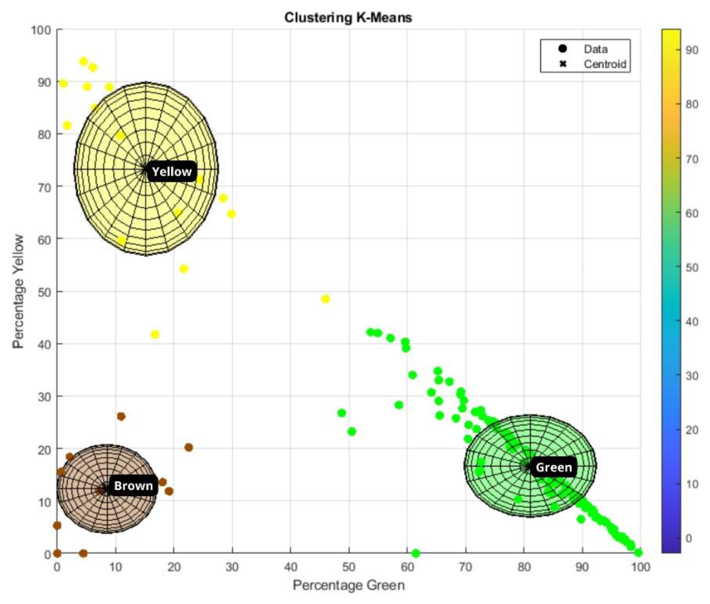
| Cluster: Color | ||
| 1: Green | 2: Yellow | 3: Brown |
| Image | %Green | %Yellow | %Brown | Cluster |
| 120.jpg | 99.5584 | 0.14344 | 0.29818 | 1 |
| 75.jpg | 10.8477 | 79.6597 | 9.94261 | 2 |
| 76.jpg | 4.44868 | 0 | 95.5513 | 3 |
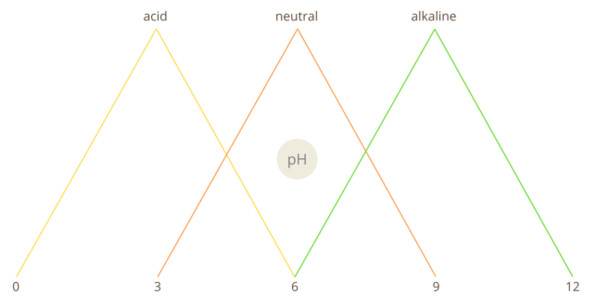
| Variable Range | Indicator | |
| pH 3–9 acid | neutral | alkaline |
| [0 3 6] | [3 6 9] | [6 9 12] |
| BD 15–46 not_ripe | ripe | excess_ripe |
| [-0.5 15 30.5] | [15 30.5 46] | [30.5 46 61.5] |
| Cluster 1–3 green | yellow | brown |
| [0 1 2] | [1 2 3] | [2 3 4] |
| Variable Range | Indicator | |
| Harvest 0–1 |
not_harvest [0] |
harvest [1] |
| FR | i f | Antecedent | FO | Antecedent | FO | Antecedent | t h e n | Consequent | |
| 1 | not_harvest | ||||||||
| pH is acid | A N D | BD is not_ripe | A N D | cluster is 1 | |||||
| 2 | pH is acid | BD is ripe | cluster is 2 | not_harvest | |||||
| 3 | pH is acid | BD is excess_ripe | cluster is 3 | not_harvest | |||||
| 4 | pH is neutral | BD is not_ripe | cluster is 1 | not_harvest | |||||
| 5 | pH is neutral | BD is ripe | cluster is 2 | not_harvest | |||||
| 6 | pH is neutral | BD is excess_ripe | cluster is 3 | not_harvest | |||||
| 7 | pH is alkaline | BD is not_ripe | cluster is 1 | not_harvest | |||||
| 8 | pH is alkaline | BD is ripe | cluster is 2 | not_harvest | |||||
| 9 | pH is alkaline | BD is excess_ripe | cluster is 3 | not_harvest |
| Training Features | |||
| Number of inputs | 3 | ||
| Number of outputs | 1 | ||
| Number of training epochs | |||
| MFs input | 3 per input variable | ||
| Number of FR | |||
| Input FM Parameters | |||
| Input 1 | MF 1 (acid): trimf - Range: [0 3 6] MF 2 (neutral): trimf - Range: [3 6 9] MF 3 (alkaline): trimf - Range: [6 9 ] |
||
| Input 2 | MF 1 (not_ripe): trimf - Range: [-3.5 13 29.5] MF 2 (ripe): trimf - Range: [13 29.5 46] MF 3 (excess ripe): trimf - Range: [29.5 46 62.5] |
||
| Input 3 | MF 1 (1): trimf - Range: [0 1 2] MF 2 (2): trimf - Range: [1 2 3] MF 3 (3): trimf - Range: [2 3 4] |
||
| Output Parameters | |||
| Output: Constant type | harvest: [1] not_harvest: [0] |
||
| Neuronal Network Structure | |||
| Number of layers | 5 | ||
| Number of neurons in layer 1 (input MF) | 9 | ||
| Number of neurons in layer 2 (RF) | 27 | ||
| Layer 3 | Standardization | ||
| Layer 4 | Linear functions | ||
| Layer 5 | Weighted sum | ||
Disclaimer/Publisher’s Note: The statements, opinions and data contained in all publications are solely those of the individual author(s) and contributor(s) and not of MDPI and/or the editor(s). MDPI and/or the editor(s) disclaim responsibility for any injury to people or property resulting from any ideas, methods, instructions or products referred to in the content. |
© 2025 by the authors. Licensee MDPI, Basel, Switzerland. This article is an open access article distributed under the terms and conditions of the Creative Commons Attribution (CC BY) license (http://creativecommons.org/licenses/by/4.0/).


