
Submitted:
19 July 2023
Posted:
20 July 2023
You are already at the latest version
Abstract
Stevia Rebaudiana Bertoni Morita II, a perennial plant native to Paraguay and Brazil, is also widely cultivated in the state of Colima, Mexico, for its use as a sweetener in food and beverages. The op-timization of soil parameters is crucial for maximizing biomass production and stevioside levels in stevia crops. This research presents the development and implementation of a monitoring system to track essential soil parameters, including pH, temperature, humidity, electrical conductivity, ni-trogen, phosphorus, and potassium. The system employs a wireless sensor network to collect qua-si-real-time data, which is transmitted and stored in a web-based platform. A Mamdani-type fuzzy logic model is utilized to process the collected data and provide to farmers an integrated assessment of soil quality. By comparing the quality data output of the fuzzy logic model with a line-ar-regression model, the system demonstrated acceptable performance, with a determination coef-ficient of 0.532 for random data and 0.906 for gathered measurements. The system enables farmers to gain insights into the soil quality of their stevia crops and empowers them to take preventive and corrective actions to improve the soil quality specifically for stevia crops.
Keywords:
Stevia Rebaudiana
; soil quality
; monitoring system
; fuzzy logic
; wireless sensor network
; Mamdani
1. Introduction
Stevia, scientifically known as Stevia Rebaudiana Bertoni, is a perennial plant that has been used for centuries as a natural sweetener and for medicinal purposes. It belongs to the Asteraceae family and is native to the northern regions of Paraguay and southern Brazil [1]. Stevia Morita II, a specific variety of Stevia Rebaudiana Bertoni, was initially cultivated in Japan by Toyosigue Morita. This variant is characterized by its higher production of dried leaves and improved chemical composition, making it highly desirable for being up to 300 times sweeter than sucrose [2,3,4].
Stevia's importance lies in its potential as a non-caloric sweetener and its use as a natural medicine. Its cultivation and usage have not only garnered attention for its economic value but also for its potential contribution to healthier dietary choices and the fight against chronic noncommunicable diseases such as obesity, diabetes, and cardiovascular diseases [3]. The chemical composition and steviol glycoside content in stevia leaves can vary depending on the country of cultivation, making it crucial to compare and understand these variations [1].
Stevia holds significant economic significance globally, with the projected market size estimated to reach between 1.4 billion and 1.6 billion USD by the year 2030. The market for stevia is segmented by regions, with North America currently dominating the largest revenue share as of 2021. However, regions such as Asia Pacific, Europe, and Latin America are expected to experience rapid growth due to the increasing demand for stevia in the food, beverages, and baking sectors [5,6]. It is worth noting that stevia is primarily commercialized in powder form, followed by liquid, and lastly as dried leaves.
The cultivation process of stevia can vary depending on the region and country, it generally consists of growth and pruning cycles that last for approximately 3 to 4 months. A common method of propagation is through asexual reproduction, where cuttings are taken from healthy stevia stems and used to replace older or diseased plants. When the stevia plant reaches a specific height or brix level, indicating its desired level of sweetness, it is harvested. The harvested plants are dried to remove moisture before undergoing further processing. The dried stevia leaves can be processed into various commercial forms, including powder, liquid extracts, or dried leaves [7].
The fertility of the soil plays a crucial role in the cultivation of stevia as it directly influences the yield and biomass production of the plant. To optimize the soil conditions and enhance stevia yield, it is recommended to maintain optimal levels of macro-nutrients, particularly nitrogen, phosphorus, potassium, and organic matter. Fertilization practices, such as applying organic matter and ensuring an adequate supply of nitrogen, phosphorus and potassium, are essential for promoting increased stevia yield (stevioside concentration) and improving soil fertility [8,9,10].
Additional several factors have a significant impact on the chemical composition of stevia, including temperature, pH levels, sunlight exposure, macronutrient concentration (through fertilization), planting density, and other environmental variables. These factors can influence the perceived sweetness of stevia and the amount of leaf mass required to produce powdered or liquid forms of the plant [3].
The aforementioned soil factors in stevia cultivation play a crucial role in determining the quality and characteristics of the final product, which has significant economic implications for producers. It is essential to monitor and maintain these parameters within the desired range to ensure optimal conditions for stevia yield and stevioside concentration. This study specifically focuses on monitoring and interpreting these soil parameters to provide an assessment of the overall soil quality (SQ). By gaining insights into the quality of the soil, producers can make informed decisions and implement necessary measures to optimize stevia crop production.
Monitoring systems, often referred to as IoT or precision agriculture systems, have emerged as a common solution for collecting data on various variables of interest. These systems enable the gathering of environmental variables [11,12,13,14,15], soil parameters [16,17,18,19,20], and water parameters [21]. Typically, such systems comprise electronic sensors designed to measure specific variables, along with microcontrollers or interconnected microcontrollers that interpret the sensor data and transmit it wirelessly as e Wireless Sensor Network (WSN). In the case of a networked system, a dedicated device receives the transmitted data and stores it in a database, such as SQL, either by sending requests to a cloud server or utilizing IoT services like ThingSpeak [13,16]. To facilitate data analysis, these monitoring systems often include a graphical interface that allows users to access and visualize the collected data. Moreover, the interface may support data export for further processing and analysis [11,12,14,15,17,18,19,20,21].
When implementing a monitoring system, selecting the appropriate technologies and tools is crucial. Among the commonly used microcontrollers, ESP32 and ESP8266 are popular choices. These microcontrollers are often integrated into embedded development boards such as NodeMCU and TTGO. Their popularity stems from their user-friendly nature and support for the IEEE 802.11 (WIFI) protocol, enabling wireless communication and internet access when connected to compatible networks [12,13,15,16,20].
Wireless data transmission in monitoring systems can be achieved through various protocols, including radio frequency modules, LoRa, and IEEE 802.11. Each protocol offers distinct advantages, such as range, data rate, bandwidth, and module cost [20,22]. In the literature, LoRa and IEEE 802.11 have been frequently mentioned and used. LoRa is known for its long-distance transmission capability, although at lower data rate compared to WIFI. It also has lower power consumption during its operation, which is particularly beneficial for WSN that rely on battery power [17,22].
Data collected from monitoring systems can be stored in various ways. One common option is to send measurements over the internet to an IoT platform, such as ThingSpeak, Adafruit IO, Cloud, or IBM Watson IoT Platform [13,15,16]. These platforms provide convenient and scalable solutions for storing and managing sensor data. Another approach is to implement a custom cloud server. This can be achieved by setting up a MQTT broker, which allows for efficient and reliable data transfer between devices and the server. Alternatively, data can be received through HTTP requests, processed, and then stored in a database [14,18]. Implementing a custom cloud server provides more flexibility and control over the data storage and management process.
In some monitoring systems, data processing techniques such as artificial intelligence (AI) models, including neural networks and fuzzy systems, are employed to create valuable insights about the observed variables. These AI models analyze the collected data and generate results that provide a more comprehensive understanding of the variable status and behavior. By using AI-interpreted data, monitoring systems can offer a more accessible and user-friendly approach to gaining meaningful insights and making informed decisions [23,24,25,26].
Fuzzy logic systems have been a useful tool since their creation in 1988 [27]. These systems have various variants that fulfill different approaches, such as expert-based knowledge systems like Mamdani [28,29,30], Takagi-Sugeno systems [31] which combine fuzzy rules with linear equations, and hybrid models like Adaptive Neuro-Fuzzy Inference Systems (ANFIS) that combine neural networks with fuzzy logic [32]. Each variant offers unique advantages and applications in different domains.
After the aforementioned information it can be stablished that stevia is an important plant and product worldwide, during its cultivation process many variables affect stevia’s biomass and stevioside production being soil variables some of these. In order to supervise these parameters a monitor system can be implemented, and many resulted as a feasible option using WSN and a cloud server, to provide a concise answer of the SQ a processing technique such as fuzzy logic can be implemented. Which leads to the hypothesis that if implementing a Mamdani Fuzzy Logic Model that has pH, temperature, humidity, electrical conductivity and NPK of the stevia crop soil, gathered from a monitoring system, as inputs determine its SQ with a statistically significant determination coefficient (r2).
The contributions of this work can be summarized as follows, a) the design and implementation of an effective Mamdani Fuzzy Inference System that accurately determines Physicochemical Quality, Macronutrient Concentration, and overall SQ using seven essential soil parameters of a Stevia Morita II crop; b) the development of a WSN utilizing ESP32-based boards with embedded LoRa communication for efficient collection of the soil parameters using RS-485 based sensors; c) the integration of the WSN with a custom web platform, enabling data storage, processing, and providing an intuitive user interface for easy access, visualization, and data export. Collectively, these components form an integrated monitoring system that provides valuable insights into the SQ of the stevia crop, enabling better decision-making for farmers.
2. Materials and Methods
The proposed solution, as depicted in Figure 1, entails the implementation of a monitoring system. This system consists of a WSN responsible for measuring soil parameters. The measured data is then transmitted to the developed web-based system, where it is stored in a structured query language (SQL) database. The gathered data is processed by a fuzzy logic model (FLM), which generates a numerical value representing SQ.
As mentioned in the previous section, in order to determine the SQ of a Stevia crop it is necessary to measure soil parameters and check if these are inside an optimal range [1,2,8]. For this study, seven soil parameters were selected: pH, humidity, temperature, electric conductivity, nitrogen, phosphorus and potassium, these correspond to physicochemical quality and macronutrient concentration of the soil, and by using these indicators an overall SQ can be determined.
2.1. Wireless Sensor Network
This section contains the hardware, data transmission, storage, and implementation aspects of the WSN. These components are essential for the efficient operation of the network. The hardware includes the master node, sensor node, and sensors, which are responsible for collecting data from the environment. Data transmission is facilitated through technologies like LoRa and IEEE 802.11 protocols [12,13,22], enabling effective communication between nodes and the web-platform. Additionally, the implementation aspect involves where physically the WSN was deployed. This section provides a comprehensive overview of these key components that contribute to the successful functioning of the wireless sensor network.
2.1.1. Hardware and Software
The WSN is composed by a single Master node, many sensor nodes and their respective sensors. The master node is a TTGO board that contains an ESP32 microcontroller, an OLED display connected using the I2C protocol, very useful for debugging applications as well as showing on screen important information of the system status, and a LoRa antenna that is interfaced through the SPI protocol. It is powered by a connected battery power bank, ensuring a continuous operation for up to five consecutive days.
The sensor node utilizes a TTGO board, similar to the master node, but requires additional electronic components due to the specific requirements of the sensor used to measure the considered soil parameters. The sensor has an RS-485 interface and requires a 12-volt power supply, while the power bank only provides 5V DC. To address this, a MAX-485 module is employed to convert the serial signals to the RS-485 protocol. Furthermore, a XL6009 DC-DC step-up module converter is employed to boost the 5V power from the source to the required 12V for the sensor. Additionally, a 5V to 3.3V level shifter is used to reduce the voltage of the signals, ensuring the protection of the ESP32 microcontroller [12]. For a visual representation of the interconnected components see Figure 2.
The selection of the JXBS-3001 sensor for this application was based on its comprehensive capabilities in measuring temperature, humidity, pH, electrical conductivity, and NPK values from the soil, all within a single device [33].
To obtain measurements using a microcontroller, a simplified serial request-answer communication protocol is established, it’s also defined by the manufacturer [33]. The microcontroller sends a single message containing specific information: the sensor's address code, function code (typically for reading or writing), start register address, data length, and two CRC bytes. Upon receiving the request, the sensor responds with a packet containing its own address, the sent function code, the number of data bytes, the requested data, and two CRC bytes. This process allows an efficient data exchange between the microcontroller and the sensor, facilitating reliable measurements without relying on external software and complex connections.
2.1.2. Data Transmission
The WSN utilizes LoRa technology for message transmission. Each node in the network is equipped with a TTGO board featuring an embedded LoRa antenna, eliminating the need for additional electronics and wiring to establish communication between nodes. Due to the substantial number of variables contained in a single measurement, high transmission speeds are not required, especially considering that each message consists of approximately 120 bytes.
The WSN implements a custom Media Access Control (MAC) protocol on a star topology, that utilizes a message structure based on JSON strings. These JSON messages contain vital information such as transmitter address and receiver address, as well as message types, enabling effective communication and status monitoring within the network.
In terms of the WSN operation, a master-controlled communication approach is followed. When the master node is powered up, it fetches the configuration from the web platform, which includes the sensor node address list and the time intervals between measurements. Upon reaching the scheduled time, the master node initiates a broadcast message to trigger the sensor nodes to take soil measurements using the JXBS-3001 sensor.
After a 5-second interval, the master node iterates through the node address list, sending data request commands to collect the recently obtained data. To ensure reliable data retrieval, if a sensor node fails to respond, the data request command is sent up to four additional times with a 1-second timeout for each attempt. Each received measurement from the sensor nodes is appended to a list.
The master node, which is connected to the internet, sends all the accumulated data to an endpoint on the web platform using a HTTP-POST request. The payload of this request is in JSON format, containing all the measurements as the request body, and includes an Application/Json header to specify the data type.
The developed MAC protocol offers scalability, allowing the WSN to accommodate up to 252 sensor nodes. Additionally, it provides the flexibility to incorporate various types of sensor nodes, expanding beyond soil parameter measurements. This opens up opportunities to integrate sensors for air temperature, humidity, water pH, electric conductivity, and other environmental factors.
2.1.3. Data Storage
The master node plays a crucial role in sending all the collected measurements to the web platform for storage. This data is transmitted using a POST request to a designated endpoint on the platform. Upon receiving the data, the web platform stores it in a database for future retrieval and analysis.
It ensures that the data is securely stored in a centralized database, accessible from anywhere at any time. Moreover, the web platform acknowledges the successful receipt of the data by sending a confirmation message back to the master node, ensuring data integrity and reliable transmission.
2.1.4. Implementation
The system underwent an initial laboratory testing phase lasting three weeks. This rigorous testing confirmed the system's stability, ensuring a consistent connection and continuous monitoring of soil parameters. Additionally, the microcontroller programs implemented a watchdog feature, which automatically resets the nodes in the event of unexpected errors. This proactive approach effectively resolves a significant portion of potential issues, demonstrating the system's readiness for field implementation.
The WSN implementation was done in a Stevia Morita II crop, owned by Rancho Tajeli. Figure 3 provides a satellite view of the node layout within the stevia crop. The blue circles represent the sensor nodes, while the red square represents the master node. It is worth noting that the master node is positioned near a building with an available internet connection. The layout also demonstrates that the maximum distance between any sensor node and the master node does not exceed 150 meters, enabling stable communication without the need for repeaters or signal amplification.
For deployment in the stevia crop, sensor nodes were strategically installed. The sensor probes were placed at a depth of 0.15 meters, close to the roots of individual plants, as depicted in Figure 4. The power banks powering the sensor nodes were replaced every two to three days, ensuring uninterrupted monitoring routines and maintaining the system's reliability.
Overall, the successful laboratory testing, coupled with the well-planned node layout and strategic placement of sensor nodes, establishes the system's robustness and suitability for field implementation.
2.2. Web-Based Platform
The web-based platform plays a crucial role in the overall functionality of the monitoring system. It serves as a foundational pillar, offering a comprehensive suite of tools for data storage, information retrieval, and visualization. Additionally, the platform provides the capability to export data, enabling its utilization in diverse applications as needed. The significance and functionality of the web-based platform will be explored in greater detail in the following subsections.
2.2.1. Web-Platform Functionality (Use Cases)
In order to develop a comprehensive and functional web platform, a thorough analysis of use cases was conducted. This involved identifying the key actors and the actions they would perform. To enhance the process, interviews were conducted with stevia farmers, allowing for valuable insights into their needs and experiences with similar technologies.
The identified actors within the system are as follows: the stevia farmer (user), the administrator, the central nodes, and the backend itself. The user has the ability to authenticate and access the platform's information. They can conveniently review the latest measurements through a spatial map, which displays data node by node. Additionally, the user can visualize historical data using a line chart, with the flexibility to adjust the time range and select specific nodes for visualization. Furthermore, users have the option to export data, allowing for sorting by timestamps and exporting either all nodes or specific ones.
The administrator possesses the same capabilities as the user, with additional administrative privileges. In addition to the user actions, the administrator can create, disable, or upgrade user accounts to administrator status. They have the authority to create and modify sensor node information, including address, alias, map coordinates, and sensor type (in this case, soil sensors). The administrator is also responsible for adding central nodes and managing their authentication credentials for secure server communication.
The master node, a central node in the network, has the ability to securely post measurements to the server via HTTP requests. Authentication credentials are required to ensure data security and integrity.
The backend serves as the core component of the web platform, receiving and processing all user interactions and system actions. It plays a crucial role in executing validation checks to ensure the integrity and security of the data. This includes verifying user authentication, validating input data, and enforcing access control policies. The backend also facilitates seamless communication with the database, allowing for efficient storage and retrieval of information. It handles complex operations such as data aggregation, analysis, and generating relevant visualizations. Overall, the backend acts as the engine that drives the functionality of the web platform, ensuring smooth and reliable operation for all users and system components.
2.2.2. Structure
The web platform's structure was carefully designed to accommodate the specific aforementioned functionalities. The implemented design, illustrated in Figure 5, provides a comprehensive framework for seamless user interaction.
Upon accessing the platform, users are presented with the landing page, which serves as an informative gateway, offering an overview of the system's functionality and purpose. Once users successfully log in, they gain access to the main menu, which acts as a central hub for navigating through different sections tailored to their needs.
The Current Data section offers users a real-time visualization of the Stevia crop field through an interactive map. Active elements, represented by sensor nodes, are displayed on the map. By hovering the cursor over or tapping on a node icon, a pop-up window appears, providing detailed information about the node's parameters. Additionally, the window prominently showcases numeric values that convey the general quality of the Stevia crop.
In the Historical Data section, users are empowered to delve into the past performance of the Stevia crop. This section features an insightful plot accompanied by a control menu. The control menu enables users to search and select specific date ranges and sensor nodes, facilitating the examination of the crop soil variables over time. The plot can be exported as a PNG file, granting users the ability to generate reports utilizing this valuable data. The plotting functionality leverages the Chart.js open-source library, seamlessly integrated through dynamic JavaScript implementation. By fetching data through query parameters passed as JSON strings to designated endpoints, the webpage dynamically updates the existing plot without requiring a full page reload.
The Export Data section offers users the capability to extract and analyze data for further investigation. Using a menu similar to the Historical Data section, users can refine their data selection based on specific date ranges and sensor nodes. The chosen data is presented in a preview table on the website. JavaScript, employed for DOM manipulation and HTTP requests to the platform's endpoints, facilitates the creation of a dynamic table, similar to the functionality provided in the Historical Data section.
The Configuration section grants users the flexibility to update their account settings, including password and email information, providing them with autonomy over their profiles.
The Administration section is exclusively accessible to administrators, endowing them with privileged control and management capabilities. Within this section, administrators can create and configure sensor nodes, defining aliases, addresses, coordinates for the map representation, and sensor types. Furthermore, administrators have the authority to disable sensor nodes as needed. Additionally, administrators possess the ability to add master nodes, which have assigned aliases and pass keys for enhanced API security. The Administration section also empowers administrators to create new user accounts, modify email addresses, reset passwords, disable accounts, and elevate user accounts to administrator status.
The API section serves as a vital component within the web platform, catering exclusively to the Wireless Sensor Network (WSN). Consequently, it incorporates specific endpoints designed to facilitate seamless communication and ensure optimal operation. To maintain robust security measures, the API endpoints implement validation mechanisms for HTTP verbs, ensuring that only authorized actions are executed. Furthermore, to safeguard sensitive data, the API mandates the use of HTTPS connections, boosting the platform's overall security posture.
In line with best practices for web application security, all data transmitted via the API is thoroughly sanitized, significantly reducing the risk of potential attacks, such as SQL injections. By diligently sanitizing the data, the platform minimizes the vulnerability to malicious manipulation and enhances the integrity of the system.
This meticulously structured web platform not only facilitates seamless user navigation but also ensures that each user, whether a farmer or an administrator, has access to the precise functionalities and tools required for efficient data analysis, decision-making, and system management.
2.2.3. Database
Data storage plays a critical role within the monitoring system's web platform, encompassing sessions, user information, node configuration, and most notably, the measurements themselves. To effectively meet this requirement, a deliberate approach was adopted, taking into account the limited number of sensor node types involved. Specifically, the system focuses on monitoring seven soil parameters, which allows for a fixed number of columns in the database. This deliberate design simplifies data management processes and ensures consistent storage practices.
To leverage the advantages inherent in a relational database management system like MySQL, the platform was structured accordingly. The structured nature of the data eliminates the need for dynamic schema modifications, streamlining data management procedures. Additionally, the adoption of a relational database approach enhances the system's scalability, enabling seamless integration of new sensor node types through the creation of additional tables.
By choosing a relational database approach, the platform ensures efficient storage and retrieval of measurements. It can effectively handle large volumes of data while maintaining data integrity. Moreover, this design choice provides flexibility for future expansions, facilitating the smooth integration of new sensor node types through the creation of dedicated tables.
2.2.4. API Endpoints
As discussed in previous sections, the web platform incorporates an API that serves as a communication interface between the WSN and the backend. This communication is facilitated through HTTP requests initiated by the master node and handled by the web server. It is important to note that conventional IoT techniques, such as implementing MQTT servers, were not employed in this system. The decision to minimize implementation costs led to the adoption of shared hosting, which supports MySQL database, PHP, and the ability to install dependencies using Composer.
The primary endpoint utilized by the master node is "/API/getConfig." It utilizes a GET request with a JSON payload in the request body. If the provided credentials match those stored in the database, the configuration is returned in JSON format. This endpoint serves the purpose of retrieving the necessary configuration parameters required for the WSN operation.
The second crucial endpoint is "/API/addMeasurements." As the name implies, this endpoint is responsible for capturing and adding the measurements obtained from the WSN. The data is received in a POST request in JSON format, following the structure depicted in Figure 6. The payload includes the node ID and pass key, with the timestamp being optional but preferred. The data field consists of a list of JSON objects that carry information from the WSN, including addresses, sensor types, and the corresponding parameter values encapsulated under the data key.
By utilizing these endpoints, the web platform establishes a seamless connection between the WSN and the backend, ensuring the secure transfer of configuration data and measurements. This architecture guarantees the integrity and reliability of the collected information, enabling the platform to effectively process and analyze the data captured by the WSN.
2.3. Fuzzy Logic Model (FLM)
The third main component of the monitoring system is the FLM. In this subsection, we will present the structure of the FLM, including its inputs, outputs, rules, and how it was implemented for integration into the web platform.
A Mamdani type Fuzzy Inference System (FIS) was chosen for the FLM due to its ability to incorporate expert knowledge [23,29]. This is particularly useful when dealing with value range classifications of linguistic variables, such as low temperature, optimal temperature, etc. It also allows for the creation of custom outputs, such as medium quality, medium-high quality, or high quality. Mamdani type FISs are widely used in various domains, including performance assessment, prediction of variables and classification [24,29,34].
To effectively assess SQ, it was determined that the FLM should consider the influence of seven key soil parameters: pH, temperature, humidity, electric conductivity, nitrogen, phosphorus, and potassium. These parameters collectively provide valuable insights into the physical, chemical, and nutrient characteristics of the soil [10,35]. Recognizing that SQ encompasses multiple aspects, the FLM aims to decompose it into three primary outputs: physicochemical quality, macronutrient concentration and overall SQ.
Physicochemical quality (PQ) captures the overall status of the soil's physical and chemical properties, while macronutrient concentration (MC) focuses on the availability and balance of essential macronutrients [36,37]. Which are considered to be implemented as outputs of the FIS, Figure 7 provides a comprehensive overview of the fuzzy models developed to address each output.
2.3.1. Inputs
As discussed earlier, the quality of crop soil plays a significant role in determining yield production, including the concentrations of stevioside and rebaudioside in stevia [3]. In this study, seven parameters were considered, which coincides with the number of parameters that can be measured by the JXBS-3001 soil sensor.
These parameters play a crucial role in determining SQ and have a direct impact on crop health and productivity. For a more comprehensive understanding of the fuzzy inputs of the model for each parameter, refer to Table 1. This table provides a detailed description of the linguistic variables used in the FLM and their corresponding membership functions (MF). It is worth noting that all the MFs in the model inputs are represented using trapezoidal functions. This decision was based on the work of [38], which highlights trapezoidal functions are convenient for representing fuzzy ranges.
The MFs of each input in the fuzzy model can be visually represented by plotting the functions using their respective parameters. In Figure 8, two input plots are displayed. In (a), the pH input is shown with seven MFs, each representing a different linguistic term. It can be observed that there is an overlap of 0.1 units before and after each limit of the MFs. For instance, if the pH value is considered extra acidic until a limit of 5, the transition from extra acidic to very acidic begins at a pH value of 4.9 and continues until reaching 5.1. In (b), the Temperature input is depicted with three MFs. The transitions between linguistic terms are noticeably smaller, with only a 2.5 °C overlap before and after each crisp limit.
2.3.2. Outputs
The fuzzy model produces three distinct outputs: SQ, PQ, and MC. To determine SQ, the model requires the calculation of PQ and MC, which are then fed back into the fuzzy system, as discussed in detail in the rules section. It is important to emphasize that SQ is not solely determined by either PQ or MC individually, but rather by the integration and combination of both factors.
PQ represents the physical and chemical characteristics of the soil that influence its suitability for plant growth. Parameters such as pH, temperature, humidity, and electric conductivity are taken into account [36]. By evaluating the input values and their corresponding linguistic variables, the fuzzy model assigns a degree of PQ to the soil. This assessment includes linguistic terms such as low, medium, and high, allowing for the classification of the soil’s PQ based on the input parameters.
On the other hand, MC focuses on the levels of essential macronutrients, namely nitrogen, phosphorus, and potassium, in the soil. These nutrients are crucial for plant growth and development [37]. The fuzzy model assesses the input values of these nutrients and assigns a degree of MC, utilizing linguistic terms such as low, medium, and high.
The outputs of the FLM utilize triangular MFs for each linguistic term. This choice was made based on [38], they suggest using triangular MFs is more appropriate for fuzzy numbers, which is the case for estimating each output.
The details of these MFs, including their linguistic terms and parameters, can be found in Table 2. This comprehensive table enhances the reproducibility of the fuzzy model, allowing others to accurately replicate and understand the implementation of the MFs for each output.
It is worth mentioning that the scale used for SQ and PQ ranges from 0 to 10. Both SQ and PQ employ a five-membership-function approach, including linguistic terms such as low, medium-low, medium, medium-high, and high. However, MC does not implement the medium linguistic term.
The determination of the number of MFs for each output variable is based on the combinations of the related input variables. In order to assign equal importance to each input, a binary simplification approach is applied. For example, in the case of PQ, which depends on four input variables, the resulting combinations are represented using zeros and ones. Although there are sixteen possible combinations, they can be grouped based on the number of ones in each row and then ordered into five groups. These groups represent the different levels of PQ, ranging from none being good to all being good. Similarly, for MC, which depends on three input variables, the same principle is applied. The combinations are grouped into four required groups, representing the different levels of MC. SQ, unlike MC and PQ, follows a different approach for determining the number of MFs. While MC and PQ have 4 and 5 MFs, respectively, resulting in 20 possible combinations, the assignment of MFs for SQ is based on expert knowledge.
The plotted MFs in Figure 9 demonstrate overlapping triangular shapes, enabling a smooth transition between linguistic terms. This design ensures a comprehensive assessment of SQ and MC, accounting for the gradual changes in input parameter values. The well-defined MFs play a crucial role in capturing the inherent uncertainty and providing accurate evaluations within the FIS [23,29].
2.3.3. Rules
The rules of the FLM are derived from the Mamdani’s algorithm, adhering to an IF-THEN structure. These rules serve as a meaningful representation of the universe of knowledge [27]. An example of a defined rule is
IF pH IS neutral AND temperature IS optimal AND humidity IS optimal AND EC IS low, THEN the PQ IS high.
Although theoretically feasible, defining a total of 5,103 rules to cover all possible input combinations is impractical due to the significant time and effort required, as well as the potential for human error. Manual rule definition using graphical user interfaces like MATLAB’s fuzzy logic toolbox or coding in Python would not be a viable solution. As a result, an alternative approach was adopted, employing a binary simplification technique where parameters are categorized as either good or bad. This simplification resulted in a substantial reduction in the number of rules, bringing it down to just 128. To implement this binary simplification, the MFs of the input parameters were mapped to the good or bad classifications. For instance, in the case of nitrogen concentration, a low concentration was classified as bad, while medium and high concentrations were classified as good.
To organize and simplify the rule structure, the rules were categorized based on the desired outputs they aimed to determine. For instance, the determination of PQ focused on the inputs of pH, temperature, humidity, and electric conductivity. MC, on the other hand, relied on the inputs of nitrogen, phosphorus, and potassium. Lastly, the calculation of the SQ output considered the feedback obtained from the other two calculated outputs.
Through the process of categorization and binary simplification, the total number of rules in the system has been significantly reduced. For PQ and MC, the binary simplification technique led to a reduction in the number of rules. However, for SQ, the same MFs as PQ and MC are considered as inputs. As a result, there are now 16 rules for determining PQ, 8 rules for MC, and 20 rules for SQ, totaling 44 rules that govern the fuzzy inference process.
It is noteworthy that the FLM consists of three sub-fuzzy models, as depicted in Figure 1. The first two sub-models calculate the PQ and MC based on the input variables. These intermediate results are then fed into the third sub-model, which determines the overall SQ. Despite its modular structure, it is important to understand that the FLM as a whole is treated as a single model. The outputs of the intermediate sub-models serve as inputs for the final sub-model, allowing for a comprehensive evaluation of the SQ. This integrated approach ensures that the relationships between the different components of SQ are properly considered and accounted for in the overall assessment.
Table 3 provides an extract of these rules. It is important to note that the activation of MC’s MF depends on the pre-mapped values of nitrogen, phosphorus, and potassium, which are classified as either good (1) or bad (0).
2.3.4. Implementation of the FLM
The implementation of the Mamdani FLM was facilitated by utilizing the Skfuzzy library, which is specifically designed for Python. This library provided a convenient and efficient solution for implementing all components of the fuzzy model, including inputs, outputs, rules, and visualizations of MF.
The declaration process for other inputs and outputs follows a similar structure, with outputs being declared as consequents instead of antecedents. Notably, both “FQ” and “MC” are declared twice, once as an output and again as an auxiliary input, allowing for the reuse of MF and their parameters.
When declaring the rules for the fuzzy system, an empty list is initially created and then populated using the established binary simplification technique. Logical operations such as AND (represented by “&”) and OR (represented by “|”) are utilized to combine the conditions.
After thorough testing, the fuzzy model was encapsulated within a class to facilitate its usage. Upon instantiation of the class, the methods for defining variables, rules, and the fuzzy inference system are executed in a sequential manner. This ensures that the model is properly set up and ready for evaluation. The evaluation process is initiated by calling the calculate method, which requires all necessary parameters as arguments. Initially, the model is evaluated using default PQ and MC values. Subsequently, the model is re-evaluated using the resulting PQ and MC values from the initial evaluation. Once the second evaluation is complete, all output values are encapsulated into a dictionary and returned, including SQ.
Additionally, a show method is implemented to enable the visualization of the MF of the selected input or output variables. This method allows for a visual representation of the MF, aiding in the interpretation and understanding of the fuzzy model.
3. Results
The results section is divided into four subsections: web platform results, wireless sensor network performance, gathered data insights, and model validation. These subsections present evidence of implementation and development, including pictures, screenshots, plots, and tables. They showcase the functionality of the web platform, reliability of the sensor network, trends in the collected data, and validation of the fuzzy model.
3.1. Web Platform Results
The web platform was developed using plain PHP, HTML, JS, and CSS, as discussed in its respective subsection. It comprises various modules or sections, such as current data, historical data, export data, configuration, management, and the API utilized by the WSN. The web platform consists of approximately 7600 lines of code, encompassing HTML, CSS, JS, and PHP files. Figure 10 showcases two screenshots, with the first one displaying the main menu featuring buttons for each section. Clicking on a button redirects users to their respective sections. The second image depicts a plot that retrieves captured data by querying a specific date and a selected stevia node.
Figure 11 showcases another screenshot of the web platform, specifically the export data section. This section provides users with the functionality to export data from the measurements table. Users have the flexibility to create queries based on date range and sensor node, allowing for customized data retrieval. Additionally, the export data section offers three quick buttons for relative timestamps, enabling users to easily access measurements from today, the last seven days, or the last 30 days.
The second image demonstrates the exported data in CSV format. This exemplifies the platform’s capability to interact with external software, facilitating data analysis and further processing outside of the web platform itself.
3.2. Wireless Sensor Network Results
In section 2.1.1, an overview of the main components of the WSN is provided. The WSN was successfully deployed in the field for a duration of approximately 36 days, during which a substantial amount of data was collected. A total of 5,432 measurements were made by the sensor nodes, and these measurements were securely transmitted and stored in the web platform for further analysis.
To illustrate the captured data, Figure 12 shows a plot representing one day of monitoring. The plot reveals interesting insights regarding the dynamics of the monitored variables. Notably, at around 9:00 a.m., there was an irrigation event, which is evident from the increase of the humidity levels in the crop. Throughout the day, the humidity gradually decreased, indicating the gradual water loss due to environmental factors. On the other hand, variables such as macronutrients remained relatively stable, showing minimal fluctuations during the observed day.
This snapshot of data provides a glimpse into the temporal dynamics and patterns of the monitored variables within the stevia crop. It demonstrates the effectiveness of the WSN in capturing and recording these measurements, enabling a comprehensive understanding of the crop’s environmental conditions and their potential impact on its growth and development.
3.3. Collected Data
In the analysis of the collected data, a total of 5,432 measurements were recorded during the active phase of the monitoring system. Figure 13 presents the initial findings, utilizing histograms to depict the distribution of certain parameters. It is evident that some parameters, such as temperature, pH, and humidity, exhibit variations within a specific range over time. On the other hand, the levels of NPK macronutrients show relatively minimal fluctuations.
The assessment of SQ in the stevia crop where the monitoring system was implemented reveals a low-quality status. The pH values indicate strong acidity rather than being close to neutral. While the temperature remains within acceptable limits, the humidity levels predominantly remained low, only reaching optimal conditions temporarily during irrigation. The electrical conductivity of the soil remained consistently low, indicating favorable conditions. However, the concentration of macronutrients, specifically nitrogen, phosphorus, and potassium, was consistently low throughout the monitoring period. Consequently, the overall SQ is estimated to be low at 2.5 out of 10.
These findings have been shared with the owners and farmers of the stevia crop, along with recommended actions to improve SQ based on the identified deficiencies.
3.4. Fuzzy Model Validation
Fuzzy model validations are commonly conducted using various metrics, among which the determination coefficient or r2 is widely utilized [10,35,44,45]. The r2 can be interpreted as the proportion of the variance in the dependent variable that is predi2le from the independent variables. It can also be used to compare the outputs of two models, then observe if there is some linearity. Ranging from 0 to 1, a value of 0 indicates a nonlinear relationship between variables and 1 indicates a perfect linear relationship [45,46]. It is important to note that an r2 value above 0.5 is statistically considered acceptable [31,47], and also considered the best metric to evaluate regression models, even better than MSE, MAE, MAPE and SMAPE [46].
In the context of this particular study, it is not possible to compare the results of the fuzzy model with a quality standard due to the model’s nature, which is expert knowledge based and developed using data ranges. As an alternative approach, a linear model was fitted to the processed dataset following the application of the fuzzy model, enabling a comparative analysis.
To validate the model’s performance, a sample was extracted from the complete dataset. The sample size was determined using a 95% confidence level and 5% margin of error, resulting in a total of 359 rows. The model’s effectiveness was assessed by calculating the r2 value, which obtained a value of 0.906, indicating a high degree of linearity between the linear model and the fuzzy model. However, it is important to acknowledge that the results exhibit limited variation, as evidenced by the data distribution depicted in Figure 14a, it has two main clusters of the predicted outputs, one centered in 2.5 and the other in 5 in the SQ scale.
In order to evaluate the model's generalization capabilities, it was further assessed using a completely random dataset generated using Python programming libraries for the input variables inside the universe of disclosure of each one. The random dataset was processed by the fuzzy model, a linear model was fitted based on the results, and the r2 value was calculated. The obtained r2 value was 0.532, lower than the r2 value obtained from the collected data but still considered acceptable because it exceeds the threshold of 0.5. Notably, the values in the random dataset are now grouped into four different clusters instead of two, with more transition values observed between these clusters, as depicted in Figure 14. The data distribution of the random generated dataset is illustrated in Figure 15, where the SQ histogram visually highlights the aforementioned clusters.
4. Discussion
The results of this study demonstrate that the developed monitoring system effectively measures and analyzes key soil parameters, such as pH, temperature, humidity, electrical conductivity, nitrogen, phosphorus, and potassium, to assess SQ in stevia crops. The findings align with our initial hypotheses, indicating that the model can determine SQ effectively by using the seven aforementioned soil parameters, because the obtained r2 was 0.906 for measured data and a value of 0.532 for random generated data; surpassing the threshold of 0.5 when compared to a linear model, indicating in both cases a statistically significant result. Furthermore, the observed relationships between the measured parameters and the fuzzy model outputs provide valuable insights into the physicochemical quality and macronutrient concentration of the soil.
The implications of these findings are significant for stevia producers and the agricultural industry as a whole. The monitoring system offers quasi real-time information and historical data access, enabling producers to make informed decisions regarding soil management and crop health. By monitoring SQ indicators, farmers can optimize nutrient application, irrigation strategies, and overall crop productivity. Additionally, the ability of the system to operate continuously for extended periods, combined with a reliable web server, ensures uninterrupted data collection and analysis, enhancing its practicality and usefulness in the field.
Based on the findings of this study, several promising avenues for future research emerge. Expanding the monitoring system to other crop systems would provide valuable insights into the generalizability of the developed approach. Additionally, incorporating additional parameters and variables, such as organic matter content or microbial activity, could enhance the comprehensiveness and accuracy of the SQ assessment. Furthermore, exploring alternative FIS, such as Takagi-Sugeno-Kang, or other artificial intelligence techniques would be beneficial to further improve the precision and predictive capabilities of the monitoring system.
Author Contributions
Conceptualization, A.V. and N.G.; methodology, A.V.; software, A.V..; validation, A.V., N.G. and L.S.; formal analysis, N.G. and L.S..; investigation, A.R. and J.A..; resources, N.G..; data curation, A.V.; writing—original draft preparation, A.V., N.G. and L.S..; writing—review and editing, A.V., N.G., L.S., A.R. and J.A.; supervision, N.G. and L.S.; project administration, N.G.; funding acquisition, N.G. All authors have read and agreed to the published version of the manuscript.
Funding
This research received funding from “Tecnológico Nacional de México” through the “PROYECTOS DE INVESTIGACIÓN CIENTÍFICA, DESARROLLO TECNOLÓGICO E INNOVACIÓN” program, with project code 13832.22-P. Part of the APC was funded by PRODEP.
Institutional Review Board Statement
Not applicable.
Informed Consent Statement
Not applicable.
Data Availability Statement
Requests to access the datasets should be directed to the corresponding author.
Acknowledgments
The authors of this paper would like to express their gratitude to CONACYT and PRODEP for their financial support, as well as TecNM for administrative and technical support. Additionally, special thanks are extended to Rancho Tajeli for providing the opportunity to implement the monitoring system on their stevia crops.
Conflicts of Interest
The authors declare no conflict of interest.
Appendix A
In Table A1 the rule list of PQ is shown, it can be noted that it’s a total of 16 rules. In Table A2 the rule list of SQ is displayed with a total of 20 rules.

Table A1.
Fuzzy Model Rule list for Physicochemical Quality.
| pH | Temperature | Humidity | EC | Output’s activated MF | Corresponding output |
|---|---|---|---|---|---|
| 0 | 0 | 0 | 0 | low | Physicochemical Quality |
| 0 | 0 | 0 | 1 | medium low | |
| 0 | 0 | 1 | 0 | medium low | |
| 0 | 1 | 0 | 0 | medium low | |
| 1 | 0 | 0 | 0 | medium low | |
| 0 | 0 | 1 | 1 | medium | |
| 0 | 1 | 0 | 1 | medium | |
| 0 | 1 | 1 | 0 | medium | |
| 1 | 0 | 0 | 1 | medium | |
| 1 | 0 | 1 | 0 | medium | |
| 1 | 1 | 0 | 0 | medium | |
| 0 | 1 | 1 | 1 | medium high | |
| 1 | 0 | 1 | 1 | medium high | |
| 1 | 1 | 0 | 1 | medium high | |
| 1 | 1 | 1 | 0 | medium high | |
| 1 | 1 | 1 | 1 | high |
Table A2.
Fuzzy Model Rule list for Soil Quality.
| PQ | MC | Output’s activated MF | Corresponding output |
|---|---|---|---|
| low | low | low | Soil Quality |
| low | medium low | low | |
| low | medium high | medium low | |
| low | high | medium low | |
| medium low | low | medium low | |
| medium low | medium low | medium low | |
| medium low | medium high | medium low | |
| medium | low | medium low | |
| medium high | low | medium low | |
| medium low | high | medium | |
| medium | medium low | medium | |
| medium | medium high | medium | |
| medium | high | medium | |
| medium high | medium low | medium | |
| medium high | medium high | medium high | |
| medium high | high | medium high | |
| high | low | medium high | |
| high | medium low | medium high | |
| high | medium high | high | |
| high | high | high |
References
- Ramírez-Jaramillo, G.; Lozano-Contreras, M.G. LA PRODUCCIÓN DE Stevia Rebaudiana Bertoni EN MÉXICO. AP 2018, 10, 84–90. [Google Scholar]
- Aguilar Marín, S. B., Laitón Jiménez, L. A., Mejía García, F. E., & Felipe Barrera Sánchez, C. F. Desarrollo de un protocolo para el establecimiento in vitro de Stevia rebaudiana variedad Bertoni Morita II. RIAA 2016, 7, 99–106. [CrossRef]
- Leszczynska, T.; Piekło, B.; Kopec, A.; Zimmermann, B.F. Comparative Assessment of the Basic Chemical Composition and Antioxidant Activity of Stevia rebaudiana Bertoni Dried Leaves, Grown in Poland, Paraguay and Brazil—Preliminary Results. Appl. Sci. 2021, 11, 3634. [Google Scholar] [CrossRef]
- Iatridis, N.; Kougioumtzi, A.; Vlataki, K.; Papadaki, S.; Magklara, A. Anti-Cancer Properties of Stevia rebaudiana; More than a Sweetener. Molecules 2022, 27, 1362. [Google Scholar] [CrossRef] [PubMed]
- Stevia Market Size, Share, Trends, Growth, Forecast | Analysis Report, 2022-2030. Available online: https://www.emergenresearch.com/industry-report/stevia-market (accessed on 10/07/2023).
- Stevia Market Size is projected to reach USD 1.40 Billion by 2030, growing at a CAGR of 8.9%: Straits Research. Available online: https://www.globenewswire.com/en/news-release/2022/07/06/2475219/0/en/Stevia-Market-Size-is-projected-to-reach-USD-1-40-Billion-by-2030-growing-at-a-CAGR-of-8-9-Straits-Research.html (accessed on 10/07/2023).
- Le Bihan, Z.; Cosson, P.; Rolin, D.; Schurdi-Levraud, V. Phenological growth stages of stevia (Stevia rebaudiana Bertoni) according to the Biologische Bundesanstalt Bundessortenamt and Chemical Industry (BBCH) scale. A. of App. Biology 2020, 1-13. [Google Scholar] [CrossRef]
- Hirich, E.H.; Bouizgarne, B.; Zouahri, A.; Ibn Halima, O.; Azim, K. How Does Compost Amendment Affect Stevia Yield and Soil Fertility? Environ. Sci. Proc. 2022, 16, 46. [Google Scholar] [CrossRef]
- Youssef, M. A.; Yousef, A. F.; Ali, M. M.; Ahmed, A. I.; Lamlom, S. F.; Strobel, W. R.; Kalaji, H. M. Exogenously applied nitrogenous fertilizers and effective microorganisms improve plant growth of stevia (Stevia rebaudiana Bertoni) and soil fertility. AMB Express 2021, 11(1), 133. [Google Scholar] [CrossRef]
- Tatli, S.; Mirzaee-Ghaleh, E.; Rabbani, H.; Karami, H.; Wilson, A.D. Prediction of Residual NPK Levels in Crop Fruits by Electronic-Nose VOC Analysis following Application of Multiple Fertilizer Rates. Appl. Sci. 2022, 12, 11263. [Google Scholar] [CrossRef]
- Chatziantoniou, A.; Papandroulakis, N.; Stavrakidis-Zachou, O.; Spondylidis, S.; Taskaris, S.; Topouzelis, K. Aquasafe: A Remote Sensing, Web-Based Platform for the Support of Precision Fish Farming. Appl. Sci. 2023, 13, 6122. [Google Scholar] [CrossRef]
- Ahmed, M.A.; Gallardo, J.L.; Zuniga, M.D.; Pedraza, M.A.; Carvajal, G.; Jara, N.; Carvajal, R. LoRa Based IoT Platform for Remote Monitoring of Large-Scale Agriculture Farms in Chile. Sensors 2022, 22, 2824. [Google Scholar] [CrossRef]
- Fathy, C.; Ali, H.M. A Secure IoT-Based Irrigation System for Precision Agriculture Using the Expeditious Cipher. Sensors 2023, 23, 2091. [Google Scholar] [CrossRef] [PubMed]
- Miao, H. Y.; Yang, C. T.; Kristiani, E.; Fathoni, H.; Lin, Y. S.; Chen, C. Y. On Construction of a Campus Outdoor Air and Water Quality Monitoring System Using LoRaWAN. Appl. Sci. 2022, 12, 5018. [Google Scholar] [CrossRef]
- Rokade, A.; Singh, M.; Malik, P.K.; Singh, R.; Alsuwian, T. Intelligent Data Analytics Framework for Precision Farming Using IoT and Regressor Machine Learning Algorithms. Appl. Sci. 2022, 12, 9992. [Google Scholar] [CrossRef]
- Seyar, M.H.; Ahamed, T. Development of an IoT-Based Precision Irrigation System for Tomato Production from Indoor Seedling Germination to Outdoor Field Production. Appl. Sci. 2023, 13, 5556. [Google Scholar] [CrossRef]
- Tsiropoulos, Z.; Gravalos, I.; Skoubris, E.; Poulek, V.; Petrík, T.; Libra, M. A Comparative Analysis between Battery- and Solar-Powered Wireless Sensors for Soil Water Monitoring. Appl. Sci. 2022, 12, 1130. [Google Scholar] [CrossRef]
- Tagarakis, A.C.; Kateris, D.; Berruto, R.; Bochtis, D. Low-Cost Wireless Sensing System for Precision Agriculture Applications in Orchards. Appl. Sci. 2021, 11, 5858. [Google Scholar] [CrossRef]
- Jiménez-Buendía, M.; Soto-Valles, F.; Blaya-Ros, P.J.; Toledo-Moreo, A.; Domingo-Miguel, R.; Torres-Sánchez, R. High-Density Wi-Fi Based Sensor Network for Efficient Irrigation Management in Precision Agriculture. Appl. Sci. 2021, 11, 1628. [Google Scholar] [CrossRef]
- López Rivero, A.J.; Martínez Alayón, C.A.; Ferro, R.; Hernández de la Iglesia, D.; Alonso Secades, V. Network Traffic Modeling in a Wi-Fi System with Intelligent Soil Moisture Sensors (WSN) Using IoT Applications for Potato Crops and ARIMA and SARIMA Time Series. Appl. Sci. 2020, 10, 7702. [Google Scholar] [CrossRef]
- Carucci, F.; Gagliardi, A.; Giuliani, M.M.; Gatta, G. Irrigation Scheduling in Processing Tomato to Save Water: A Smart Approach Combining Plant and Soil Monitoring. Appl. Sci. 2023, 13, 7625. [Google Scholar] [CrossRef]
- Andrade, R.O.; Yoo, S.G. A Comprehensive Study of the Use of LoRa in the Development of Smart Cities. Appl. Sci. 2019, 9, 4753. [Google Scholar] [CrossRef]
- Elfakki, A.O.; Sghaier, S.; Alotaibi, A.A. An Intelligent Tool Based on Fuzzy Logic and a 3D Virtual Learning Environment for Disabled Student Academic Performance Assessment. Appl. Sci. 2023, 13, 4865. [Google Scholar] [CrossRef]
- Hegazi, M.O.; Almaslukh, B.; Siddig, K. A Fuzzy Model for Reasoning and Predicting Student’s Academic Performance. Appl. Sci. 2023, 13, 5140. [Google Scholar] [CrossRef]
- Al-Yaari, M.; Aldhyani, T.H.H.; Rushd, S. Prediction of Arsenic Removal from Contaminated Water Using Artificial Neural Network Model. Appl. Sci. 2022, 12, 999. [Google Scholar] [CrossRef]
- Moayedi, H.; Tien Bui, D.; Dounis, A.; Ngo, P.T.T. A Novel Application of League Championship Optimization (LCA): Hybridizing Fuzzy Logic for Soil Compression Coefficient Analysis. Appl. Sci. 2020, 10, 67. [Google Scholar] [CrossRef]
- Zadeh, L. A. Fuzzy logic. Computer 1988, 21(4), 83–93. [Google Scholar] [CrossRef]
- Zheng, H.; Yang, S. A Trajectory Tracking Control Strategy of 4WIS/4WID Electric Vehicle with Adaptation of Driving Conditions. Appl. Sci. 2019, 9, 168. [Google Scholar] [CrossRef]
- Lambat, Y.; Ayres, N.; Maglaras, L.; Ferrag, M.A. A Mamdani Type Fuzzy Inference System to Calculate Employee Susceptibility to Phishing Attacks. Appl. Sci. 2021, 11, 9083. [Google Scholar] [CrossRef]
- Zhao, H.; You, J.; Wang, Y.; Zhao, X. Offloading Strategy of Multi-Service and Multi-User Edge Computing in Internet of Vehicles. Appl. Sci. 2023, 13, 6079. [Google Scholar] [CrossRef]
- Rosales-Manzo, D.; García-Díaz, N.; Ruiz-Tadeo, A.; García-Virgen, J.; Farías-Mendoza, N. Sistema difuso Takagi-Sugeno para predecir el riesgo de propagación de Sigatoka Negra Mycosphaerella fijiensis en el cultivo de plátano. Rev. Inter. de Inv. e Inn. Tec. 2020, 8(44), 12–24. [Google Scholar]
- Chopra, S., Dhiman, G., Sharma, A., Shabaz, M., Shukla, P., & Arora, M. Taxonomy of Adaptive Neuro-Fuzzy Inference System in Modern Engineering Sciences. Comp. Int. and N. 2021, 6455592. [CrossRef]
- JXBS-3001 Soil NPK sensor User Manual. Available online: https://5.imimg.com/data5/SELLER/Doc/2022/6/XB/EU/YX/5551405/soil-sensor-jxbs-3001-npk-rs.pdf (Accessed on 14/05/2023).
- Cardone, B.; Di Martino, F. A Fuzzy Rule-Based GIS Framework to Partition an Urban System Based on Characteristics of Urban Greenery in Relation to the Urban Context. Appl. Sci. 2020, 10, 8781. [Google Scholar] [CrossRef]
- Coutinho, R.M.; Sousa, A.; Santos, F.; Cunha, M. Contactless Soil Moisture Mapping Using Inexpensive Frequency-Modulated Continuous Wave RADAR for Agricultural Purposes. Appl. Sci. 2022, 12, 5471. [Google Scholar] [CrossRef]
- Al-Hawas, I.A.; Hassan, S.A.; AbdelDayem, H.M. Potential Applications in Relation to the Various Physicochemical Characteristics of Al-Hasa Oasis Clays in Saudi Arabia. Appl. Sci. 2020, 10, 9016. [Google Scholar] [CrossRef]
- Ramirez-Builes, V.H.; Küsters, J.; Thiele, E.; Leal-Varon, L.A.; Arteta-Vizcaino, J. Influence of Variable Chloride/Sulfur Doses as Part of Potassium Fertilization on Nitrogen Use Efficiency by Coffee. Plants, 2023, 12. [Google Scholar] [CrossRef]
- Sadollah, A. Introductory Chapter: Which Membership Function is Appropriate in Fuzzy System? In Fuzzy logic based in optimization methods and control systems and its applications; IntechOpen, 2018. [Google Scholar] [CrossRef]
- Osorio, N. W. pH del suelo y disponibilidad de nutrientes. MISNV, 2012, 1, 1–4. [Google Scholar]
- Madhumathi, R.; Arumuganathan, T.; Shruthi, R. Soil NPK and Moisture analysis using Wireless Sensor Networks. In Proceedings of the 11th International Conference on Computing, Communication and Networking Technologies (ICCCNT), Bengaluru, India (1-6 July 2020). [Google Scholar]
- Cultivo de Stevia en el Huerto paso a paso: Poda, Riego, Cosecha y más. Available online: https://www.agrohuerto.com/cultivo-de-stevia-en-el-huerto/ (accessed on: 13/03/2023).
- Soriano Soto, M.D. Conductividad eléctrica del suelo, Obj. de ap. Art. Doc., 2018, 1, 1–4. [Google Scholar]
- Stevia. Available online: https://www.gob.mx/cms/uploads/attachment/file/726330/Stevia.pdf (accessed on: 14/03/2023).
- Mauri, P.V.; Parra, L.; Mostaza-Colado, D.; Garcia, L.; Lloret, J.; Marin, J.F. The Combined Use of Remote Sensing and Wireless Sensor Network to Estimate Soil Moisture in Golf Course. Appl. Sci. 2021, 11, 11769. [Google Scholar] [CrossRef]
- De Vos, B.; Cools, N.; Verstraeten, A.; Neirynck, J. Accurate Measurements of Forest Soil Water Content Using FDR Sensors Require Empirical In Situ (Re)Calibration. Appl. Sci. 2021, 11, 11620. [Google Scholar] [CrossRef]
- Chicco, D.; Warrens, M. J.; Jurman, G. The coefficient of determination R-squared is more informative than SMAPE, MAE, MAPE, MSE and RMSE in regression analysis evaluation. P. Com. Sci. 2021, 7, e623. [Google Scholar] [CrossRef]
- Humphrey, W. S. A Discipline for Software Engineering. Addison-Wesley Professional. 1995. ISBN: 978-0201546101.
Figure 1.
Block diagram of the implemented monitoring system.
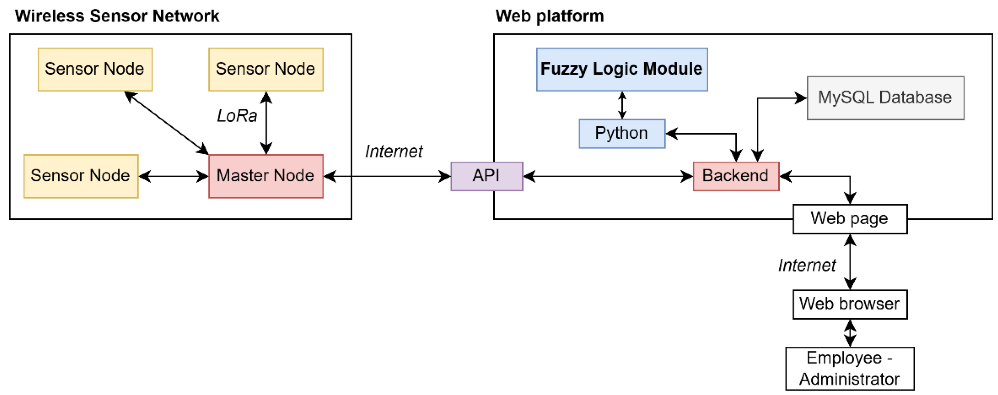
Figure 2.
Block diagram of the Sensor Node’s components.
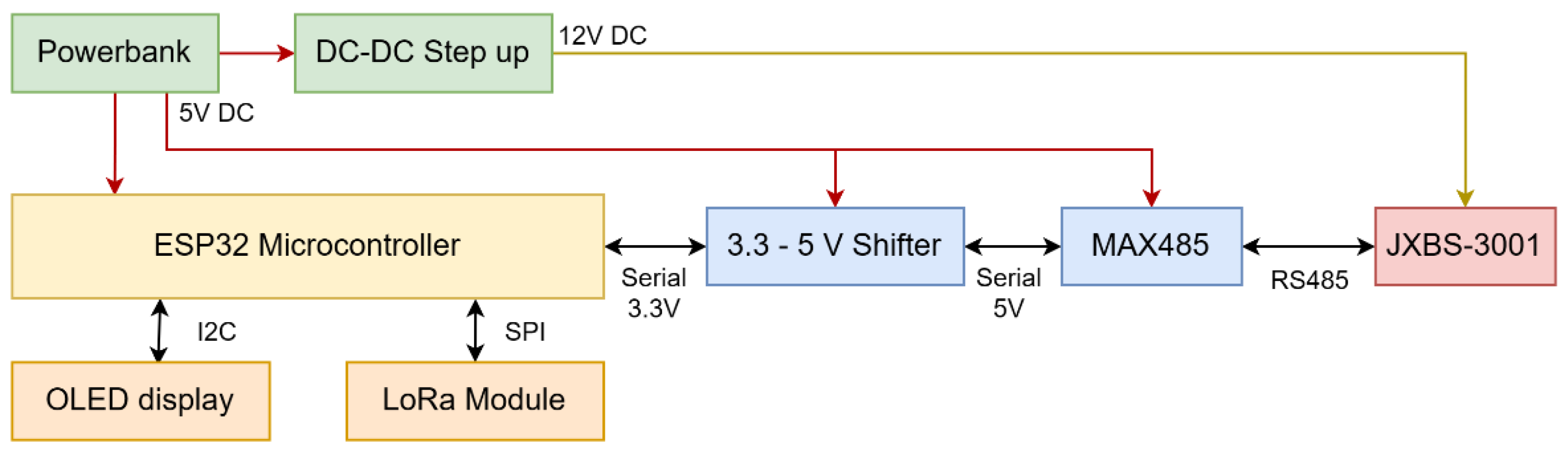
Figure 3.
Node distribution on Rancho Tajeli.
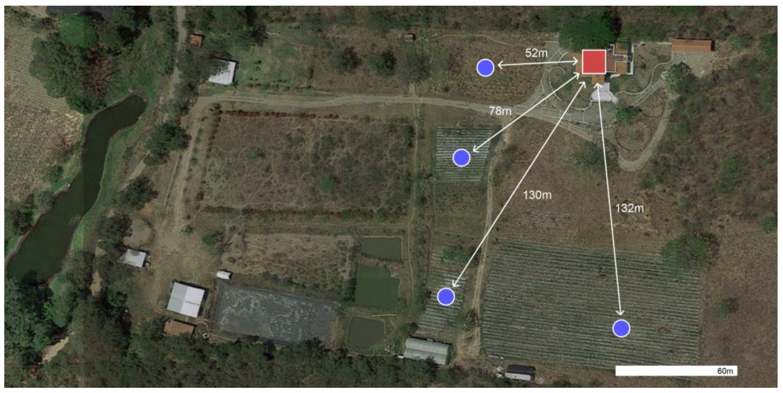
Figure 4.
Implementation of a sensor node on a stevia Morita II crop.
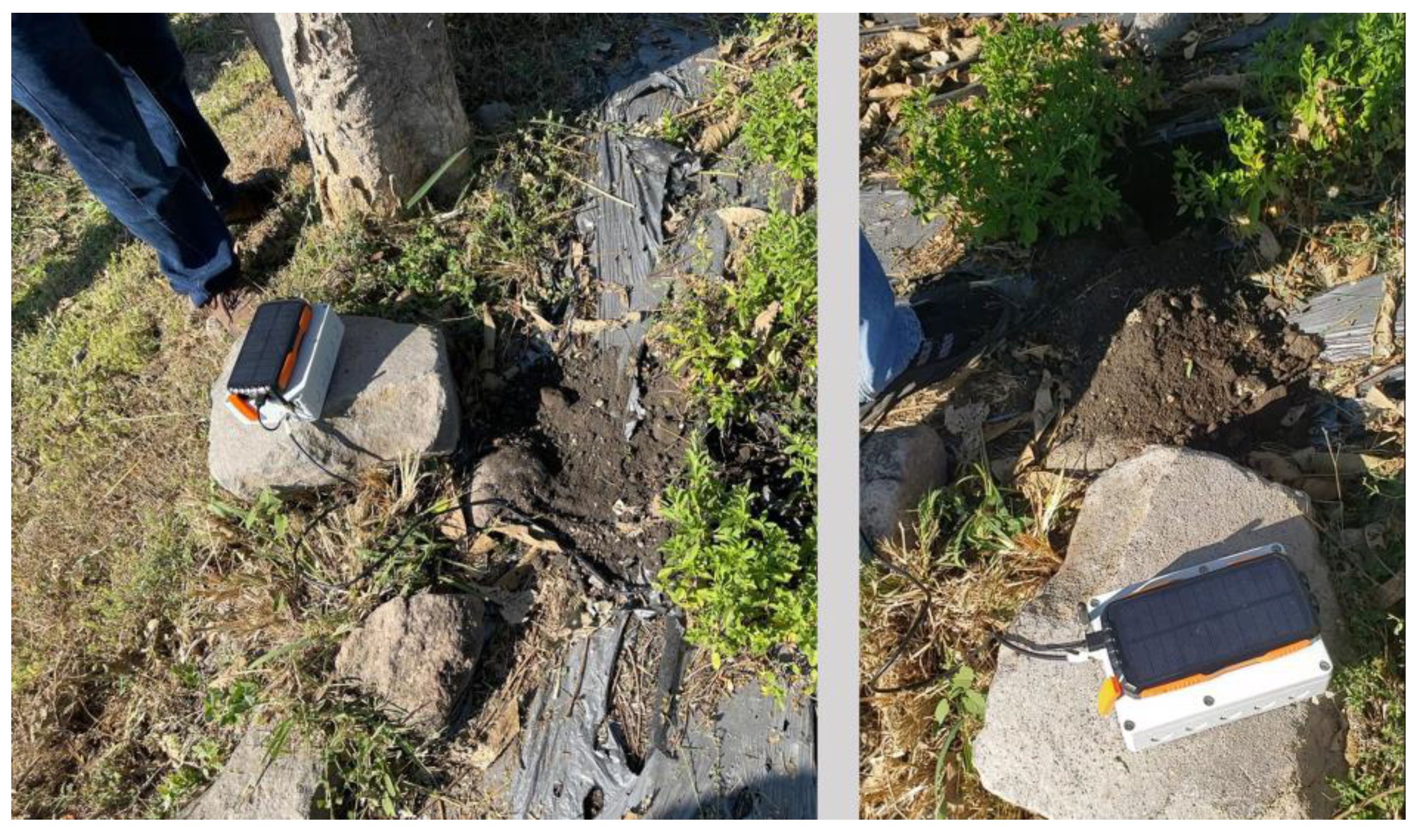
Figure 5.
Web platform structure.

Figure 6.
Expected JSON for the API’s endpoint for adding measurements, it supports different node types and showcases different node addresses.
Figure 6.
Expected JSON for the API’s endpoint for adding measurements, it supports different node types and showcases different node addresses.
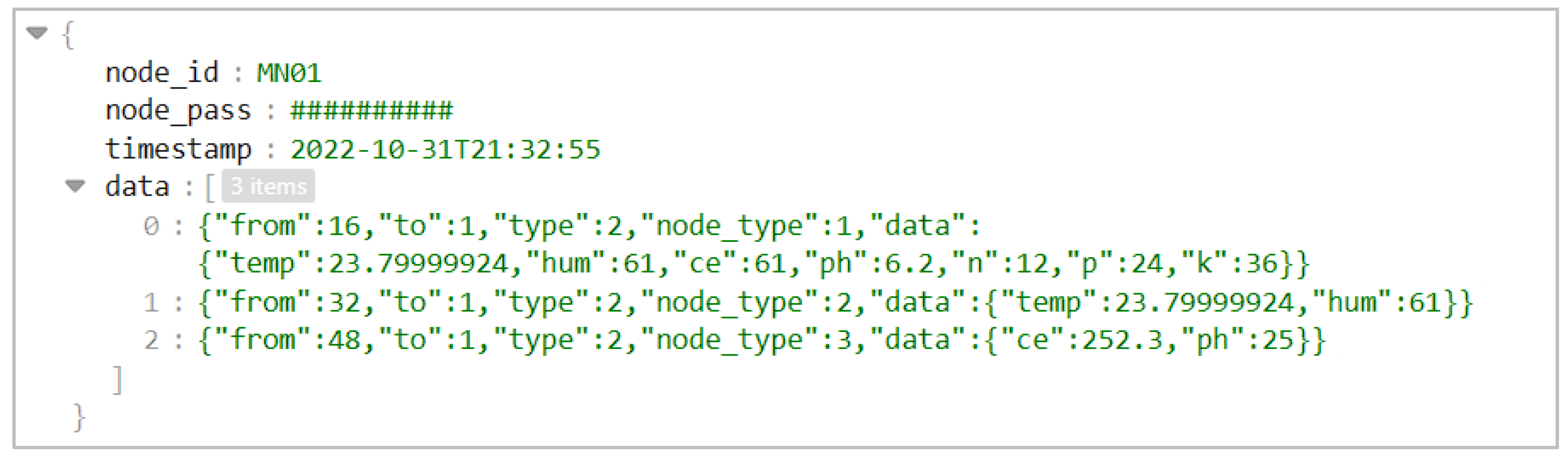
Figure 7.
FLM composed of three interconnected Fuzzy Models that determine Physicochemical Quality, Macronutrient Concentration and Soil Quality.
Figure 7.
FLM composed of three interconnected Fuzzy Models that determine Physicochemical Quality, Macronutrient Concentration and Soil Quality.
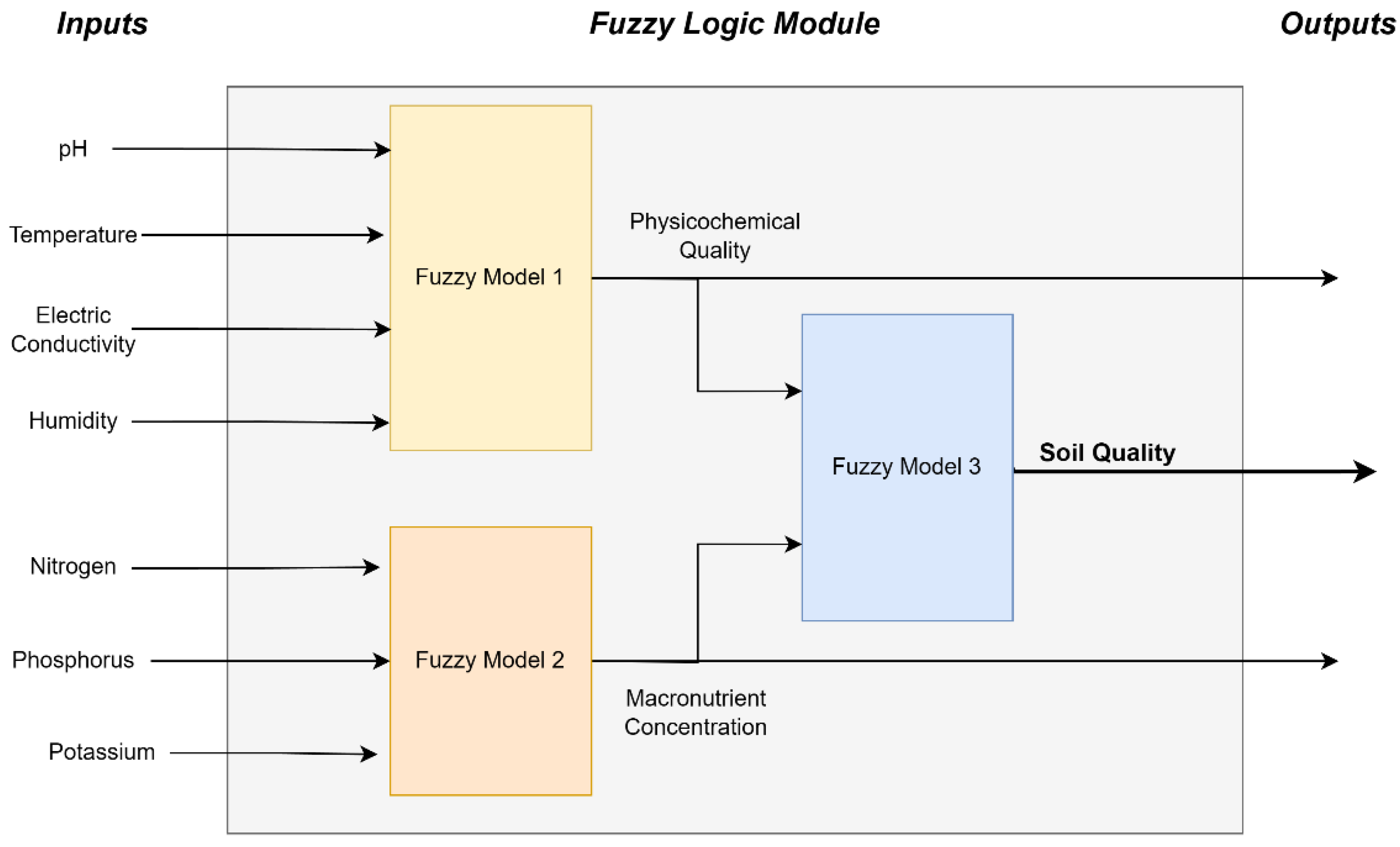
Figure 8.
Visual representation of each linguistic term of (a) Input pH MFs; (b) Input Temperature’s MFs.
Figure 8.
Visual representation of each linguistic term of (a) Input pH MFs; (b) Input Temperature’s MFs.
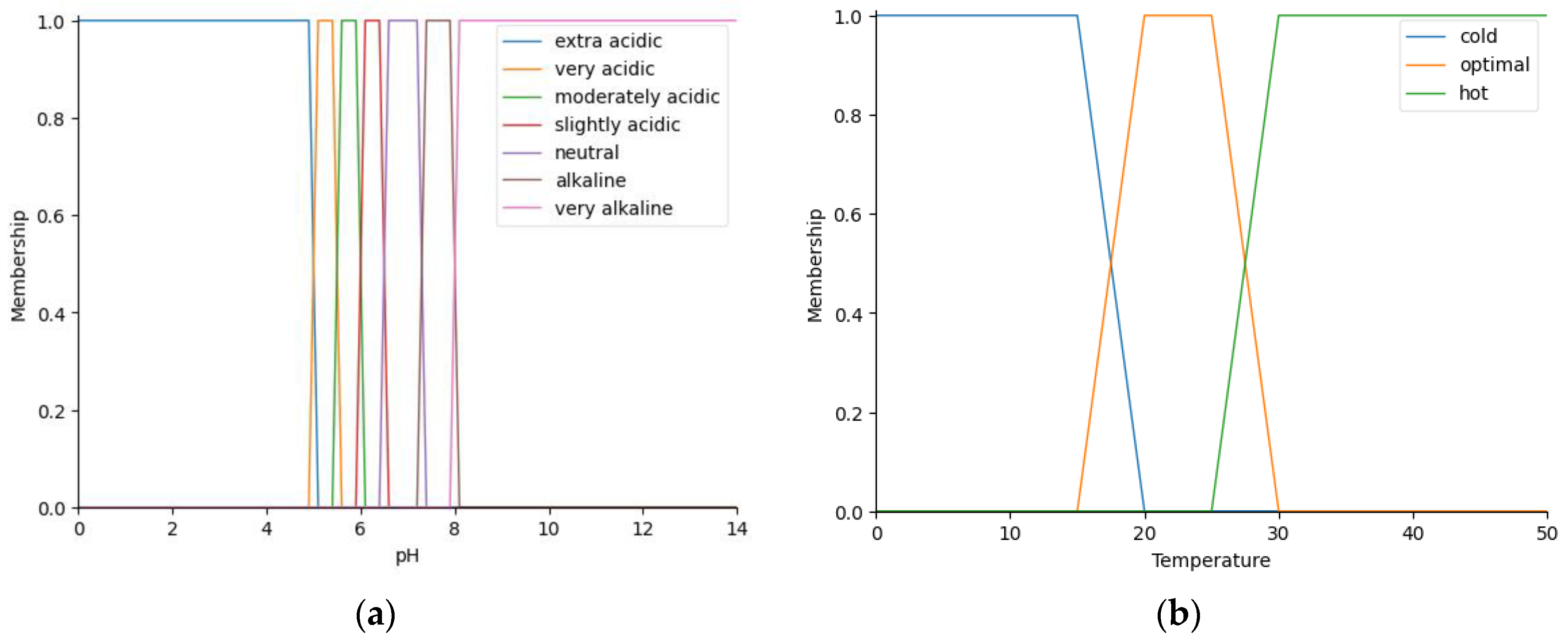
Figure 9.
Visual representation of each linguistic terms of (a) Soil Quality MFs; (b) Macronutrient Concentration MFs.
Figure 9.
Visual representation of each linguistic terms of (a) Soil Quality MFs; (b) Macronutrient Concentration MFs.
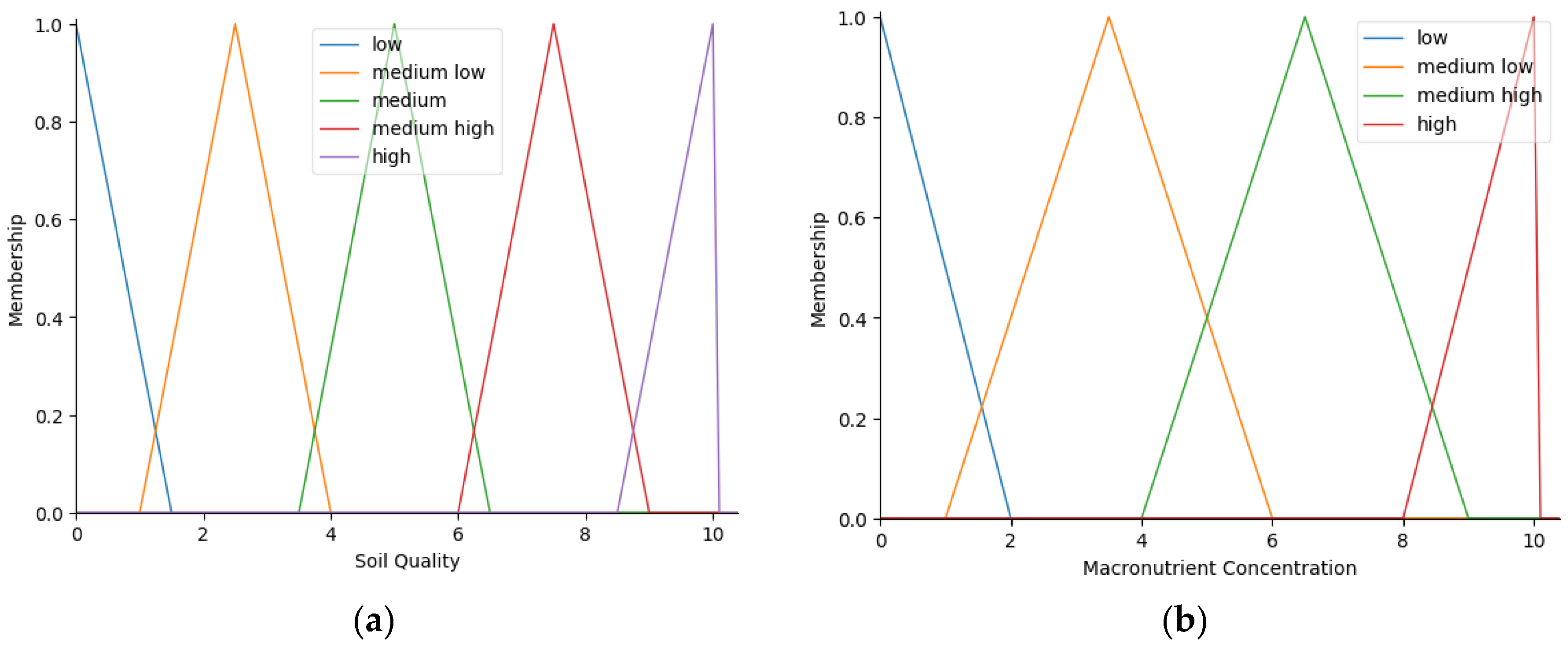
Figure 10.
(a) Main menu of the web platform. (b) Historical data section, it includes a plot showing all parameters.
Figure 10.
(a) Main menu of the web platform. (b) Historical data section, it includes a plot showing all parameters.
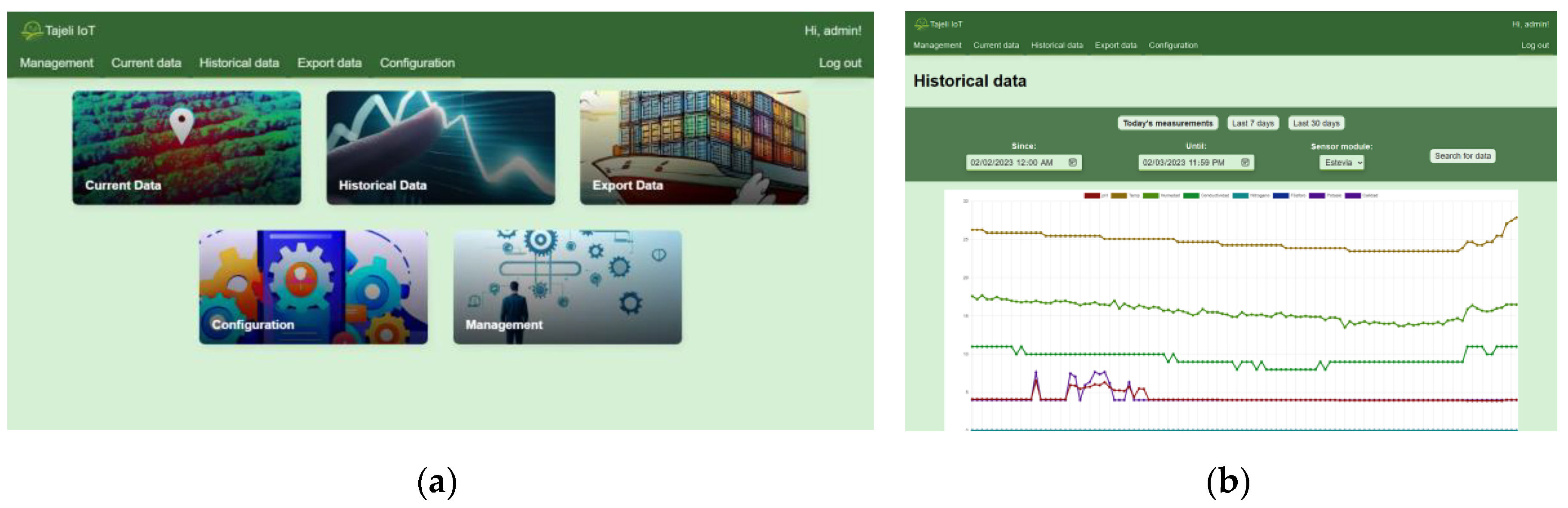
Figure 11.
(a) Export data section of the web platform, it shows the query menu that allows for date range selection and node selection. (b) CSV file downloaded using the data export section of the web platform.
Figure 11.
(a) Export data section of the web platform, it shows the query menu that allows for date range selection and node selection. (b) CSV file downloaded using the data export section of the web platform.
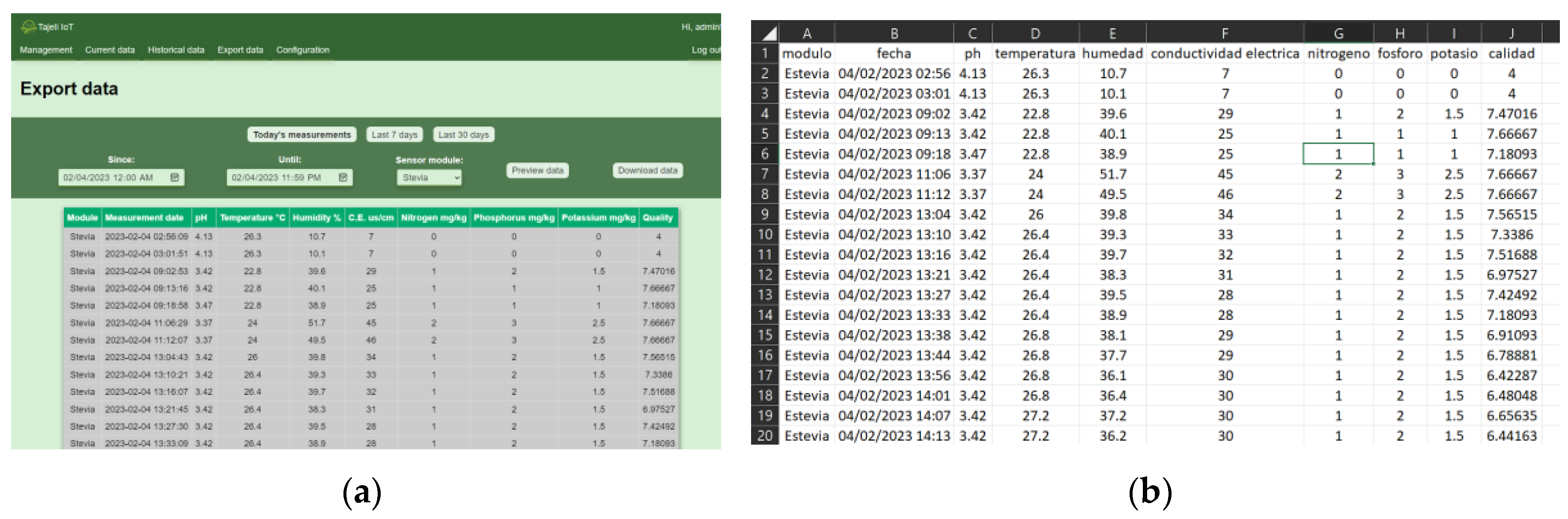
Figure 12.
Monitored variables evolution over one day, plot generated using the web platform.
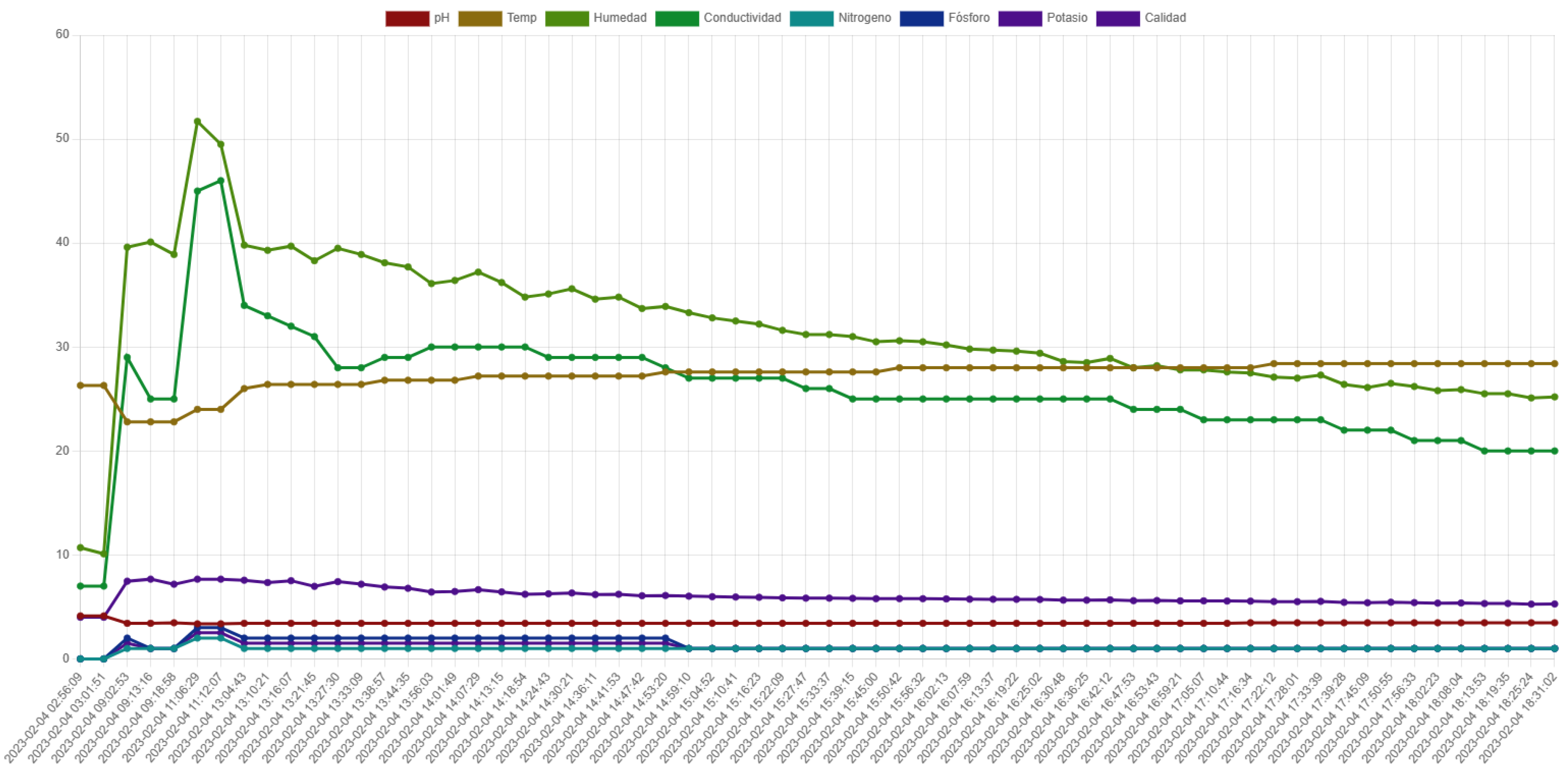
Figure 13.
Histograms of data collected using the monitoring system.
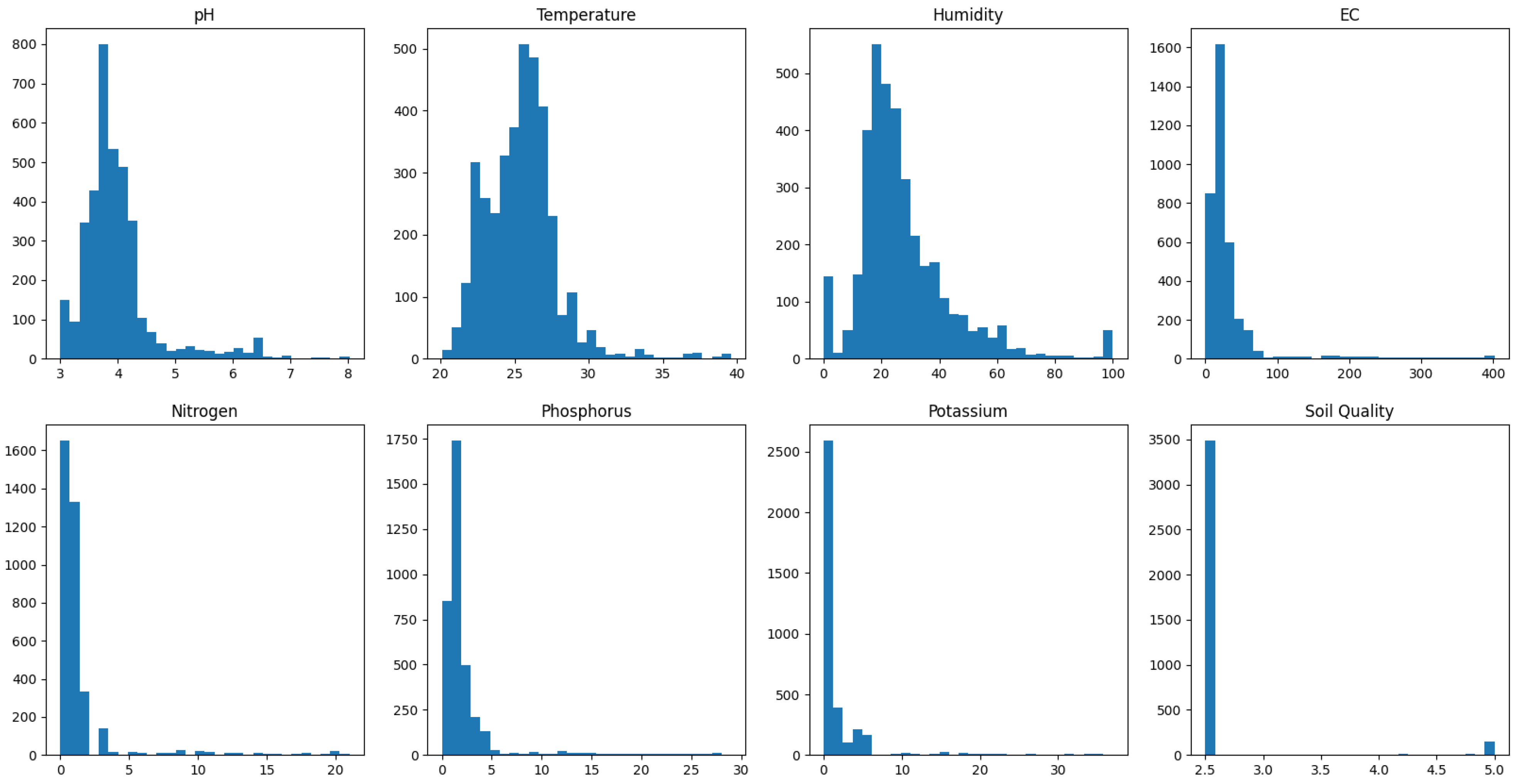
Figure 14.
(a) Scatter plot of the fuzzy model compared to the linear regression model using collected data from stevia crop. (b) Scatter plot of the fuzzy model compared to the linear regression model using random generated data.
Figure 14.
(a) Scatter plot of the fuzzy model compared to the linear regression model using collected data from stevia crop. (b) Scatter plot of the fuzzy model compared to the linear regression model using random generated data.
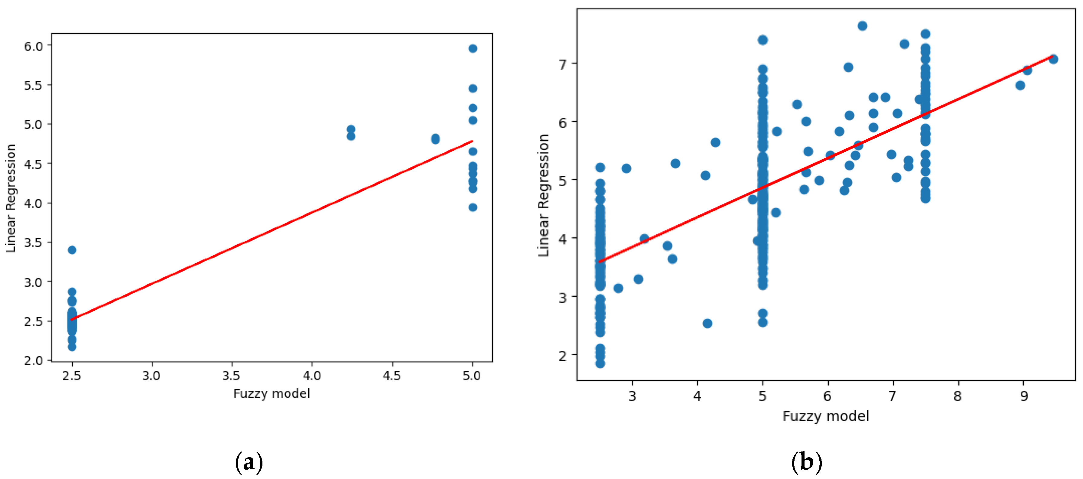
Figure 15.
Histograms of the random generated data for fuzzy model validation.
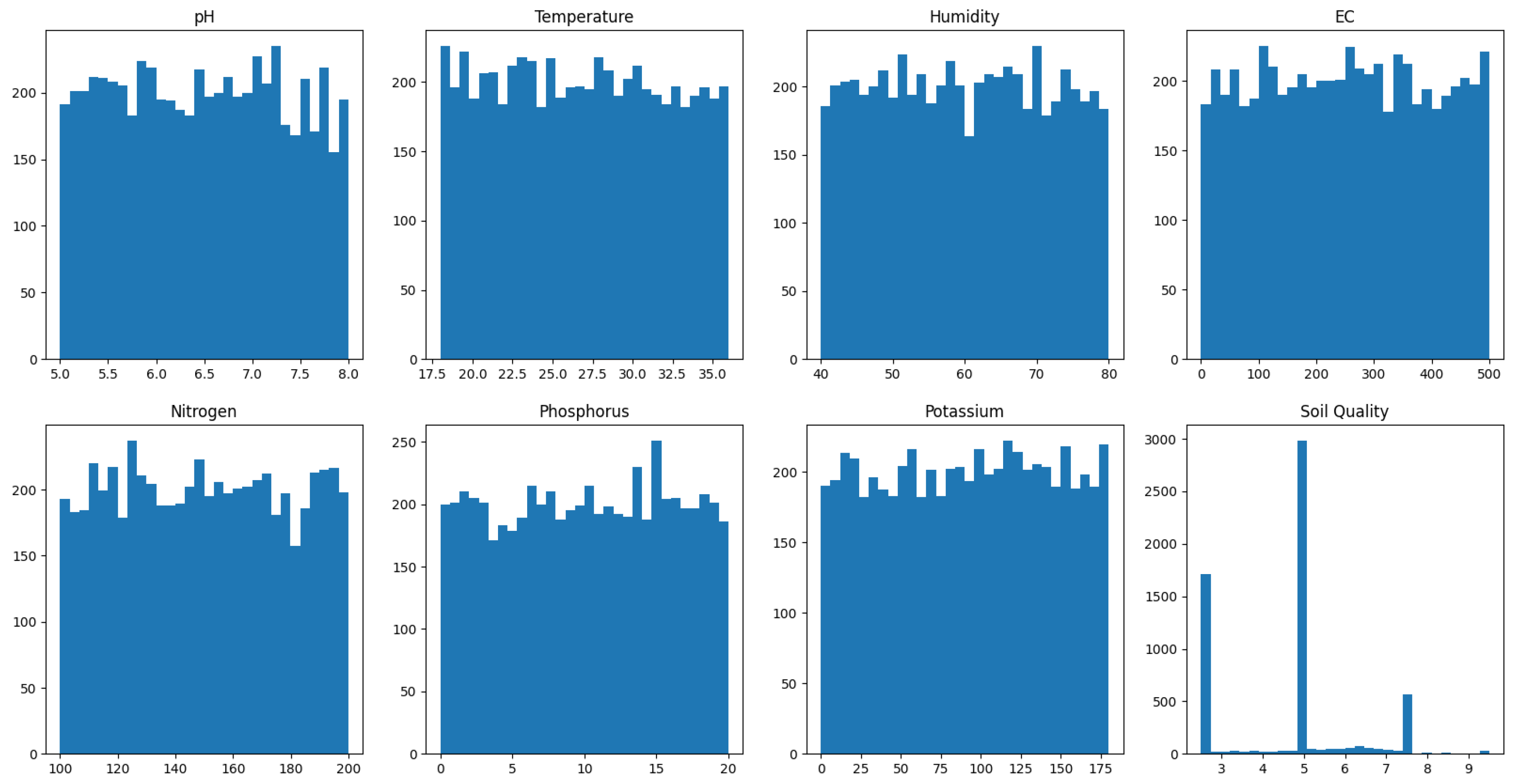
Table 1.
Fuzzy Model Inputs.
| Soil parameter | Universe of Disclosure | Linguistic term | Parameter unit | MF type | MF Parameters | |||
|---|---|---|---|---|---|---|---|---|
| a | b | c | d | |||||
| pH | extra acidic | - | Trapezoidal | 0 | 0 | 4.9 | 5.1 | |
| very acidic | Trapezoidal | 4.9 | 5.1 | 5.4 | 5.6 | |||
| moderately acidic | Trapezoidal | 5.4 | 5.6 | 5.9 | 6.1 | |||
| 0 - 14 | slightly acidic | Trapezoidal | 5.9 | 6.1 | 6.4 | 6.6 | ||
| neutral | Trapezoidal | 6.4 | 6.6 | 7.2 | 7.4 | |||
| alkaline | Trapezoidal | 7.2 | 7.4 | 7.9 | 8.1 | |||
| very alkaline | Trapezoidal | 7.9 | 8.1 | 14 | 14 | |||
| Temperature | cold | °C | Trapezoidal | 0 | 0 | 15 | 20 | |
| 0 - 50 | optimal | Trapezoidal | 15 | 20 | 25 | 30 | ||
| hot | Trapezoidal | 25 | 30 | 50 | 50 | |||
| Humidity | dry | % | Trapezoidal | 0 | 0 | 65 | 75 | |
| 0 - 100 | optimal | Trapezoidal | 65 | 75 | 85 | 95 | ||
| wet | Trapezoidal | 85 | 95 | 100 | 100 | |||
| Electric Conductivity | low | uS/cm | Trapezoidal | 0 | 0 | 450 | 550 | |
| 0 - 1500 | medium | Trapezoidal | 450 | 550 | 950 | 1050 | ||
| high | Trapezoidal | 950 | 1050 | 1500 | 1500 | |||
| Nitrogen | low | mg/kg | Trapezoidal | 0 | 0 | 106.6 | 126.6 | |
| 0 - 300 | medium | Trapezoidal | 106.6 | 126.6 | 177.5 | 197.5 | ||
| high | Trapezoidal | 177.5 | 197.5 | 300 | 300 | |||
| Phosphorus | low | mg/kg | Trapezoidal | 0 | 0 | 4.2 | 4.8 | |
| 0 - 20 | medium | Trapezoidal | 4.2 | 4.8 | 8.8 | 9.4 | ||
| high | Trapezoidal | 8.8 | 9.4 | 20 | 20 | |||
| Potassium | low | mg/kg | Trapezoidal | 0 | 0 | 44.1 | 54.1 | |
| 0 - 180 | medium | Trapezoidal | 44.1 | 54.1 | 111.6 | 121.6 | ||
| high | Trapezoidal | 111.6 | 121.6 | 180 | 180 | |||
Table 2.
Fuzzy Model Outputs.
| Output name | Universe of Disclosure | Linguistic term | MF type | MF Parameters | ||
|---|---|---|---|---|---|---|
| a | b | c | ||||
| Soil Quality | low | Triangular | 0 | 0 | 1.5 | |
| medium low | Triangular | 1 | 2.5 | 4 | ||
| 0 – 10 | medium | Triangular | 3.5 | 5 | 6.5 | |
| medium high | Triangular | 6 | 7.5 | 9 | ||
| high | Triangular | 8.5 | 10 | 10 | ||
| Macronutrient Concentration | low | Triangular | 0 | 0 | 2 | |
| 0 – 10 | medium low | Triangular | 1 | 3.5 | 6 | |
| medium high | Triangular | 4 | 6.5 | 9 | ||
| high | Triangular | 8 | 10 | 10 | ||
| Physicochemical Quality | low | Triangular | 0 | 0 | 1.5 | |
| medium low | Triangular | 1 | 2.5 | 4 | ||
| 0 -10 | medium | Triangular | 3.5 | 5 | 6.5 | |
| medium high | Triangular | 6 | 7.5 | 9 | ||
| high | Triangular | 8.5 | 10 | 10 | ||
Table 3.
Fuzzy Model Rule list for Macronutrient Concentration.
| Nitrogen | Phosphorus | Potassium | Output’s activated MF | Corresponding output |
|---|---|---|---|---|
| 0 | 0 | 0 | low | Macronutrient Concentration |
| 0 | 0 | 1 | medium low | |
| 0 | 1 | 0 | medium low | |
| 1 | 0 | 0 | medium low | |
| 0 | 1 | 1 | medium high | |
| 1 | 0 | 1 | medium high | |
| 1 | 1 | 0 | medium high | |
| 1 | 1 | 1 | high |
Disclaimer/Publisher’s Note: The statements, opinions and data contained in all publications are solely those of the individual author(s) and contributor(s) and not of MDPI and/or the editor(s). MDPI and/or the editor(s) disclaim responsibility for any injury to people or property resulting from any ideas, methods, instructions or products referred to in the content. |
© 2023 by the authors. Licensee MDPI, Basel, Switzerland. This article is an open access article distributed under the terms and conditions of the Creative Commons Attribution (CC BY) license (http://creativecommons.org/licenses/by/4.0/).
Copyright: This open access article is published under a Creative Commons CC BY 4.0 license, which permit the free download, distribution, and reuse, provided that the author and preprint are cited in any reuse.


