
Submitted:
10 March 2025
Posted:
11 March 2025
You are already at the latest version
Abstract
With the ongoing development of Intelligent Transportation Systems (ITS), traffic flow prediction methods have become a cornerstone of its technology. Accurate traffic flow forecasting can significantly support traffic management and decision-making.However, the expanding demand for such systems presents new challenges for the development of traffic flow prediction technologies. This paper offers a comprehensive review of traffic flow prediction methods utilized in ITS, classifying them into three categories: statistical-based, machine learning-based, and deep learning-based methods. By analyzing the principles, advantages, limitations, and applications of each approach within ITS, and comparing them through practical case studies, the paper emphasizes the pivotal role of deep learning models in improving prediction accuracy, particularly in short-term traffic forecasting. Despite the notable success of deep learning methods in short-term predictions, challenges persist, such as model generalization across diverse traffic scenarios and difficulties in long-term traffic flow forecasting. The paper concludes by suggesting future research directions, aiming to provide new perspectives and enhance the development of ITS technologies.
Keywords:
intelligent transportation systems
; statistical analysis theory
; machine learning
; deep learning
1. Introduction
1.1. Theme Background and Significance
In modern society, road traffic holds significant importance in both the economy and daily life. However, with the rapid development of the automotive industry, there is a lack of sufficient awareness regarding the limitations and scarcity of traffic resources. The surge in travel demand has placed immense pressure on transportation systems. Although the construction of new roads can alleviate congestion, most cities have turned to advanced technologies due to limitations in urban space and costs. In recent years, many countries worldwide have invested substantial resources into the research and development of intelligent transportation systems (ITS), which have played a critical role in alleviating congestion and enhancing traffic flow efficiency.
As a key component of smart cities, ITS plays a vital role in improving environmental quality and enhancing the quality of life for residents. ITS utilizes real-time monitoring, intelligent traffic signal control, and other technological means to directly reduce traffic congestion, lower accident rates, and relieve urban traffic pressures. Additionally, ITS can decrease vehicle idling, thereby reducing exhaust emissions and indirectly improving urban environmental quality. Most importantly, through services such as intelligent navigation systems and real-time public transportation information, ITS enhances the convenience and comfort of residents’ travel [1,2].
In summary, ITS plays an irreplaceable role in achieving the development goals of smart cities. However, ITS is a complex management system, encompassing multiple subsystems such as rail transit management, intelligent traffic signal management, and vehicle navigation. To ensure the efficient operation of the ITS, traffic flow prediction technology is of paramount importance.
Traffic forecasting technology is the cornerstone of intelligent transportation systems. Its core principle is to model urban road networks, highways, and rail transit systems, and, by integrating historical traffic data, predict traffic conditions for specific future time periods. By accurately predicting traffic flow data, traffic management authorities can more effectively guide vehicles, mitigate urban traffic congestion, and improve vehicle throughput efficiency. Accurate traffic flow forecasting also helps to schedule vehicle operations in rail systems, preventing public safety issues that may arise from large crowds gathering for extended periods, thus ensuring the safety of citizens’ travel. Furthermore, precise traffic forecasting can reduce the energy consumption associated with travel, contributing to the construction of low-carbon and environmentally friendly cities. Therefore, further enhancement of traffic flow forecasting technologies is imperative.
1.2. Research Status
The core of traffic flow prediction tasks lies in analyzing historical data to forecast future traffic flow trends, thus providing decision-making support to traffic management authorities. This requires a substantial amount of data, much of which is collected through sensors, cameras, and other monitoring technologies, and exhibits both temporal and spatial dependencies. Temporal dependency is mainly reflected in patterns such as the similarity in peak travel times during weekday rush hours and holidays. Spatial dependency is manifested in how the current traffic situation is influenced by the historical traffic conditions of upstream, downstream, and adjacent road monitoring points. Additionally, traffic flow is also affected by external factors such as weather conditions, holidays, and the distribution of points of interest, all of which significantly impact the accuracy of traffic flow predictions [3]. The related data is highly nonlinear and complex, making it difficult for traditional statistical and machine learning methods to accurately capture and model.
In recent years, the development of deep learning technologies has introduced powerful capabilities in feature extraction and pattern recognition, showing great potential in the field of traffic forecasting. Deep learning models such as deep neural networks, recurrent neural networks, and long short-term memory networks are capable of processing complex spatiotemporal data, leading to significant improvements over traditional methods. Moreover, the adaptive ability of deep learning allows it to maintain prediction accuracy even when faced with substantial noise and multidimensional features in traffic data.
Academia both domestically and internationally has conducted extensive and in-depth research in the field of traffic forecasting, developing a range of methods tailored to different application scenarios. These include traffic flow prediction for multi-intersection systems [4], highway traffic volume forecasting [5], and urban road traffic flow prediction [6], among others. Commonly used techniques include statistical analysis methods, machine learning approaches, and deep learning methods, which will be discussed in detail in the main body of this paper.
1.3. The Purpose of This Study
In future developments, smart cities will emerge as the predominant trend in urban growth. With the continuous advancement and application of technology, smart cities will play an increasingly significant role in urban management, social governance, and economic development. As a critical component of smart cities, the development level of intelligent transportation systems (ITS) will directly impact urban traffic conditions and residents’ quality of life. The primary objective of this research is to promote innovation and development in traffic flow prediction technologies while providing scientific and reliable decision-making support for urban traffic management. By integrating state-of-the-art data processing techniques and machine learning algorithms, this study will analyze the advantages and disadvantages of various technologies, exploring the challenges they present and their future development trajectories. This research is anticipated to provide more precise data support for key areas such as urban traffic planning, traffic signal control, and emergency response, thereby effectively mitigating traffic congestion, enhancing public transportation efficiency, and ensuring traffic safety. Furthermore, this study will offer novel research perspectives to related fields such as transportation science, computer science, and data analysis.
1.4. Brief Layout of the Paper
The structure of this paper is clear and straightforward. To provide readers with a better understanding of the importance of traffic flow prediction in smart cities and the specific implementation methods of such predictions, this paper first elaborates on the significance of traffic forecasting systems within the context of smart cities. This includes, but is not limited to, mitigating traffic congestion, reducing accident rates, improving urban environmental quality, and enhancing residents’ quality of life. Next, the paper outlines the implementation methods for traffic flow prediction, starting with earlier prediction approaches based on statistical analysis theories and progressing to the latest applications of deep learning methods. A summary of the data sets required for related simulations is also provided. The paper then presents a comparative analysis of methods from different eras through case studies to highlight the most effective approach at present. Finally, the paper concludes by summarizing the advantages and disadvantages of all the methods discussed, offering forward-looking perspectives for the future development of traffic flow prediction.
2. Prediction Method Based on Statistical Analysis Theory
2.1. Introduction
Traditional statistical methods have been in use for an extended period in traffic flow prediction, particularly in the early stages of intelligent transportation system development. While deep learning and machine learning techniques have gradually gained prominence in recent years, traditional statistical methods still hold significant value in short-term traffic forecasting or scenarios with limited data. These methods are widely adopted for short-term traffic prediction due to their relatively simple theoretical foundation, lower computational complexity, and stable prediction results. The essence of traditional statistical methods lies in constructing mathematical models based on historical traffic data to capture characteristic patterns from time series, thereby enabling the prediction of future traffic flow.
2.2. Specific Methods Listed
- (1)
- Historical average model (HA)
The historical average method is a basic forecasting technique commonly employed to predict data with periodic or seasonal patterns. It forecasts future values by computing the average of the same time period from historical data, assuming that the data follows a certain cyclical pattern. The method is simple, and its parameters can be estimated online using the least squares (LS) method. It is capable of handling variations in traffic flow over different times and periods to some extent. However, its static prediction performance is limited, as it does not reflect the inherent uncertainty and nonlinear characteristics of dynamic traffic flow. In particular, it is unable to address the impact of random disturbances or respond to unforeseen events, such as accidents, within the traffic system [7].
- (2)
- Autoregressive Integrated Moving Average model (ARIMA)
Unlike other time series methods that require fixed initialization for simulation, the ARIMA model is composed of three components: Autoregression (AR), Differencing (I), and Moving Average (MA). By fitting the historical data, the model generates parameters and makes predictions. It views traffic flow at a given time as a more general non-stationary stochastic process, typically with three or six model parameters [8].
Based on a substantial amount of continuous data, the ARIMA model offers high prediction accuracy, making it particularly suitable for stable traffic flows. However, the model primarily approaches prediction from a pure time series analysis perspective and does not account for the flow relationships between upstream and downstream road sections. Therefore, it is recommended to use this model in conjunction with other models for more comprehensive predictions [9].
- (3)
- Kalman filter model
Kalman filtering theory (KF), introduced by Kalman in 1960, has found applications in various domains, including time series modeling in statistics and economics. Kalman filtering is typically employed in non-stationary stochastic environments and offers relatively low computational complexity. However, it is only applicable to linear systems and is highly sensitive to noise. For state estimation and prediction in nonlinear systems, the use of extended Kalman filtering or nonlinear filtering methods is necessary. Given that the model is based on linear estimation, its performance may deteriorate when the prediction interval is less than 5 minutes and when the randomness and non-linearity of traffic flow variations are more significant [10].
2.3. Disadvantages
Although prediction methods based on statistical analysis theory have demonstrated good performance on small datasets with short observation periods and limited time series, the predictive capability of these statistical models is limited in traffic forecasting applications. This is due to their simple and transparent computational structure, their exclusive focus on time series data, and their lack of consideration for the complexity of spatiotemporal relationships. To address this challenge, some studies have developed extended time series methods, such as ST-ARIMA [11] and VARMA [12], which incorporate the interaction between space and time in a novel manner. However, because these methods rely on explicit parameterized functions with strong assumptions during the modeling process, they are not well-suited for simulating real-world traffic scenarios。
3. Traditional Machine Learning Models
3.1. Introduction
In recent years, machine learning methods have made significant strides in various fields such as industrial control, finance, and healthcare. This tool has also proven highly effective in the transportation domain, particularly in the development and application of Intelligent Transportation Systems (ITS). In the context of traffic flow prediction, machine learning methods, compared to traditional statistical techniques, are better able to adapt to the evolving nature of traffic networks. Through the use of historical data, pattern recognition, and the establishment of dynamic nonlinear models, machine learning methods play a vital role in enabling precise traffic flow predictions.
3.2. Specific Methods
Traditional machine learning methods applied in traffic prediction can be broadly categorized into three types: feature extraction-based methods, Gaussian process modeling methods, and state space modeling methods [13].
- (1)
- Feature extraction-based methods are primarily employed to train regression models to solve practical traffic prediction problems. Their main advantage lies in their simplicity and ease of implementation. However, these methods also suffer from limitations, such as focusing only on time series data and neglecting the complexities of spatiotemporal relationships. Cheng et al. [14] proposed an adaptive K-Nearest Neighbors (KNN) algorithm that treats spatial features of the road network as adaptive spatial neighbor nodes, time intervals, and spatiotemporal iso value functions. The algorithm was evaluated using speed data collected from highways in California and urban roads in Beijing.
- (2)
- Gaussian process methods utilize multiple kernel functions to capture the internal features of traffic data, while considering both spatial and temporal correlations. These methods are useful and practical for traffic forecasting but come with higher computational complexity and greater data storage demands when compared to feature extraction-based methods.
- (3)
- State space modeling methods assume that the observations are derived from a hidden Markov model, which is adept at capturing hidden data structures and can naturally model uncertainty within the system. This is an ideal characteristic for traffic flow prediction applications. However, these models can be challenging when it comes to establishing nonlinear relationships. Therefore, they are not always the best choice for modeling complex dynamic traffic data, particularly in long-term forecasting scenarios. Tu et al. [15] introduced a congestion pattern prediction model, SG-CNN, based on a hidden Markov model and compared it with the well-known ARIMA baseline model for traffic prediction. Experimental results demonstrated that the SG-CNN model exhibited strong performance.
4. Deep Learning Models
4.1. Introduction
Deep learning technology, an extension of machine learning, is comprised of numerous processing layers, which enable the learning of features at high levels of abstraction. In recent years, various sensor devices have been utilized to capture urban traffic parameters, generating large volumes of data with diverse types and characteristics. At the same time, deep learning techniques have demonstrated their capacity for high-dimensional data mining, extracting complex spatiotemporal dependencies from intricate traffic datasets, thus improving the accuracy of traffic predictions.
Essentially, deep learning bypasses the need for human involvement in the feature selection process. As a widely researched area in recent years, deep learning has achieved notable success in fields such as image recognition, object detection, and natural language processing. Compared to traditional machine learning, deep learning offers a broader range of applications, significantly expanding the field of artificial intelligence. The core of deep learning lies in constructing machine learning models with multiple hidden layers, which are trained on vast amounts of data to derive more meaningful features, thereby enhancing the accuracy of prediction and classification tasks. Prominent and effective deep learning models currently include Convolutional Neural Networks (CNN), Autoencoders, Recurrent Neural Networks (RNN), Graph Convolutional Networks (GCN), Attention Mechanisms with Transformers, and Hybrid Neural Networks in deep learning.
4.2. Multi-Layer Perceptron Network (MLP)
Among the many deep neural networks, the MLP was among the first to be applied in short-term traffic flow forecasting. The MLP is the simplest type of deep neural network, and a typical MLP consists of an input layer, hidden layers, an output layer, and nonlinear activation functions, forming a multi-layer feedforward artificial neural network, as shown in Figure 1. In the MLP, the input layer receives the input data and performs feature normalization, while the hidden layers process the input signals. The output layer makes decisions or predictions based on the processed information. Figure 1 illustrates a single-neuron perceptron model, where the activation function φ (Equation (1)) is a nonlinear function that maps the summation function (xw + b) to the output value y. In Equation (1), the terms x, w, b, and y represent the input vector, the weighted vector, the bias, and the output value, respectively [16]. Figure 2 shows the structure of the MLP model.
y=φ(xw+b),
The Multi-Layer Perceptron (MLP) is capable of mapping multidimensional data to a one-dimensional output, solving the nonlinear issues that a single-layer network cannot address. MLP is trained using the Backpropagation (BP) algorithm, and by applying a simple MLP, high prediction accuracy can be achieved for short-term traffic flow forecasting. In the context of short-term traffic prediction, MLP is used to model the mapping relationship between the historical time series data (input) and the predicted results (output), enabling accurate traffic flow predictions. Slimania et al. [17] utilized MLP, SARIMA, and Support Vector Regression (SVR) algorithms to predict the traffic flow over a 42-day period on a road segment in Morocco, incorporating factors such as whether a given day is a holiday. Their experiment demonstrated that MLP outperformed the other two models in terms of prediction accuracy. Aljuaydi et al. [18] proposed a multivariate machine learning-based highway traffic flow prediction model for non-recurrent events, using a dataset that included five features: traffic flow, speed, density, road accidents, and rainfall, as well as two evaluation metrics, Root Mean Square Error (RMSE) and Mean Absolute Error (MAE). The MLP model used as a benchmark produced favorable forecasting results.
4.3. Convolutional Neural Networks (CNN)
Convolutional Neural Networks (CNN) are a class of deep learning models primarily used for processing and analyzing data with a grid-like structure, such as images and audio. The design inspiration for CNNs stems from the understanding of the animal visual system in biology. CNNs have achieved remarkable success in various domains, including image recognition, image classification, object detection, and semantic segmentation. A typical CNN consists of convolutional layers, pooling layers, and fully connected layers. In the convolutional layers, the network applies a series of filters to extract features from the input data, generating feature maps. The pooling layers serve to reduce the spatial dimensions of the feature maps, thereby decreasing computational complexity, often utilizing operations such as max pooling or average pooling. Finally, the fully connected layers map the high-level features to the final output, performing tasks such as classification or regression. These characteristics enable CNNs to effectively capture features of traffic data, thereby excelling in traffic flow prediction tasks. The corresponding structure is shown in Figure 3.
Fast R-CNN, introduced by Ross [19], incorporates multiple innovations to improve both training and testing speeds, while also enhancing detection accuracy. Bogaerts et al. [20] proposed a deep neural network using a CNN-LSTM architecture for multi-step prediction. The CNN-LSTM framework is capable of identifying spatial and temporal relationships within traffic data sourced from GPS trajectories. Moreover, they introduced a data reduction technique and compared it with the advanced TF algorithm, yielding improved prediction results.
4.4. Autoencoder (AE)
Autoencoders are an unsupervised neural network model that performs feature extraction by learning compressed representations of input data. An autoencoder (AE) works by training each layer of the network progressively, with each layer encoding and decoding the output of the previous layer. This process allows the model to gradually learn multi-level abstract features of the data. The objective of training each autoencoder layer is to minimize the reconstruction error, which is the difference between the input data and the reconstructed data [21]. The specific model structure is shown in Figure 4. Autoencoders have numerous variants, with sparse autoencoders being particularly effective at feature extraction. Sparse autoencoders can identify fewer but more meaningful features from the input data and can be combined with other deep learning techniques, such as Convolutional Neural Networks (CNNs) and Recurrent Neural Networks (RNNs), to further enhance performance. Sparse autoencoders are widely applied in the traffic domain.
4.5. Recurrent Neural Networks (RNN)
Recurrent Neural Networks (RNN) are deep learning architectures specifically designed to handle sequential data. Unlike traditional neural network models, RNNs possess the ability to maintain the continuous transmission of information across time steps, thereby enabling the retention of historical input data. Within its network structure, RNN employ a specific connection mechanism that ensures the output at each time step is influenced not only by the current input but also by the previous state. This characteristic significantly enhances the accuracy and robustness of the model in time-series predictions. The basic RNN model can be considered a time-series prediction tool with memory capabilities. In the field of traffic data analysis, where the data inherently contains complex spatiotemporal dependencies, RNNs and their various variants have been widely applied for traffic flow prediction [22].
RNN do not rigidly memorize fixed-length sequences; instead, they store information from previous time steps through their hidden states. A typical RNN structure is cyclical and consists of an input layer, an output layer, and a neural network unit. In this architecture, the RNN’s neural network unit not only establishes connections with the input and output layers but also possesses an internal loop that facilitates the flow of information across different time steps in the network. As shown in Figure 5, where xi represents the input at the i-th time step, and yi corresponds to the output generated by xi. The computation formula for the RNN model is as follows:
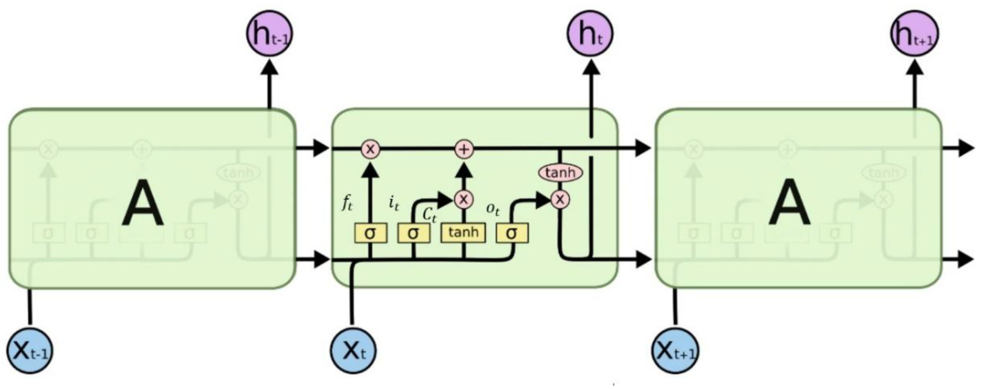
4.6. Long Short-Term Memory Recurrent Neural Networks (LSTM)
Due to the susceptibility of traditional RNNs to issues such as vanishing and exploding gradients, Long Short-Term Memory Recurrent Neural Networks (LSTM-RNNs) were developed to address these limitations. LSTM-RNNs introduce unique gating mechanisms and memory cells, which enable them to effectively capture long-term dependencies within sequential data. Compared to traditional RNNs, the invention of LSTM has paved new pathways for the development of RNN models. Particularly in the field of natural language processing, LSTMs have demonstrated superior performance over traditional RNNs, rapidly gaining widespread recognition and practical application.
The memory cell of an LSTM is primarily composed of the output gate, input gate, and forget gate.
The forget gate determines which information should be forgotten or retained from the cell state, and its computation is as follows:
The input gate consists of two components: a sigmoid layer that determines which values need to be updated, and a tanh layer that creates a new candidate value vector, which will be added to the cell state. The computation formula for the input gate is as follows:
The output gate determines the value of the hidden state, which contains key information about the observed sequence. The computation formula for the output gate is as follows:
Figure 6.
LSTM model diagram.
Traffic flow prediction based on RNNs has been widely applied. Zheng et al. [23] employed LSTM networks to predict traffic flow, analyzing the impact of various factors on the prediction performance of LSTMs. They further improved prediction accuracy by incorporating an attention mechanism-based Conv-LSTM module. Zhao et al. [24] proposed a traffic flow prediction model based on LSTM networks, integrating the temporal and spatial interactions of the road network. Unlike traditional prediction methods, the LSTM network considers the spatiotemporal dependencies of the traffic system through a two-dimensional network consisting of multiple memory units. Comparative experiments with other typical prediction models demonstrated that the proposed novel LSTM-based traffic prediction model delivers superior performance.
4.7. Gated Recurrent Unit (GRU)
In RNNs, the GRU is a variant that is simpler than the LSTM network while still effectively addressing long-term dependencies and the vanishing gradient problem. GRU retains key components of the gating mechanism, specifically the update gate and the reset gate, which regulate the flow of information. However, it omits the memory cell found in LSTM networks. Compared to LSTM, GRU has fewer parameters, resulting in improved computational efficiency. In many cases, it achieves comparable, or even superior, performance on various tasks. Its structural model is shown in Figure 7.
Update Gate: The purpose of the update gate is to determine the extent to which the hidden state at the current time step should retain information from the previous time step. The formula is as follows:
Reset Gate: The reset gate determines to what extent the hidden state from the previous time step should be disregarded. The formula is as follows:
Li et al. were the first to apply GRUs to traffic flow prediction and demonstrated through experiments that the GRU-based approach outperforms the ARIMA model in short-term traffic flow forecasting [25]. R. Dey et al. systematically evaluated three variants of the GRU in RNNs by preserving the structure and reducing the parameters in the update and reset gates. This approach achieved reduced computational costs while maintaining performance [26]. Chung et al. proposed a Gated Feedback RNN (GF-RNN) method, which extends the conventional approach of stacking multiple recurrent layers by introducing a gating mechanism. This method utilizes GRUs to address the vanishing gradient problem. By incorporating gating mechanisms between recurrent layers, each layer independently controls the flow and feedback of information, thereby enhancing the network’s ability to handle long-term dependencies and improving overall performance [27].
4.8. Graph Convolutional Neural Networks (GCN)
Since CNN is only applicable to modeling tasks of Euclidean data, and the nodes in a traffic network usually present an irregular graph structure, the Euclidean and non-Euclidean data structures are shown in Figure 8. Therefore, GCN [28], which models non-Euclidean space, gradually replaced CNN and became a research hotspot in the field of short-term traffic flow prediction [29].
Graph convolution operations can be broadly classified into two categories: spatial domain-based and spectral domain-based graph convolutions. Spatial domain methods define graph convolution as the aggregation of feature information between adjacent nodes in the graph. Spectral domain methods, on the other hand, begin by processing graph signals and introduce filters to derive graph convolution. This operation is interpreted as the process of removing noise from the graph signals. Both methods offer distinct advantages when handling graph data, and the appropriate approach can be selected based on the specific requirements of the task.
In most existing methods, Graph Convolutional Networks (GCNs) use a fixed adjacency matrix to model spatial dependencies in traffic networks. However, in real-world scenarios, spatial dependencies vary over time. Hu et al. proposed a Spatio-Temporal Graph Convolutional Network (GLSTGCN) for traffic prediction. They designed a graph learning module to capture dynamic spatial relationships in the traffic network and employed a gated mechanism with dilated causal convolution networks to capture long-term temporal correlations in traffic data. Experimental results demonstrate the superior performance of GLSTGCN [30].
To address the challenges of air traffic flow prediction, which involves complex spatial dependencies, nonlinear temporal dynamics, and weather influences, Li et al. proposed a Cross-Attention Diffusion Convolutional Recurrent Neural Network (CA-DCRNN). This model utilizes diffusion convolution to capture spatial dependencies and an encoder-decoder architecture with predefined sampling to handle temporal dependencies [31]. Zhao et al. combined GCN with GRU networks to capture spatiotemporal dependencies, and experimental results on two public datasets show that the GCN network exhibits strong spatial information capturing capability [32].
4.9. Attention Mechanism and Transformer
The attention mechanism is a technique that imitates the human visual or cognitive system and is widely used in the field of deep learning. It was initially widely used in the field of NLP [33] and later in fields such as computer vision. It assigns different weights to each element in the input sequence according to its importance. This weight is dynamically calculated based on the relevance between each element and the target.
Transformer is a deep learning framework primarily used for tasks such as natural language processing [34]. Different from the traditional CNN and RNN architectures, Transformer completely abandons these structures and is built on the attention mechanism. The model consists of Self-Attention and Feed-Forward Neural Networks, addressing the sequential computation limitations of RNNs, allowing for any two positions in the sequence to be treated equivalently, thereby overcoming the long-term dependency issue inherent in RNNs [35]. A diagram of the Transformer model is shown in Figure 9.
Yan et al. [36] utilized the multi-head attention mechanism and stacked layers to enable the Transformer to learn dynamic and hierarchical features in traffic data. They proposed the integration of global and local encoders to extract and fuse global and local spatial features, facilitating effective traffic flow prediction and providing a basis for traffic management strategies.
Fan et al. [37] introduced a novel Spatiotemporal Graph Sandwich Transformer (STGST) for traffic flow prediction. In STGST, two times Transformers equipped with temporal encoding and one spatial Transformer with structural and spatial encoding are designed to model long-range temporal and deep spatial dependencies, respectively. By structuring these two types of Transformers in a sandwich configuration, the model captures rich spatiotemporal interactions. Experimental studies demonstrate that STGST outperforms state-of-the-art baseline models.
4.10. Hybrid Neural Network
Standalone models often focus on extracting either temporal or spatial features. To model both spatial and temporal correlations in traffic data simultaneously, deep learning hybrid models integrate statistical analysis, machine learning, and deep learning techniques for spatiotemporal data processing. These hybrid models aim to overcome the limitations of single models, enhancing both the accuracy and robustness of traffic flow predictions. By combining various models and techniques, hybrid models can more comprehensively account for the spatiotemporal characteristics of traffic flow, providing stronger support for traffic management and planning. These hybrids primarily include categories such as CNN, RNN, LSTM, and GCN.
In recent years, the decomposition-reconstruction (DR) hybrid model has gained significant attention from researchers. Chen et al. classified DR-based models and thoroughly studied their applications in this field. A hybrid model based on DR for short-term traffic state prediction is shown in Figure 10 [38]. Guo et al. [39] proposed an attention mechanism-based Spatiotemporal Graph Convolutional Network (ASTGCN) model, which simultaneously models the three temporal attributes of traffic flow while using graph convolutional models and standard convolutions to extract spatial and temporal features. Furthermore, this model employs a spatiotemporal attention mechanism to effectively capture the dynamic spatiotemporal correlations in traffic data. Experimental results on the PEMS dataset show that the prediction performance of ASTGCN outperforms other baseline models.
5. Traffic Prediction Related Datasets
Data is extremely important for deep learning models. The quality of samples in the data set largely determines the prediction performance and generalization of the model. As shown in Table 1, this paper summarizes the commonly used, public, and real-world data sets in the field of short-term traffic flow prediction research and lists their basic characteristics.
5.1. Stationary Traffic Data
A fixed-traffic dataset refers to a collection of traffic state information, such as road traffic flow, speed, and lane occupancy, which is captured in real-time by stationary traffic data collection devices like cameras and lidar sensors. Since the data is collected using specialized equipment, it is generally more accurate and continuous.
- (1)
- PeMS: PeMS is a traffic flow database in California, which collects real-time data from more than 39,000 independent detectors on California highways. Among them, the detector data is mainly from highways and metropolitan areas. These data include information such as vehicle speed, flow, congestion, etc., which provide important basis for traffic management, planning and research. The minimum time interval of the data is 5 minutes, which is very suitable for short-term prediction. It enables the historical average method to automatically fill in the missing data. In the task of traffic flow prediction, the commonly used sub-datasets are PeMS03, PeMS04, PeMS07, PeMS08, PeMS-BAY, etc.
- (2)
- The METR-LA traffic dataset contains traffic information collected from detectors on freeway loops in Los Angeles County. The Los Angeles Freeway Dataset contains traffic data detected by 207 detectors from March 1 to June 30, 2012, with a sampling interval of 5 minutes.
- (3)
- The Loop dataset is mainly loop data in the Seattle area, covering data from four highways: I-5, I-405, I-90, and SR-520. The Loop dataset contains traffic status data from 323 sensor stations, with a sampling interval of 5 minutes [40].
- (4)
- The Korean urban area dataset UVDS contains data on major urban roads collected by 104 VDS sensors, with traffic characteristics such as traffic flow, vehicle type, traffic speed, and occupancy rate [41].
5.2. Mobile Traffic Data
As the demand for real-time and dynamic traffic information continues to increase, traditional fixed traffic data collection technologies and information processing methods, though relatively mature, face issues such as low coverage, high maintenance costs, and poor reliability. As a result, mobile traffic data collection technologies have gained significant attention. Common data collection methods include floating car data collection, drone-based collection, and crowdsourcing techniques. While such data requires processing, it is easier to obtain, highly accurate, and widely used in traffic flow prediction.
- (1)
- TaxiBJ Dataset: TaxiBJ is a dataset of Beijing taxi data, which includes trajectory and meteorological data from over 34,000 taxis in the Beijing area over a period of 3 years. The data is converted into inflow and outflow traffic for various regions. The sampling interval for the dataset is 30 minutes, and it is primarily used for traffic demand prediction.
- (2)
- Shanghai Taxi Dataset: This dataset, proposed by the Smart City Research Group at the Hong Kong University of Science and Technology, contains GPS reports from 4,000 taxis in Shanghai on February 20, 2007. The vehicle data is sampled at 1-minute intervals and includes information such as vehicle ID, timestamp, longitude and latitude, and speed.
- (3)
- SZ-taxi Dataset: The SZ-taxi dataset consists of taxi trajectory data from Shenzhen, covering the period from January 1 to January 31, 2015. The dataset focuses on the Luohu District of Shenzhen and includes data from 156 main roads. Traffic speeds for each road are calculated every 15 minutes in this dataset.
- (4)
- NYC Bike Dataset: The NYC Bike dataset records bicycle trajectories collected from the New York City Bike Share system. The dataset includes data from 13,000 bicycles and 800 docking stations, providing detailed information about bike usage and movement across the city.
5.3. Common Evaluation Indicators
Traffic flow prediction, as a typical regression problem, is commonly evaluated using performance metrics such as MAE, RMSE, and MAPE to assess the accuracy of the model’s predictions.
MAE (Mean Absolute Error): MAE is the average of the absolute differences between the observed and true values. It is the most intuitive method to represent the error by calculating the average absolute error between predicted and actual traffic flow values. Smaller MAE values indicate better model performance. The formula is as follows:
RMSE (Root Mean Square Error): RMSE is the square root of the mean of the squared differences between the observed and true values. By squaring the errors before averaging, larger deviations from the true values incur a greater penalty, making this metric sensitive to large errors. A smaller RMSE indicates better model performance. The formula is as follows:
MAPE (Mean Absolute Percentage Error): MAPE measures the relative error between the observed and true values as a percentage. The values range from 0 to 1 and reflect the accuracy of predictions in proportional terms. A smaller MAPE indicates better model performance. The formula is as follows:
6. Method Comparison and Analysis
In order to comprehensively evaluate the performance of different models in traffic flow prediction problems, this paper takes PEMS08 and METR-LA as examples and selects several commonly used models proposed in the field of traffic flow prediction. The specific situation is shown in the Table 2.
From the table, we can see that the traditional data-driven ARIMA model has unsatisfactory prediction results due to limited data mining. The prediction models LSTM and GRU based on deep learning have greatly improved the prediction accuracy. The prediction model based on hybrid neural network ASTGCN has the best overall prediction accuracy because it takes into account the temporal and spatial correlation. In general, compared with other traditional methods, deep learning has more accurate prediction results, faster calculation speed and can meet the requirements of high-precision real-time prediction, with obvious advantages. In data scenarios where algorithms such as Arima based on statistical methods are difficult to predict, the short-term traffic flow prediction method based on deep learning is still effective.
This paper summarizes the advantages and disadvantages of various traffic flow prediction methods, as shown in Table 3.
7. Conclusions and Future Perspectives
This paper reviews the main methods of traffic flow prediction in the construction of intelligent transportation systems. In the previous article, we introduced three major types of traffic flow prediction methods: statistics-based, machine learning-based, and deep learning-based methods. After discussing the principles, advantages, limitations, and applications of these methods in intelligent transportation systems, we found that with the rapid development of big data and artificial intelligence technologies, deep learning models have shown obvious advantages in traffic flow prediction, especially when dealing with large-scale, nonlinear, and high-dimensional data, their prediction accuracy and generalization ability are significantly better than traditional methods. These models play a vital role in the development of ITS, not only improving the efficiency and accuracy of traffic management, but also helping to optimize resource allocation, alleviate traffic congestion, and enhance the public’s travel experience.
Although the short-term traffic flow prediction method based on deep learning has obvious advantages over the other two methods, it also faces certain limitations and challenges. One of the main problems is data acquisition and processing. This paper finds that the data sets used in the current research are mainly from urban road traffic flow data. Therefore, the number of abnormal data samples in the training set is smaller than that of normal data, and the applicability to other types of areas (such as rural or suburban areas) still needs to be further verified. In addition, the generalization ability of the model in different traffic scenarios, especially in the context of extreme weather conditions, large-scale events or other special events, still needs to be improved. A potential solution is to expand the diversity and sources of datasets by merging different types of data (such as traffic flow, speed, travel time, density, weather, population and image data). The fusion of multimodal data can promote the improvement of model performance and expand its applicability [42].
In addition, with the continuous development of the field of traffic prediction, more and more traffic prediction models have been proposed. However, the field of traffic flow prediction lacks consistent experimental settings and standardized public datasets. Different scholars use different datasets in their research, and each dataset has various external factors, which complicates the ability to effectively compare the actual prediction performance. Establishing standardized experimental settings and public datasets will greatly accelerate the development of the field of traffic flow prediction and improve the comparability and repeatability of different studies.
At present, research on short-term and medium-term traffic flow prediction has made significant progress, while research on long-term traffic flow prediction is still relatively limited. Unlike short-term traffic flow prediction, long-term prediction usually lasts for months or even years. Long-term traffic flow prediction faces challenges such as unstable results, high data and model complexity, and complex spatiotemporal dependencies. How to further improve the accuracy of long-term traffic flow prediction models based on existing research is one of the important research directions in the future.
In summary, this study not only provides a new perspective and methodological contribution to the field of traffic flow prediction, but also points out the future research direction. With the continuous development of intelligent transportation systems and the increasing complexity of urban traffic management, traffic flow prediction technology will continue to play an important role. We look forward to more innovative research results in the future to jointly promote the development and application of traffic flow prediction technology.
Author Contributions
Conceptualization, R.L. and S.-Y.S.; methodology, R.L. and S.-Y.S.; writing—original draft preparation, R.L. and S.-Y.S.; supervision, S.-Y.S. All authors have read and agreed to the published version of the manuscript.
Funding
This research received no external funding.
Institutional Review Board Statement
Not applicable.
Informed Consent Statement
Not applicable.
Data Availability Statement
The data used to support the findings of this study are available from the corresponding author upon request.
Conflicts of Interest
The authors declare no conflicts of interest.
References
- Qingcai, C., Wei, Z., & Rong, Z. (2017, May). Smart city construction practices in BFSP. In 2017 29th Chinese Control And Decision Conference (CCDC) (pp. 2714-2717). IEEE.
- Shen, X., & Zhang, Q. (2016, April). Thought on Smart City Construction Planning Based on System Engineering. In International Conference on Education, Management and Computing Technology (ICEMCT-16) (pp. 1156-1162). Atlantis Press.
- Lana, I.; Del Ser, J.; Velez, M.; Vlahogianni, E.I. Road Traffic Forecasting: Recent Advances and New Challenges. IEEE Intell. Transp. Syst. Mag. 2018, 10, 93–109. [CrossRef]
- Daeho K. Cooperative Traffic Signal Control with Traffic Flow Prediction in Multi-Intersection[J]. Sensors, 2020, 20(1): 137.
- Ahn, J.; Ko, E.; Kim, E.Y. Highway traffic flow prediction using support vector regression and Bayesian classifier. 2016 International Conference on Big Data and Smart Computing (BigComp). 2016; pp. 239–244.
- Dai, G.; Ma, C.; Xu, X. Short-Term Traffic Flow Prediction Method for Urban Road Sections Based on Space–Time Analysis and GRU. IEEE Access 2019, 7, 143025–143035. [CrossRef]
- Smith, B.L.; Demetsky, M.J. Traffic Flow Forecasting: Comparison of Modeling Approaches. J. Transp. Eng. 1997, 123, 261–266. [CrossRef]
- Chen, C.; Hu, J.; Meng, Q.; Zhang, Y. Short-time traffic flow prediction with ARIMA-GARCH model. 2011 IEEE Intelligent Vehicles Symposium (IV). pp. 607–612.
- Makridakis, S.; Hibon, M. ARMA Models and the Box-Jenkins Methodology. J. Forecast. 1997, 16, 147–163. [CrossRef]
- Li, Q., Li, R., Ji, K., & Dai, W. (2015, November). Kalman filter and its application. In 2015 8th international conference on intelligent networks and intelligent systems (ICINIS) (pp. 74-77). IEEE.
- Min, X., Hu, J., Chen, Q., Zhang, T., & Zhang, Y. (2009, October). Short-term traffic flow forecasting of urban network based on dynamic STARIMA model. In 2009 12th International IEEE conference on intelligent transportation systems (pp. 1-6). IEEE.
- Min, W.; Wynter, L. Real-time road traffic prediction with spatio-temporal correlations. Transp. Res. Part C: Emerg. Technol. 2011, 19, 606–616. [CrossRef]
- Yin, X., Wu, G., Wei, J., Shen, Y., Qi, H., & Yin, B. (2021). Deep learning on traffic prediction: Methods, analysis, and future directions. IEEE Transactions on Intelligent Transportation Systems, 23(6), 4927-4943.
- Cheng, S.; Lu, F.; Peng, P.; Wu, S. Short-term traffic forecasting: An adaptive ST-KNN model that considers spatial heterogeneity. Comput. Environ. Urban Syst. 2018, 71, 186–198. [CrossRef]
- Tu, Y.; Lin, S.; Qiao, J.; Liu, B. Deep traffic congestion prediction model based on road segment grouping. Appl. Intell. 2021, 51, 8519–8541. [CrossRef]
- Ke, K.-C.; Huang, M.-S. Quality Prediction for Injection Molding by Using a Multilayer Perceptron Neural Network. Polymers 2020, 12, 1812. [CrossRef]
- Slimani, N.; Slimani, I.; Sbiti, N.; Amghar, M. Machine Learning and statistic predictive modeling for road traffic flow. Int. J. Traffic Transp. Manag. 2021, 03, 17–24. [CrossRef]
- Aljuaydi, F.; Wiwatanapataphee, B.; Wu, Y.H. Multivariate machine learning-based prediction models of freeway traffic flow under non-recurrent events. Alex. Eng. J. 2022, 65, 151–162. [CrossRef]
- Girshick, R. (2015). Fast r-cnn. In Proceedings of the IEEE international conference on computer vision (pp. 1440-1448).
- Bogaerts, T.; Masegosa, A.D.; Angarita-Zapata, J.S.; Onieva, E.; Hellinckx, P. A graph CNN-LSTM neural network for short and long-term traffic forecasting based on trajectory data. Transp. Res. Part C: Emerg. Technol. 2020, 112, 62–77. [CrossRef]
- Palm, R. B. (2012). Prediction as a candidate for learning deep hierarchical models of data. Technical University of Denmark, 5, 19-22.
- Kashyap, A.A.; Raviraj, S.; Devarakonda, A.; K, S.R.N.; V, S.K.; Bhat, S.J. Traffic flow prediction models – A review of deep learning techniques. Cogent Eng. 2021, 9. [CrossRef]
- Zheng, H.; Lin, F.; Feng, X.; Chen, Y. A Hybrid Deep Learning Model With Attention-Based Conv-LSTM Networks for Short-Term Traffic Flow Prediction. IEEE Trans. Intell. Transp. Syst. 2020, 22, 6910–6920. [CrossRef]
- Zhao, Z.; Chen, W.; Wu, X.; Chen, P.C.Y.; Liu, J. LSTM network: a deep learning approach for short-term traffic forecast. IET Intell. Transp. Syst. 2017, 11, 68–75. [CrossRef]
- Fu, R., Zhang, Z., & Li, L. (2016, November). Using LSTM and GRU neural network methods for traffic flow prediction. In 2016 31st Youth academic annual conference of Chinese association of automation (YAC) (pp. 324-328). IEEE.
- Dey, R., & Salem, FM (2017, August). Gate-variants of gated recurrent unit (GRU) neural networks. In 2017 IEEE 60th international midwest symposium on circuits and systems (MWSCAS) (pp. 1597-1600). IEEE.
- Chung, J., Gulcehre, C., Cho, K., & Bengio, Y. (2015, June). Gated feedback recurrent neural networks. In International conference on machine learning (pp. 2067-2075). PMLR.
- Kipf, T. N., & Welling, M. (2016). Semi-supervised classification with graph convolutional networks. arxiv preprint arxiv:1609.02907.
- Han, X.; Gong, S. LST-GCN: Long Short-Term Memory Embedded Graph Convolution Network for Traffic Flow Forecasting. Electronics 2022, 11, 2230. [CrossRef]
- Hu, N.; Zhang, D.; Xie, K.; Liang, W.; Hsieh, M.-Y. Graph learning-based spatial-temporal graph convolutional neural networks for traffic forecasting. Connect. Sci. 2021, 34, 429–448. [CrossRef]
- Zuo, D.; Li, M.; Zeng, L.; Wang, M.; Zhao, P. A Cross-Attention Based Diffusion Convolutional Recurrent Neural Network for Air Traffic Forecasting. AIAA SCITECH 2025 Forum. 2025.
- Yao, Z.; Xia, S.; Li, Y.; Wu, G.; Zuo, L. Transfer Learning With Spatial–Temporal Graph Convolutional Network for Traffic Prediction. IEEE Trans. Intell. Transp. Syst. 2023, 24, 8592–8605. [CrossRef]
- Bahdanau, D., Cho, K., & Bengio, Y. (2014). Neural machine translation by jointly learning to align and translate. arxiv preprint arxiv:1409.0473.
- Vaswani, A. (2017). Attention is all you need. Advances in Neural Information Processing Systems.
- Ashish, V. (2017). Attention is all you need. Advances in neural information processing systems, 30, I.
- Yan, H.; Ma, X.; Pu, Z. Learning Dynamic and Hierarchical Traffic Spatiotemporal Features With Transformer. IEEE Trans. Intell. Transp. Syst. 2021, 23, 22386–22399. [CrossRef]
- Fan, Y., Yeh, C. C. M., Chen, H., Wang, L., Zhuang, Z., Wang, J., ... & Zhang, W. (2023, September). Spatial-Temporal Graph Sandwich Transformer for Traffic Flow Forecasting. In Joint European Conference on Machine Learning and Knowledge Discovery in Databases (pp. 210-225). Cham: Springer Nature Switzerland.
- Chen, Y.; Wang, W.; Hua, X.; Zhao, D. Survey of Decomposition-Reconstruction-Based Hybrid Approaches for Short-Term Traffic State Forecasting. Sensors 2022, 22, 5263. [CrossRef]
- Guo, S.; Lin, Y.; Feng, N.; Song, C.; Wan, H. Attention Based Spatial-Temporal Graph Convolutional Networks for Traffic Flow Forecasting. In Proceedings of the AAAI Conference on Artificial Intelligence, Honolulu, Hawaii, 27 January 2019; Volume 33, pp. 922–929.
- Cui, Z., Ke, R., Pu, Z., & Wang, Y. (2018). Deep bidirectional and unidirectional LSTM recurrent neural network for network-wide traffic speed prediction. arxiv preprint arxiv:1801.02143.
- Bui, K.-H.N.; Yi, H.; Cho, J. (2021, April). Uvds: a new dataset for traffic forecasting with spatial-temporal correlation. In Asian Conference on Intelligent Information and Database Systems (pp. 66-77). Cham: Springer International Publishing.
- Bui, K.-H.N.; Cho, J.; Yi, H. Spatial-temporal graph neural network for traffic forecasting: An overview and open research issues. Appl. Intell. 2021, 52, 2763–2774. [CrossRef]
Figure 1.
Single-neuron perceptron model.
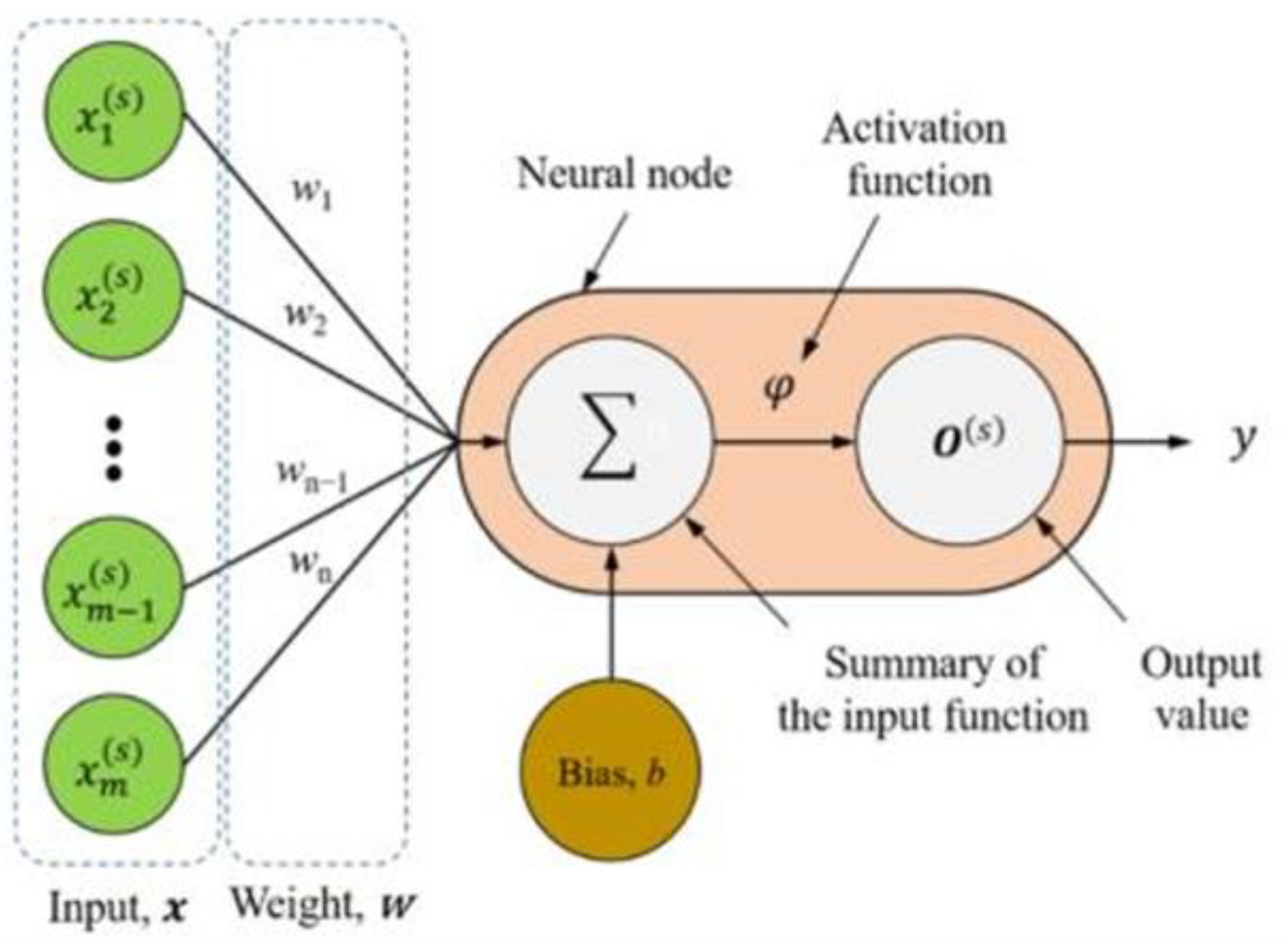
Figure 2.
Structure of the MLP.
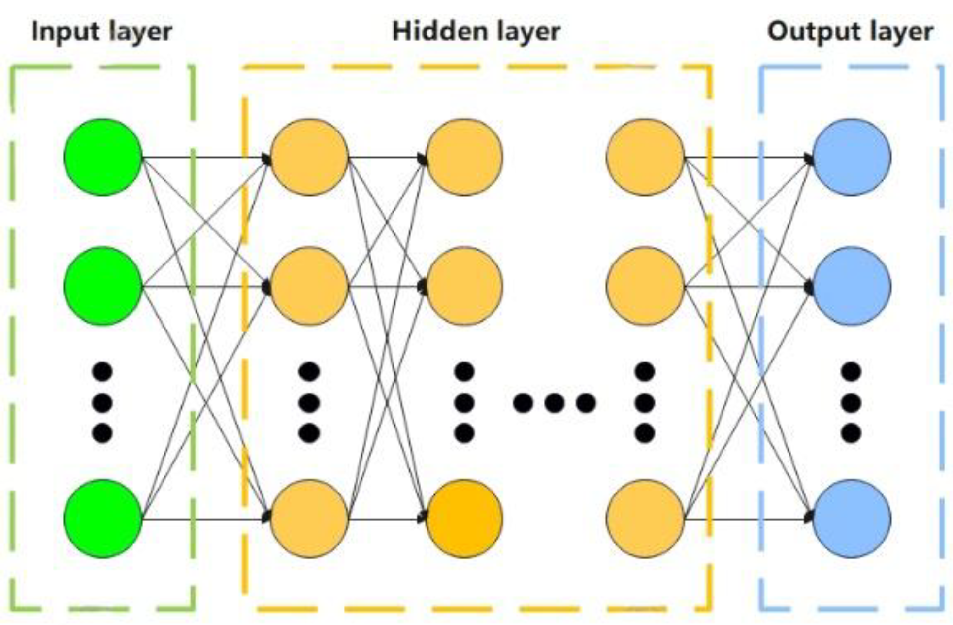
Figure 3.
CNN model diagram.
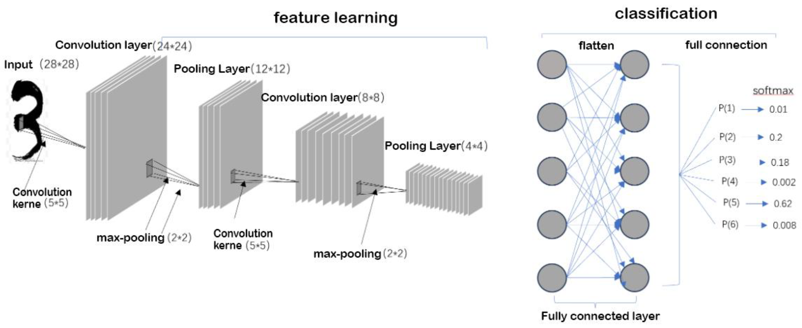
Figure 4.
AE model diagram.
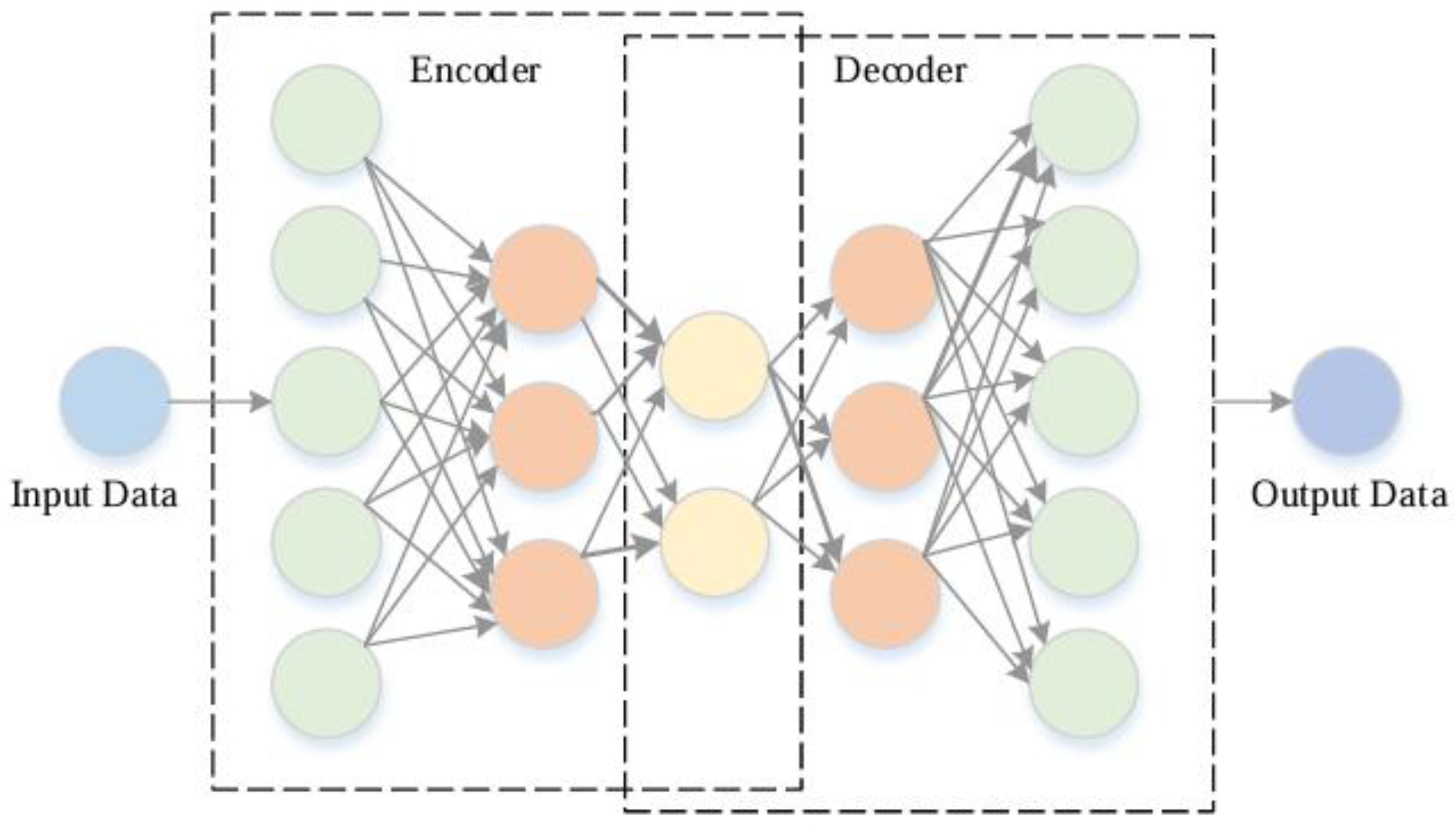
Figure 5.
RNN model diagram.
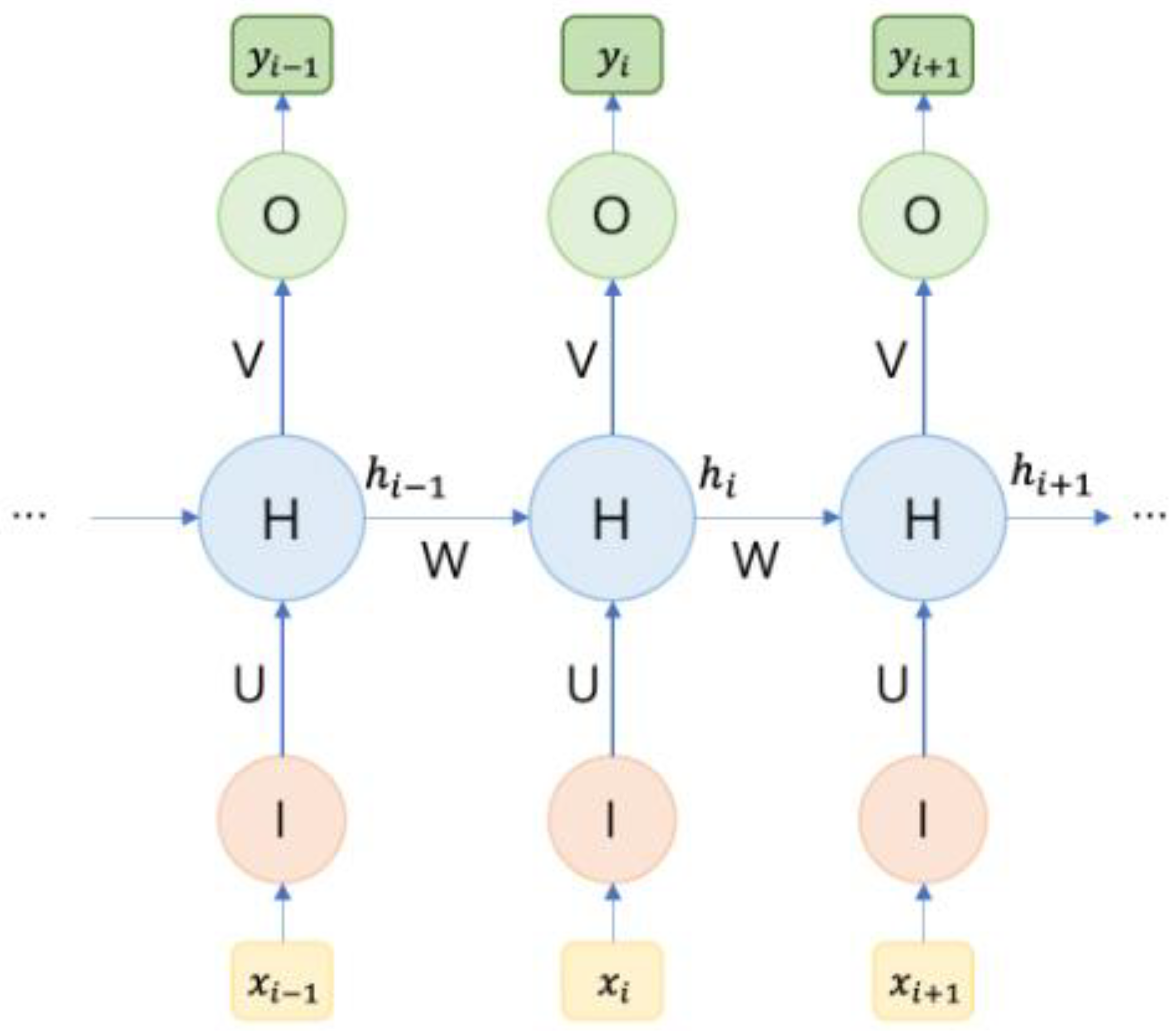
Figure 7.
GRU model diagram.
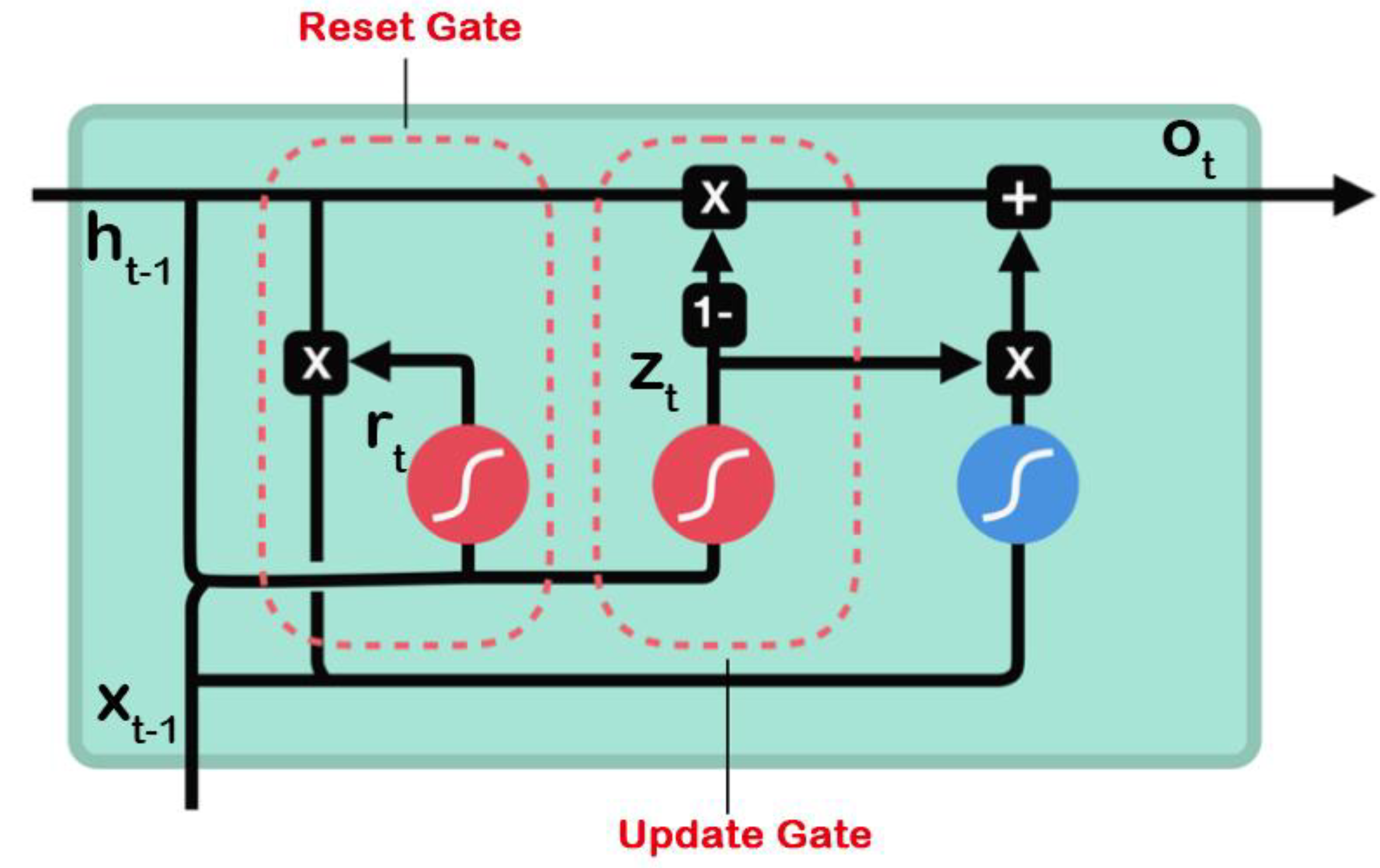
Figure 8.
Euclidean Structure Data and Non-Euclidean Structure Data structure diagram.
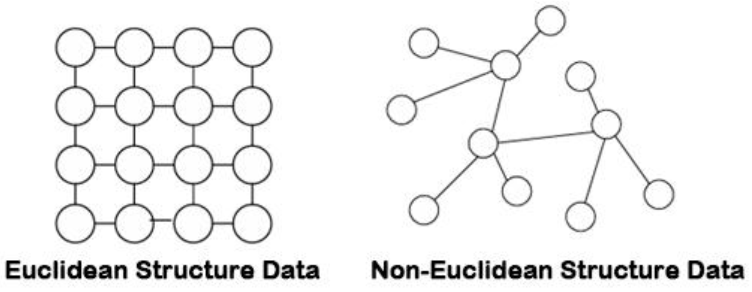
Figure 9.
Transformer model diagram.
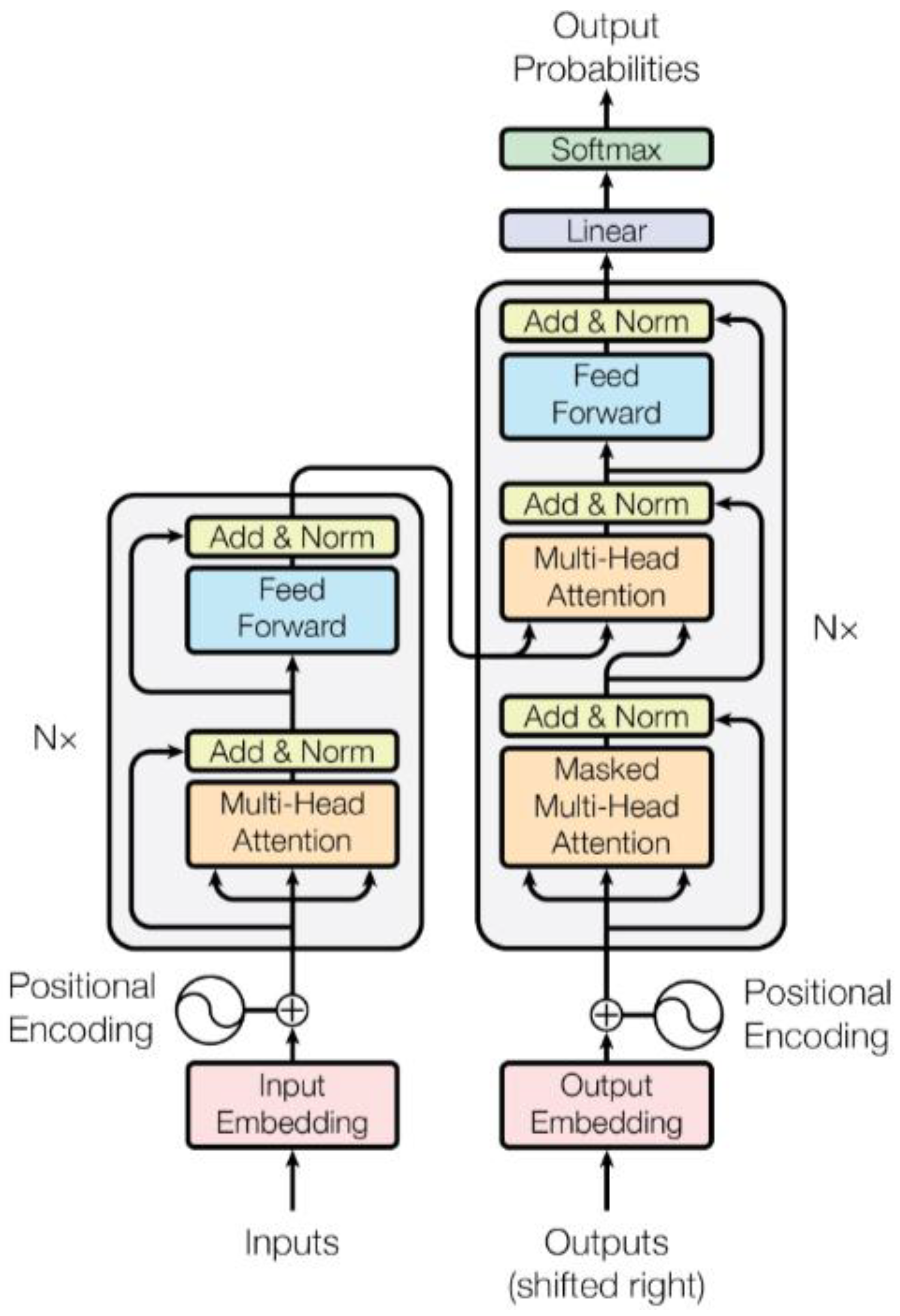
Figure 10.
DR model diagram.
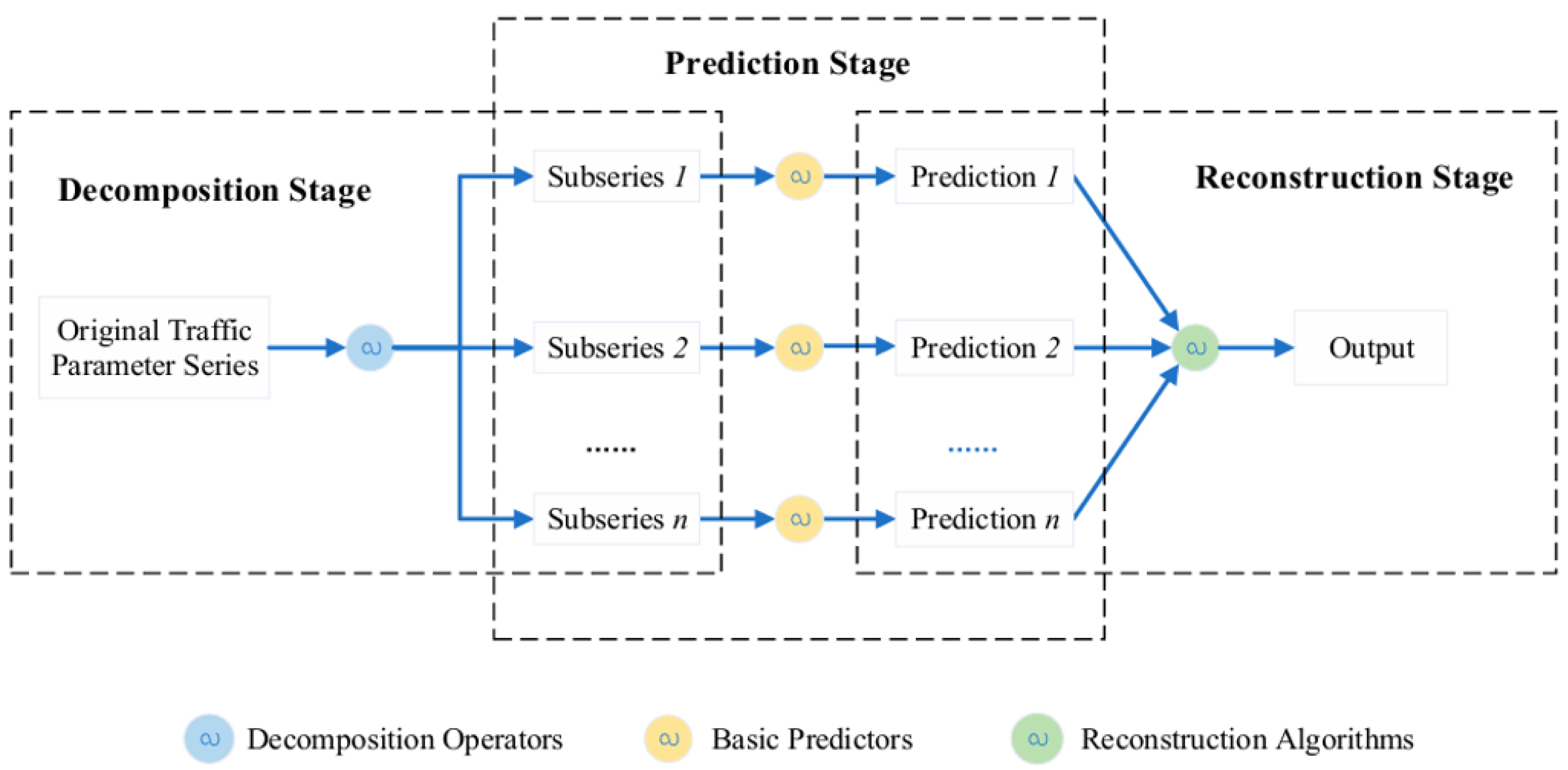

Table 1.
Dataset Summary.
| Type | Dataset | Features | Time interval | Traffic data | Source |
| Stationary traffic data | PeMS | Flow, speed | 5min | 39000 | https://github.com//Davidham3/ASTGCN |
| METR-LA | speed | 5min | 207 | https://github.com//liyaguang/DCRNN | |
| Loop | speed | 5min | 323 | https://github.com/zhiyongc/Seattle-Loop-Data | |
| UVDS | Flow, speed | 5min | 104 | [17] | |
| Mobile traffic data | TaxiBJ | Flow | 30min | 34,000 vehicles | https://github.com/TolicWang/DeepST/tree/master/data/TaxiBJ |
| SZ-taxi | Flow, speed | 15min | 156 roads | https://paperswithcode.com/dataset/sz-taxi | |
| NYC Bike | Flow | 60min | 13,000 bicycles | https://paperswithcode.com/dataset/nycbike1 | |
| Shanghai Taxi Dataset | speed | 1min | 4000 vehicles | https://www.cse.ust.hk/scrg/ |
Table 2.
Comparison of model performance on different datasets.
| Model | PEMS08 | METR-LA | ||
| MAE | RMSE | MAE | RMSE | |
| ARIMA | 33.04 | 50.41 | 2.04 | 5.89 |
| MLP | 26.73 | 35.81 | 1.84 | 4.62 |
| LSTM | 27.34 | 37.43 | 1.86 | 4.66 |
| GRU | 26.95 | 36.61 | 1.86 | 4.71 |
| ASTGCN | 19.63 | 27.50 | 1.31 | 3.54 |
Table 3.
Comparison of the advantages and disadvantages of different methods.
| Category | Model | Advantage | Disadvantages |
| Traditional statistical models | HA | The model algorithm is simple, runs fast, and has low execution time overhead | The model predicts future data based on the mean of historical data. Simple linear operations cannot represent the deep nonlinear relationship of spatiotemporal series. It is not ideal for predicting data with strong disturbance. |
| ARIMA | The model algorithm is simple and based on a large amount of uninterrupted data, this model has a high prediction accuracy and is particularly suitable for stable traffic flow. | Its modeling capability is relatively weak for nonlinear trends or very complex time series data, and is not suitable for non-stationary traffic flows. | |
| Kalman filter model | The algorithm is efficient, can process large amounts of data quickly, is adaptive, and can automatically adjust prediction results based on historical data, making it suitable for traffic flow prediction. | Because of its iterative nature, it requires continuous matrix operations, the algorithm has a large time overhead and cannot adapt to nonlinear changes in traffic flow. | |
| Machine Learning Models | KNN | High portability, simple principle, easy to implement. High model accuracy, good adaptability to nonlinear and non-homogeneous data. Suitable for short-term traffic status prediction | The processing efficiency of large-scale data sets is low, the model converges slowly, and the running time is long, which may not meet the requirements of real-time prediction of road traffic flow. |
| Deep Learning Models | MLP | The training process of MLP is relatively simple, and there are many optimization methods | The training process of MLP may take a long time and require high computing resources. When the amount of data or features are small, MLP may face overfitting problems. |
| CNN | CNN can effectively extract the spatial characteristics and temporal dependencies of traffic flow data, and has strong model generalization ability and high prediction accuracy. | Due to the complex structure of the model, the training process requires a lot of computing resources and time. At the same time, the structure of CNN cannot capture time dependencies well and has limited ability to process sequence data. | |
| AE | AE can learn the laws and patterns of historical traffic data to predict future traffic flow, which improves the efficiency and accuracy of traffic management. | For complex data distributions, training autoencoders can be difficult and requires careful tuning of the network structure and hyperparameters. | |
| RNN | RNN can capture the dynamic change characteristics of time series data, effectively use historical traffic flow information to predict future trends, and is suitable for processing traffic data with time dependence. | It is easy to encounter gradient vanishing or gradient exploding problems during training, making it difficult to effectively learn long-term dependencies. | |
| LSTM | LSTM’s unique gating mechanism can effectively alleviate the long-term dependency problem of traditional RNN, enabling the model to better capture long-term trends and cyclical changes in time series and improve prediction accuracy. | The LSTM model is relatively complex, takes a long time to train, and requires a large amount of historical data for training to achieve better results. | |
| GRU | GRU is simpler than LSTM, but it can also solve the problems of long-term dependence and gradient disappearance. | Its prediction performance is affected by data quality and feature selection. In complex scenarios, its prediction ability may be slightly inferior to LSTM. | |
| GCN | Good at processing non-Euclidean structure data, able to capture the relationship between nodes, and has good generalization ability | The computational resource requirements are high and overfitting may occur when processing large graphs | |
| Transformer | Transformer’s parallel computing capability greatly improves computational efficiency, and its self-attention mechanism enables the model to consider all positions in the sequence at the same time, thereby better capturing long-distance dependencies. | Requires a large amount of historical data for training, and the computational cost is high | |
| Hybrid Neural Network | Comprehensive learning and accurate prediction of traffic flow data can be achieved by combining the advantages of multiple neural network models. | The model is highly complex, and the training and optimization process is relatively difficult, requiring longer computing time and higher computing resources. |
Disclaimer/Publisher’s Note: The statements, opinions and data contained in all publications are solely those of the individual author(s) and contributor(s) and not of MDPI and/or the editor(s). MDPI and/or the editor(s) disclaim responsibility for any injury to people or property resulting from any ideas, methods, instructions or products referred to in the content. |
© 2025 by the authors. Licensee MDPI, Basel, Switzerland. This article is an open access article distributed under the terms and conditions of the Creative Commons Attribution (CC BY) license (http://creativecommons.org/licenses/by/4.0/).
Copyright: This open access article is published under a Creative Commons CC BY 4.0 license, which permit the free download, distribution, and reuse, provided that the author and preprint are cited in any reuse.


