
Submitted:
08 February 2025
Posted:
10 February 2025
You are already at the latest version
Abstract
In traffic flow prediction, many external factors, such as weather and holiday factors, have a significant impact on traffic flow. However, previous research on traffic flow prediction mainly focused on the internal correlations within traffic flow data, failing to integrate or comprehensively integrate the external factors affecting traffic flow to build prediction models. Based on this, this study collected as comprehensively as possible the data of external factors affecting traffic flow and integrated these data to construct a traffic flow prediction model. This study proposes a Temporal Graph Convolutional Network algorithm (IM - GCN), which comprehensively integrates multi - source heterogeneous external factors that affect traffic flow and for which collectable data are available, for traffic flow prediction modeling. This algorithm expands the receptive field of traffic flow features and enhances the reference weight of data with stronger correlations. The effectiveness of the proposed algorithm was verified through a large number of experiments on widely used traffic flow datasets. Experiments show that, compared with the state - of - the - art algorithms, on the premise that the increase in complexity reflected by the computational time consumption is less than 1%, the accuracy of the prediction model has been improved by 1% - 4%. Ablation experiments experimentally prove that the external factors affecting traffic flow added in this study can effectively improve the performance of the traffic flow prediction model.
Keywords:
traffic flow prediction
; GCN
; intelligent transportation
; multi-source data
; internet of vehicles
; predictive control
1. Introduction
1.1. Research Significance
With the continuous growth of urban population and the rapid increase in the number of urban vehicles, cities are facing increasingly severe problems such as traffic congestion, deterioration of traffic conditions, and environmental pollution [1]. This Intelligent Traffic System (ITS) serves as a comprehensive transportation network, seamlessly integrating advanced information technology, computer technology, data communication technology, sensor technology, artificial intelligence, and more, to enhance transportation and service control functions. It strengthens the connection among vehicles, roads, and users, thereby improving traffic efficiency, improving the environment, and saving energy. The application of the Intelligent Traffic System can effectively alleviate problems like traffic congestion [2]. Traffic flow prediction plays a crucial role within the intelligent traffic management system. It predicts the changes in traffic flow within a certain future time period by analyzing historical and real-time traffic data, including the prediction of data such as the number of vehicles, speed, and density on the road. Accurate traffic flow prediction is a necessary requirement for the effective operation of the intelligent traffic system, and the research on traffic flow prediction has significant practical and theoretical value [3].
Traffic flow exhibits significant spatial and temporal correlations. It is affected not only by the current traffic conditions upstream and downstream but also by historical traffic conditions. There is a non-linear and complex mapping relationship between traffic flow and various internal and external factors that influence it [4]. It is quite difficult to accurately predict traffic flow, and currently, what can be done is only to gradually improve the accuracy of traffic flow prediction. As a result, traffic flow prediction is rather challenging, which also makes it a traditional and enduring research topic all the time [5].
Deep learning is an important branch in the field of machine learning, specifically referring to networks with multiple non-linear transformation layers (deep networks). Since deep learning has networks with multiple non-linear transformation layers, deep learning methods are inherently better at capturing the complex mapping relationships of traffic flow than traditional traffic flow prediction methods [6].
With the continuous development of deep learning and its application in traffic flow prediction, along with the increasing availability of data that affects traffic flow and the application of Graph Convolutional Network (GCN) in traffic flow prediction, significant achievements have been made in traffic flow prediction. This has also made traffic flow prediction a hot topic that has been widely studied in recent years [7].
1.2. Definition and introd#uction
1.2.1. Definition of Traffic Flow Prediction
In traffic flow prediction, the urban road network space is generally defined as a weighted undirected graph, where is the set of road nodes, is the number of road nodes, and is the set of edges representing the relationships between road nodes. The input is the historical traffic flow dataset, and then the calculation of the next m steps of traffic information follows [8]. The traffic flow prediction result is denoted as , and the prediction process can be expressed by the following equation [8]:
Here, signifies the mapping relationship. The task of traffic flow prediction is to find out this mapping relationship.
1.2.2. Graph Convolutional Network
The Graph Convolutional Network (GCN) is an algorithm that uses neural networks to learn graph-structured data, extract and mine features and patterns in graph-structured data to meet the requirements of graph-learning tasks. In the research, the two-layer GCN model was used, which is represented by Equation (2) [9]:
Here, represents the output of the graph convolution operation, denotes the preprocessing matrix, and are learnable parameters, and are activation functions.
1.2.3. Gated Recurrent Convolution
The Gated Recurrent Unit (GRU for short) is a type of neural network structure designed to handle sequential data. It is an enhanced version of the Recurrent Neural Network (RNN). The GRU [10] addresses the issues of vanishing and exploding gradients that plague the Recurrent Neural Network (RNN). It utilizes the previous hidden state and the current flow information as inputs to ascertain the flow state at the present moment.
It has a simpler internal structure and lower training complexity compared to the Long Short-Term Memory (LSTM). The GRU can preserve the trends of historical traffic flow, and also capture the features of traffic flow at the current moment. The internal structure of the GRU network is shown in Figure 1 [11].
The formulas are shown as follows:
Among them, and respectively denote the update gate and the reset gate, is the candidate update state, and are activation functions, is the output state at the previous moment, is the input dataset at time t , and the parameters in the and series are all learnable parameters.
is the output value at t time. It can be seen from the above formula that can be used to determine how much of the output state at the previous moment should be discarded and how much new information of the candidate update state should be written in to derive the final output state.
1.2.4. T-GCN Model Based on Time-Domain Graph
The Temporal Graph Convolutional Network (T-GCN) models the time and space dependencies of traffic flow at the same time. The T-GCN model includes two parts: the Graph Convolutional Network (GCN) and the Gated Recurrent Unit (GRU). As shown in Figure 2, the T-GCN first takes the historical n time series data as input, uses the Graph Convolutional Network to capture the topological structure of the road network to obtain spatial features. Subsequently, the obtained time series data with spatial features is input into the Gated Recurrent Unit model, and the dynamic changes are obtained through the information transmission among the units, so as to capture the time features. Finally, we obtain the traffic flow prediction results through the fully connected layer [12].
1.3. Contributions of This Paper
Many external factors, such as weather conditions, holiday factors, day-of-the-week factors, Points of Interest (POI) factors, peak and off-peak traffic period factors, unexpected incidents on road sections, and temporary activities in road section areas, can all have a significant impact on traffic flow. In this study, weather factors, holiday factors, day-of-the-week factors, POI factors, and peak and valley traffic period factors are integrated for traffic flow prediction. However, the relevant data of road segment unexpected incidents and temporary activities in road segment areas cannot be collected, so these factors cannot be integrated. Nevertheless, so far, the IM-GCN model proposed in this study is still the traffic flow prediction model that integrates the most external factors.
Regarding the previous research on traffic flow prediction that did not integrate or only integrated a small number of external factors affecting traffic flow, the main contributions of this paper are as follows:
(1) In order to improve the accuracy of traffic flow prediction for complex urban roads, this study integrates the data affecting traffic flow, such as weather factors, Points of Interest (POI) factors in various regions, whether it is a holiday, day-of-the-week factors, and peak and off-peak traffic period factors, into the network. Then, the attribute information is combined with traffic characteristics to enhance the model's perception ability of external information, thereby improving the performance of traffic prediction, The IM-GCN algorithm proposed in this study is, so far, the algorithm that integrates the most external factors for traffic flow prediction.
(2) In order to achieve the prediction of real-time traffic conditions in complex traffic environments and also to integrate more data that is not directly related to traffic into the network, the network embedding algorithm is adopted. Through the embedding of spatial domain features and the embedding of temporal domain features, the network is enabled to handle more urban data, thereby improving the accuracy of deep learning models used for traffic flow prediction.
(3) In order to verify the contribution of the added external factors to traffic flow prediction, this study conducted ablation experiments. It was confirmed through the ablation experiments that the added external factors affecting traffic flow are helpful for improving the prediction accuracy.
2. Research Status and Existing Problems
The spatial interconnection of traffic flow is determined by the traffic network's topological layout. Upstream traffic conditions influence downstream ones via propagation, while downstream traffic conditions in turn impact upstream ones through feedback mechanisms. At the same time, traffic flow is also affected by time. The traffic flow state at a previous moment may affect the traffic flow state at a later moment. In most studies, time is emphasized while space is ignored. Therefore, it is necessary to model by combining the time-dependence and space-dependence of traffic flow, which avoids the dispersion of the entire traffic system and the destruction of the spatial dependence between nodes [13].
Figure 3 is a schematic diagram of the spatio-temporal correlation of traffic flow. A and B are two traffic flow monitoring points in the figure. t1, t2……tn, tn+1 are the various moments when traffic flow data is collected. In the figure, the traffic flow states of monitoring point A at moments t1, t2……tn may all have an impact on the traffic flow state of monitoring point B at moment tn+1 , which also represents the complex spatio-temporal correlation of traffic flow among various monitoring points [14].
2.1. Research Status
Currently, traffic flow prediction methods can be roughly divided into two major categories: classical methods and deep learning-based methods.
Classical methods include statistical methods and traditional machine learning methods. Statistical methods establish data-driven statistical models for prediction. The most representative algorithms are Historical Average (HA), Autoregressive Integrated Moving Average (ARIMA) [15], and Vector Autoregressive (VAR) [16]. In addition, some traditional machine learning methods, such as Support Vector Regression (SVR) [17] and Random Forest Regression (RFR) [18], are used for traffic flow prediction. These methods have the ability to handle high-dimensional data and capture nonlinear relationships.
The emergence of deep learning methods has greatly exploited the potential of artificial intelligence in traffic flow prediction [19]. This technology studies the use of hierarchical models to directly map the original input data to the expected output results [20]. Deep learning models stack basic learnable block layers to form a deep architecture, and the entire network is trained in an end-to-end manner. Currently, Convolutional Neural Networks (CNN) [21] are used to extract the spatial correlations of grid-structured data described by images or videos, while Graph Convolutional Networks (GCN) [22] extend the convolution operation to more general graph-structured data, which are more suitable for representing traffic network structures. Furthermore, Recurrent Neural Networks (RNN), along with its derivatives like Long Short-Term Memory Network (LSTM) and Gated Recurrent Unit (GRU), are commonly utilized for capturing temporal correlations. The integration of deep learning into traffic flow forecasting has led to substantial advancements in the field of traffic flow prediction [23,24,25].
2.2. Existing Problems
For traffic flow prediction methods that are based on statistics, there are specific assumptions that these methods need to satisfy. However, time-varying traffic data can hardly satisfy these assumptions. Moreover, these methods cannot be applied to large datasets. Therefore, it is difficult for traditional statistical methods to achieve high prediction accuracy [26]. For the methods based on traditional machine learning in traffic flow prediction, these methods have limited ability to handle nonlinear relationships, and it is hard for them to capture the spatio-temporal dependencies in traffic flow. They also lack comprehensive consideration of external factors that affect traffic flow. Hence, traditional machine learning methods are also difficult to obtain high prediction accuracy [27].
Although the application of deep learning methods in traffic flow prediction has achieved encouraging results, deep learning methods have problems such as overly long running time, which cannot guarantee the requirements of real-time prediction, poor model interpretability and insufficient generalization ability. Meanwhile, deep learning relies too much on the temporal correlation characteristics in short-term traffic flow prediction, while the relevant factors of spatial correlation characteristics are complex and difficult to quantify [28]. It is necessary to construct a spatial correlation measurement function that can simultaneously consider distance, traffic flow similarity and speed similarity to quantify the spatial correlation between prediction points and surrounding road sections. The collection of data that affects traffic flow, as well as how to process and reasonably integrate these heterogeneous data for traffic flow prediction, is also an important issue that urgently needs to be improved [29].
Zhao et al. [30] introduced the Temporal Graph Convolutional Network (T-GCN) model. In this model, the Graph Convolutional Network (GCN) was utilized to learn the intricate spatial topological structure in order to grasp the spatial features of traffic flow. Meanwhile, the Gated Recurrent Unit (GRU) was leveraged to learn the dynamic change characteristics of traffic data, thereby capturing the temporal attributes of traffic flow. The T-GCN model defined a smoothing filter in the Fourier domain, which made the variation of predicted values relatively small when the traffic flow reached its peak.
Yang et al. [31] considered the entire road as a complex road graph by employing the Graph Convolutional Network (GCN). They constructed a method for graph-level traffic flow prediction using the graph convolution network algorithm, thereby achieving predictions at the graph level for traffic flow. However, this method has problems such as insufficient receptive field, limited feature extraction ability and over-smoothing of predicted values.
Zhu et al. [32] put forward a knowledge representation-based traffic prediction method that utilizes the Spatio-Temporal Graph Convolutional Network. First, they constructed the traffic flow prediction and derived the knowledge expressions. Then, they put forward a knowledge fusion unit to combine traffic features as the input of the spatio-temporal graph convolution backbone network. This method has issues like insufficient consideration of external factors and how to effectively construct the knowledge graph.
Zhu et al. [33] proposed the Attribute-Augmented Spatio-Temporal Graph Convolutional Network (AST-GCN). They integrated external factors affecting traffic flow, such as weather factors and the distribution of surrounding Points of Interest (POI) as dynamic and static attributes, and designed an attribute expansion unit to encode and integrate these factors into the spatio-temporal graph convolution model to enhance the accuracy and anti-interference ability of prediction. Although this method integrates some external factors and improves the receptive field of the prediction model, it also has problems such as insufficient receptive field of the model and limited ability to capture traffic flow characteristics.
In terms of capturing the spatial dependence of traffic flow, Mou et al [34] used Convolutional Neural Networks (CNNs) to extract spatial features and combined them with Long Short-Term Memory Networks (LSTMs) to improve the prediction accuracy. CNNs are designed based on Euclidean-structured spaces, such as image grids. However, traffic flow has a non-Euclidean spatial structure. Therefore, they cannot essentially describe the spatial dependence of traffic flow. The newly emerged Graph Convolutional Networks (GCNs) can be used to model the spatial structure of traffic network sections. However, the models created by this method lack accuracy and robustness, and the generalization ability of the models is rather poor.
Wang et al. [35] proposed the ST-GCN method that can predict traffic flow without using historical data. On the basis of extracting spatio-temporal features by using the GCN and GRU methods, it combined the adjacency similarity algorithm to predict the traffic flow at intersections without using historical data. However, this method requires a large amount of historical data to train the model, ignores the dynamic traffic patterns of nodes, and is prone to the phenomenon of overfitting.
All in all, we need to build a traffic flow prediction model that integrates multiple external factors influencing traffic flow, increase the receptive field of the model, improve the current integration mechanism, and capture more traffic flow attributes, so as to enhance the accuracy of traffic flow prediction and the generalization ability of the prediction model.
3. Datasets Analysis and Collation
Apart from being influenced by the historical traffic flow conditions and the traffic flow conditions of upstream and downstream nodes, traffic flow can also be affected by a variety of external factors. Some of these external factors do not have collectable data, such as unexpected incidents on road sections and temporary activities. While some others have collectable data, like Point of Interest (POI) factors, weather factors, peak and off-peak time periods, day-of-the-week factors and holiday factors. In this study, the data of these external factors that affect traffic flow and are collectable will be comprehensively collected. The details of each type of data are introduced as follows.
3.1. POI Factors of Road Sections
Traffic flow is affected by the social attributes (Points of Interest, POI) of the area of the road section. According to the main social attribute characteristics of the road section, in this study, the road sections are divided into eight categories, namely commercial area sections, school area sections, residential area sections, hospital area sections, industrial area sections and so on. These eight characteristics are represented by the numbers 1 to 8 respectively in the POI dataset.
3.2. Weather Factors
Weather factors can have an impact on traffic flow. Regarding weather factors, based on the historical weather query data, this study divides the weather into twelve weather conditions, including sunny, cloudy, overcast, foggy, light rain, moderate rain, heavy rain, thundershower, sleet, light snow, heavy snow, and blizzard. A relevant dataset has been established and applied to traffic flow prediction. Moreover, weather factors are also one of the important factors affecting traffic flow. In this study, the dataset of weather conditions has been supplemented and improved. The weather conditions are divided into 12 characteristic values, and the dataset of weather conditions is integrated to model the traffic flow prediction model.
3.3. Morning and Evening Peak-Valley Factors
As shown in Figure 4, the traffic flow exhibits an obvious daily periodicity with morning and evening peak and valley periods, and this periodicity of morning and evening peak and valley is generally representative throughout the dataset.
In view of the obvious periodicity of morning and evening peak and valley periods in the traffic flow within a day, this study divides the peak and valley time periods in a day into six states, corresponding to the characteristic values of 1, 2, 3, 4, 5, and 6. The division method is shown in Table 1. Based on this table, a corresponding dataset regarding the peak and valley periods has been created, and this dataset has been applied to traffic flow prediction as an augmented matrix of traffic flow characteristics.
3.4. day-of-the-Week Factor
Traffic flow exhibits an obvious weekly periodicity. In response to this periodicity, this study distinguishes the characteristic of which day of the week the data was collected, dividing it into seven categories: Monday, Tuesday, Wednesday, Thursday, Friday, Saturday, and Sunday. A relevant dataset has been established and applied to traffic flow prediction.
Figure 5 shows the curve image of traffic flow in a week detected by a certain sensor in the PEMS04 traffic flow dataset. It can be seen from the figure that the data trends vary from Monday to Sunday.
We divide a week into seven characteristic values according to the days of the week, namely Monday, Tuesday, Wednesday, Thursday, Friday, Saturday, and Sunday. To further quantify the difference in traffic flow data at the same time between the day-of-the-week and other days, we adopted the algorithm shown in Figure 6.
In Figure 6, the "data.csv" dataset is the traffic flow dataset, and the "weeklyday.csv" dataset is the dataset regarding the data collected on a certain day-of-the-week. Both are two-dimensional data. The illustrated algorithm calculates the mean absolute error and root mean square error of the traffic flow data at the same time point in a day when it is a same day-of-the-week but is not a same day. The results are listed in Table 2. By using a similar algorithm, we can calculate the mean absolute error and root mean square error of the traffic flow data at the same time point in a day between when it is not a same day-of-the-week, and the results are listed in Table 2.
For a better understanding of Table 2, here is an example. The number 30 in the second row and the third column of Table 2 represents the mean absolute error of traffic flow data at the same time on each Monday compared with that on other Mondays. And the number 67 in the fifth row and the third column of Table 2 represents the root-mean-square deviation of traffic flow data at the same time point on each Monday compared with that on non-Mondays. It can be seen from Table 2 that the difference in data among the days of the same day-of-the-week is significantly smaller than that at the same time among the days that are not of the same day-of-the-week.
Through the above comparison of data differences, in view of the phenomenon that the difference between traffic data on the days of the same day-of-the-week and those on the days that are not of the same day-of-the-week is greater, this study established a dataset indicating on which day of the week each piece of traffic flow data was collected. This dataset has seven characteristic values, and integrated this dataset into the traffic flow prediction modeling. Experiments have proved that the established model has improved the prediction accuracy.
3.5. Holiday Factors
It can be seen from Figure 5, the traffic flow trends on working days from Monday to Friday are clearly different from those on weekends. Given that the traffic flow on holidays and working days shows significantly distinct characteristics, this study differentiates among three states, namely working days, weekends, and holidays, and has established a dataset with three characteristic values for working days, weekends, and holidays. This dataset is used to record whether the traffic flow data is collected on working days, weekends, or holidays. The relevant dataset has been established and applied to traffic flow prediction.
4. Methods of Data Fusion
4.1. Fusion of External Factors Affecting Traffic Flow
Figure 7 is a schematic diagram of modeling by fusing datasets of weather, day-of-the-week, regional points of interest, holidays, and peak and valley time periods. After fusion these external factors affecting traffic flow, they are preprocessed together with the traffic flow data and then input into the T-GCN traffic flow prediction model.
Figure 8 shows the pseudo code diagram of the data fusion algorithm for external factors affecting traffic flow. In this data fusion algorithm, POI data, weather data, peak-valley data, day-of-the-week data and holiday data are all external factors that affect traffic flow and for which data can be collected. This algorithm first cascades these external data to form a comprehensive matrix, and then uses two-dimensional convolution operations one by one according to the time span and node range to extract the internal features of these data. After the cascading operation, it stacks with the traffic flow data to form the data after feature fusion.
4.2. Embedding of Spatial Features of External Factors
Network embedding refers to mapping low-dimensional, dense and real-valued vectors in a network to a K-dimensional hidden space. Here, network embedding is used to fuse external factors that have no direct relationship with traffic. It takes external factor data such as Point of Interest (POI) data, weather data, peak-valley data, day-of-the-week data and holiday data as inputs to obtain the feature matrix, as shown in Figure 9.
In Figure 9, field_m represents m different external factors, here, m = 5. Each factor is encoded with 0 and 1 to form a feature matrix. For one of the nodes, the dimension of the matrix is [m, k], here, k = 5. Then, the embedded feature vector W is multiplied by it to obtain a dense feature matrix with real values. Here, W can be learned as a network parameter, and all nodes share the embedded vector W.
4.3. Embedding of the Temporal Attributes of External Factors
To capture the time-varying characteristics of factors that have no direct relationship with traffic, we divide a day into T time periods according to the step length of traffic flow. For all time periods of each day, we use a T×k×k tensor Wt to represent the variation of factors that have no direct relationship with traffic flow. Wt is represented as a temporal feature embedding vector. Among them, Wt can be self-learned as a network parameter, and its size is only related to the length of the time period and the length of the embedding vector, and has nothing to do with the number of nodes.
Figure 10 shows the extraction of temporal features in the calculation. Among them, the input is the time factor t, which is converted into a one-hot encoding with a length equal to T. Then, combined with Wt, the temporal embedding vector corresponding to time t is extracted through the embedding process to obtain the representation of the temporal feature:
Among them, represents the lookup function. represents the data at time t that has been found.
4.4. The Overall Framework of the Algorithm
On the basis of spatio-temporal graph convolution, this study adopts a spatio-temporal graph convolution model based on data fusion. This model takes the data fused from spatial feature embedding and temporal feature embedding as an attribute enhancement unit and forms an attribute enhancement matrix with the original data. As shown in Figure 11.
In Figure 11, after the cascading operation on the data of the five external factors that affect traffic flow and have been collected, the function is used to extract the data at time t. Then, a two-dimensional convolution operation is performed on each node one by one. After the operation of the activation function, the traffic flow historical data are cascaded for data preprocessing. After preprocessing, data groups grouped according to the length of the historical data and the length of the data to be predicted are obtained, which are distinguished as the training dataset (trainX) and the train label dataset (trainY), as well as the testing dataset (testX) and the testing label dataset (testY). The obtained datasets after feature fusion and grouping are used as the input of the TGCN model. Combined with the preprocessed road node connection matrix, the TGCN model is trained and the traffic flow prediction values are calculated.
5. Experimental Verification
5.1. Experimental Data Set
The following data sets were used in this experiment:
SZ-taxi Data Set:This dataset is the Shenzhen taxi trajectory dataset from January 1st to 31st, 2015. It includes monitoring points on 156 main roads in Luohu District, Shenzhen, and records vehicle information data at 15-minute intervals. Meanwhile, it also records five external datasets that affect traffic flow, namely the Points of Interest (POI) dataset, the weather dataset, the day-of-the-week dataset, the holiday dataset, and the morning and evening traffic peak and off-peak dataset. The POI types are classified into nine categories: catering, commerce, transportation, education, medicine, etc. The main types among them correspond to the POI characteristics of road sections. The weather data is divided into five types: cloudy, light rain, fog, sunny, and heavy rain. In this study, datasets of the day-of-the-week, holidays, and traffic peak and valley periods within a day were supplemented. The source data can be obtained from the website: https://github.com/lehaifeng/T-GCN/tree/master/data.
The PEMS04 Data Set: This data set describes the San Francisco Bay Area, covering 3848 sensors on 29 roads. It contains traffic flow information for 59 days from January 1st to February 28th, 2018, with flow information recorded at five-minute intervals at each monitoring point. It also includes data information about the day-of-the-week. In this study, corresponding regional weather data sets, holiday data sets, and traffic flow peak and valley period data sets within a day were supplemented. The source data set can be obtained from thewebsite: https://github.com/Davidham3/ASTGCN/tree/master/data/ PEMS04.
5.2. Evaluation Metrics
We selected the following four performance metrics to assess the differences between the actual and predicted results. Root-Mean-Square Error (RMSE) and Mean Absolute Error (MAE) are used to measure the prediction error. Accuracy (ACC) is used to detect the prediction accuracy, and the coefficient of determination R2 is calculated to measure the ability of the predicted results to fit the actual data.
In the above equation, represents the actual traffic flow of the i-th road section during the j-th time interval; denotes the predicted traffic flow of the i-th road section in the j-th time interval; is the actual value of the sample; is the predicted value of the model; is the average value of the sample; M signifies the total count of time periods in the sample, while N indicates the number of nodes that constitute the road.
5.3. Loss Function
The purpose of training is to minimize the error between the real speed and the predicted speed in the road network. The real speed and the predicted speed at different cross-sections at time t are represented by and respectively. Therefore, the objective function in this paper is shown as follows.
Among them, and are the ground truth and prediction. The second term represents the regularization term for avoiding overfitting, and λ is a hyperparameter.
5.4. Parameterization
The model's learning rate is configured at 0.01, with a batch size of 64 and a total of 2000 epochs. Regularization techniques are applied to guard against overfitting. A 70% portion of the entire dataset is allocated for training input, while the rest serves as testing input. The Adam optimization algorithm is utilized for model training.
The main platforms used in the experiment are Python 3.6.0, TensorFlow 1.15.0, PyCharm, and Windows 10.
5.5. Experimental Result Analysis and Comparison
In this study, the ARIMA algorithm, the AST_GCN algorithm, the T_GCN algorithm, and the IM-GCN algorithm proposed in this paper were used to make predictions on the SZ-taxi data set and the PEMS04 data set. The initial 70% portion of the dataset was utilized as the training set, while the leftover 30% served as the testing set. The outcomes and analysis of the experiment are presented below.
Figure 12 shows the comparison between the predicted values and the actual values obtained by using the IM-GCN, AST_GCN, T_GCN, and ARIMA algorithms respectively to predict the SZ-taxi data set. In the figure, the blue solid line represents the curve of the actual traffic flow values, and the red solid line represents the traffic flow predicted values obtained by the IM-GCN algorithm proposed in this paper. It can be seen from the figure that since the algorithm proposed in this paper integrates data from multiple aspects more comprehensively for prediction and has a larger receptive field, the IM-GCN algorithm achieves the best prediction accuracy. The AST_GCN obtains the second-best prediction performance, and the traditional ARIMA algorithm has the lowest prediction accuracy.
In this paper, the data of the previous 10 time steps (with each time step being 15 minutes) is utilized to predict the next time step, using the SZ-taxi data set. When predicting one time step, the prediction results of the model are shown in Table 3. Moreover, the proposed model in this paper is compared with models such as ARIMA, HA, SVR, GCN, T-GCN, and AST-GCN. It can be seen that the prediction model proposed in this paper is superior to the baseline models in all aspects.
It can be seen from Table 3 that the RMSE and MAE values of the IM-GCN model are smaller than those of other models, while its accuracy (ACC) and the coefficient of determination R2 are higher, indicating that the IM-GCN model has better prediction performance and higher accuracy. Especially in time series prediction problems, compared with traditional statistical methods (such as ARIMA), the IM-GCN model has stronger prediction ability, with an improvement of more than 40% in test performance. This may be due to the limitations of traditional methods when dealing with such high-complexity data.
Compared with the second-best model AST-GCN, the prediction results of the IM-GCN model in terms of RMSE, MAE, ACC, and R2 have been improved by 2.83%, 3.8%, 2.38%, and 1.89% respectively.
Figure 13 is a comparison chart of the predicted values and the actual values obtained by using the IM-GCN, AST_GCN, T_GCN, and ARIMA algorithms respectively to predict the PEMS04 dataset. In the figure, the blue solid line represents the curve of the actual traffic flow values, and the red solid line represents the traffic flow predicted value curve obtained by the IM-GCN algorithm proposed in this paper. It can be seen from the figure that the IM-GCN algorithm achieves the best prediction accuracy, the AST_GCN obtains the second-best prediction performance, and the traditional ARIMA algorithm has the lowest prediction accuracy.
It can be seen from the data in Table 4 that the RMSE and MAE values of the IM-GCN model are smaller than those of other models, indicating that the IM-GCN model has better prediction performance and higher accuracy. Compared with the second-best model, the prediction results of MAE, MAPE (Mean Absolute Percentage Error), and RMSE are improved by 1.54%, 2.81%, and 1.41% respectively.
The AST-GCN model only concatenates some external factors that affect traffic flow with traffic information and fails to comprehensively capture the connections among these pieces of information. The IM-GCN model proposed in this paper captures the spatio-temporal characteristics of external information by embedding comprehensive traffic flow information, thus improving the prediction performance of the model.
Based on 1,000 iterations, the model in this paper is compared with the AST-GCN. As shown in Table 5, the model in this paper is slightly superior to the AST-GCN in all aspects.
Table 5 shows the performance evaluation results of three models (T-GCN, AST-GCN and IM-GCN) on the SZ_taxi dataset under different time ranges (15 minutes, 30 minutes, 45 minutes and 60 minutes). Based on Table 5, it can be seen that the IM-GCN model outperforms the T-GCN and AST-GCN models in all time ranges. Specifically, within the prediction ranges of 45 and 60 minutes, compared with the T-GCN model, the IM-GCN model shows that the RMSE is reduced by 2.15% and 1.87%, respectively, and the MAE is reduced by 3.51% and 2.44%, respectively. The RMSE of the IM-GCN model is reduced by 1.24% and 1.17% compared with the AST-GCN model, respectively, and the MAE is reduced by 1.40% and 1.40% compared with the AST-GCN model, respectively, with a decrease of 1.40% and 1.19% respectively. It is worth noting that the prediction performance of all models declines as the time interval increases. This is because as the time interval increases, the prediction task becomes more difficult, and the model needs to capture the changes in data over a longer time range, which may lead to overfitting and an increase in prediction errors. However, although the performance of the metrics declines, the decline is not significant, indicating that the models possess a certain degree of robustness and prediction ability.
5.6. Ablation Experiment
In order to verify the necessity of conducting experiments by adding each external factor that affects traffic flow, this study carried out ablation experiments on weather factors, distribution factors of surrounding Points of Interest (POI), day-of-the-week factors, holiday factors, and morning and evening rush hour factors respectively.
Figure 14 is the curve graph of the predicted values obtained from the ablation experiment on the external factors affecting traffic flow by the IM-GCN algorithm. This experiment was conducted using the PEMS04 traffic flow data set. After the predicted data was input into the evaluation index formula and calculated, the values of each evaluation index are shown in Table 6.
Table 6 is a table comparing the performance metrics of the models in the ablation experiments on various factors affecting traffic flow in the PEMS04 data set. It can be seen from the table that when the weather factor is not considered, the mean absolute error increases by 2.95 and the mean absolute percentage error increases by 1.73%. When the holiday factor is not considered, the mean absolute error increases by 2.58 and the mean absolute percentage error increases by 1.4%. Based on this table, it can be seen respectively that when the weather factor, holiday factor, weekday factor, POI factor, and traffic peak and trough period factor are ablated individually, the performance metrics of the prediction model all decline to varying degrees.
The ablation experiments in this study demonstrate that integrating the external factors affecting traffic flow, namely weather factors, holiday factors, weekday factors, POI factors, and traffic peak and trough period factors, for traffic flow prediction can effectively improve the performance of the prediction model. In other words, in order to obtain a more accurate traffic flow prediction model, it is necessary to integrate these external factors.
5.7. Comparison of the Computational Complexity of Algorithms
In this study, the computational complexity of algorithms is measured by the computing time consumption per iteration. The SZ-taxi data set is adopted in this study. Under the condition that each algorithm runs for 1,000 iterations, the average time consumption per iteration is calculated, and the list is shown in Table 7.
It can be seen from Table 7 that, compared with the current state-of-the-art AST-GCN algorithm, the proposed algorithm IM-GCN in this study takes 1% more time per iteration than AST-GCN. However, the prediction results of the model performance metrics RMSE, MAE, ACC, and R2 are improved by 2.83%, 3.8%, 2.38%, and 1.89% respectively. It can be observed that the increase in computational complexity brought about by the integration of more multivariate data in the IM-GCN algorithm proposed in this paper is negligible.
6. Conclusion and Future Work
This study presents a model that integrates heterogeneous data as comprehensively as possible for predicting traffic flow, aiming to address the limitations of traditional urban traffic flow prediction models in failing to comprehensively consider the impact of external factors on traffic. Unlike simple integration methods, our model effectively captures static and dynamic external information by fully integrating external information related to traffic flow through embedding in the time and spatial domains. Through comparison with baseline methods, the algorithm proposed in this paper improves the accuracy of traffic flow prediction with almost no increase in algorithm complexity, and enriches the research on the impact of external factors on traffic flow. However, the impact on traffic flow is not limited to the factors mentioned in this paper. For example, unexpected incidents and temporary activity factors can also have an impact on traffic flow. Due to limitations in the sources of datasets, this study was unable to obtain corresponding datasets. These issues can be further explored in future research.
Traffic flow prediction is a process of continuous improvement in accuracy. In our future research, in order to predict traffic flow more accurately, on the one hand, we can try to collect more types of data on external factors that affect traffic flow for traffic flow prediction. On the other hand, we can explore the use of more effective data fusion methods to discover the internal relationships among data more effectively.
Author Contributions
: Conceptualization, G.Y. and X.F.; methodology, G.Y. and X.F.; software, G.Y. and S.L.; validation, G.Y. and Y.X.; formal analysis, G.Y.; data curation, Y.L.; writing—original draft preparation, G.Y. All authors have read and agreed to the published version of the manuscript.
Funding
This work was supported in part by Project of the Ministry of Science and Technology(2022041009L),in part by the key research and development plan of Shaanxi province (2021GY-072).
Institutional Review Board Statement
Not applicable.
Informed Consent Statement
Not applicable.
Data Availability Statement
All the data used to support the findings of this study are included within the article.
Acknowledgments
Thank you to the alumni of Liaoning University of Technology for assisting in providing traffic volume data for the survey of Jinzhou City, China.
Conflicts of Interest
The authors declare no conflict of interest.
References
- Barros, J.; Araujo, M.; Rossetti, R. J. F. Short-term real-time traffic prediction methods: A survey. 2015 International Conference on Models and Technologies for Intelligent Transportation Systems (MT-ITS), Budapest, Hungary 3-6 June 2015.
- Tian, Y. and Pan, L. Predicting Short-Term Traffic Flow by Long Short-Term Memory Recurrent Neural Network. 2015 IEEE International Conference on Smart City/SocialCom/SustainCom (SmartCity), Chengdu, China, 19-21 December 2015.
- Tuna, E. and Soysal, A. LSTM and GRU based Traffic Prediction Using Live Network Data. 2021 29th Signal Processing and Communications Applications Conference (SIU), Istanbul, Turkey, 9-11 September 2021.
- Bao, Yinxin; Huang, Jiashuang; Shen, Qinqin; Cao, Yang; Ding, Weiping; Shi, Zhenquan; Shi, Quan. Spatial–Temporal Complex Graph Convolution Network for Traffic Flow Prediction. Engineering Applications of Artificial Intelligence. 2023, 121, 1-16.
- Liu, Y.; Zheng, H.; Feng, X. and Chen, Z. Short-term traffic flow prediction with Conv-LSTM. 2017 9th International Conference on Wireless Communications and Signal Processing (WCSP), Nanjing, China, 11-13 October 2017.
- Liao, W.; Bak-Jensen, B.; Pillai, J. R.; Wang Y. and Y. Wang. A Review of Graph Neural Networks and Their Applications in Power Systems. Journal of Modern Power Systems and Clean Energy. 2022, 10, 345-360.
- Hochreiter S. and Schmidhuber J. Long short-term memory. Neural Comput. 1997, 9, 1735–1780.
- Fu, R.; Zhang, Z. and Li, L. Using LSTM and GRU neural network methods for traffic flow prediction. 2016 31st Youth Academic Annual Conference of Chinese Association of Automation (YAC), Wuhan, China, 13-15 October 2016.
- Lai, Q.; Tian, J.; Wang, W.; Hu, X. Spatial–temporal attention graph convolution network on edge cloud for traffic flow prediction. IEEE Trans. Intell. Transp. Syst. 2023, 24, 4565–4576.
- Lana, I.; DelSer, J.; Velez, M. and Vlahogianni, E. I. Road Traffic Forecasting: Recent Advances and New Challenges. IEEE Intelligent Transportation Systems Magazine. 2018, 10, 93-109.
- Berlotti, M.; Grande, S. D. and Cavalieri, S. Proposal of a machine learning approach for traffic flow prediction. Sensors, 2024, 24(7), 2348.
- Mohammed, A. R.; Mohammed, S. A. and Shirmohammadi, S. Machine Learning and Deep Learning Based Traffic Classification and Prediction in Software Defined Networking. 2019 IEEE International Symposium on Measurements & Networking (M&N), Catania, Italy, 8-10, July 2019.
- Zhang, J.; Wang, F. -Y.; Wang, K.; Lin W. -H.; Xu X. and Chen C. Data-Driven Intelligent Transportation Systems: A Survey. IEEE Transactions on Intelligent Transportation Systems. 2011, 12, 1624-1639.
- Wang, H.; Zhang, R.; Cheng, X. and Yang, L. Hierarchical traffic flow prediction based on spatial–temporal graph convolutional network. IEEE Trans. Intell. Transp. Syst. 2022, 23, 16137–16147.
- Waheeb, W.; Ghazali, R. and Shah, H. Nonlinear Autoregressive Moving-average (NARMA) Time Series Forecasting Using Neural Networks. 2019 International Conference on Computer and Information Sciences (ICCIS), Sakaka, Saudi Arabia, 3-4 April 2019.
- Hasanah, R. N.; Ravie, R. P.; O.M.P. and Suyono, H. Comparison Analysis of Electricity Load Demand Prediction using Recurrent Neural Network (RNN) and Vector Autoregressive Model (VAR). 2020 12th International Conference on Electrical Engineering (ICEENG), Cairo, Egypt, 7-9 July 2020.
- Chen, R.; Liang C.-Y.; Hong W.-C. and Gu D.-X. Forecasting holiday daily tourist flow based on seasonal support vector regression with adaptive genetic algorithm. Appl. Soft Comput. 2015, 26, 435–443.
- Johansson, U.; Boström, H.; Löfström, T. and Linusson, H. Regression conformal prediction with random forests. Mach. Learn. 2014, 97,155–17.
- Lv, Y.; Duan, Y.; Kang, W.; Li, Z. and Wang, F.-Y. Traffic flow prediction with big data: A deep learning approach. IEEE Trans. Intell. Transp. Syst. 2015, 16, 865–873.
- Li, D.; Zhao, X.; Cao, P. An enhanced motorway control system for mixed manual/automated traffic flow, IEEE Syst. J. 2020, 14(4), 4726-4734.
- Ma, Q.; Huang, G.H. and Ullah, S. A Multi-Parameter Chaotic Fusion Approach for Traffic Flow Forecasting. IEEE Access. 2020, 8, 222774-222781.
- Zou, G.; Lai, Z.; Wang, T.; Liu, Z.; Li, Y. MT-STNet: A Novel Multi-Task Spatiotemporal Network for Highway Trafffc Flow Prediction. IEEE TRANSACTIONS ON INTELLIGENT TRANSPORTATION SYSTEMS. 2024, 25, 8221-8236.
- Liu, S.; Lin, Y.; Luo, C. and Shi, W. A Novel Learning Method for Traffic Flow Forecasting by Seasonal SVR with Chaotic Simulated Annealing Algorithm. 2021 IEEE 6th International Conference on Computer and Communication Systems (ICCCS), Chengdu, China, 23-26 July 2021.
- Qi, X.; Mei, G.; Tu, J.; Xi N. and Piccialli, F. A Deep Learning Approach for Long-Term Traffic Flow Prediction With Multifactor Fusion Using Spatiotemporal Graph Convolutional Network. IEEE Transactions on Intelligent Transportation Systems. 2023, 24, 8687-8700.
- Awan, A. A.; Majid, A.; Riaz, R.; Rizvi, S. S. and Kwon, S. J. A Novel Deep Stacking-Based Ensemble Approach for Short-Term Traffic Speed Prediction. IEEE Access, 2024, 12, 15222-15235.
- Zhao, B.; Gao, X.; Liu, J.; Zhao, J. and Xu, C. Spatiotemporal Data Fusion in Graph Convolutional Networks for Traffic Prediction. IEEE Access. 2020, 8, 76632-76641.
- Zheng, Y.; Li, W.; Zheng, W.; Dong, C.; Wang, S. and Chen, Q. Lane-level heterogeneous traffic flow prediction: A spatiotemporal attention-based encoder–decoder model. IEEE Intell. Transp. Syst. Mag., 2023, 15, 51–67.
- Li, L.; Zhou, X.; Hu, G.; Li, S. and Jia, D. A Recurrent Spatio-Temporal Graph Neural Network Based on Latent Time Graph for Multi-Channel Time Series Forecasting. IEEE Signal Processing Letters, 2024, 31, 2875-2879.
- Yang, D. and Lv, L. A Graph Deep Learning-Based Fast Traffic Flow Prediction Method in Urban Road Networks. IEEE Access, 2023, 11, 93754-93763.
- Zhao, L.; Song, Y.; Zhang, C. et al. T-GCN: A Temporal Graph Convolutional Network for Traffic Prediction. IEEE Transactions on Intelligent Transportation Systems, 2019, 21(9), 3848-3858.
- Yang, G.; Yu, H. and Xi, H. A Spatio-Temporal Traffic Flow Prediction Method Based on Dynamic Graph Convolution Network. 2022 34th Chinese Control and Decision Conference (CCDC), Hefei, China, 15-17 August 2022.
- Zhu, J. et al. KST-GCN: A Knowledge-Driven Spatial-Temporal Graph Convolutional Network for Traffic Forecasting. IEEE Transactions on Intelligent Transportation Systems, 2022, 23(9), 15055-15065.
- Zhu J.; Wang Q.; Tao C.; Deng H.; Zhao L. and Li H. AST-GCN: Attribute-Augmented Spatiotemporal Graph Convolutional Network for Traffic Forecasting. IEEE Access, 2021, 9, 35973-35983.
- Mou, L.; Zhao P.; Xie, H. and Chen, Y. T-LSTM: A Long Short-Term Memory Neural Network Enhanced by Temporal Information for Traffic Flow Prediction. IEEE Access, 2019, 7, 98053-98060.
- Wang, Y.; Zheng, J.; Du, Y.; Huang, C. and Li, P. Traffic-GGNN: Predicting Traffic Flow via Attentional Spatial-Temporal Gated Graph Neural Networks. IEEE Transactions on Intelligent Transportation Systems, 2022, 23, 18423-18432.
Figure 1.
Diagram of the Gated Recurrent Unit Network Structure
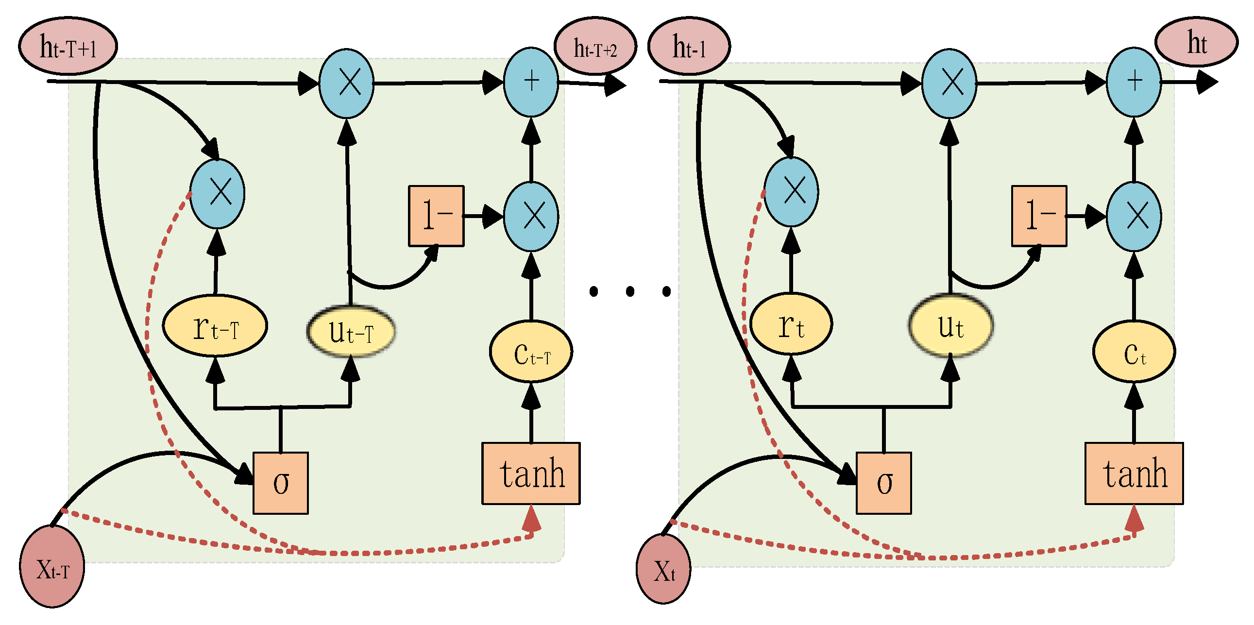
Figure 2.
Framework Diagram of the T-GCN Algorithm.

Figure 3.
Schematic Diagram of the Spatio - Temporal Correlation of Traffic Flow.
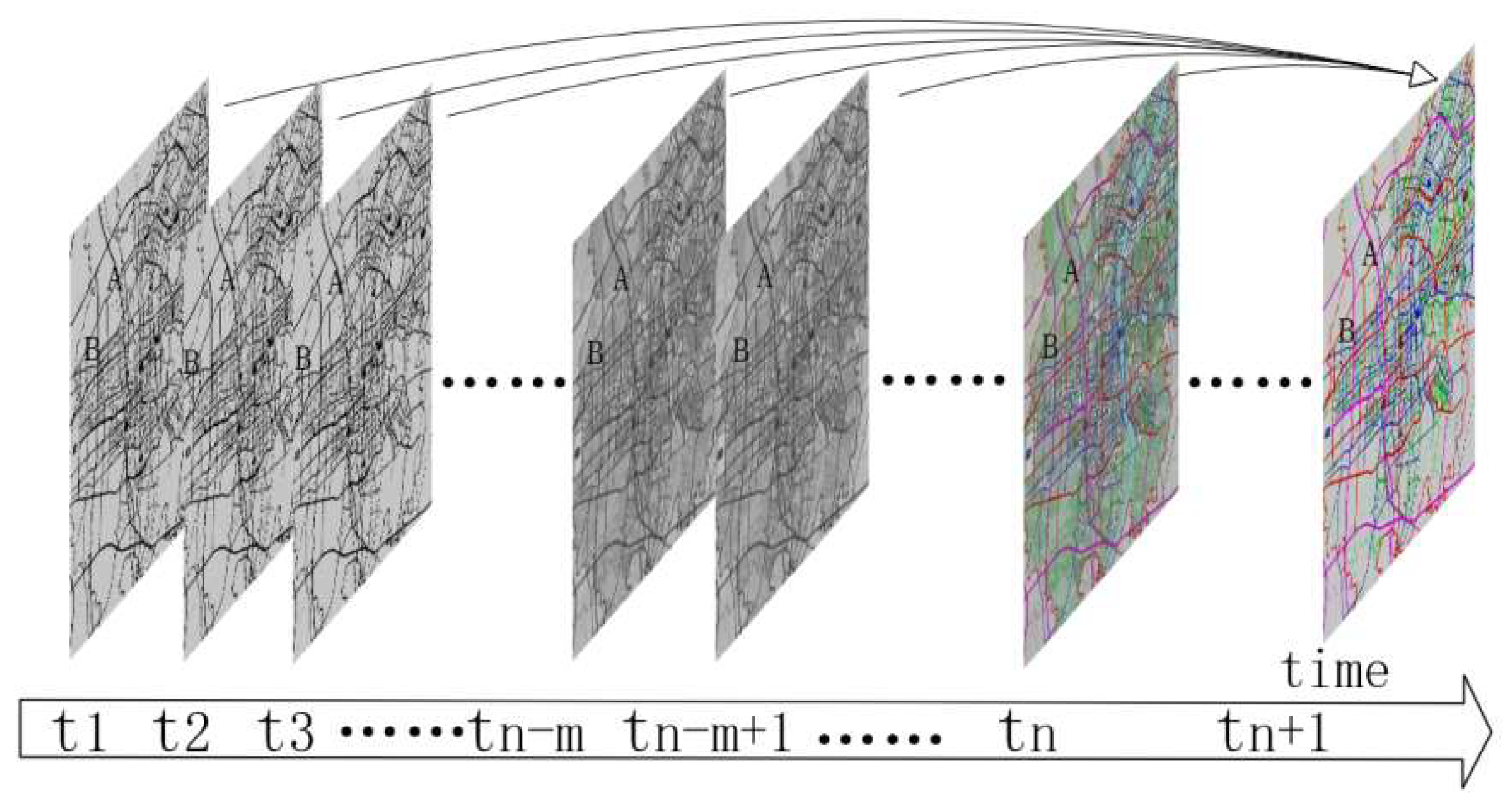
Figure 4.
Sampling of One Day's Data in the PEMS04 Dataset.
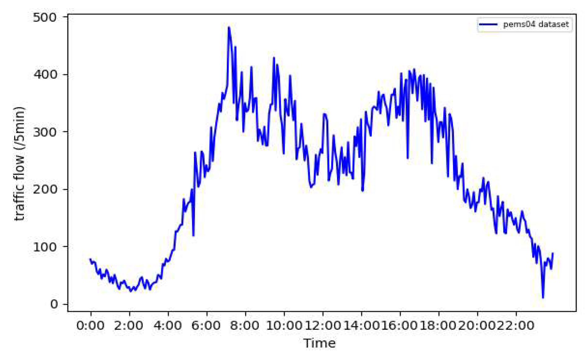
Figure 5.
Sampling of the PEMS04 Dataset.
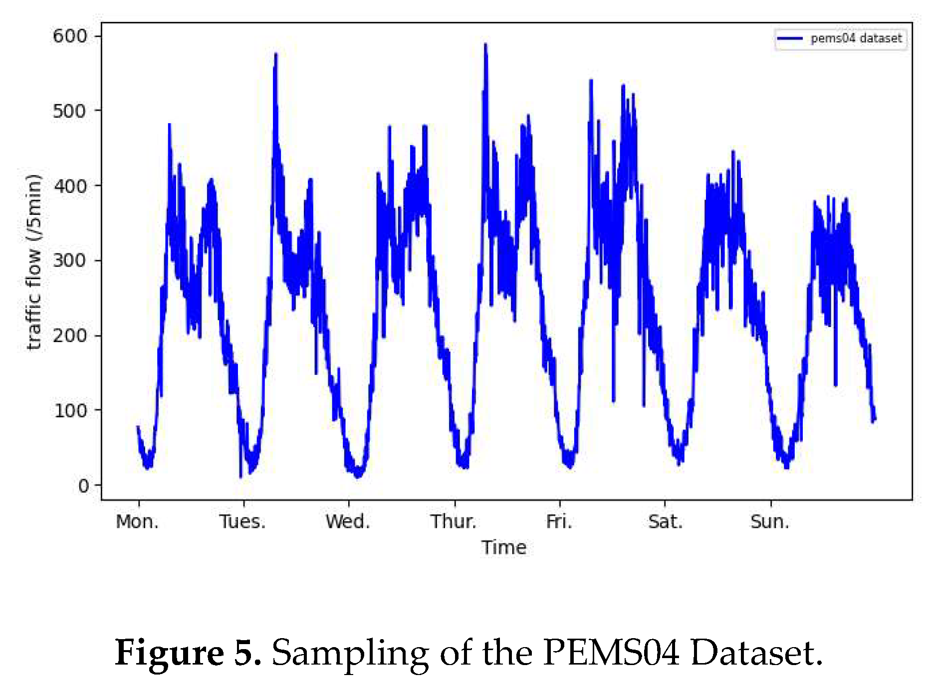
Figure 6.
Calculation Process of the Periodic Difference of the Dataset.
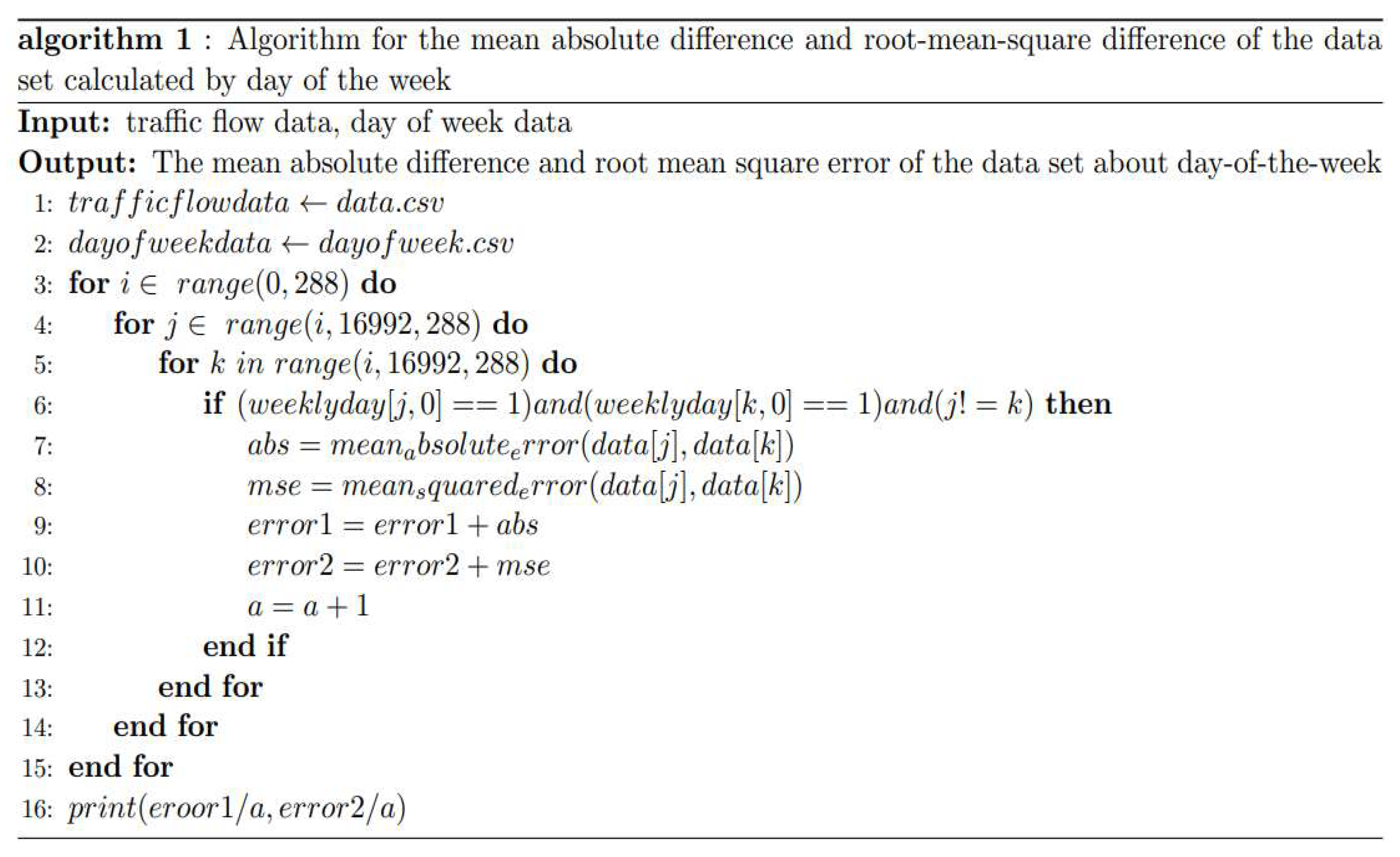
Figure 7.
Schematic diagram of external factor integration.
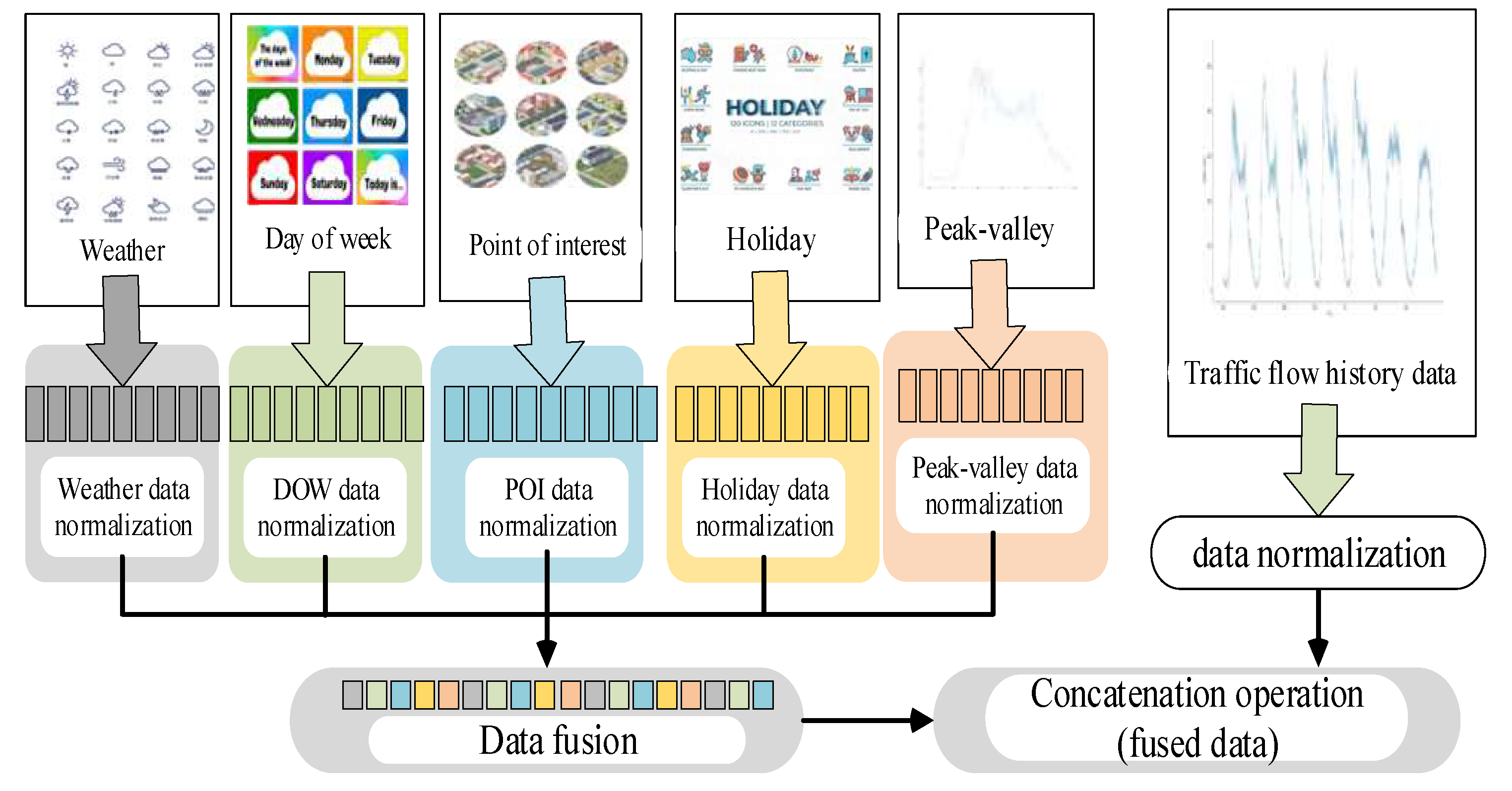
Figure 8.
Pseudo code for the data fusion algorithm of external factors affecting traffic flow.
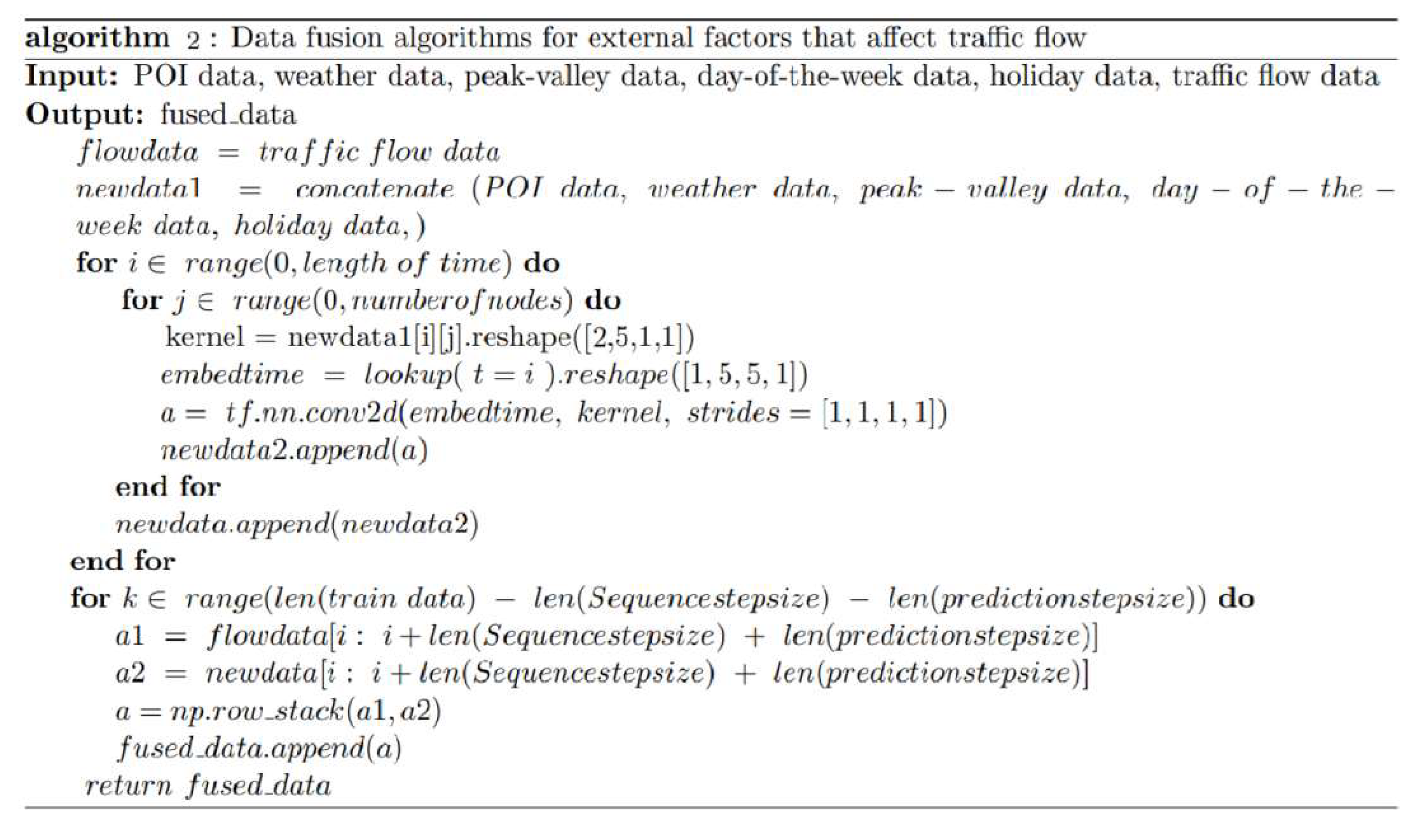
Figure 9.
Process Framework for Integrating External Factors Affecting Traffic Flow.
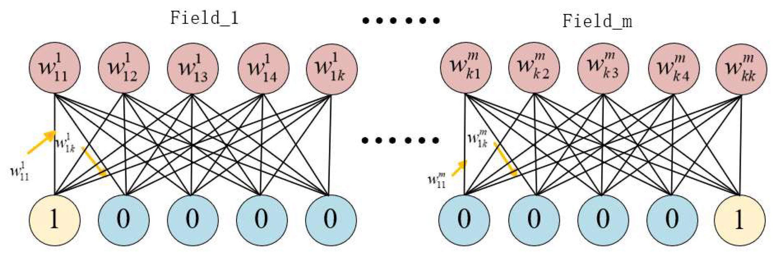
Figure 10.
Schematic Diagram of the lookup Lookup Function.
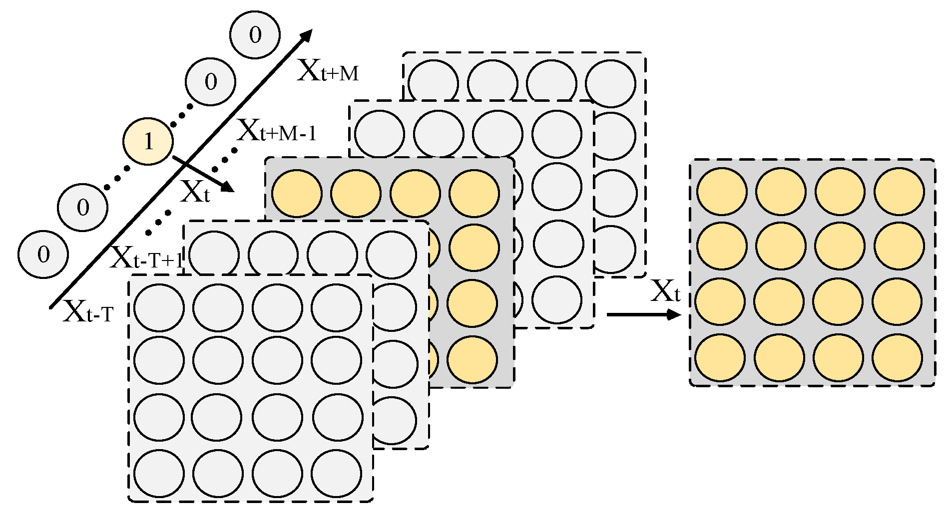
Figure 11.
Overall Framework of the Data Fusion Process.
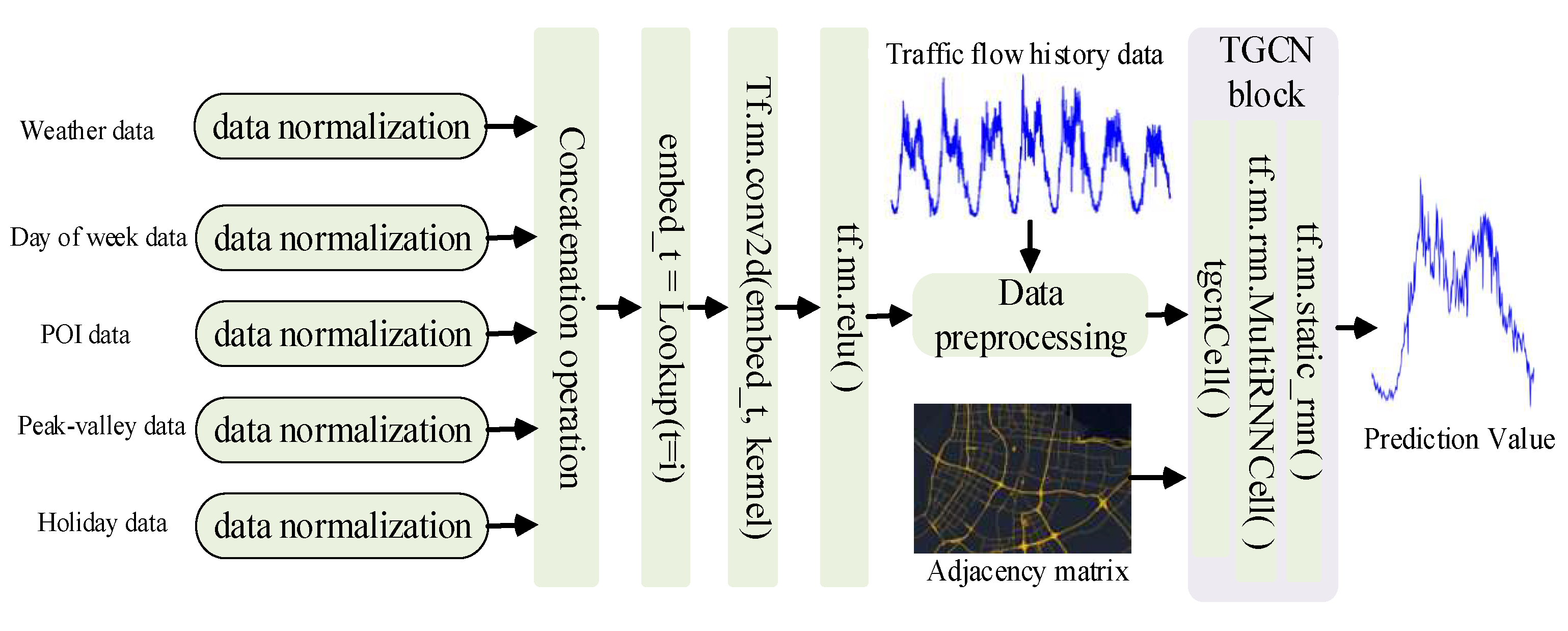
Figure 12.
Test Results of the SZ-taxi Data Set.
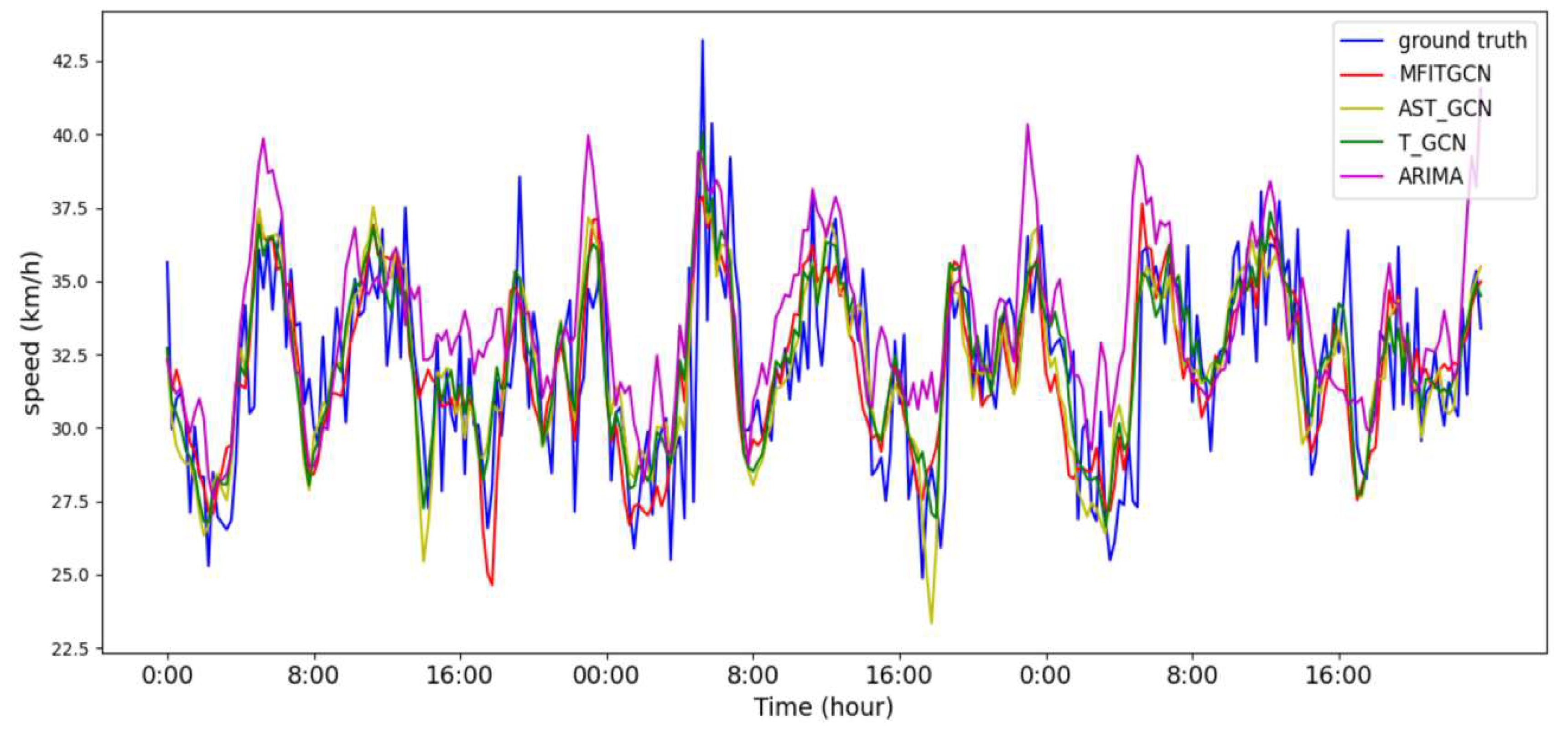
Figure 13.
Test Results of the PEMS04 Data Set.
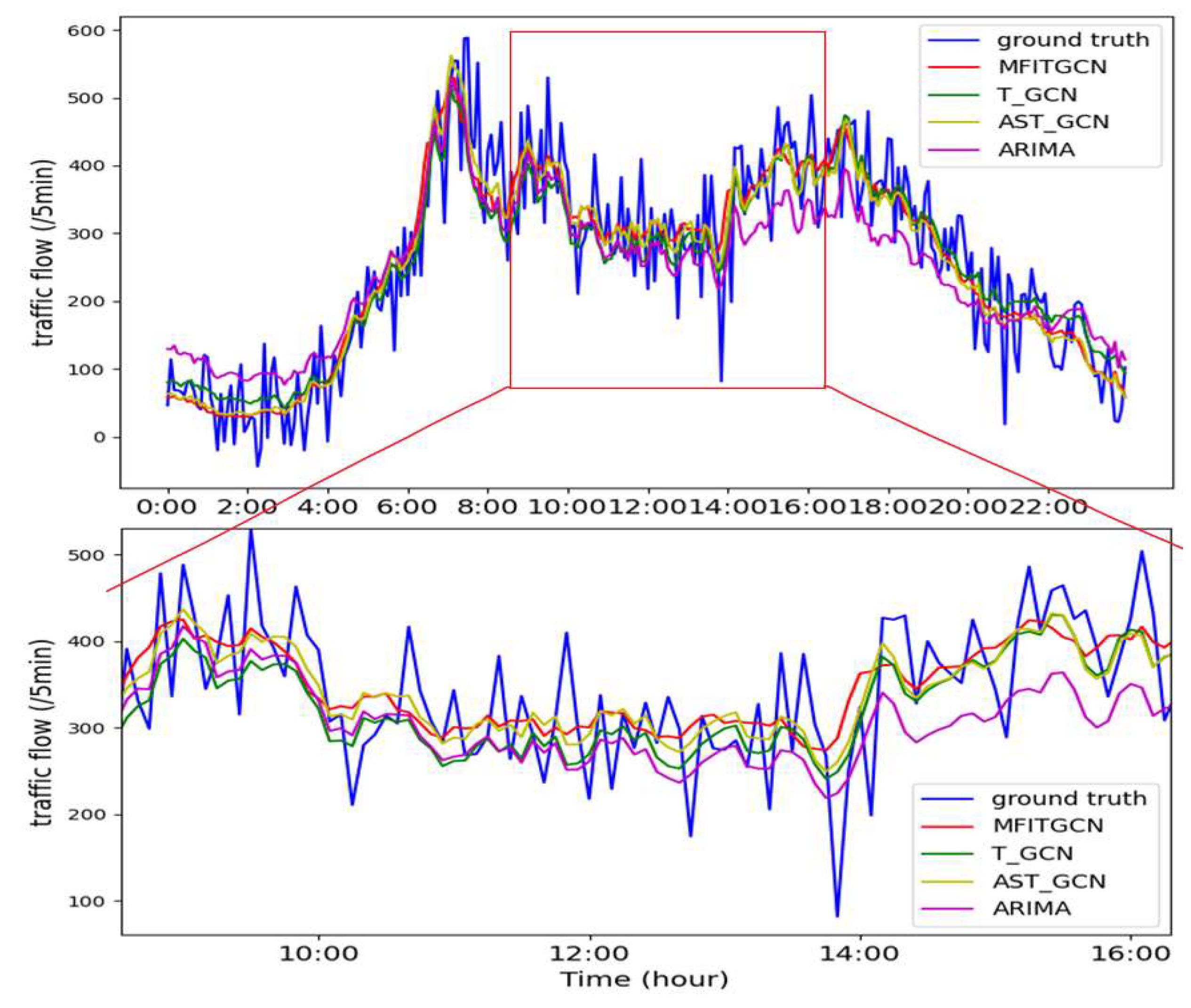
Figure 14.
Ablation Experiments on Various Elements Affecting Traffic Flow.
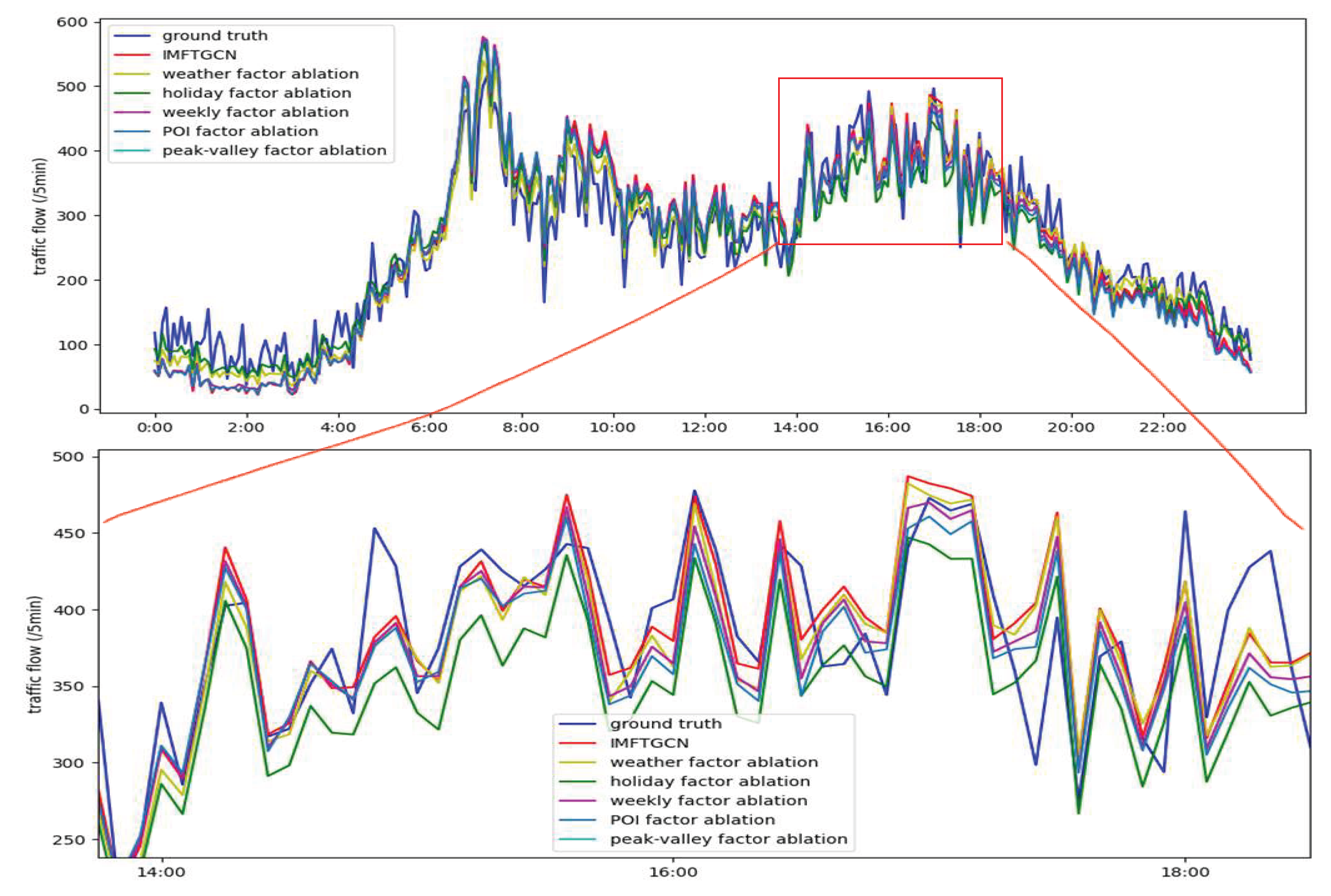

Table 1.
Division of Traffic Flow Peak and Valley Periods in a Day.
| Classification of time period | Tme period |
|---|---|
| Morning traffic period(1) | From 5:00 to 7:00 |
| Morning rush hour.(2) | From 7:00 to 9:00 |
| Day time traffic period(3) | From 9:00 to 17:00 |
| Night rush hour(4) | From 17:00 to 19:00 |
| Night traffic period(5) | From 19:00 to 22:00 |
| Traffic period in the early morning(6) | From 22:00 to 5:00 the next day |
Table 2.
Differences in the PEMS04 data distinguished by the day-of-the-week.
| Differences among data in the data set | Mon. | Tues. | Wed. | Thur. | Fri. | Sat. | Sun. | |
|---|---|---|---|---|---|---|---|---|
| the day-of-the-week (Monday, Tuesday, Wednesday, Thursday, Friday, Saturday, or Sunday respectively) | Mean Absolute Difference | 30 | 30 | 31 | 30 | 31 | 29 | 47 |
| Root Mean Square Deviation | 51 | 47 | 49 | 50 | 50 | 44 | 67 | |
| the other six days of the week excluding the day-of-the-week (Monday, Tuesday, Wednesday, Thursday, Friday, Saturday, or Sunday respectively) | Mean Absolute Difference | 47 | 47 | 46 | 48 | 59 | 68 | 50 |
| Root Mean Square Deviation | 67 | 66 | 66 | 68 | 81 | 90 | 70 | |
Table 3.
Comparison of Performance Metrics among Different Models When Predicting for 15 Minutes Using the SZ-taxi Data Set.
Table 3.
Comparison of Performance Metrics among Different Models When Predicting for 15 Minutes Using the SZ-taxi Data Set.
| Model | RMSE | MAE | ACC | R2 |
|---|---|---|---|---|
| ARIMA | 6.796 | 4.676 | 0.378 | * |
| T-GCN | 4.459 | 2.781 | 0.714 | 0.846 |
| AST-GCN | 4.098 | 2.758 | 0.715 | 0.846 |
| IM-GCN | 3.982 | 2.653 | 0.732 | 0.862 |
Table 4.
Comparison of Performance Metrics among Different Models When Predicting for 5 Minutes Using the PEMS04 Data Set.
Table 4.
Comparison of Performance Metrics among Different Models When Predicting for 5 Minutes Using the PEMS04 Data Set.
| Model | MAE | MAPE(%) | RMSE |
|---|---|---|---|
| LSTM | 29.32 | 15.59 | 45.72 |
| T-GCN | 24.77 | 13.80 | 38.02 |
| AST-GCN | 21.80 | 12.43 | 32.82 |
| IM-GCN | 19.08 | 11.05 | 30.76 |
Table 5.
Comparison of This Model with Models Such as AST-GCN over Multiple Time Steps.
| Time | Model | RMSE | MAE | ACC | R2 |
|---|---|---|---|---|---|
| 15min | TGCN | 4.099 | 2.780 | 0.714 | 0.846 |
| AST-GCN | 4.098 | 2.758 | 0.715 | 0.846 | |
| IM-GCN | 3.882 | 2.683 | 0.732 | 0.858 | |
| 30min | TGCN | 4.151 | 2.820 | 0.711 | 0.842 |
| AST-GCN | 4.147 | 2.815 | 0.712 | 0.843 | |
| IM-GCN | 3.982 | 2.723 | 0.724 | 0.856 | |
| 45min | TGCN | 4.222 | 2.913 | 0.706 | 0.837 |
| AST-GCN | 4.183 | 2.851 | 0.709 | 0.840 | |
| IM-GCN | 4.184 | 2.783 | 0.718 | 0.846 | |
| 60min | TGCN | 4.230 | 2.904 | 0.705 | 0.836 |
| AST-GCN | 4.200 | 2.867 | 0.707 | 0.838 | |
| IM-GCN | 4.202 | 2.781 | 0.713 | 0.842 |
Table 6.
Comparison of Model Performance Metrics in the Ablation Experiment on Factors Affecting Traffic Flow for the PEMS04 Data Set.
Table 6.
Comparison of Model Performance Metrics in the Ablation Experiment on Factors Affecting Traffic Flow for the PEMS04 Data Set.
| Model | MAE | MAPE(%) | RMSE |
|---|---|---|---|
| weather factor ablation | 22.03 | 12.73 | 33.32 |
| holiday factor ablation | 21.66 | 12.52 | 32.14 |
| weekly factor ablation | 21.53 | 12.45 | 32.12 |
| POI factor ablation | 20.49 | 11.84 | 31.87 |
| peak-valley fator ablation | 20.46 | 11.82 | 31.85 |
| IM-GCN | 19.08 | 11.05 | 30.76 |
Table 7.
Record of Time Consumption per Iteration for Each Algorithm Model.
| Model | TGCN | AST-GCN | IM-GCN |
|---|---|---|---|
| Average time consumption per iteration ( s) | 176.6 | 182.5 | 184.2 |
Disclaimer/Publisher’s Note: The statements, opinions and data contained in all publications are solely those of the individual author(s) and contributor(s) and not of MDPI and/or the editor(s). MDPI and/or the editor(s) disclaim responsibility for any injury to people or property resulting from any ideas, methods, instructions or products referred to in the content. |
© 2025 by the authors. Licensee MDPI, Basel, Switzerland. This article is an open access article distributed under the terms and conditions of the Creative Commons Attribution (CC BY) license (http://creativecommons.org/licenses/by/4.0/).
Copyright: This open access article is published under a Creative Commons CC BY 4.0 license, which permit the free download, distribution, and reuse, provided that the author and preprint are cited in any reuse.


