0. Introductory
At 00:03:09 Beijing Time on June 10, 2022, an Ms5.8 earthquake occurred in Maerkang City, Aba Tibetan and Qiang Autonomous Prefecture, Sichuan Province (32.27°N, 101.82°E), with a focal depth of 10 km. After 1 hour, 25 minutes, and 45 seconds, another earthquake of Ms6.0 struck the same area (32.25°N, 101.82°E) at a focal depth of 13 km, with an epicentral distance of only 2.6 km from the first event. After an additional interval of 1 hour, 58 minutes, and 26 seconds, a third earthquake of Ms5.2 occurred (32.24°N, 101.85°E) with a focal depth of 15 km[
1]. As of 23:59 on June 14, a total of 2267 earthquakes had been recorded in the Maerkang region, including one Ms6.0 earthquake, two earthquakes of magnitude 5.0–5.9, four earthquakes of magnitude 4.0–4.9, seven earthquakes of magnitude 3.0–3.9, and 2253 earthquakes below magnitude 3. Hereafter, this sequence of earthquakes is referred to as the “Maerkang Ms6.0 earthquake swarm.” The earthquakes and their induced secondary disasters affected Maerkang City and surrounding areas, causing incalculable casualties and property losses[
2].
Landslide susceptibility assessment involves analyzing evaluation factors using predictive models to derive susceptibility values for evaluation units, which are then classified to obtain landslide susceptibility zoning[
3]. This process emphasizes the relationship between historical landslide disasters and various influencing factors such as geology, topography, geomorphology, soil characteristics, and human activities, with the goal of estimating the likelihood of landslides in specific areas[
4,
5]. In recent years, geological disasters have caused increasing losses to society, making the accurate assessment of landslide susceptibility an important research task. At present, statistical analysis-based methods have become the mainstream approach for landslide susceptibility assessment, which can be broadly categorized into classical statistical methods and machine learning (ML)-based methods. Traditional statistical models can effectively reflect the development patterns of landslides when applied to susceptibility assessment. However, they tend to overestimate the extent of high and very high susceptibility zones, resulting in low prediction efficiency. In contrast, ML models exhibit higher accuracy and practical applicability but suffer from a lack of guidance in non-sample selection and are prone to overfitting when input features correspond directly to evaluation factor attributes. Moreover, the reliability and accuracy of single-model predictions are difficult to ensure in regions with complex geological and geomorphological conditions[
6,
7].
In this study, the Information Value-Analytic Hierarchy Process (IV-AHP) model was selected as a representative of traditional statistical analysis methods, while the Random Forest (RF) and Extreme Gradient Boosting (XGBoost) models were chosen as representatives of tree-based ML models. Furthermore, IV-RF and IV-XGBoost hybrid models were introduced to integrate the advantages of statistical analysis and machine learning approaches. Given the complex natural geographic conditions of the study area, twelve evaluation factors—terrain relief, slope, curvature, rock hardness, NDVI, TWI, SPI, PGA, distance to roads, distance to water systems, distance to faults, and land use type—were selected as indicators for assessing landslide susceptibility in the study area[
8,
9,
10]. The study then predicted the spatial distribution probability of landslides induced by the Maerkang Ms6.0 earthquake swarm to achieve a more accurate evaluation of regional landslide susceptibility. Additionally, the accuracy of the five models was compared, and the strengths and weaknesses of machine learning and traditional statistical methods were further explored.
1. Overview of the Study Area
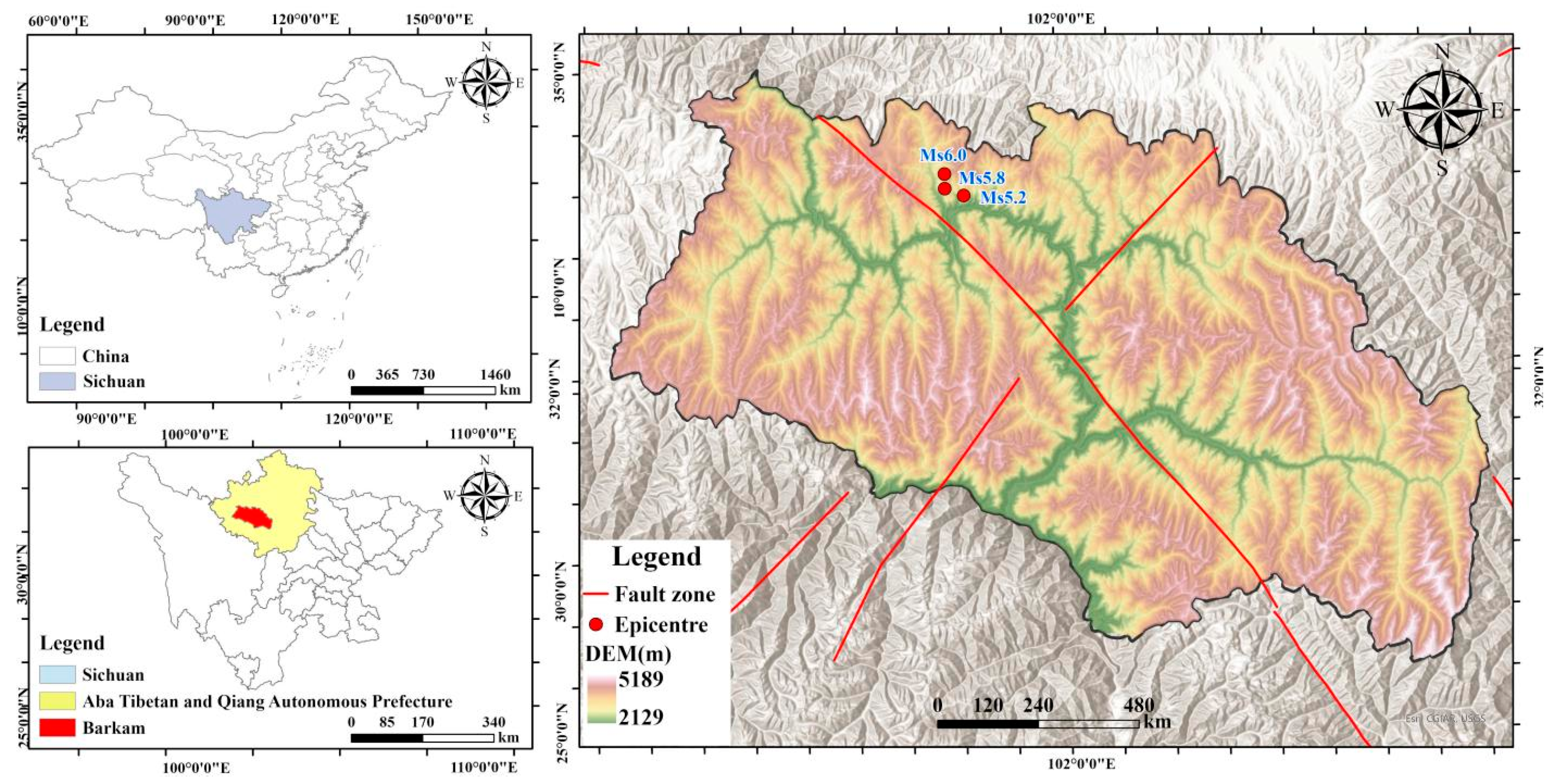
Maerkang City is located at the southern end of the northwestern Sichuan Plateau and belongs to the plateau canyon region. The terrain is an irregular rectangle, gradually decreasing in elevation from northeast to southwest (
Figure 1).
The area is characterized by continuous mountain ranges and steep valleys, with a complex geological structure dominated by Triassic formations, including sandstone, slate, and metamorphic rocks. The average elevation of Maerkang City exceeds 3000 m, with the overall landscape forming a typical plateau characterized by high terrain, consisting of hummocky plateau surfaces and dissected mountain summits. The mountains are higher in the south and lower in the north, while river valleys exhibit a northwest-to-southeast gradient. The primary mountain and river orientations follow a northwest-southeast trend.
The earthquake sequence occurred at the junction of the southern segment of the Longriba Fault and the Songgang Fault, within the Bayan Har Block, a region with relatively complex tectonics. The area is characterized by rugged mountains with significant elevation differences between ridges and valleys, reaching 1800–2300 m. More than 40 anticlines are distributed within the region, with frequent occurrences of structural compounding, making it an area of active moderate to small earthquakes. The Songgang Fault Zone trends approximately northwest[
11], with the Bayan Har Block bordered by the Longriba Fault Zone (
Figure 1). To the east lies the secondary Longmenshan Block, consisting of the Changan Fault, Loucun Fault, and Jinsha Fault. This fault system originates on the northern slopes of Mengbi Mountain, south of Maerkang, extends northwestward along the Jiamuzu River after intersecting the Songgang Fault, and continues through the regions of Dalcang and Ruo’ergai. The area exhibits intense tectonic uplift, deeply incised river valleys, significant topographic relief, diverse landform types, and well-developed active faults[
12,
13,
14]
.
According to the landslide inventory interpreted after the earthquake, the seismic swarm induced a total of 1142 landslides, including 891 small-scale landslides, 242 medium-scale landslides, 9 large-scale landslides, and no extremely large landslides. Most of these were soil landslides, with landslide materials primarily consisting of silty clay, blocky gravel soil, and gravel soil.
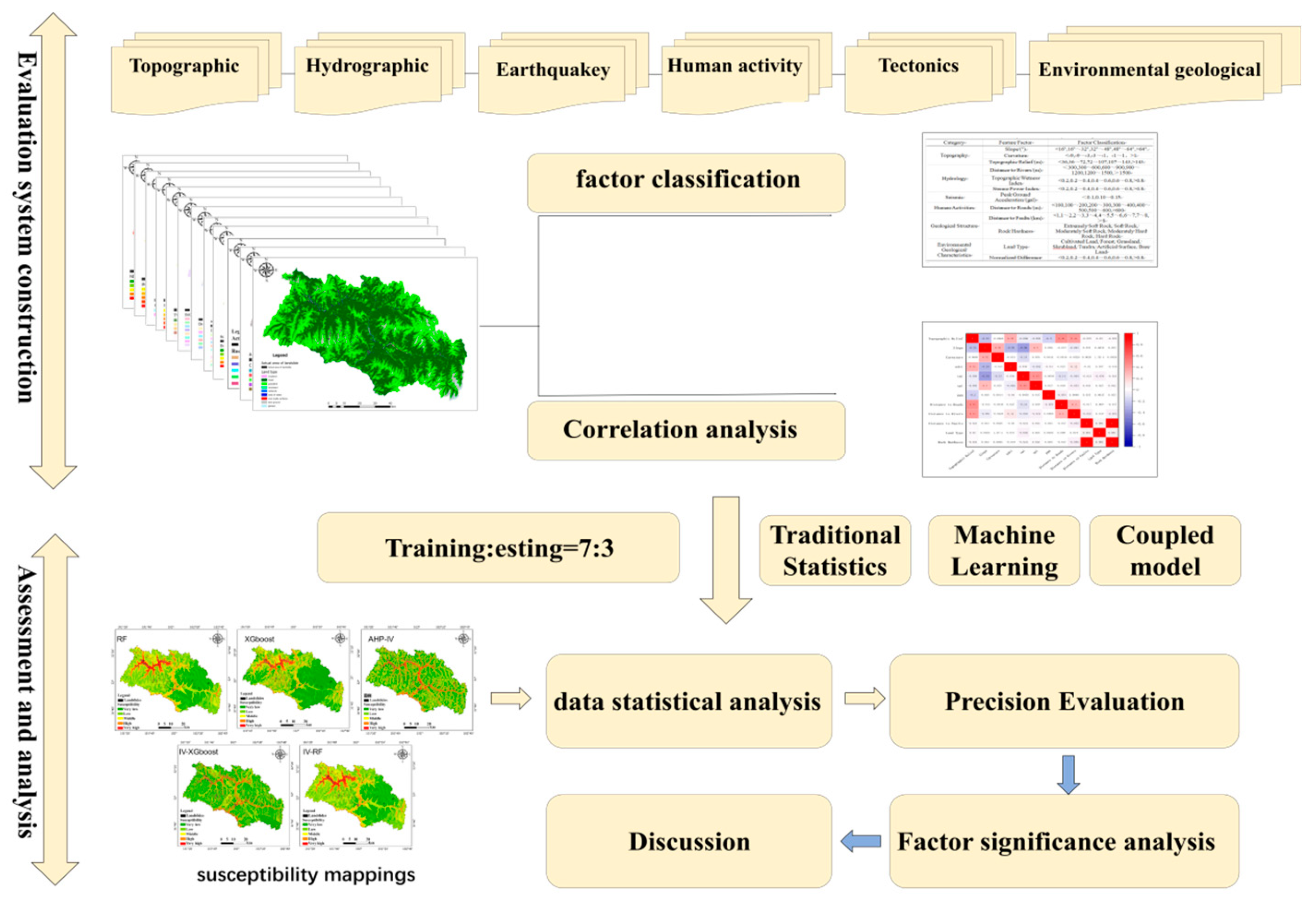
2. Data and Methods
This study aims to assess the landslide susceptibility of Maerkang City using the RF, XGBoost, IV-AHP, IV-RF, and IV-XGBoost models. By conducting a comparative analysis of the strengths and weaknesses of machine learning methods and traditional statistical analysis methods, the study seeks to develop hybrid models to further enhance prediction accuracy. The specific workflow is illustrated in
Figure 2.
2.1. Data
Domestic and international studies on the influencing factors and factor selection of earthquake-induced landslides have been extensive, mainly focusing on the combined effects of seismic action, topography, geological structure, and hydrological conditions, with indicator selection also revolving around these four aspects[
15,
16,
17].
Based on the disaster-pregnant conditions of landslides, 12 evaluation factors were selected from six aspects: topography, earthquake, hydrology, human activities, geological structure, and environmental geological characteristics, as shown in
Table 1.
(1) Topographic data: Based on the study area’s DEM data with a spatial resolution of 12.5m, topographic relief, slope, and curvature were extracted using ArcGIS.
(2) Hydrological data: The study area’s SPI and TWI were obtained through hydrological processing of the 12.5m DEM data using ArcGIS, and the distance to rivers was obtained by processing river data using the “multi-ring buffer” function.
(3) Seismic data: The PGA vector data for the study area was obtained by clipping the peak ground acceleration of this earthquake (released by the China Earthquake Networks Center) using ArcGIS.
(4) Human activities: Road data for the study area was extracted from 1:250,000 basic geographic information data, and the distance to roads was obtained by processing road data using the “multi-ring buffer” function.
(5) Geological structure: Fault zone data and stratum rock data for the study area were obtained from the Resource and Environment Science and Data Center of the Chinese Academy of Sciences (
http://www.resdc.cn/), and the distance to fault zones was obtained after coordinate conversion. The rock hardness was classified according to the qualitative classification standard table for rock hardness levels.
(6) Vegetation coverage data: The NDVI for the study area was calculated using the near-infrared and far-infrared bands of Landsat8 with a resolution of 30m from August 2022, when vegetation was most abundant. The land use type vector data for the study area was obtained by clipping global 30m land cover data (
http://www.globeland30.org/home/background.aspx)。
Figure 3.
Characteristic factor map.
Figure 3.
Characteristic factor map.
2.2. Research Methods
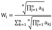
2.2.1. Information Value-Analytic Hierarchy Process (IV-AHP)
Integrating the Analytic Hierarchy Process (AHP) with the Information Value (IV) model has become a well-established approach in recent years. This method effectively addresses the subjectivity inherent in expert judgment while mitigating the uncertainties caused by data noise in the IV model. As a result, it provides a more reliable framework for analyzing coseismic landslide susceptibility.
In the IV model, the information value
for a specific evaluation factor
is calculated as follows:
where: S represents the total number of evaluation units in the study area;
is the number of units containing the evaluation factor
; N denotes the total number of units in the study area where landslides have occurred;
is the number of landslide-affected units within a specific category of factor
.
After obtaining the information value
for each factor using the IV model, AHP is applied to compute the weight
of each factor. The weighted total information value is then derived by summing the products of each factor’s information value and its corresponding weight[
18,
19]. Landslide susceptibility zones are classified based on the magnitude of the weighted total information value, calculated as follows:
where:
represents the total information value of an evaluation unit;
is the weight assigned to the
factor;
is the information value of the
factor.
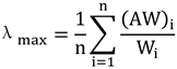
In the AHP method, a judgment matrix is constructed, where represents the relative importance of factor compared to factor . Typically, a 1 – 9 scale is used to assign values. After constructing the judgment matrix, the square root method is employed to compute the maximum eigenvalue and the corresponding eigenvector.
The eigenvector
, which represents the initial weights of the factors, is calculated as follows:
where each component
corresponds to the initial weight of the respective factor. Subsequently, the maximum eigenvalue
is computed using:
where
represents the
component of the vector
.
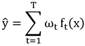
2.2.2. Extreme Gradient Boosting (XGBoost)
XGBoost is an extension of the Gradient Boosting Decision Tree (GBDT) that incorporates regularization (L1, L2) to prevent overfitting, supports parallel computation for enhanced efficiency, handles missing values, and provides feature importance scores. The model fits the residuals between the predicted values from the previous decision tree and the actual observed values. Through multiple iterations, the residuals are approximated to the observed values, and the prediction results from multiple decision trees are weighted and summed to obtain the final[
18,
19] prediction. Assuming
decision trees are trained,
represents the prediction result of the
decision tree for sample
, and
represents the weight of the
decision tree, the final prediction
from the XGBoost model for sample
is calculated as:
In XGBoost’s practical application, the model learns the structure of each decision tree (i.e., the specific form of ) and their corresponding weights . During the prediction phase, the sample is input into each decision tree, and the corresponding prediction results are aggregated using the learned weights to obtain the final prediction value . In the landslide susceptibility assessment, the predicted value represents the landslide susceptibility score for the region where the sample is located.
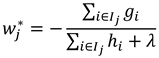
In susceptibility evaluation, XGBoost takes input features, learns their relationship with disaster occurrence, and outputs a susceptibility score. By initializing the model, optimizing iteratively, and controlling regularization, it generates a high-precision prediction model suitable for modeling complex nonlinear relationships. The optimal weight at the leaf node is the weight corresponding to the leaf node that minimizes the objective function. The optimal weight
calculation is as follows:
where
and
are the first and second derivatives of the loss function, respectively;
is the sample set belonging to the
leaf node;
is the regularization parameter.
XGBoost minimizes the loss function iteratively by adding tree models and introduces a regularization term to control the complexity of the model. The composite objective function that integrates loss and model complexity is given by:
where:
and
are the accumulated first and second derivatives of the samples in the
leaf node;
is the weight of the
leaf node;
and
are regularization parameters that control the model’s complexity.
2.2.3. Random Forest (RF)
Random Forest (RF) is an ensemble learning algorithm that constructs multiple decision trees and combines their prediction results to improve overall accuracy. It randomly selects several subsets from the original dataset as training sets. For each training set, a decision tree is built using a random subset of features. This process helps reduce overfitting. Each decision tree is trained using its corresponding training set until a stopping criterion is met.
During the training process of the random forest, due to the random subset selection for each decision tree, some data are not used for training a particular decision tree. These data are referred to as out-of-bag (OOB) data. The OOB error is used to assess the model’s performance[
21,
22]. The OOB error is calculated as:
where:
is the total number of samples;
indicates whether the prediction for the
sample using decision trees trained without that sample is correct (if the prediction is correct,
; if the prediction is incorrect,
).
By calculating the OOB error, the generalization ability of the random forest model can be evaluated without additional cross-validation. A lower OOB error suggests better model performance. When predicting new data, the final prediction is determined by combining the training results from each decision tree through voting or averaging, in line with the Bagging ensemble concept.
2.2.4. IV-XGBoost and IV-RF Coupling Models
The coupling models primarily utilize the IV model to integrate data from different factors and their classifications, compensating for the blind selection of non-landslide samples in RF or XGBoost models. These models can uncover hidden patterns in the data. The coupling process is reflected in two aspects: Random selection of non-landslide samples from the very low or low susceptibility areas in the IV model; Inputting the information value processed by the IV model into the data of RF or XGBoost. By using the information value, the models effectively reduce feature redundancy, significantly enhancing both model performance and interpretability[
23].
2.2.5. Model Accuracy Evaluation
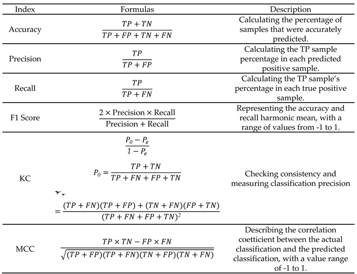
(1)Accuracy, precision, recall , F1 score, KC and MCC
An important part of landslide susceptibility assessment is model validation and performance evaluation. Typically, the performance of binary classification models is assessed using a confusion matrix. The confusion matrix consists of four parameters: True Positive (TP) represents the number of instances where the model predicts a landslide and the actual event is a landslide; False Negative (FN) represents the number of instances where the model predicts a non-landslide but the actual event is a landslide; False Positive (FP) represents the number of instances where the model predicts a landslide but the actual event is a non-landslide; True Negative (TN) represents the number of instances where the model predicts a non-landslide and the actual event is a non-landslide[
24]. Based on these parameters, the performance of each model is evaluated using six statistical indicators: accuracy, precision, recall, F1 score, Kappa coefficient (KC), and Matthew’s correlation coefficient (MCC).
Table 2 presents the description of each indicator.
(2)ROC values and AUC curves
The True Positive Rate (TPR) is shown on the vertical axis of the Receiver Operating Characteristic (ROC) curve, and the False Positive Rate (FPR) is shown on the horizontal axis. It displays how well the model performs at various classification thresholds. The percentage of negative samples that are mis predicted as positive is known as the False Positive Rate, whereas the percentage of positive samples that are accurately predicted as positive is known as the True Positive Rate. The model performs better the closer the ROC curve is to the upper left corner. The Area Under the Curve (AUC), which offers a thorough assessment of the model’s performance, is the area under the ROC curve. The model’s predictive performance is equal to random guessing when the AUC value is zero. The model is said to be fully capable of differentiating between positive and negative samples when the AUC value is 1. The predictive performance of the model is better when the AUC value is near 1[
25].
2.2.6. Comprehensive Comparative Analysis
To comprehensively evaluate the performance of each model, this study conducted a systematic and comprehensive comparison. In terms of accuracy evaluation, in addition to calculating the common indicators mentioned above, multiple rounds of cross-validation were also performed. The dataset was randomly divided into multiple subsets, with each subset selected as the test set while the remaining data was used as the training set. This process was repeated multiple times, and the accuracy indicators of each model were calculated for different data splits and averaged. This effectively reduced the impact of dataset partitioning differences on the evaluation results, making the accuracy evaluation more reliable.
In the result evaluation comparison, not only were the predicted landslide susceptibility class distributions of each model compared, but the prediction differences for the same region were also analyzed in depth. For high-susceptibility areas, special attention was paid to the number of landslides predicted by each model and their distribution density; for low-susceptibility areas, the focus was on the stability of model predictions. At the same time, by combining the actual geological, topographical conditions and historical landslide data of the study area, the rationality of the model’s predictions was assessed. The onsite landslide survey data was analyzed to determine whether the model could accurately reflect the high landslide risk characteristics of regions with complex geological structures and steep terrain, and whether the low-risk predictions in areas with flat terrain and stable geological conditions were reasonable. Through this comprehensive comparison, a deeper understanding of the strengths and weaknesses of each model can be gained, providing strong evidence for model selection and optimization.
3. Results and Analysis
3.1. Selection and Construction of the Indicator System
This study identifies the primary factors controlling the occurrence of co-seismic landslide disasters as both background and external conditions. Background conditions refer to the fundamental factors that influence the occurrence of co-seismic landslides, including topography and landforms, geological structures, hydrogeology, and stratigraphy. External conditions refer to the triggering factors that cause co-seismic landslides, mainly including earthquake intensity and human engineering activities. Based on this selection rationale, the study chooses 12 key factors for the co-seismic landslide susceptibility assessment system, including slope, vegetation cover index (NDVI), peak ground acceleration (PGA), stream power index (SPI), topographic wetness index (TWI), distance to roads, distance to faults, distance to rivers, topographic relief, curvature, land type, and rock hardness[
26,
27]
. These factors are then classified according to the actual conditions (
Table 3).
This study constructs a hierarchical model to decompose complex issues into factors at different levels. For the factors at the same level, pairwise comparisons are used to construct a judgment matrix. The principal eigenvalue and eigenvector of the judgment matrix are calculated using the square root method, which leads to the initial weights of the factors. After performing a consistency check to ensure the rationality of the judgment matrix, the final weights of the factors are determined. The constructed judgment matrix is shown in the
Table 4.
Through consistency judgment, the results show that λ_max is 14.3241 and the consistency ratio is 0.0707. This proves that the weights are valid and meet the consistency check requirements.
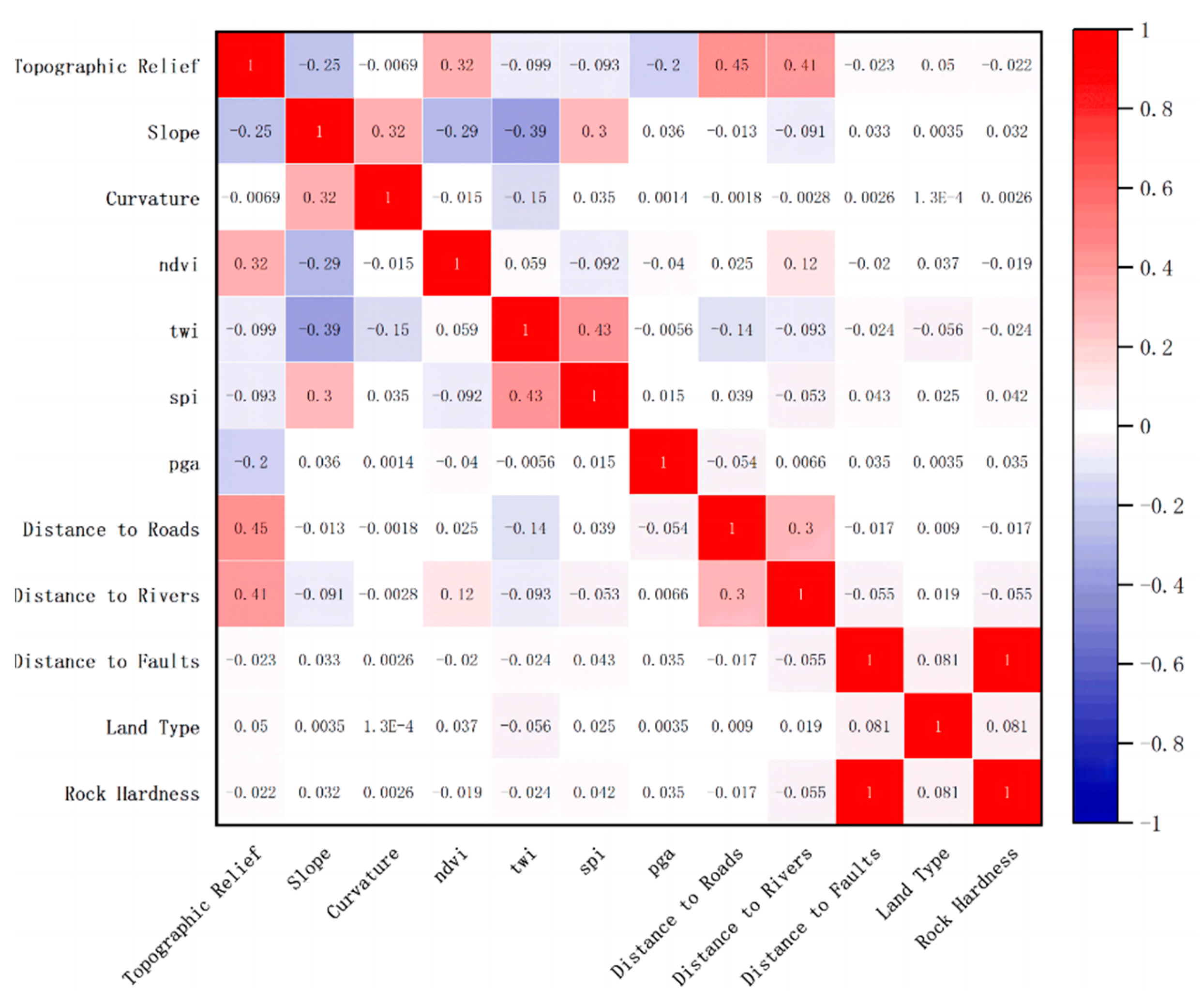
A correlation analysis was conducted on the 12 selected evaluation indicators to identify the most predictive factors and improve the model’s prediction accuracy. Using the Correlation Plot plugin of Origin drawing software, a correlation matrix for the 12 evaluation indicators was created (
Figure 4). Red represents positive correlation, while blue represents negative correlation. The intensity of the colors is directly related to the magnitude of the correlation coefficient. From the figure, it can be observed that all the correlation coefficients of the evaluation factors are below 0.45, indicating a relatively weak correlation. This suggests that the interaction between the factors is minimal, and the selected evaluation factors are reasonable for the model.
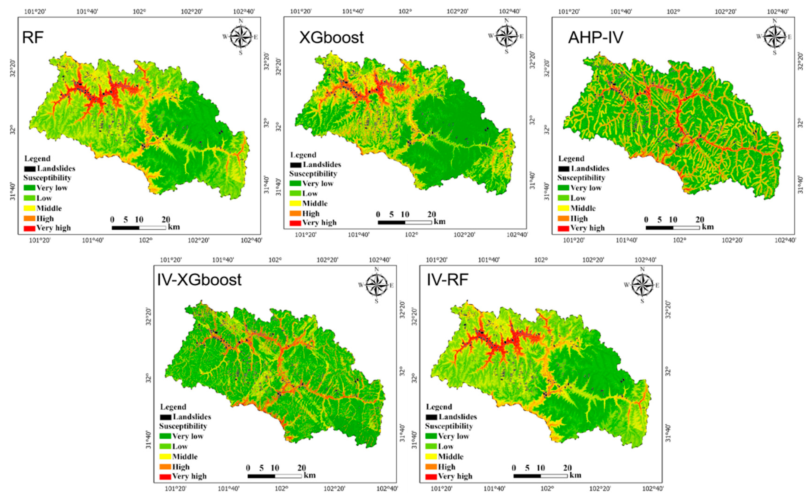
3.2. Analysis of Susceptibility Results
Based on the processed evaluation factors and relevant vector data obtained from the landslide point catalog and field investigations, 1,142 landslide points were obtained using the spatial join tool in ArcGIS. A total of 1,142 non-landslide points were generated, forming a landslide-non-landslide dataset. 70% of the sample set was used for model training, and the remaining 30% was used for model testing[
28]. The trained RF, XGBoost, IV-RF, IV-XGBoost, and IV-AHP models were used to predict the landslide susceptibility values. The final landslide susceptibility value range was [0,1]. The natural breaks method was applied to classify the landslide susceptibility index, resulting in regional landslide susceptibility evaluation maps for the five models, as shown in
Figure 5.
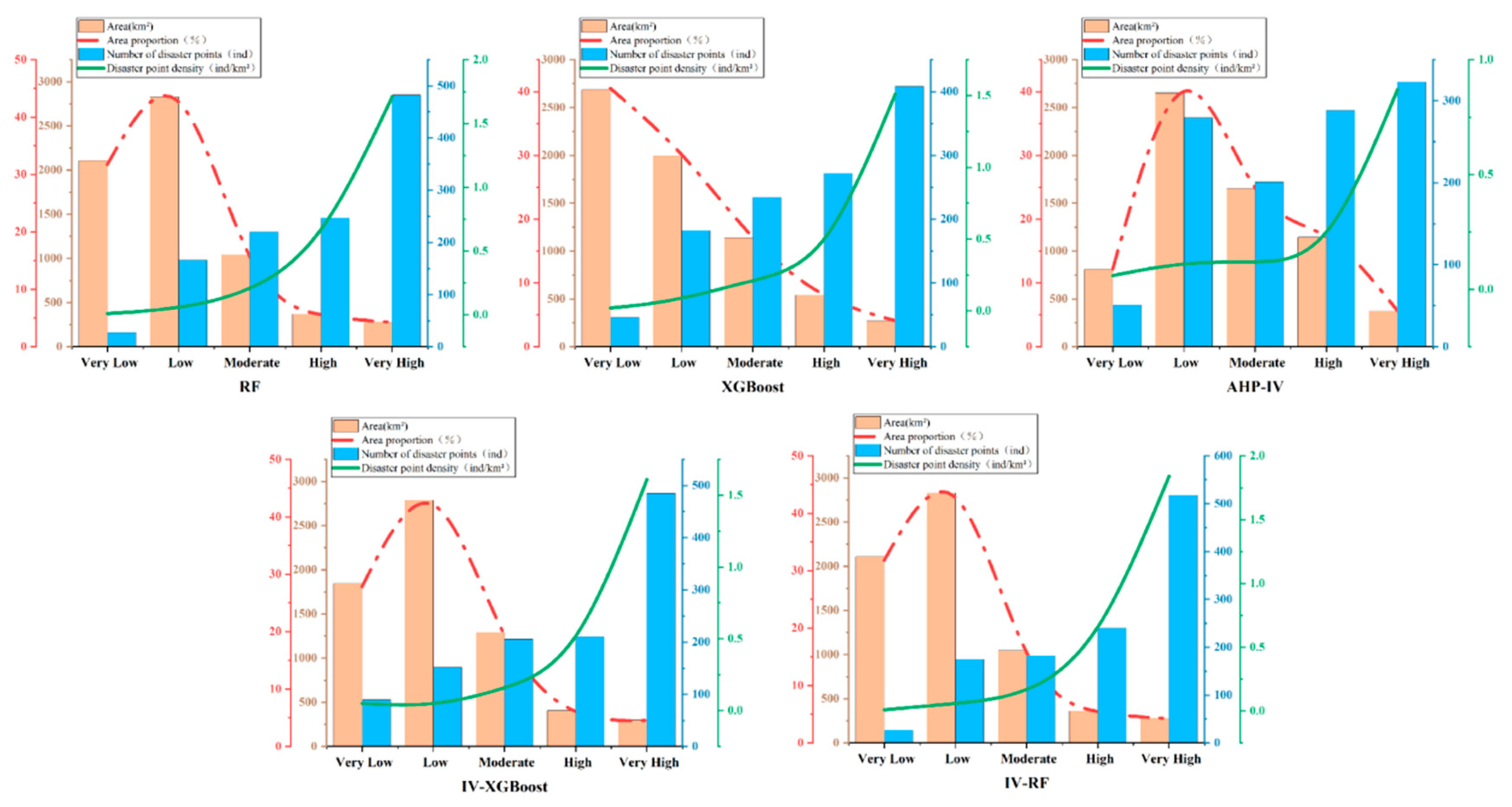
From
Table 5 and
Figure 6, it is evident that compared to traditional statistical analysis methods, the predictive accuracy of machine learning methods is relatively higher. This is mainly reflected in two aspects: first, the number of landslides predicted in the extremely high and high susceptibility zones is higher in the two machine learning models than in the information-based AHP model. In terms of disaster density, the information-based AHP model predicts a disaster density of 0.87 incidents/km², while the XGBoost and RF models predict disaster densities of 1.51 incidents/km² and 1.71 incidents/km², respectively. This indicates that machine learning algorithms provide predictions that are closer to the actual situation than traditional statistical methods.
When comparing the coupled models with machine learning models, the IV-XGBoost and IV-RF coupled models predict significantly more landslides in the high and extremely high susceptibility zones compared to XGBoost and RF models. The landslides predicted in the extremely high and high susceptibility zones by IV-XGBoost account for 60.86% of the total landslides, and by IV-RF, they account for 66.38% of the total. In comparison, the landslides predicted in these zones by XGBoost and RF account for 59.55% and 63.84%, respectively. This shows that the coupled models exhibit better predictive ability in high-risk areas.
In terms of disaster density, the coupled models show higher disaster densities in the extremely high and high susceptibility areas compared to machine learning models, indicating that the predictive accuracy of the coupled models is higher in these high-risk zones. However, in lower susceptibility areas, the IV-XGBoost model predicts a disaster density of 0.05 incidents/km², while the XGBoost model predicts a disaster density of 0.02 incidents/km². This discrepancy may be due to overestimating landslides in the extremely low and low susceptibility zones during the calculation, leading to an overprediction or misclassification.
Overall, machine learning models show more conservative predictions in low susceptibility areas, which reflects their more robust performance, making them better suited for accurate predictions in low-risk areas. In contrast, the coupled models further improve predictive accuracy, making them more accurate and intuitive for predicting landslides in high-risk areas, which is more aligned with disaster prediction needs.
3.3. Model Accuracy Validation
The five landslide susceptibility assessment models used in this study were trained and tested using a single dataset, with 70% of the data used for training and 30% for testing. Model performance metrics, including accuracy, precision, recall, F1 score, KC, MCC, and values of TP, FN, FP, and TN, were calculated (
Table 6).
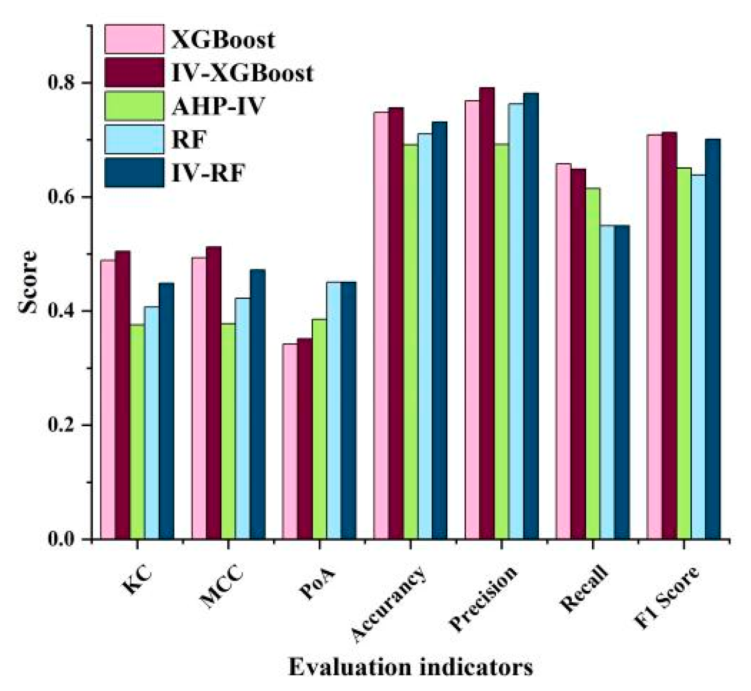
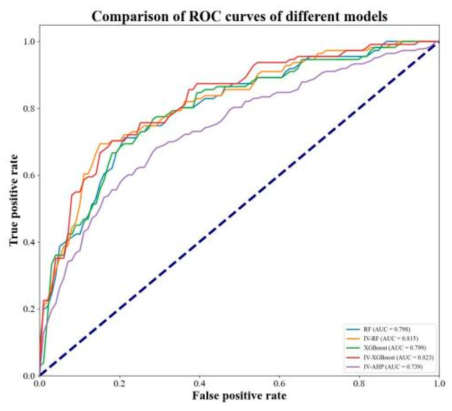
Figure 8 displays the ROC curves of the five models for landslide susceptibility assessment. The ROC curve is generated by progressively lowering the landslide susceptibility threshold and obtaining the coordinates of the corresponding points on the curve. The closer the curve is to the upper left corner, the more landslides are concentrated in areas with higher risk and narrower ranges, leading to a larger AUC value and better predictive performance. In this study, the AUC value of the IV-AHP model was 0.739, lower than the AUC values of the RF and XGBoost models, which were 0.798 and 0.799, respectively. In contrast, the coupled models IV-RF and IV-XGBoost achieved AUC values of 0.815 and 0.823. Overall, from the landslide susceptibility evaluation across the five models, the coupled models performed the best.
Figure 7.
Statistics of model performance metric.
Figure 7.
Statistics of model performance metric.
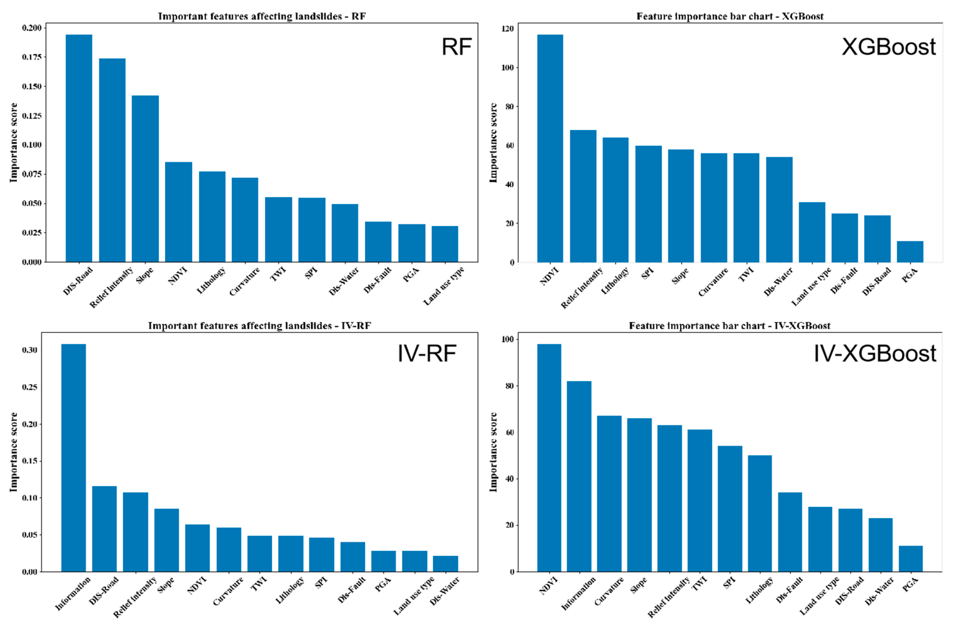
3.4. Factor Significance Analysis
Effective landslide disaster prevention and mitigation strategies depend on identifying the key disaster-causing factors, which may be caused by many interrelated and complex factors. In this susceptibility assessment, the IV-AHP model, Random Forest model, XGBoost model, IV-XGBoost model, and IV-RF model were used. The factor importance for the IV-AHP model was calculated using statistical methods (
Table 3). This process integrates expert knowledge and subjective judgment to determine the importance of evaluation factors in susceptibility assessment, reflecting pure subjectivity.
On the other hand, machine learning models rely on machines to automatically mine the underlying relationships between features and outcomes based on large amounts of data, and then calculate factor importance. Different machine learning models and coupled models have distinct characteristics in terms of calculation logic and data processing methods, which leads to some differences in the ranking of factor importance. These differences reflect the models’ varying understanding of the role of different factors and provide a multidimensional perspective for in-depth analysis of susceptibility influencing factors.
The 12 selected influencing factors in this study have varying degrees of impact on landslide occurrence. Based on the machine learning models, the information value was calculated and used as evaluation factors to form coupled models. The importance analysis of the factors for machine learning models and coupled models is shown in
Figure 9, where shown that the importance scores and rankings of the different factors vary greatly in each model. RF and XGBoost assess feature importance based on their unique algorithms, while IV-RF and IV-XGBoost, combined with information value optimization, select features with better discriminative power. These differences reflect the comprehensive influence of model principles, data characteristics, and parameter settings.
4. Discussions
Based on the comparison of evaluation results, the coupled model demonstrates superior speed and accuracy compared to the traditional Information Value method and standalone machine learning methods. This provides a significant advantage for the rapid and precise assessment of earthquake-induced landslide-prone areas. However, the coupled model is not without flaws. Through field investigations and data analysis of highly susceptible regions identified by the model, some limitations of this approach have also been observed.
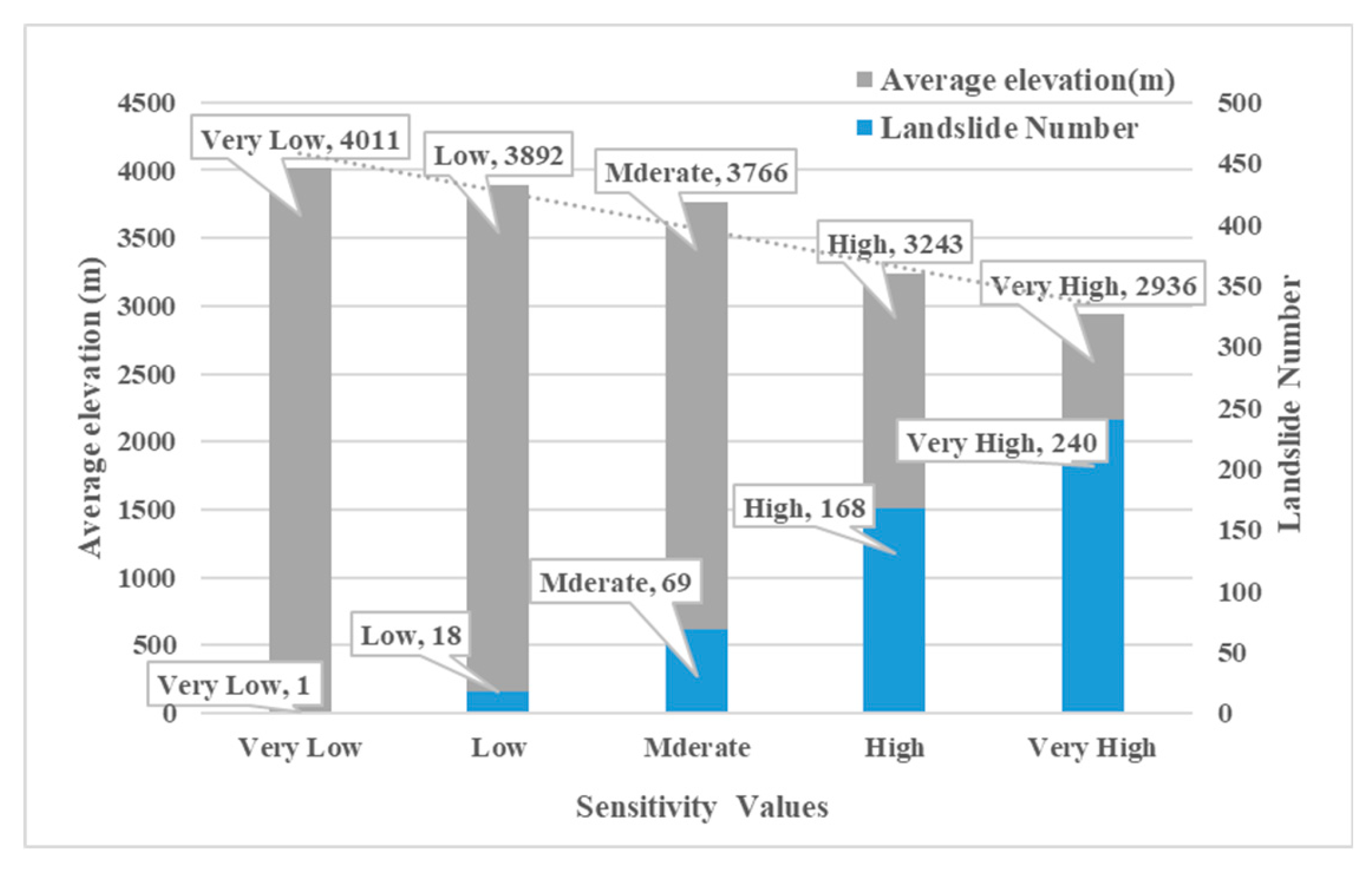
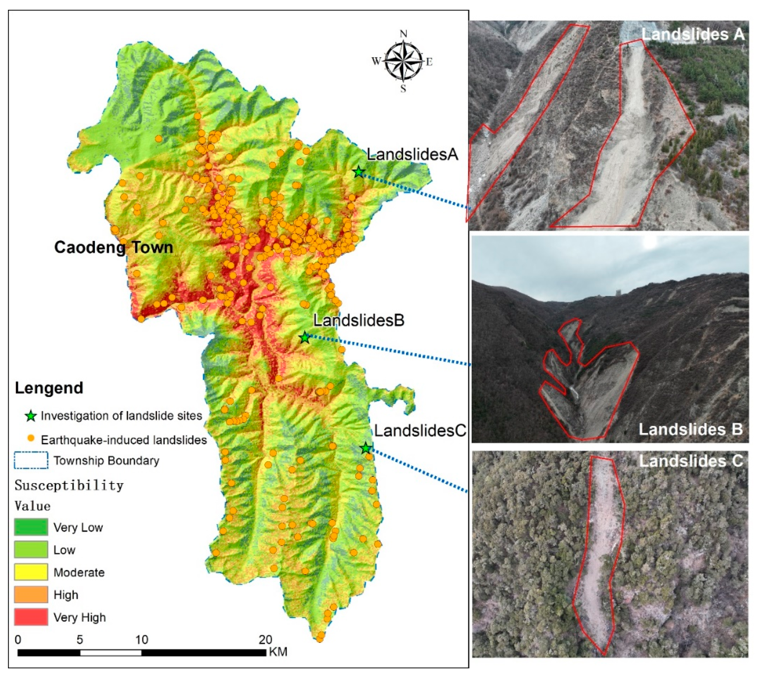
Selecting the best-performing coupled model from preliminary studies, Caodeng Township was chosen as the investigation area. The analysis revealed that high susceptibility zones accounted for 45% of the county’s total area. Data analysis indicated that there were 496 landslides in this region, among which 408 (82.25%) were located in high and very high susceptibility zones, while 88 (17.75%) were situated in areas with moderate-to-low susceptibility (
Figure 10). Although the accuracy is within an acceptable range, it is necessary to explore the actual causes of these errors to further improve model precision.
Data analysis and field investigations have helped identify some potential reasons for these discrepancies. As shown in the figure, an inverse relationship between elevation and landslide occurrence was observed, suggesting that the model’s errors are primarily concentrated in higher-altitude areas. Through an in-depth analysis of the evaluation methodology and field surveys, we further identified two potential reasons for this phenomenon.
The first issue is the concealment of high-altitude landslides. As shown in
Figure 11, landslides A, B, and C are located in high-altitude areas with low or very low susceptibility. These regions are characterized by minimal human activity, distance from river systems, and high levels of vegetation or snow cover, which often result in lower susceptibility assessment outcomes. However, due to the tensile stress exerted along mountain ridges, these landslides tend to develop concealed crack propagation, and seismic activity accelerates their occurrence. Secondly, the accuracy of machine learning models is highly dependent on the sample data. The adaptability of different methods varies across different environmental conditions, making a more comprehensive and accurate dataset indispensable. Additionally, analyzing the applicability of different models to various conditions should be a key focus in future research.
5. Conclusions
This study focuses on the comparative analysis of landslide susceptibility assessment models. The findings indicate that the traditional information value model has notable limitations in accuracy. Since it is based on fixed weights and simple statistical relationships, it struggles to fully capture the dynamic interactions among influencing factors in complex geological environments, thereby restricting its precision in landslide susceptibility evaluation.
Compared to traditional statistical methods, machine learning approaches demonstrate significant improvements in accuracy. With their strong nonlinear fitting capabilities, these models can uncover hidden complex patterns within data. However, machine learning methods are not flawless—they are prone to overfitting, exhibit weak generalization ability for small sample datasets, and have poor interpretability, making it difficult to directly understand the specific impact mechanisms of different factors on landslide susceptibility.
In contrast, hybrid models integrate the advantages of both traditional statistical and machine learning methods, achieving a complementary effect. On the one hand, they enhance interpretability by leveraging the theoretical foundation of statistical methods. On the other hand, they utilize the efficient data processing and pattern recognition capabilities of machine learning to improve adaptability to complex data. The hybrid models outperform both individual approaches in accuracy, providing a more precise evaluation of landslide susceptibility and offering a more reliable scientific basis for landslide disaster prevention and mitigation.
Author Contributions
Bu Xianghang: Conceptualization, Methodology, Writing – original draft. Fan Songhai: Funding acquisition, Writing – review & editing. Zhang Zongxi: Investigation. Zhu Ke: Investigation. Ma Xiaomin Investigation. Li Ning: Writing – review & editing.
Funding
This research was supported by the State Grid Sichuan Electric Power Company Technology Project (52199723001D).
References
- Liang, Y.L.; et al. Analysis of Seismic Intensity Distribution and Building Damage Characteristics of the M_S 6.0 Earthquake Swarm in Barkam. Seismological and Geomagnetic Observation and Research 2023, 44, 28–35. [Google Scholar]
- Fan, X.M.; et al. Study on the Characteristics and Spatial Distribution Rules of Geological Disasters Induced by the M_S 6.8 Luding Earthquake in 2022. Journal of Engineering Geology 2022, 30, 1504–1516. [Google Scholar]
- Huang, F.; et al. Comparisons of heuristic, general statistical and machine learning models for landslide susceptibility prediction and mapping. Catena 2020, 191, 104580. [Google Scholar] [CrossRef]
- Yan, J.S.; Tan, J.M. Landslide Susceptibility Evaluation Based on Different Factor Classification Methods: A Case Study of Yuan’an County, Hubei Province. The Chinese Journal of Geological Hazard and Control 2019, 52–60. [Google Scholar]
- Huang, F.M.; Cao, Z.S.; Yao, C.; et al. Landslide Hazard Early Warning Based on Decision Tree and Effective Rainfall Intensity. Journal of Zhejiang University (Engineering Science) 2021, 55, 472–482. [Google Scholar]
- He, Q.; et al. Landslide and Wildfire Susceptibility Assessment in Southeast Asia Using Ensemble Machine Learning Methods. Remote Sensing 2021, 13, 1572. [Google Scholar] [CrossRef]
- Wang, Z.; Liu, Q.; Liu, Y. Mapping Landslide Susceptibility Using Machine Learning Algorithms and GIS: A Case Study in Shexian County, Anhui Province, China. Symmetry 2020. [Google Scholar] [CrossRef]
- Jia, Y.F.; Wei, W.H.; Chen, W.; et al. Landslide Susceptibility Evaluation Based on the SOM-I-SVM Coupling Model. Hydrogeology & Engineering Geology 2023, 50, 125–137. [Google Scholar]
- Li, G.Y.; Liu, P.; Zhang, K.; et al. Influence Analysis of Dimensionality Unification in Landslide Susceptibility Evaluation. Hydrogeology & Engineering Geology 2024, 51, 118–129. [Google Scholar]
- Peng, S.Q.; et al. Regional Landslide Hazard Evaluation and Zoning Using the Coupling Model of Information Value Method and Random Forest and the Critical Monthly Average Rainfall Threshold: A Case Study of Fuling District, Chongqing City. The Chinese Journal of Geological Hazard and Control 2025, 36, 131–145. [Google Scholar]
- Zhang, J.Y.; et al. Preliminary Analysis of Emergency Products and Focal Parameters of the M6.0 Earthquake in Barkam, Sichuan on June 10, 2022. Earthquake Research in China 2022, 38, 370–382. [Google Scholar]
- .Xu, X.W.; et al. Discovery of the Longriba Fault Zone in the Eastern Bayan Har Block and Its Tectonic Significance. Science in China Series D Earth Sciences 2008, 529–542. [Google Scholar]
- Xiao, B.F.; et al. Quantitative Assessment of Earthquake Damages with Visualization of Typical Scenarios Based on Oblique Photogrammetry Technology: A Case Study of the Earthquake Swarm in Barkam, Sichuan. Seismology and Geology 2023, 45, 847–863. [Google Scholar]
- Sun, D.; et al. Activity and Effect of Main Faults in Near Field of Bala Hydropower Station in Barkam. Journal of Engineering Geology 2010, 18, 940–949. [Google Scholar]
- Xu, C.; et al. Study on the Occurrence Probability of Coseismic Landslides: A New Generation of Seismic Landslide Hazard Model. Journal of Engineering Geology 2019, 27, 1122–1130. [Google Scholar]
- Wang, T.H.; et al. Monthly Prevention and Control Perspective on Geological Hazard Risk Assessment in Towns Along the Lower Hanjiang River. People’s Yangtze River 2024, 55, 98–107. [Google Scholar]
- Wu, X.G.; et al. Landslide Susceptibility Evaluation in Towns of the Hengduan Mountainous Area in Yunnan Province. Journal of Geological Hazards and Environmental Protection 2023, 34, 13–19. [Google Scholar]
- Chen, Z.H. Hazard Risk Assessment of Mountain Disasters Based on the AHP-Information Value Model. Science and Technology & Innovation 2024, 6, 118–120. [Google Scholar]
- Wu, M.T.; Sun, Y.; Zhou, Z.T. Landslide Susceptibility Evaluation Based on the Analytic Hierarchy Process-Information Quantity Method: A Case Study of Fuliang County, Jiangxi Province. Journal of East China University of Technology Natural Science Edition 2023, 46, 157–166. [Google Scholar]
- Chen, T.; Guestrin, C. XGBoost: A Scalable Tree Boosting System. ACM, 2016.
- Catani, F.; et al. Landslide susceptibility estimation by random forests technique: Sensitivity and scaling issues. Natural Hazards and Earth System Sciences 2013, 13, 2815–2831. [Google Scholar] [CrossRef]
- Breiman, Random forests. Mach Learn 2001, 45, 5–32.
- Pradhan, B. Manifestation of an advanced fuzzy logic model coupled with Geo-information techniques to landslide susceptibility mapping and their comparison with logistic regression modelling. Environmental and Ecological Statistics 2011, 18, 471–493. [Google Scholar] [CrossRef]
- Information, V.F.A.; et al. Landslide spatial prediction based on cascade forest and stacking ensemble learning algorithm.
- Fawcett, T. An introduction to ROC analysis. Pattern Recognition Letters 2005, 27, 861–874. [Google Scholar] [CrossRef]
- Pourghasemi, H.R.; Pradhan, B.; Gokceoglu, C. Application of fuzzy logic and analytical hierarchy process (AHP) to landslide susceptibility mapping at Haraz watershed, Iran. Natural Hazards 2012, 63, 965–996. [Google Scholar] [CrossRef]
- Liu, Y.T. Landslide Susceptibility Evaluation Based on Multi-Source Data Factor Extraction and Optimization. China University of Geosciences (Beijing), 2023.
- Information, V.F.A.; et al. Landslide spatial prediction based on cascade forest and stacking ensemble learning algorithm.
|
Disclaimer/Publisher’s Note: The statements, opinions and data contained in all publications are solely those of the individual author(s) and contributor(s) and not of MDPI and/or the editor(s). MDPI and/or the editor(s) disclaim responsibility for any injury to people or property resulting from any ideas, methods, instructions or products referred to in the content. |
© 2025 by the authors. Licensee MDPI, Basel, Switzerland. This article is an open access article distributed under the terms and conditions of the Creative Commons Attribution (CC BY) license (http://creativecommons.org/licenses/by/4.0/).