
Submitted:
21 May 2025
Posted:
23 May 2025
You are already at the latest version
Abstract
Machine learning techniques have been increasingly used in flood management worldwide to enhance the effectiveness of traditional methods for flood susceptibility mapping. Although these models have achieved higher accuracy than traditional ones, their application has not yet reached full maturity. We focus on applying machine learning models to create flood susceptibility maps (FSMs) for Thessaly, Greece, a flood-prone region with extreme flood events recorded in recent years. The study utilizes 13 explanatory variables derived from topographical, hydrological, hydraulic, environmental and infrastructure data to train the models, using the Daniel storm—one of the most severe recent events in the region—as the primary reference for model training. The most significant of these variables were obtained from satellite data of the affected areas. Four machine learning algorithms were employed in the analysis, i.e., Logistic Regression (LR), Support Vector Machine (SVM), Random Forest (RF), and eXtreme Gradient Boosting (XGBoost). Accuracy evaluation revealed that tree-based models (RF, XGBoost) performed better, achieving Area Under the Curve (AUC) values of 97%. A flood susceptibility map corresponding to a 1000-year return period rainfall scenario at 24 h scale was developed, aiming to support long-term flood risk assessment and planning. The results demonstrate the potential of machine learning in providing accurate and practical flood risk information to enhance flood management and support decision-making for disaster preparedness in the region.
Keywords:
flood susceptibility mapping (FSM)
; machine~learning (ML)
; LR
; SVM
; RF
; XGBoost
; Greece
; Thessaly
; Daniel
1. Introduction
1.1. General and Literature Review
Flood events are natural phenomena in which normally dry land becomes inundated due to excessive water accumulation. These result in devastating consequences worldwide, causing significant economic, environmental, and social impacts [1,2]. They originate from various factors, including intense or prolonged rainfall, river overflow, storm surges, and dam failures. Floods are a global challenge, affecting regions regardless of geographical boundaries and endangering millions of lives. Their impact highlights the need for continuous research and strategic planning to mitigate associated risks. To this end, in the framework of the implementation of the European Union Flood Directive [3] the assessment and management of flood risk have been prioritized. Floods can be categorised according to their origin, root cause, and occurrence, as river floods, flash floods, coastal floods, urban floods and floods induced by the failure of respective flood protection structures [4,5]. Effective flood management is crucial for minimizing damage to communities, infrastructure, and the environment.
As suggested by the current legal framework (i.e., Floods Directive 2007/60/EC [3]), flood susceptibility and hazard maps are essential at the river basin level. By the term Flood Susceptibility Map (FSM) we refer to a spatial representation of a region or river basin that identifies areas that are prone to flooding. These maps help to highlight regions with a higher likelihood of flooding, considering various factors, e.g., topography, rainfall, land use and historical floods. On the other hand, Flood Hazard Maps (FHM) measure the water depth and extent across a flooded area. They play a crucial role in risk assessment, land-use planning, and the development of effective flood management strategies.
Traditionally, flood susceptibility mapping has been conducted using a variety of qualitative and quantitative approaches. Qualitative methods, such as Multi-Criteria Decision Analysis (MCDA) [6], integrate expert knowledge and spatial criteria to evaluate flood-prone areas. Statistical approaches, including linear regression and frequency ratio analysis [7], are utilized to assess the relationships between historical flood occurrences and influencing factors. Hydrological-based models, including HyMOD [8] and the Soil and Water Assessment Tool (SWAT) [9], simulate the hydrological cycle to estimate surface runoff and flood potential. Additionally, hydraulic models, such as the Hydrologic Engineering Center’s River Analysis System (HEC-RAS) [10], are employed to simulate water flow dynamics and floodplain extents based on channel geometry and discharge data. These conventional methods, while widely used, often require large amounts of data, which must be weighted by selecting appropriate weights, and often require time-consuming flood simulations that are based on numerical models, which, in turn, also depend on the discretization of the physical domain.
To address above limitations, alternative approaches such as Machine Learning (ML) and Deep Learning (DL) models have been explored in flood susceptibility mapping, offering potential benefits in terms of efficiency and accuracy. ML models can handle large and complex datasets, identify non-linear relationships and complicated patterns. Extensive research has been conducted on the application of these models across various river basins worldwide. A comprehensive literature review of 58 recent publications has been presented in [4], covering various aspects of flood mapping, including flood inundation, flood susceptibility, and flood hazard, with a focus on DL approaches. Various ML algorithms have been employed for flood susceptibility mapping. In particular, Artificial Neural Networks (ANN), Multi-Layer Perceptron (MLP), Least absolute shrinkage and selection operator (Lasso) have been used in [11], as well as Random Forest (RF), Support Vector Machine (SVM), Convolutional Neural Network (CNN) in [12]. Additionally, various boosting algorithms, such as AdaBoost, Gradient Boosting, XGBoost, CatBoost, and Stochastic Gradient Boosting (SGB), have been utilized [13]. Table 1 presents a brief summary of selected studies in this field. For each algorithm listed in the table, the best-performing model is highlighted in bold. In Table 2 lists the flood conditioning factors used in the respective studies, which serve as inputs for the corresponding models. Although machine learning models are pretty powerful tools, they require a significant amount of high-quality and labeled data for training. If the data is limited, biased, or unreliable, their accuracy can suffer—making them less effective, especially in areas with little historical flood data. However, unlike traditional methods, they can often work with smaller, more focused datasets or utilize techniques like data augmentation and transfer learning to improve accuracy.
Machine learning models can be very useful when combined with satellite data, offering state-of-the-art, data-driven methods for analyzing large-scale patterns. Satellite imagery offers high-resolution, real-time data on some of the most important flood-influencing variables such as topography, land cover, soil moisture, precipitation, as well as the flooded area. ML algorithms can process and analyze these large datasets to detect patters, flood-prone areas, identify the most influencing features, and improve predictive accuracy. Flood conditioning factors serve as input to the model (independent variables), while the output (depended variable) determines whether an area is classified as flooded or not. This process can be framed as either a classification or regression problem, depending on the nature of the output values. By integrating ML with satellite observations, researchers can enhance flood prediction capabilities, even in regions with limited ground-based hydrological data [14]. However, challenges such as data preprocessing, cloud cover interference, and model interpretability remain key considerations in optimizing the use of ML for satellite-based flood susceptibility mapping.
Despite the widespread use and numerous applications of ML models for FSM globally, their adoption in Greek basins remains limited. This is largely due to challenges such as a lack of technical expertise and the relatively early stage of ML integration into flood management practices. An attempt was made in [15] at the national scale for flood hazard mapping using multi-criteria analysis and ANN. The full potential of ML in FSM remains underexplored. Similar barriers to ML adoption exist in other regions as well, where limited resources and expertise block broader implementation. Smaller regions and basins should also be considered for flood susceptibility mapping to improve accuracy and obtain more region-specific results. Thessaly, the focus of this study, is a flood-prone region that has faced severe flood events in recent years, highlighting the importance of flood susceptibility mapping. One of the most recent extreme events was Storm "Daniel" in September 2023, which resulted in devastating damages [16]. The Storm Daniel, also known as Cyclone Daniel, took place on 4-7 September 2023. It affected not only Greece but also Bulgaria, Turkey, and Libya, causing extensive flooding. A post-event analysis of Storm Daniel in Thessaly [17] revealed that the Peneus river basin received an average rainfall of approximately 360 mm, which triggered extensive flooding. The disaster resulted in the loss of human lives and caused severe environmental and economic damage. The study calculated that although the station based return period point estimates exhibited substantial variability, the overall area averaged return period for the 72 h time-scale reached up to 150 years, reflecting the remarkable intensity of the event.

Table 1.
Summary of selected machine learning applications for FSM. The best-performing model from each study is highlighted in bold.
Table 1.
Summary of selected machine learning applications for FSM. The best-performing model from each study is highlighted in bold.
| Area of Interest | Algorithms | Evaluation | Data Split train/test (%) |
Total Points | Resolution (m) |
Ref |
|---|---|---|---|---|---|---|
| Ibaraki, Japan |
ANN-MLP SVR GBR Lasso |
MAE MSE RMSE R2 AUC / ROC |
70/30 | 224 | 30×30 | [11] |
| Berlin, Germany | CNN ANN RF SVM |
AUC / Kappa | 80/20 | 3934 | 30×30 10×10 5×5 2×2 |
[12] |
| Idukki, Kerala India | AdaBoost Gradient Boosting XGBoost CatBoost SGB |
AUC Precision Recall NP |
70/30 | 1500 | 30×30 | [13] |
| Periyar River, India | LR SVM Naive Bayes RF Ada Boosting Gradient Boosting XGBoost |
AUC / ROC | 30/70 | 188 | 30×30 | [18] |
| Fujairah, UAE |
xDeepFM DNN SVM RF |
recall precision accuracy |
75/25 | 2400 | 30×30 | [19] |
| Salzburg, Austria | MCDA (AHP, ANP) ML (RF, SVM) |
AUC / ROC | 70/30 | 30×30 | [20] | |
| Metlili, Morocco |
RF CART SVM XGBoost |
AUC | 70/30 | 204 | 30×30 | [21] |
| Karun, Iran Gorganrud, Iran |
Deep Forest CFM Multi-gained scanning |
AUC / ROC OA KC |
27/73 | 4160 1278 |
30×30 | [22] |
| Wilayat As-Suwayq, Oman |
XGBoost RF CatBoost |
AUC | 70/30 | 446 | 5×5 | [23] |
| Haraz, Iran | ANN CART FDA GLM GAM BRT MARS MaxEnt |
AUC / ROC | – | 201 | 20×20 | [24] |
* ANN: Artificial Neural Network, MLP: Multilayer Perceptron, SVR: Support Vector Regression, GBR: Gradient Boosting Regressor, CNN: Convolutional Neural Network, RF: Random Forest, XGBoost: eXtreme Gradient Boosting, SVM: Support Vector Machine, SGB: Stochastic Gradient Boosting, LR: Logistic Regression, xDeepFM: eXtreme Deep Factorisation Machine, DNN: Deep Neural Network, AHP: Analytical Hierarchical Process, ANP: Analytical Network Process, CART: Classification And Regression Trees, CFM: Cascade Forest Model, FDA: Flexible Discriminant Analysis, GLM: Generalized Linear Model, GAM: Generalized Additive Model, BRT: Boosted Regression Trees, MARS: Multivariate Adaptive Regression Splines, MaxEnt: Maximum entropy.
Table 2.
Flood conditioning factors used in each of the selected machine learning applications for FSM.
Table 2.
Flood conditioning factors used in each of the selected machine learning applications for FSM.
| Ref | Flood Conditioning Factors |
|---|---|
| [11] | Elevation, Slope, Aspect, Plane curvature, Profile curvature, TWI, SPI, DTStreams, DTRiver, DTRoads, Land Cover |
| [12] | Elevation, Slope, Aspect, Curvature, TWI, DTRiver, DTRoads, DTDrainage, CN, AP, FP |
| [13] | Elevation, Slope, Aspect, Curvature, STI, TRI, TWI, SPI, DTRoads, DTStreams, Soil, Geology,Geomorphology, LULC, NDVI, Rainfall |
| [18] | Elevation, Slope, Aspect, Flow direction, Drainage Density, SPI, STI, TPI, NDWI, Rainfall |
| [19] | Elevation, Slope, Curvature, Drainage Density, SPI, TWI, STI, TRI, NDVI, DTDrainage, Rainfall, Land Use, Geology |
| [20] | Elevation, Slope, Aspect, TWI, SPI, DTRoads, DTDrainage, NDVI, Geology, Rainfall, Land Cover |
| [21] | Elevation, Slope, Aspect, Plan curvature, TWI, SPI, DTStreams, DTRoads, Lithology, Rainfall, LULC, NDVI |
| [22] | Elevation, Slope, Aspect, Curvature, Plan Curvature, Profile Curvature, TPI, TRI, TWI, SPI, Convergence Index, LULC, NDVI, Valley Depth, LS Factor, Flow Accumulation, MCA, HOFD, VOFD, CN, MFI |
| [23] | Elevation, Slope, Curvature, TRI, TWI, SPI, DTDrainage, Drainage density, DTRoads, NDVI, Geology, Soil Type, Rainfall |
| [24] | Elevation, Slope, Curvature, SPI, TWI, River Density, DTRiver, NDVI, Land cover, Lithology, Rainfall |
* TWI: Topographic Wetness Index, SPI: Stream Power Index, STI: Sediment Transport Index, TPI: Topographic Position Index, TRI: Topographic , DTStreams: Distance from Streams, DTRiver: Distance from Rivers, DTRoads: Distance from Roads, DTDrainage: Distance from Drainage, CN: Curve Number, AP: Annual Precipitation, FP: Frequency Precipitation, NDVI: Normalized Difference Vegetation Index, LULC: Land Use Land Cover, NDWI: Normalized Difference Water Index, MCA: Modified Catchment Area, HOFD: Horizontal Overland Flow Distance, VOFD: Vertical Overland Flow Distance, MFI: Modified Fournier Index.
1.2. Objectives and Structure of the Study
This paper focuses on making flood susceptibility mapping on Peneus River Basin (PRB) with machine learning algorithms, contributing to the advancement of data-driven approaches in flood risk assessment. The first objective is to evaluate and compare the performance of various machine learning models—Logistic Regression (LR), Support Vector Machine (SVM), Random Forest (RF), eXtreme Gradient Boosting (XGBoost)—during an extreme flood event, specifically the Storm Daniel. Thereafter, to further investigate the predictive capability and generalizability of the most effective model, the best model was applied under different initial training conditions. Finally, a flood susceptibility map corresponding to a 1000-year return period rainfall scenario was generated.
The contributions of the present paper can be outlined as follows:
- Support the development of an early warning system for flood susceptibility through the exploitation of satellite-derived rainfall data.
- Application and comparative analysis of machine learning models (LR, SVM, RF, XGBoost) to produce accurate flood susceptibility maps.
- Calculation of feature importance scores to evaluate the influence of each input variable on model predictions.
- Investigation of the impact of different initial training conditions on model performance.
- Development of a FSM based on a 1000-year return period rainfall scenario at 24 h scale.
- Provision of recommendations for flood risk management and planning in the case study, based on the results obtained.
The novelty of the paper lies in the application of state-of-the-art machine learning methods for flood susceptibility mapping, taking into account an extreme event that affected the a challenging region. Thessaly is an ideal case study due to its challenging topography, which includes extensive lowland areas that make it suitable for model testing. Even though the applied machine learning models are well-established and have been widely adopted in previous research work, we investigate them in Peneus watershed. This approach offers a localized perspective that enables customized flood risk management strategies and adaptation measures. By applying these advanced ML techniques to the Peneus watershed, this study contributes to the growing maturity of ML in FSM, addressing gaps in previous research and providing insights that have yet to be explored in similar contexts. The integration of regional data with a real-world extreme event enhances the practical relevance and transferability of the proposed methodology, offering valuable insights to authorities for informed decision-making.
Following the Introduction (Section 1), which underscores the importance of generating FSMs and reviews the methodologies employed, particularly machine learning techniques, the paper is structured as follows: The methodological framework is detailed in Section 2, while the used data and the case study are described in Section 3. The results, including the simulation and experimentation outcomes and comparisons between different models are presented in Section 4, followed by a broader discussion in Section 5. Finally, Section 6 summarizes the key findings and conclusions of this study.
2. Material and Methods
There are several ways to develop a model for flood susceptibility analysis. One approach treats it as a regression problem, predicting water depth as a continuous variable. Another frames it as a classification task, distinguishing between flooded and non-flooded areas. In this study, we adopt a classification approach, where the objective is to predict the likelihood of a location being classified as either flooded (1) or non-flooded (0), based on a set of input variables. Those explanatory variables are some factors, also referred to as flood conditioning factors, which significantly influence the probability of flooding. The selected factors are briefly described in Section 3.3. In general we create a dataset comprising some independent variables (flood conditioning factors) and a single dependent variable (classified as flood-prone or not flood-prone). This setup formulates a binary classification task suitable for machine learning applications. The overview of the methodology is depicted in Figure 1. Four well established machine learning models have chosen to support this approach (i.e., Logistic Regression, Support Vector Machine, Random Forest and Extreme Gradient Boosting). Their underlying mechanisms and limitations are discussed in the following sections.
2.1. Logistic Regression (LR)
Logistic Regression (LR) [25] is a supervised machine learning algorithm commonly used to predict the probability of categorical outcome, particularly in binary classification tasks, where the goal is to distinguish between two classes. The key characteristic of logistic regression is that it models the relationship between the input features and the output probability using an S-shaped curve (Figure 2), known as the logistic or sigmoid function (Equation 1). This ensures that the predicted values are always restricted between zero and one, allowing them to be interpreted as probabilities.
where z is a linear combination of the input features and their corresponding weights; x is the feature vector, w is the weight vector and is the bias term. The wights are determined during training process with maximum-likelihood estimation algorithm [26]. LR is simple, interpretable, and efficient for binary classification tasks, especially when the relationship between input and output is approximately linear. However is struggles with more complex relationships and non-linear decision boundaries.
2.2. Support Vector Machine (SVM)
Support Vector Machine (SVM) [27] is a supervised machine learning algorithm commonly used for binary classification, though it can also be applied to regression tasks. SVM’s goal is to find the optimal decision boundary or hyperplane (for > 3 features) that separates the data into two or more classes, while maximizing the margin between them. An example of the model key characteristics is depicted in Figure 3.
Mathematically, the decision boundary (hyperplane) in linear SVM can be described by the equation 3:
where x is the input vector, w is the weight vector and is the bias term. Parameters are calculated through solving an optimization problem that aims to find the hyperplane which maximizes the margin. When data points are not linearly separable in their original space, SVM uses the kernel trick [28] to map them into a higher-dimensional space where a linear separation is possible. Common kernels include the linear, polynomial, radial basis function (RBF), and sigmoid kernels, which measure similarity between data points to enable effective separation. SVM is effective in high-dimensional spaces and remains memory-efficient by relying only on a subset of training points (support vectors) to determine the decision boundary, but careful normalization is required. At the same time it is computationally intensive and slow to train on large datasets, which can negatively impact scalability and performance.
2.3. Random Forest (RF)
Random Forest (RF) [29] is an ensemble learning algorithm widely used for classification and regression tasks. It operates by constructing a large number of decision trees [30] during training and outputting the class that is the majority vote of the individual trees. Each tree is trained on a random subset of the data (using a bootstrapping sampling), and at each split, it considers a random subset of features, which helps reduce overfitting and improves generalization. This randomness ensures that the trees are independent, making the overall model more robust than a single decision tree. The final prediction for a classification problem is typically the class with the most votes among all trees. Figure 4 summarizes the architecture of RF model. Random Forests are particularly effective in handling high-dimensional data, capturing non-linear relationships, and working well with both numerical and categorical features, in tabular form. However, they can be computationally expensive for large datasets and are less interpretable than simpler models like logistic regression. Despite this, their accuracy, resistance to overfitting, and minimal need for parameter tuning make them a powerful tool in prediction assessment.
2.4. Extreme Gradient Boosting (XGBoost)
XGBoost (eXtreme Gradient Boosting) [31] is a high-performance machine learning algorithm built upon the gradient boosting framework and has gained widespread recognition due to its success in numerous Kaggle competitions [32]. It operates as an ensemble method, meaning it combines multiple base learners—typically decision trees [30]—through a boosting process. In this process, models are trained sequentially, with each one aiming to reduce the errors made by its predecessors. This iterative optimization leads to continuous performance improvement by minimizing a defined objective function. Boosting techniques like XGBoost are particularly effective at balancing bias and variance. In the case of XGBoost, each decision tree assigns a numerical weight to its leaf nodes, and samples are directed to these leaves based on their feature values, with the leaf’s weight representing the prediction. The term "gradient" in gradient boosting refers to the use of gradient descent to minimize errors as more models are added. XGBoost distinguishes itself from other boosting algorithms through the inclusion of regularization within its objective function to prevent overfitting and its capability to build trees in parallel, greatly enhancing computational speed. These features contribute to its reputation as a highly efficient, flexible, and scalable algorithm. The architecture and training process of XGBoost are illustrated in Figure 5.
Following [31], the objective function that needs to be minimized at t-th iteration is:
where is the target value, is the prediction, l is a differentiable loss function, is the output of the new model at iteration t, and n is the number of training samples. The first term of Equation (4) measures how well the model perform on training data, and the second term is a regularization term that measures the complexity of the base learners (i.e., trees), to avoid overfitting. In Equation (5) T stands for the number of leaves in the tree, with leaf weights w, and , are regularization parameters. The task of optimizing this objective function can be simplified to minimizing a quadratic function, by using the second order Taylor expansion [33].
The key difference between RF and XGBoost is that RF, being a bagging model, generates decision trees and calculates their predictions in parallel. One the other hand, XGBoost algorithm is a sequential model, which means that each subsequent tree is dependent on the outcome of the last one. XGBoost is sensitive to hyperparameters and careful tuning is required to achieve good performance. This process can lead to pretty high optimization, particularly when working with large datasets. The model only accepts numerical values for processing. Additionally, the model’s complexity makes it less interpretable compared to simpler algorithms.
2.5. Feature Importance
With the expanding use of machine learning in decision-making, it is becoming ever more important to ensure transparency and to understand the factors contributing to a model’s predictions [34]. Feature Importance (FI) in ML refers to techniques used to quantify the contribution each input feature to the model’s prediction. Understanding which features are most influential helps improve model transparency, supports better feature selection, and can reveal insights about the underlying data. There are several ways to calculate feature importance, such as [35]:
- Coefficient-based feature importance
- Permutation-based feature importance
- Tree-based feature importance
- SHapley Additive exPlanations (SHAP)
Coefficient-based FI is used in linear models (like linear or logistic regression), where the magnitude of the model coefficients indicates the relative importance of each feature. Permutation-based FI measures the impact of each feature on model performance by randomly shuffling its values and observing the decrease in metrics. In tree-based model like (RF, XGBoost etc.) FI is typically calculated based on how much each feature reduces impurity (e.g., Gini impurity or entropy) [36]. SHAP [37] is a model-agnostic method based on cooperative game theory. It gives a clear way to see how much each feature contributes to a model’s prediction by looking at how the prediction changes, when you include or exclude that feature in different combinations. This makes SHAP a valuable tool for understanding model behavior. SHAP feature importance serves as an alternative to permutation-based feature importance. While permutation importance evaluates the impact of a feature by measuring the decrease in model performance when the feature values are randomly shuffled, SHAP quantifies importance based on the magnitude of feature attributions derived from their contributions to individual predictions. By identifying key drivers of a model’s output, feature importance aids in building more interpretable and efficient models.
2.6. Evaluation Metrics
Selecting the appropriate evaluation metrics is essential during the model assessment phase, as they offer a clear understanding of the model’s effectiveness in practical applications. In binary classification tasks, which is our case, the choice of metrics significantly impacts how performance is interpreted [38]. The most popular and used metric to evaluate the performance of classification models is accuracy. Accuracy is simply measures the overall proportion of correct predictions with respect to the total number of data. While accuracy gives an overall idea of a model’s performance, it can be a misleading metric in some cases like imbalanced datasets. To overcome the drawbacks we usually use more metrics like precision, recall, specificity, , which provide a more detailed evaluation, especially when dealing with imbalanced data or situations where different types of errors have different costs. Precision indicating the proportion of true positives among predicted positives, and recall 9or sensitivity) indicating the proportion of true positives among actual positives. Specificity provides the number of negative records correctly predicted. combines precision and recall into one metric, by calculating the harmonic mean.
Additionally, Receiver Operating Characteristic (ROC) curves and the corresponding Area Under the Curve (AUC) are widely used for binary classification algorithms to evaluate a model’s ability to rank positive instances higher than negatives across various threshold settings. The ROC curve is produced by calculating and plotting the True Positive Rate (TPR) in y-axis, against the False Positive Rate (FPR) in x-axis, for a classifier at a variety of thresholds. A good model will have a large ROC-AUC, while a poor model will be positioned near the diagonal line, which represents random performance. The ROC-AUC metric is also very useful for comparing different models against each other. Selecting appropriate metrics depends on the specific goals of the task, particularly in cases of class imbalance where accuracy alone can be misleading.
Equations (6)–(10) present the formulas for the aforementioned metrics.
where stands for True Positive, True Negative, False Positive, and False Negative respectively. To elaborate, each term means:
- True Positive: the number of instances where the model correctly predicted the positive class,
- True Negative: the number of instances where the model correctly predicted the negative class,
- False Positive: the number of instances where the model incorrectly predicted the negative class for a positive case and,
- False Negative: the number of instances where the model incorrectly predicted the positive class for a negative case.
3. Data
3.1. Study Area
The selected study region is the Peneus river basin (Figure 6), situated in Thessaly, Greece. Peneus basin occupies approximately 85% of the Thessaly Water District, covering a total area of 11,062 km2. Thessaly’s topography is defined by four surrounding mountain ranges: Olympus-Kamvounia to the north, Pindus to the west, Othrys to the south, and Pelion-Ossa to the east. Originating in the Pindus Mountains, the Peneus river traverses the Thessalian Plain and discharges into the Aegean Sea. The region exhibits a transition from a Mediterranean climate to an eastern coastal climate. Climatic conditions vary geographically, with a continental climate prevailing in the central lowlands and a mountainous climate in the western highlands. Annual precipitation is highest in the western highlands and decreases toward the lowlands, before increasing again in the eastern highlands, and it is strongly seasonal [39]. The average annual temperature ranges between 16–17 °C. The region holds significant importance due to its extensive agricultural activity, encompassing approximately 450,000 hectares (ha) of agricultural land, of which 250,000 hectares (ha) are irrigated. We have selected to apply the aforementioned methodology in the Peneus river basin due to its regional significance and the recurring flood-related challenges it faces, including extreme events [40]. The area has experienced numerous flood events over time [41]. Two of the most recent and significant flood events were caused by Mediterranean cyclone Ianos (18-20 September 2020) [42] and Daniel Storm (4-7 September 2023) [17]. Both events resulted in loss of life and extensive damage to infrastructure and agricultural land. Among them, Storm Daniel was the most intense, causing widespread inundation and catastrophic impacts, which is why we selected as the main event of this study. After each similar event, the case for preventive measures is revived, yet no substantial intervention follows from the responsible authorities.
3.2. Flood Inventory Map
Flood maps are fundamental for identifying and extracting samples of flooded and non-flooded areas. The accuracy of this inventory dataset directly influences the potential reliability of the models. In this context, we created a flood inventory map using the most recent significant flood event, i.e. the Daniel flood event in September 2023. Synthetic Aperture Radar (SAR) image data used to identify the flooded area of the catchment by this event, and more specifically Sentinel-1 mission (https://browser.dataspace.copernicus.eu/ (accessed 10 February 2025)). The flood extent was derived by processing satellite images captured before and after the flood event—on 30 August 2023 and 07 September 2023, respectively (https://rapidmapping.emergency.copernicus.eu/EMSR692/download (accessed 10 February 2025)). The flood coverage is highlighted in Figure 7. The flooded and non-flooded ares were assigned a value of "1" (positive class) and a values of "0" (negative class). From the derived inventory map of the watershed, 3 950 data points were randomly selected to create our dataset for the modeling. The selection process ensured the dataset remained balanced, maintaining an equal ratio of flooded and non-flooded points. This initial dataset was divided into 80 % for training and validation purposes and the rest 20 % for testing the models.
3.3. Flood Conditioning Factors
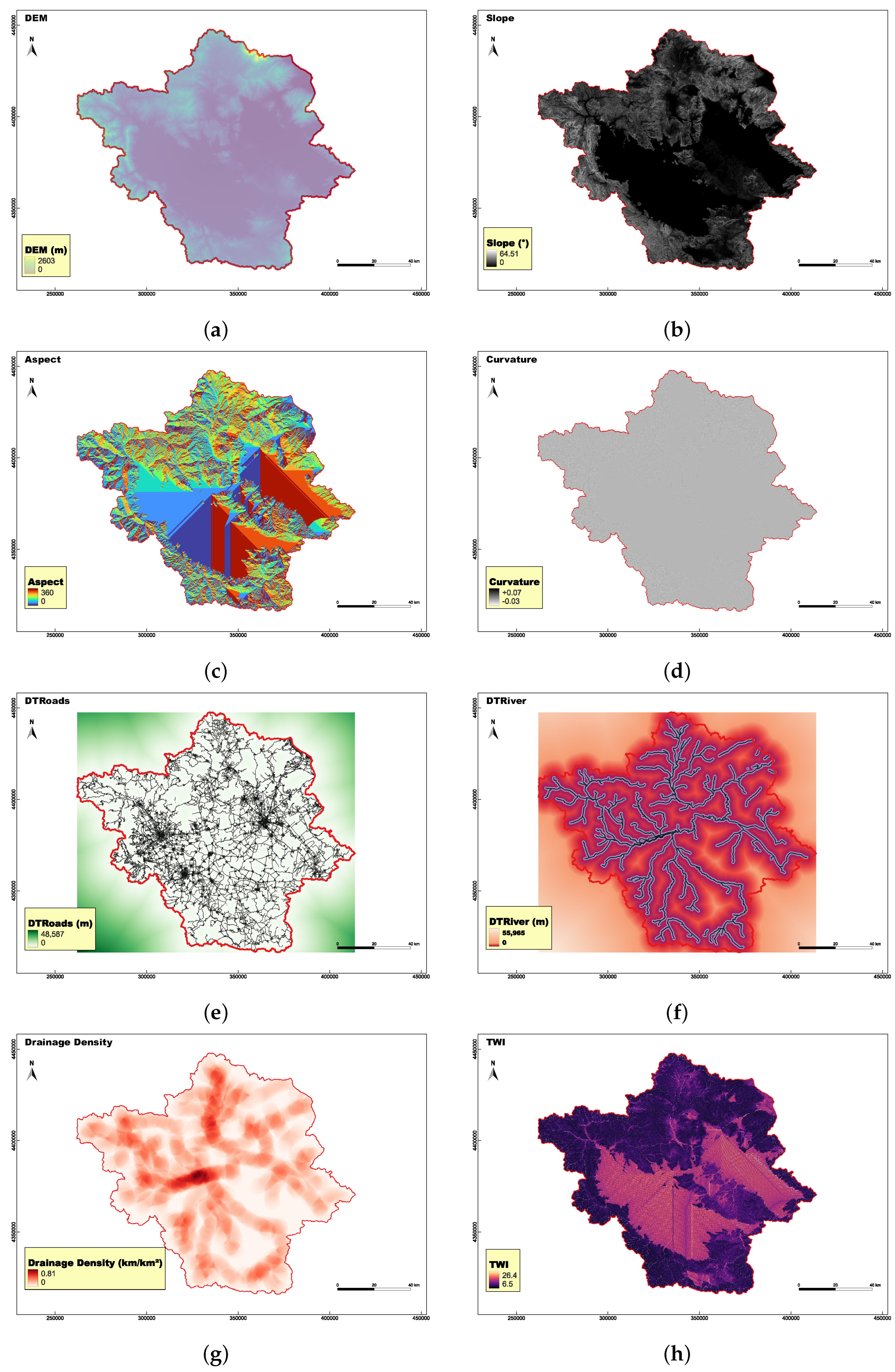
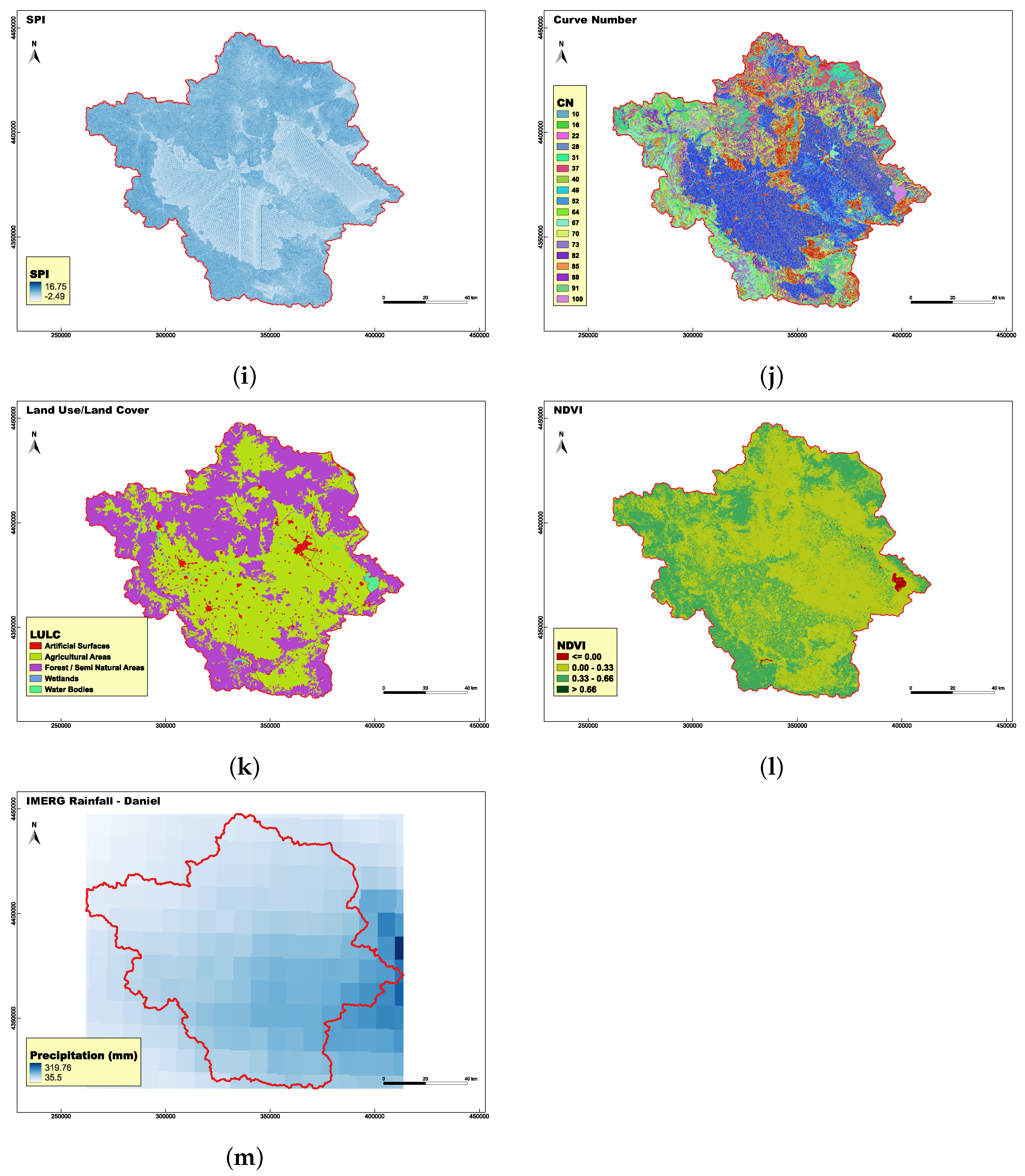
This section outlines and explains each of the factors selected and their relevance to flood. The selection of conditioning variables for flood susceptibility mapping was based on a combination of data availability, relevance to flood-generating processes, and briefly literature review from previous studies in the field. This approach guarantees the selected variables are both publicly accessible and scientifically supported. The following analysis, processing of input variables, needed calculations and mapping were conducted using tools available in QGIS 3.34.13 software. We ended up with 13 factors, i.e., digital elevation model (DEM), slope, aspect, curvature, distance from roads, distance from rivers, drainage density, topographic wetness index (TWI), stream power index (SPI), curve number (CN), land use / land cover (LULC), normalized difference vegetation index (NDVI) and rainfall. Figure presents the maps of the derived factors, while Table 3 provides a summary of their sources. All data were converted into 30×30 m grid (DEM’s grid size) for analysis if there original format differed.
Elevation, obtained from digital elevation model (DEM), is one of the most critical factors in flood susceptibility, as lower elevation areas tend to accumulate runoff and are more likely to flood during heavy rainfall events. On the other hand, high altitude facilitate faster drainage, reducing likelihood of flood occurrence. The source provides a 30×30 m size resolution, collected from [43] (Figure a).
Slope affects flood dynamics by controlling the speed and direction of surface runoff. Steeper slopes are typically promote faster water flow, reducing the potential for accumulation. Flat flows, increase likelihood of flooding. Slope angle is calculated directly from the DEM and is expressed in degrees (Figure b).
Aspect, which refers to the direction of the slope, can indirectly influence flood susceptibility by affecting variables such as frontal precipitation direction and evapotranspiration, and as a result it also affects vegetation. Aspect is calculated from DEM and contains values from 0 to 360 that express the slope direction, starting from North (0°) and continuing clockwise. (Figure c).
Curvature describe the shape of the land surface and influences how water flows across it. Curvature is calculated from DEM in QGIS environment. Positive curvature refers to concave areas, zero values to flat areas and negative values to convex areas. Thus, terrain curvature plays a key role in determining water flow patterns and flood-prone zones (Figure d).
Distance from roads (DTRoads) is a significant factor influenced by infrastructure development, as roads often disrupt natural drainage patterns and can contribute to flooding. Euclidean distance was used to determine this feature from the road network (Figure e).
Distance from rivers (DTRiver) is crucial, as areas located closer to rivers are more likely to experience flooding. Euclidean distance was used as well for this feature (Figure f).
Drainage density refers to the total length of streams and rivers per unit area and it is expressed in km/km2 (Figure g).
Topographic wetness index (TWI) is a widely used hydrological indicator that estimates the spatial distribution of moisture in a catchment. High TWI values indicate areas that are likely to be wetter, such as valleys or flat regions—often prone to flooding. TWI was calculated using the Equation 13 (Figure h).
Topographic Wetness Index (TWI) is a widely used hydrological indicator that estimates the spatial distribution of soil moisture and potential water accumulation in a landscape. is a quantitative measure of the potential for water accumulation in a landscape, based on local slope and upstream contributing area and can identify areas where water is likely to collect.
where is the specific catchment area (flow accumulation at grid cell multiplied by grid cell area and then divided by the contour width, in m2/m) and is the slope at the corresponding grid cell (in radians).
Stream power index (SPI) is a hydrological factor that quantifies the erosion flowing water based on both slope and upstream contributing area, helping to identify areas at risk of concentrated runoff and flooding. It was calculated with the Equation 14 (Figure i).
where , are as previously defined.
Curve number (CN) is a hydrologic empirical parameter for predicting direct runoff from rainfall excess. It was developed by the USDA Natural Resources Conservation Service, with the method of Soil Conservation Service (SCS) [45]. It reflects how easily rainfall turns into surface runoff in a particular area (Figure j).
Land use / land cover (LULC) map represents the physical and human-defined characteristics of the watershed surface, which significantly influence flood behavior. Five classes were identified, taking the first level of the given subdivision, i.e., Artificial Surfaces, Agricultural Areas, Forest / Semi Natural Areas, Wetlands and Water Bodies (Figure k).
Normalized difference vegetation index (NDVI) is a satellite-derived index that measures the density and health of vegetation by comparing the difference between near-infrared (NRI) light (which vegetation strongly reflects) and red light (which vegetation absorbs). Images from Sentinel 2 mission were used and the Equation 15 applied. Four classes were created (Figure l) depending on there values and that is:
- −1 - 0: dead plant
- 0 - 0.33: diseased plant
- 0.33 - 0.66: moderate healthy plant
- 0.66 - 1: very healthy plant
Rainfall is one of the most critical factors in floods, as it directly contribute to the volume and intensity of the surface runoff. In this study we used the rainfall observed by the IMERG (Integrated Multi-satellite Retrievals for GPM) obtained from Giovanni. This is a widely used dataset that combines multiple satellite observations to estimate precipitation at fine spatial and temporal scales. Since the flooded areas used in this study arise from the extreme Daniel event, it is essential to incorporate the corresponding rainfall that caused these floods. Therefore, we obtained the rainfall data at 30-minute intervals for the period of 4–7 September 2020, from IMERG and aggregated to compute the total rainfall of the event. The maximum rainfall observed by satellite inside the river basin was 250 mm (Figure m).
Table 3.
Data sources of the selected flood conditioning factors.
| Data | Source |
|---|---|
| DEM | from Copernicus GLO 30 https://dataspace.copernicus.eu/ (accessed on 15 December 2024) [43] |
| Slope | calculated from DEM |
| Aspect | calculated from DEM |
| Curvature | calculated from DEM |
| DTRoads | from OSM https://www.openstreetmap.org/ (accessed on 10 December 2024) |
| DTRiver | from GeoData http://geodata.gov.gr/ (accessed on 8 January 2025) |
| Drainage Density | from hydrographic network - GeoData http://geodata.gov.gr/ (accessed on 8 January 2025) |
| TWI | calculated from DEM |
| SPI | calculated from DEM |
| CN | calculated from slope, soil, land use [44] |
| LULC | from National Cadastre CORINE 2018 https://data.ktimatologio.gr/ (accessed on 5 January 2025) |
| NDVI | from Copernicus Sentinel 2 https://browser.dataspace.copernicus.eu/ (accessed on 5 February 2025) |
| Rainfall | from Giovanni https://giovanni.gsfc.nasa.gov/giovanni/ (accessed on 7 March 2025) |
| Flooded Area | from Copernicus Sentinel 1 https://browser.dataspace.copernicus.eu/ (accessed 10 February 2025) |
Figure 8.
Flood Conditioning factors used. (a) DEM. (b) Slope. (c) Aspect. (d) Curvature. (e) DTRoads. (f)
DTRiver. (g) Drainage Density. (h) SPI. (i) TWI. (j) CN. (k) LULC. (l) NDVI. (m) Total rainfall during Daniel storm.
Coordinate System: GGRS87/Greek Grid (EPSG:2100).
Figure 8.
Flood Conditioning factors used. (a) DEM. (b) Slope. (c) Aspect. (d) Curvature. (e) DTRoads. (f)
DTRiver. (g) Drainage Density. (h) SPI. (i) TWI. (j) CN. (k) LULC. (l) NDVI. (m) Total rainfall during Daniel storm.
Coordinate System: GGRS87/Greek Grid (EPSG:2100).
4. Analysis and Results
4.1. Problem and Model Setup
As stated in Section 3.2 the overall dataset that is used for the training and testing of the algorithms containing 3 950 grid cell points, equally divided between flooded and non-flooded instances. Each point includes the 13 independent variables that affects the flood along with a dependent variable indicating whether the location is flooded or non-flooded. We then split the data into 80% (i.e. 3 160) for the training purposes and the rest 20% (i.e. 790) for testing the models, ensuring that the ratio of flooded and non-flooded samples remained consistent across both subsets.
In order to explore and visualize the linear relationships among the flood conditioning variables in the dataset, a Pearson correlation matrix was computed. The resulting matrix, is visualized through a heatmap in Figure 9 reveals both the strength and direction of pairwise correlations. Values ranging from −1, indicating a perfect negative linear relationship, to +1, indicating a perfect positive linear relationship. Due to the fact that the highest absolute correlation coefficient is 0.7, which is below the common multicollinearity threshold of 0.8 [46], we proceeded with including all features in the training set. We also experimented with removing the variables showing the highest correlations, but this had no noticeable impact on models’ performance, so all features were retained.
To ensure robust model performance, cross-validation was employed during the evaluation process. Each model used in this study was trained using 5-fold cross-validation to mitigate overfitting and accuracy as scoring metric. In this approach, the dataset is divided into five equal parts; in each iteration, four parts are used for training and the remaining one for validation, rotating until every subset has been used for validation once. Following hyperparameter optimization using Grid Search, the finalized parameter values of models are presented in Table 4. All analyses and code implementation were carried out using Python 3.11.12 with relevant scientific libraries, e.g. XGBoost Python package 2.1.4 and scikit-learn 1.6.1 version. Model training was performed on Google Colab, utilizing an Intel Xeon CPU with 2 vCPUs (virtual CPUs) and 13 GiB of RAM, to provide a suitable computational environment for machine learning tasks.
4.2. Results and Comparison
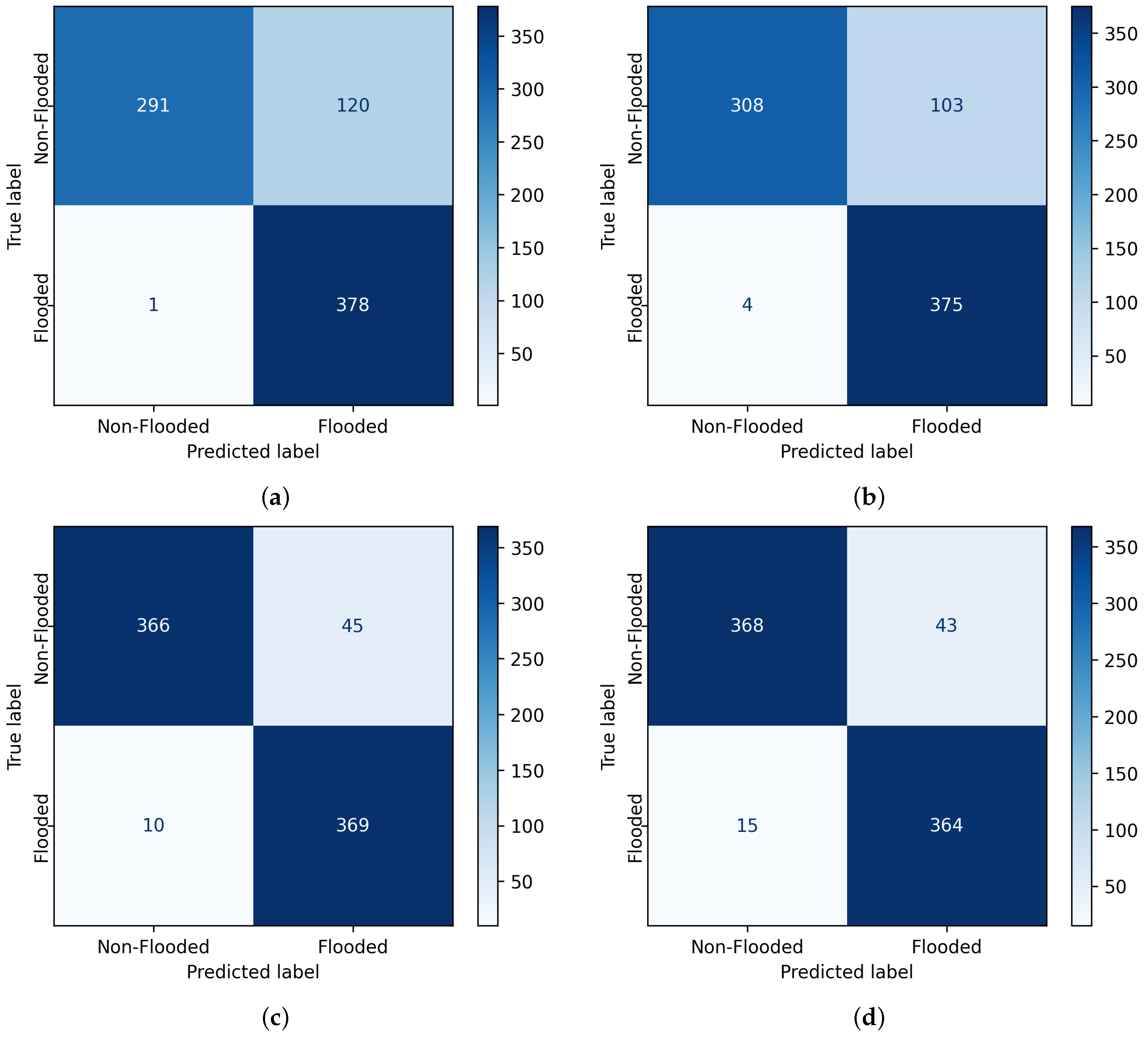
With the models being trained, we evaluate their performance on the testing set. A comparison of confusion matrices for the different models is demonstrated in Figure 10. The format of the illustrated matrix is as follows:
Both Logistic Regression (LR) and Support Vector Machine (SVM) yield a high value of false positives, which means that they predict that the point is flooded when it is actually not. Random Forest (RF) and eXtreme Gradient Boosting (XGBoost) minimize the false positive and negative values, misclassifying only 55 and 58 samples respectively, out of 790 total testing samples (cells).
Table 5 summarizes the values of the five metrics, i.e., accuracy, precision, recall, specificity and . For each evaluation metric the highest scores are emphasized in bold. As shown in the table the tree-based models (i.e., Random Forest and Extreme Gradient Boosting) demonstrate superior performance in general, achieving consistently high results across all metrics. Furthermore, Figure 11 presents the Receiver Operating Characteristic (ROC) curves and the corresponding Area Under the Curve (AUC). The ROC curve shows the trade-off between sensitivity (or TPR) and 1 − specificity (or FPR). Dotted lines represent ideal classifier (top-left curve) and random classifier (the diagonal where FPR = TPR). Curves that approach the perfect classifier indicate better performance, whereas on the contrary those closer to random line suggests weaker or poor performance. Aside from visual inspection, which can be critical in some cases, a measure that summarize the performance of each classifier is needed in order to compare different models. AUC score measures the area under the ROC curve and gives a general predictive score. From Figure 11, it can be observed that LR performs worse than the other models. SVM performs slightly better, while the tree-based models (RF and XGBoost) show the best performance with similar ROC curves—occasionally, one slightly surpasses the other. Quantitatively, RF performs the best AUC score of 0.969, slightly outperforming XGBoost (AUC = 0.968). This improved performance can be attributed to their ability to capture complex, non-linear relationships and interactions within the data, which simpler models may fail to detect.
4.3. FSM Maps
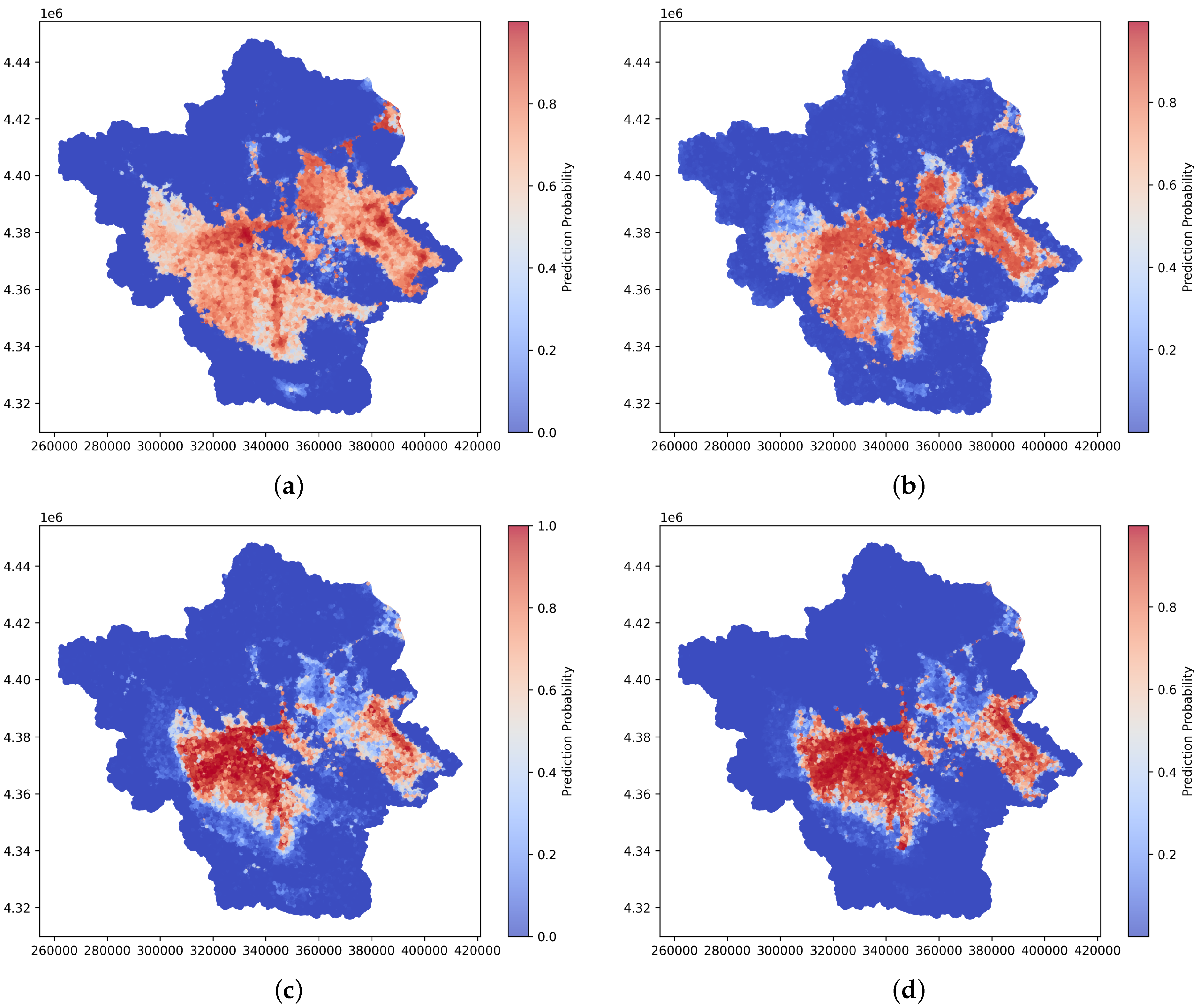
It is important to have a flood susceptibility map for the complete watershed, when an extreme events like the Daniel storm taking place. Hence, Figure 12 depicts the flood susceptibility maps generated by each of the models applied, indicating the probability of flooding for each cell. LR and SVM predict significantly larger flood-prone areas compared to RF and XGBoost, which identify more limited regions as susceptible to flooding. According to tree-based models, which demonstrated superior performance, the most flood-prone areas are located in the eastern region and the central to southern region, as highlighted in red.
4.4. Feature Importance
As mentioned in Section 2.5 feature importance allows you to understand the relationship between the features and the target output. In that manner, it is distinguished what feature is the most effective for the model. As Random Forest performed the best out of evaluation assessment, with respect to ROC curve and AUC score, it was selected as the primary model for further analysis and investigation. To measure how each feature is influencing the output in RF, we used Mean Decrease in Impurity (MDI) (Figure 13a) and permutation-based (Figure 13b). Both methods suggest that the most influential factors in the RF model is DEM, slope, rainfall and TWI. The DEM, slope and TWI variables are critical as they directly influence the topographic characteristics of the landscape, which are crucial in flood modeling. Additionally, rainfall provide important environmental context, representing precipitation patterns.
4.5. Initial Data Experimentation
With the intention of verifying the generalizability of the model and evaluate the potential impact of the initial training data selection, we conducted two additional experiments. In each experiment, the Peneus watershed was divided into two halves. For the first experiment, 3 950 training data points were sampled exclusively from the eastern half, while in the second, the same number of points was selected from the western half. After training the RF model in both datasets, two trained models were developed. FSM for the entire basin were generated, and the results are presented in Figure 14. As we can observe, the training data have some influence on the resulting FSM. To quantify and compare the results we produced the ROC and AUPRC (Area Under Precision-Recall) curve in Figure 15 for the 3 models, i.e., trained with points from the whole basin, trained with points from the right-half basin and trained from the left-half basin. Not unexpectedly, the model trained using data points from the entire basin—thus capturing spatial variability across the full study area—exhibited better performance compared to those trained on spatially limited subsets. Nevertheless, the accuracy of models’ remains at a high level.
4.6. FSM for T=1000-Year Rainfall Scenario
Flood susceptibility maps are essential for identifying high-risk areas and guiding flood mitigation and land-use planning efforts, in the area. Inference in machine learning, refer to the process of applying a trained model to new data in order to generate predictions. Under these circumstances we constructed a FSM referring to a 1000-year return period rainfall scenario at 24 h scale. The new methodological stochastic framework for the construction of rainfall intensity–time scale–return period relationships [47] (referred as ombrian curves), was adopted. This approach was applied recently within Greek territory [48,49]. The relationship between the rainfall intensity x to any timescale k and return period T is given by the Equation 16:
where five parameters are essential, i.e., an intensity scale parameter in units of x (e.g. mm/h), a timescale parameter in units of the return period (e.g., years), a timescale parameter in units of timescale (e.g., h) with , a dimensionless parameter with , the tail index of the process. The total precipitation level can be determined by multiplying the rainfall intensity x with the corresponding timescale (i.e. 24 h). Figure 16 shows the rainfall distribution across the study area. The corresponding FSM is depicted in Figure 17, highlighting three main classes: low, moderate, and high flood susceptibility zones.
5. Discussion and Future Research Directions
In recent years, machine learning techniques have been used to to map flood susceptibility across many regions globally. They are highly effective in flood susceptibility mapping because of their ability to leverage historical flood data to uncover hidden patterns in environmental data. Here, we highlight how these models can be leveraged to make more accurate, data-driven predictions. However, despite the growing popularity, their application still remains relatively underdeveloped, and there is still significant room for improvement. In the present, we applied machine learning algorithms for the creation of flood susceptibility maps in the region of Thessaly, aiming to enhance flood protection of the area and provide more insights into the applied methodology. We utilized satellite-derived data to access flooded areas from a massive recent extreme event, i.e., Daniel Storm, along with the corresponding satellite-based rainfall of the event.
We created a dataset of 3 950 data points consisting of 13 flood conditioning factors as independent variables and corresponding binary flood labels. Factors included dem, slope, aspect, Curvature, distance from roads, distance from rivers, drainage density, topographic wetness index, stream power index, curve number, land use, normalized difference vegetation index and rainfall. As we divide the balanced dataset into 80% for train and the rest 20% for test, we compared the performance of LR, SVM, RF and XGBoost in a classification procedure. In this performance assessment through various metrics, like accuracy, precision, recall, specificity, F1 score, and ROC curve, the tree-based algorithms performed better achieving a Area Under the Curve (AUC) score of 0.97, with 1.0 representing the highest possible score. Feature importance of RF revealed that terrain variables, such as DEM, slope and TWI along with the event’s rainfall, are the most significant contributors.
To investigate the generalizability of the model and assess the impact of the initial training data, we conducted additional experiments. As we divided the catchment into half, we use data from one side each time to train a random forest model. The results highlight the model’s sensitivity to the training data, suggesting that generalizability may be influenced by spatial characteristics. This finding highlights the need for caution when applying the model to new areas with different spatial features. To improve generalizability, it may be necessary to incorporate diverse data sources or ensure a more representative distribution of training data that covers a broader range of spatial conditions.
Flood early warning systems are critical tools for disaster risk reduction, enabling timely alerts and proactive measures to minimize damage and protect communities at risk [50]. The proposed approach can also serve as an early warning system, wherein a pre-trained model operates for a real-time rainfall forecast to identify areas likely to be most affected by the event. This method could complement or even replace time-consuming simulations traditionally conducted with conventional hydraulic models. Such a scenario was included in the study, in which a map based on 1000-year return period rainfall event was generated, and the susceptible areas were identified. This scenario was made using the updated parameters of the ombrian curves in Greece, within the implementation of the EU Directive 2007/60/EC [49]. A trained model required less than 5 min to produce the outputs. The resulted map showing two major zones of high flood susceptibility inside the basin, specifically in the eastern and central-to-southern regions, highlighting the need for targeted measures and actions.
As civil engineers, we are driven by our training and desire to provide decision-makers with information about the solution for every situation, regardless of the challenges involved. It is important to not attribute failure to unforeseen events and unrealistic theories. Anticipating and mitigating potential risks, can greatly reduce the aftermath of the resulting consequences, all civil protection guidance highlight the importance and added values of anticipatory planning and design in disaster management. Our case study area, Thessaly, has been suffering from both flooding and lack of water for many years, yet the responses have proven insufficient in many cases. Solutions can only be achieved through civil engineering works and infrastructure designed to mitigate these challenges, still the responsible authorities and sometimes the wider community, often resist the implementation of these projects. A robust strategic plan could investigate if and how multipurpose dams all around the PRB, which may combine storing and supplying water for irrigation, industry and human consumption with other uses such as flood control and hydroelectric power generation, can help the area. These infrastructure projects, properly studied, are among the most effective ways to prevent flooding and their landscape design is beneficial for the landscape quality perception as well as the touristic development [51].
Although the integration of satellite data with machine learning shows great potential for flood susceptibility analysis, several challenges remain to be addressed. Firstly limited spatial and temporal resolution of satellite imagery and high-quality satellite data may not be available in the specific period. SAR images often contain noise, which can reduce the accuracy of flood detection and require complex preprocessing [52]. Moreover, the rainfall data derived from satellite observations may not always be accurate and can sometimes diverge from the ground truth measurements [53]. Accurate ground truth data labeling for training machine learning model can be challenging in some regions. ML models trained on a specific region may not generalize well to other areas. In addition, processing high-resolution satellite data may require significant computational resources.
This study can serve as a foundation for future research, that can build upon it to explore potential improvements to the methods used in the current work. To begin with, not only point-based models (SVM, RF etc.), but an image-based models like Convolutional Neural Networks (CNNs) can be adopted. The main benefit from such a model is that it can capture spatial patterns and information as pixels of the image are not treated independently. Additionally, more historical flood events could be considered; but, in that case the feature of rainfall should be adopted by accounting for all precipitation that contributed to those events. It is also worth noting that a key question to address is how many data samples are necessary to consider the ML model accurate. Another important aspect is the reliable quantification of the uncertainty of each model. One way to accomplish this is via the BlueCat [54] approach, which operates by transforming a point prediction provided by a model to a corresponding stochastic formulation. While conventional ML models ignore any underlying physical law certain types of neural networks, such as Physics-Informed Neural Networks (PINNs) [55] and Neural Operators [56], which fall under the broader domain of Scientific Machine Learning, are specifically designed to incorporate them into the modeling process. PINNs solve partial differential equations (PDEs) by embedding physical laws into neural networks, while neural operators learn mappings between function spaces to rapidly approximate solutions to complex systems. These could be useful, as flood modeling typically employs the shallow water equations or the Navier-Stokes equations. Lastly, but equally important, is the growing effort to interpret how some machine learning models function (Interpretable AI [57]) and provide clear explanations for their outputs and help decision making processes (Explainable AI [58]). It is important to understand the reasoning behind the the prediction of each model, regardless of its complexity.
6. Summary and Conclusions
Our research focuses on the contribution of machine learning algorithms to the flood susceptibility mapping. Using 13 flood conditioning factors and satellite data, we trained four models on a classification task in our case study area Peneus basin. The performance of Logistic Regression (LR), Support Vector Machine (SVM), Random Forest (RF) and eXtreme Gradient Boosting (XGBoost) was compared using standard evaluation indicators. Feature importance was analyzed for the best-performing model (RF). To assess the generalizability, the RF model was trained using different subsets of data by splitting the basin in half. Finally, a rainfall scenario for 1000-year return period with at 24-hour scale was developed to support long-term flood risk assessment and planning. Based on the analysis and evaluation of the applications, the key findings are outlined below:
- Tree-based models, particularly RF and XGBoost, outperformed the other algorithms, achieving the highest Area Under the Curve AUC scores—RF: 0.969, XGBoost: 0.968, SVM: 0.940, LR: 0.907.
- Feature importance analysis revealed the most influential factors contributing to flood susceptibility in decreasing order is DEM, slope, rainfall and TWI, providing valuable insights for model interpretation and decision-making.
- The choice of initial training data impacts model performance and generalizability, highlighting the need for careful dataset selection in spatial prediction tasks.
- The identified areas with high flood susceptibility is the eastern and the central-to-southern regions, offering useful information for targeted risk mitigation and planning efforts.
- Machine learning algorithms offer a promising approach for flood susceptibility mapping and can be extended as an early warning system, requiring significantly less time compared to traditional models.
Floods continue to be a major socio-environmental challenge, causing widespread damage and disruption. While accurate FSMs are essential for effective flood risk management and preparedness, this remains a complex task due to the variability of climatic, hydrological, and geographical factors. Machine learning offers a promising avenue for improving predictive capabilities by leveraging data-driven insights. However, ongoing research is needed to enhance model robustness, generalizability, and integration into real-time early warning systems. Ultimately, the integration of domain knowledge with advanced technologies offer powerful solutions for developing effective flood control strategies.
Author Contributions
Conceptualization, N.T., I.B., D.K.; methodology, N.T.; software, N.T.; validation, N.T.; formal analysis, N.T.; investigation, N.T., I.B., D.K, T.I. and P.D.; resources, N.T.; data curation, N.T., I.B.; writing—original draft preparation, N.T.; writing—review and editing, N.T., I.B and D.K.; visualization, N.T.; supervision, N.T., I.B., D.K., T.I. and P.D.; project administration, N.T., I.B., D.K., T.I. and P.D. All authors have read and agreed to the published version of the manuscript.
Funding
This research received no external funding. N.T. received partial support through a scholarship from the Special Account for Research Funding (E.L.K.E) of National Technical University of Athens.
Data Availability Statement
Data collected from various sources. All data used in the study are freely available from public sources. Detailed descriptions of the datasets and their respective sources are provided in the corresponding sections of the manuscript.
Conflicts of Interest
The authors declare no conflict of interest.
References
- Jonkman, S. N. Global Perspectives on Loss of Human Life Caused by Floods. Natural Hazards 2005, 34, 151–175. [Google Scholar] [CrossRef]
- Yu, Q.; Wang, Y.; Li, N. Extreme Flood Disasters: Comprehensive Impact and Assessment. Water 2022, 14, 1211. [Google Scholar] [CrossRef]
- European Commission. Directive 2007/60/EC of the European Parliament and of the Council of 23 October 2007 on the Assessment and Management of Flood Risks; L 288, 6.11.2007; Official Journal of the European Communities: Aberdeen, UK, 2007; p. 27. [Google Scholar]
- Bentivoglio, R.; Isufi, E.; Jonkman, S. N.; Taormina, R. Deep learning methods for flood mapping: a review of existing applications and future research directions. Hydrology and Earth System Sciences 2022, 26, 4345–4378. [Google Scholar] [CrossRef]
- Avila-Aceves, E.; Wenseslao Plata-Rocha; Sergio Alberto Monjardin-Armenta; Jesús Gabriel Rangel-Peraza. Geospatial modelling of floods: a literature review. Stochastic environmental research and risk assessment 2023, 37, 4109–4128. [Google Scholar] [CrossRef]
- Abdullah, M.F.; Siraj, S.; Hodgett, R.E. An Overview of Multi-Criteria Decision Analysis (MCDA) Application in Managing Water-Related Disaster Events: Analyzing 20 Years of Literature for Flood and Drought Events. Water 2021, 13, 1358. [Google Scholar] [CrossRef]
- Liuzzo, L.; Sammartano, V.; Freni, G. Comparison between Different Distributed Methods for Flood Susceptibility Mapping. Water Resources Management 2019, 33, 3155–3173. [Google Scholar] [CrossRef]
- Chen, H.; Yang, D.; Hong, Y.; Gourley, J. J.; Zhang, Y. Hydrological data assimilation with the Ensemble Square-Root-Filter: Use of streamflow observations to update model states for real-time flash flood forecasting. Advances in Water Resources 2013, 59, 209–220. [Google Scholar] [CrossRef]
- Soomro, S.; Hu, C.; Muhammad Waseem Boota; Ahmed, Z. ; Liu Chengshuai; Zhenyue, H.; Xiang, L.; Hyder, M. River Flood Susceptibility and Basin Maturity Analyzed Using a Coupled Approach of Geo-morphometric Parameters and SWAT Model. Water Resources Management 2022, 36, 2131–2160. [Google Scholar] [CrossRef]
- Stoleriu, C. C.; Urzica, A.; Mihu-Pintilie, A. Improving flood risk map accuracy using high-density LiDAR data and the HEC-RAS river analysis system: A case study from north-eastern Romania. Journal of Flood Risk Management 2020, 13, e12572. [Google Scholar] [CrossRef]
- Wahba, M.; Sharaan, M.; Elsadek, W.M.; Kanae, S.; Hassan, H.S. Examination of the efficacy of machine learning approaches in the generation of flood susceptibility maps. Environ. Earth Sci. 2024, 83, 429. [Google Scholar] [CrossRef]
- Seleem, O.; Ayzel, G.; de Souza, A.C.T.; Bronstert, A.; Heistermann, M. Towards urban flood susceptibility mapping using data-driven models in Berlin, Germany. Geomat. Nat. Hazards Risk 2022, 13, 1640–1662. [Google Scholar] [CrossRef]
- Saravanan, S.; Abijith, D.; Reddy, N.M.; KSS, P.; Janardhanam, N.; Sathiyamurthi, S.; Sivakumar, V. Flood susceptibility mapping using machine learning boosting algorithms techniques in Idukki district of Kerala India. Urban Clim. 2023, 49, 101503. [Google Scholar] [CrossRef]
- Wedajo, G.K.; Lemma, T.D.; Fufa, T.; Gamba, P. Integrating Satellite Images and Machine Learning for Flood Prediction and Susceptibility Mapping for the Case of Amibara, Awash Basin, Ethiopia. Remote Sens. 2024, 16, 2163. [Google Scholar] [CrossRef]
- Kourgialis, N.N.; Karatzas, G.P. A national scale flood hazard mapping methodology: The case of Greece—Protection and adaptation policy approaches. Sci. Total Environ. 2017, 601–602, 441–452. [Google Scholar] [CrossRef] [PubMed]
- Tsinidis, G.; Koutas, L. Geotechnical and Structural Damage to the Built Environment of Thessaly Region, Greece, Caused by the 2023 Storm Daniel. Geotechnics 2025, 5, 16. [Google Scholar] [CrossRef]
- Dimitriou, E.; Efstratiadis, A.; Zotou, I.; Papadopoulos, A.; Iliopoulou, T.; Sakki, G.-K.; Mazi, K.; Rozos, E.; Koukouvinos, A.; Koussis, A.D.; et al. Post-Analysis of Daniel Extreme Flood Event in Thessaly, Central Greece: Practical Lessons and the Value of State-of-the-Art Water-Monitoring Networks. Water 2024, 16, 980. [Google Scholar] [CrossRef]
- Sreekala, S.; Geetha, P.; Madhu, D. Flood Susceptibility Map of Periyar River Basin Using Geo-Spatial Technology and Machine Learning Approach. Remote Sensing in Earth Systems Sciences. 2024, 8, 1–21. [Google Scholar] [CrossRef]
- Al-Ruzouq, R.; Shanableh, A.; Jena, R.; Gibril, M.B.A.; Hammouri, N.A.; Lamghari, F. Flood susceptibility mapping using a novel integration of multi-temporal sentinel-1 data and eXtreme deep learning model. Geosci. Front. 2024, 15, 101780. [Google Scholar] [CrossRef]
- Nachappa, T.G.; Piralilou, S.T.; Gholamnia, K.; Ghorbanzadeh, O.; Rahmati, O.; Blaschke, T. Flood susceptibility mapping with machine learning, multi-criteria decision analysis and ensemble using Dempster Shafer Theory. J. Hydrol. 2020, 590, 125275. [Google Scholar] [CrossRef]
- Hitouri, S.; Mohajane, M.; Lahsaini, M.; Ali, S.A.; Setargie, T.A.; Tripathi, G.; D’antonio, P.; Singh, S.K.; Varasano, A. Flood Susceptibility Mapping Using SAR Data and Machine Learning Algorithms in a Small Watershed in Northwestern Morocco. Remote Sens. 2024, 16, 858. [Google Scholar] [CrossRef]
- Seydi, S.T.; Kanani-Sadat, Y.; Hasanlou, M.; Sahraei, R.; Chanussot, J.; Amani, M. Comparison of Machine Learning Algorithms for Flood Susceptibility Mapping. Remote Sens. 2023, 15, 192. [Google Scholar] [CrossRef]
- Al-Kindi, K. M.; Alabri. , z. Investigating the Role of the Key Conditioning Factors in Flood Susceptibility Mapping through Machine Learning Approaches. Earth Syst. Environ. 2024, 8, 63–81. [Google Scholar] [CrossRef]
- Shafizadeh-Moghadam, H.; Valavi, R.; Shahabi, H.; Chapi, K.; Shirzadi, A. Novel forecasting approaches using combination of machine learning and statistical models for flood susceptibility mapping. J. Environ. Manag. 2018, 217, 1–11. [Google Scholar] [CrossRef] [PubMed]
- Cox, D. R. The Regression Analysis of Binary Sequences. Journal of the Royal Statistical Society: Series B (Methodological) 1958, 20, 215–232. [Google Scholar] [CrossRef]
- Myung, I. J. Tutorial on Maximum Likelihood Estimation. Journal of Mathematical Psychology 2003, 47, 90–100. [Google Scholar] [CrossRef]
- Boser, B. E.; Guyon, I. M.; Vapnik, V. N. A Training Algorithm for Optimal Margin Classifiers. Proceedings of the Fifth Annual Workshop on Computational Learning Theory 1992. [Google Scholar] [CrossRef]
- Schölkopf, B. The Kernel Trick for Distances. In Proceedings of the 13th International Conference on Neural Information Processing Systems (NIPS’00), Hong Kong, China, 3–6 October 2006; MIT Press: Cambridge, MA, USA, 2000; pp. 283–289. [Google Scholar]
- Breiman, L. Random forests. Mach. Learn. 2001, 45, 5–32. [Google Scholar] [CrossRef]
- Quinlan, J.R. Induction of decision trees. Mach. Learn. 1986, 1, 81–106. [Google Scholar] [CrossRef]
- Chen, T.; Guestrin, C. XGBoost: A Scalable Tree Boosting System. In Proceedings of the 22nd ACM SIGKDD International Conference on Knowledge Discovery and Data Mining (KDD ’16), San Francisco, CA, USA, 13–17 August 2016; pp. 784–794. [Google Scholar]
- Kaggle Competitions. Available online: https://www.kaggle.com/competitions (accessed on 24 September 2024).
- Amjad, M.; Ahmad, I.; Ahmad, M.; Wróblewski, P.; Kamiński, P.; Amjad, U. Prediction of Pile Bearing Capacity Using XGBoost Algorithm: Modeling and Performance Evaluation. Appl. Sci. 2022, 12, 2126. [Google Scholar] [CrossRef]
- Rengasamy, D.; Mase, J. M.; Kumar, A.; Rothwell, B.; Torres, M. T.; Alexander, M. R.; Winkler, D. A.; Figueredo, G. P. Feature importance in machine learning models: A fuzzy information fusion approach. Neurocomputing 2022, 511, 163–174. [Google Scholar] [CrossRef]
- Vatsal. Feature Importance in Machine Learning, Explained. Towards Data Science. Available online: https://towardsdatascience.com/feature-importance-in-machine-learning-explained-443e35b1b284/ (accessed on 20 April 2025).
- Tangirala, S. Evaluating the Impact of GINI Index and Information Gain on Classification Using Decision Tree Classifier Algorithm. Int. J. Adv. Comput. Sci. Appl. 2020, 11. [Google Scholar] [CrossRef]
- Lundberg, S.M.; Lee, S.I. A unified approach to interpreting model predictions. Adv. Neural Inf. Process. Syst. 2017, 30, 4765–4774. [Google Scholar]
- D’Agostino, A.; The Explanation You Need on Binary Classification Metrics. Medium. Available online: https://medium.com/data-science/the-explanation-you-need-on-binary-classification-metrics-321d280b590f (accessed on 25 April 2025).
- Iliopoulou, T.; Malamos, N.; Koutsoyiannis, D. Regional Ombrian Curves: Design Rainfall Estimation for a Spatially Diverse Rainfall Regime. Hydrology 2022, 9, 67. [Google Scholar] [CrossRef]
- Mimikou, M.; Koutsoyiannis, D. Extreme floods in Greece: The case of 1994. In Proceedings of the US-ITALY Research Workshop on the Hydrometeorology, Impacts, and Management of Extreme Floods, Perugia, Italy, 13–17 November 1995. [Google Scholar]
- Bathrellos, G.D.; Skilodimou, H.D.; Soukis, K.; Koskeridou, E. Temporal and Spatial Analysis of Flood Occurrences in the Drainage Basin of Pinios River (Thessaly, Central Greece). Land 2018, 7, 106. [Google Scholar] [CrossRef]
- Valkaniotis, S.; Papathanassiou, G.; Marinos, V.; Saroglou, C.; Zekkos, D.; Kallimogiannis, V.; Karantanellis, E.; Farmakis, I.; Zalachoris, G.; Manousakis, J.; et al. Landslides Triggered by Medicane Ianos in Greece, September 2020: Rapid Satellite Mapping and Field Survey. Appl. Sci. 2022, 12, 12443. [Google Scholar] [CrossRef]
- Copernicus DEM, 2022. Available online: https://doi.org/10.5270/esa-c5d3d65 (accessed on 15 December 2024).
- Efstratiadis, A.; Koukouvinos, A.; Michaelidi, E.; Galiouna, E.; Tzouka, K.; Koussis, A.D.; Mamassis, N.; Koutsoyiannis, D. Description of Regional Approaches for the Estimation of Characteristic Hydrological Quantities, DEUCALION—Assessment of Flood Flows in Greece under Conditions of Hydroclimatic Variability: Development of Physically-Established Conceptual-Probabilistic; Department of Water Resources and Environmental Engineering—National Technical University of Athens, National Observatory of Athens: Athens, Greece, 2014. [Google Scholar]
- USDA. Hydrology. In National Engineering Handbook; United States Department of Agriculture, Soil Conservation Service, US Government Printing Office: Washington, DC, USA, 1972. [Google Scholar]
- Grewal, R.; Cote, J.A.; Baumgartner, H. Multicollinearity and measurement error in structural equation models: Implications for theory testing. Mark. Sci. 2004, 23, 519–529. [Google Scholar] [CrossRef]
- Koutsoyiannis, D.; Iliopoulou, T.; Koukouvinos, A.; Malamos, N. A stochastic framework for rainfall intensity-time scale-return period relationships. Part I: theory and estimation strategies. Hydrological Sciences Journal 2024, 69, 1082–1091. [Google Scholar] [CrossRef]
- Iliopoulou, T.; Koutsoyiannis, D.; Malamos, N.; Koukouvinos, A.; Dimitriadis, P.; Mamassis, N.; Tepetidis, N.; Markantonis, D. A stochastic framework for rainfall intensity-time scale-return period relationships. Part II: point modelling and regionalization over Greece. Hydrological Sciences Journal 2024, 69, 1092–1112. [Google Scholar] [CrossRef]
- Koutsoyiannis, D.; Iliopoulou, T.; Koukouvinos, A.; Malamos, N.; Mamassis, N.; Dimitriadis, P.; Tepetidis, N.; Markantonis, D. [Technical Report; in Greek]. Production of Maps with Updated Parameters of the Ombrian Curves at Country Level (Implementation of the EU Directive 2007/60/EC in Greece); Department of Water Resources and Environmental Engineering—National Technical University of Athens: Athens, Greece, 2023; Available online: https://www.itia.ntua.gr/2273/ (accessed on 20 April 2025).
- Perera, D.; Seidou, O.; Agnihotri, J.; Rasmy, M.; Smakhtin, V.; Coulibaly, P.; Mehmood, H. Flood Early Warning Systems: A Review of Benefits, Challenges and Prospects; United Nations University-Institute for Water, Environment and Health: Hamilton, ON, Canada, 2019; Available online: https://inweh.unu.edu/flood-early-warning-systems-a-review-of-benefits-challenges-and-prospects/ (accessed on 15 April 2025)ISBN 978-92-808-6096-2.
- Ioannidis, R.; Sargentis, G.-F.; Koutsoyiannis, D. Landscape design in infrastructure projects - is it an extravagance? A cost-benefit investigation of practices in dams. Landsc. Res. 2022, 47, 370–387. [Google Scholar] [CrossRef]
- Singh, P.; Diwakar, M.; Shankar, A.; Shree, R.; Kumar, M. A review on SAR image and its despeckling. Arch. Comput. Methods Eng. 2021, 28, 4633–4653. [Google Scholar] [CrossRef]
- Yan, J.; Gebremichael, M. Estimating actual rainfall from satellite rainfall products. Atmos. Res. 2009, 92, 481–488. [Google Scholar] [CrossRef]
- Koutsoyiannis, D.; Montanari, A. Bluecat: A Local Uncertainty Estimator for Deterministic Simulations and Predictions. Water Resour. Res. 2022, 58. [Google Scholar] [CrossRef]
- Cuomo, S.; Di Cola, V. S.; Giampaolo, F.; Rozza, G.; Raissi, M.; Piccialli, F. Scientific Machine Learning through Physics-Informed Neural Networks: Where We Are and What’s Next. J. Sci. Comput. 2022, 92. [Google Scholar] [CrossRef]
- Li, Z.; Kovachki, N.; Azizzadenesheli, K.; Liu, B.; Bhattacharya, K.; Stuart, A.; Anandkumar, A. Fourier Neural Operator for Parametric Partial Differential Equations. In Proceedings of the International Conference on Learning Representations (ICLR), Virtual Event. 3–7 May 2021. [Google Scholar]
- Dikshit, A.; Pradhan, B. Interpretable and explainable AI (XAI) model for spatial drought prediction. Sci. Total Environ. 2021, 801, 149797. [Google Scholar] [CrossRef]
- Linardatos, P.; Papastefanopoulos, V.; Kotsiantis, S. Explainable AI: A Review of Machine Learning Interpretability Methods. Entropy 2020, 23, 18. [Google Scholar] [CrossRef]
Figure 1.
Flood Susceptibility Mapping Flowchart.
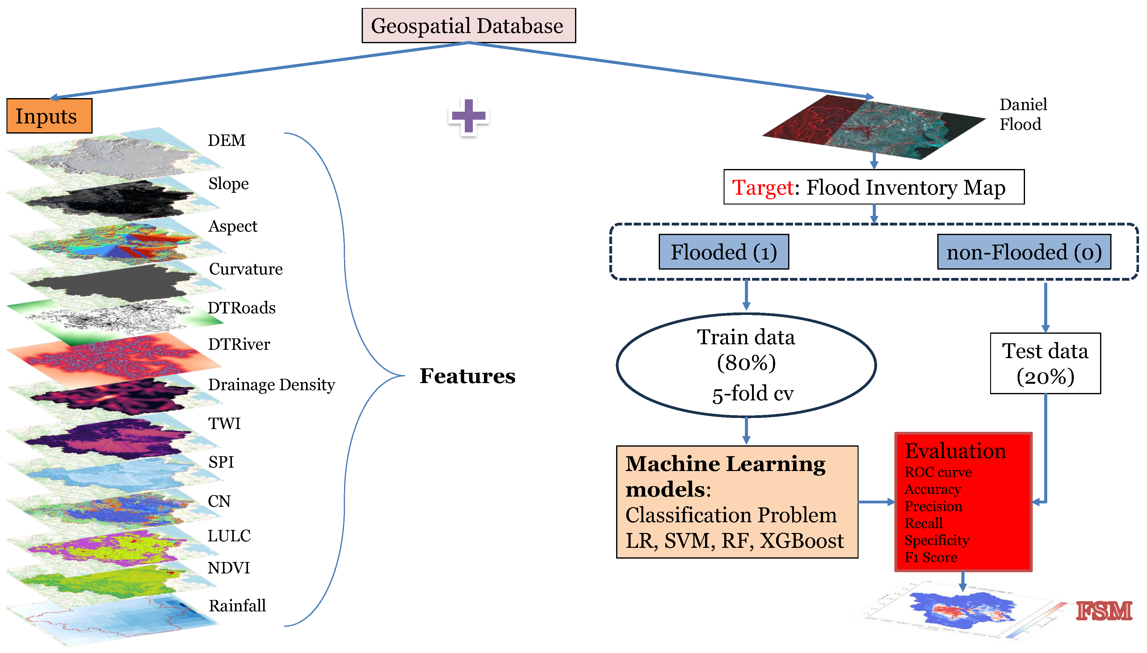
Figure 2.
Logistic Regression model.
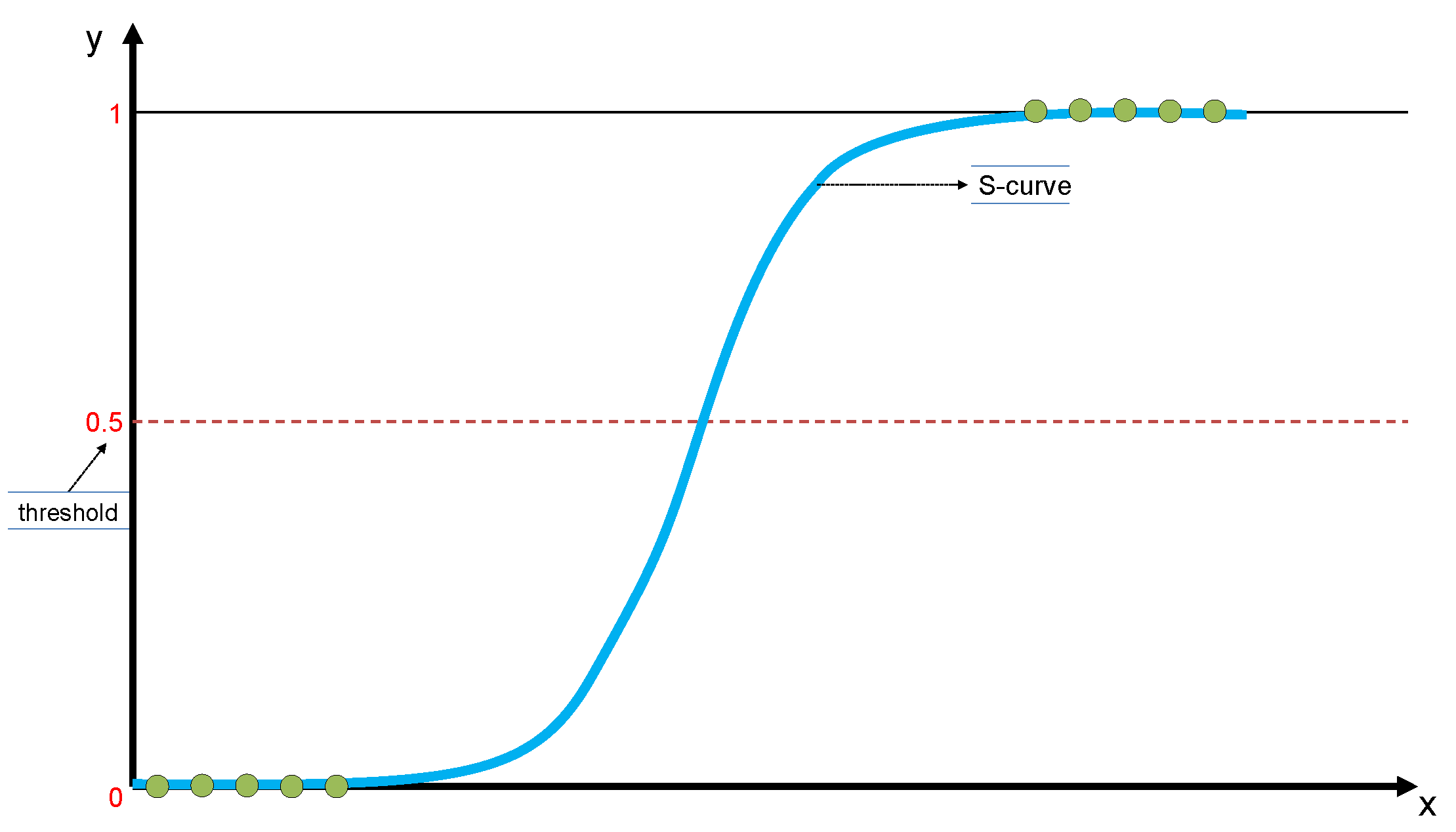
Figure 3.
Support Vector Machine model.
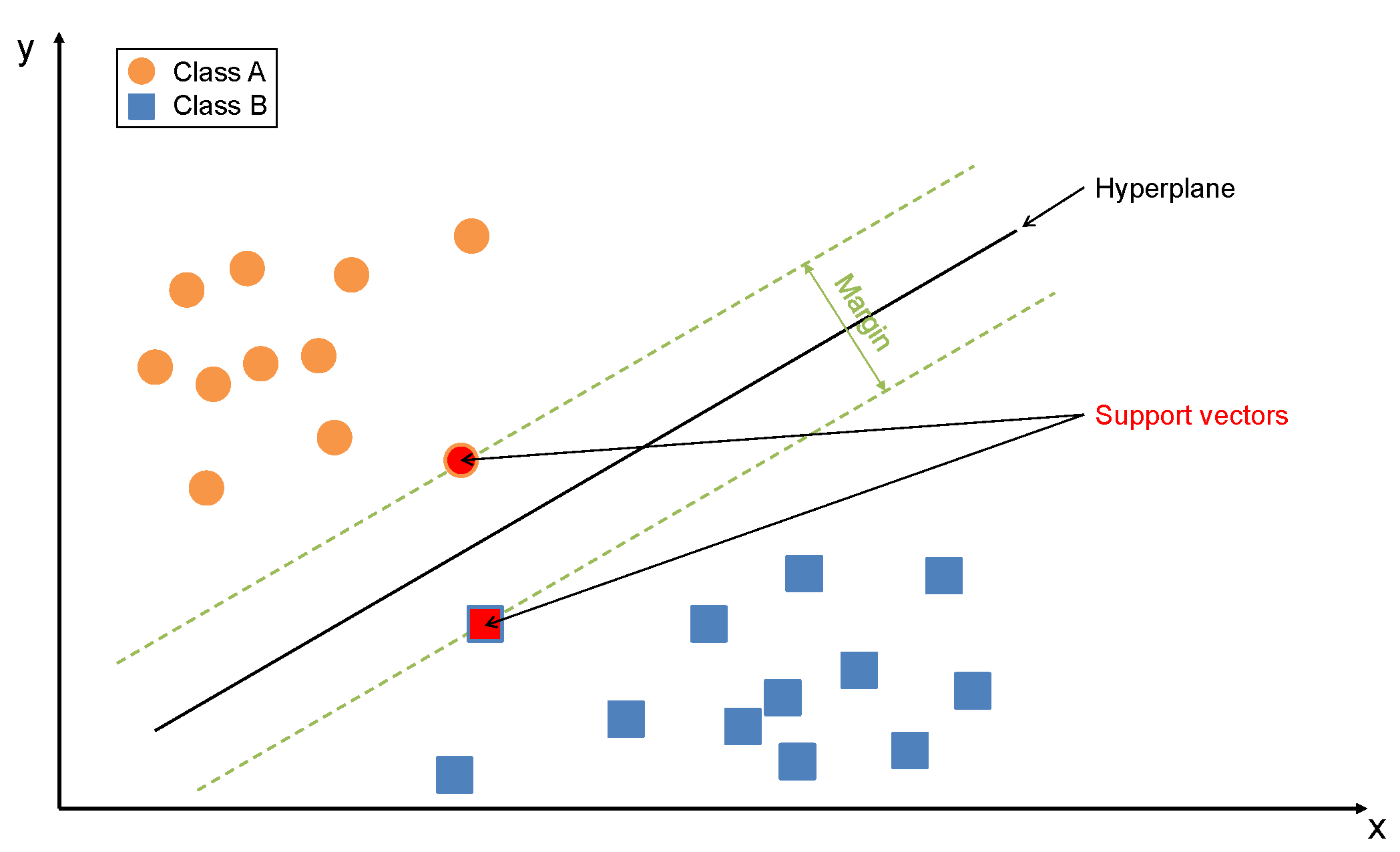
Figure 4.
The architecture of the Random Forest algorithm.
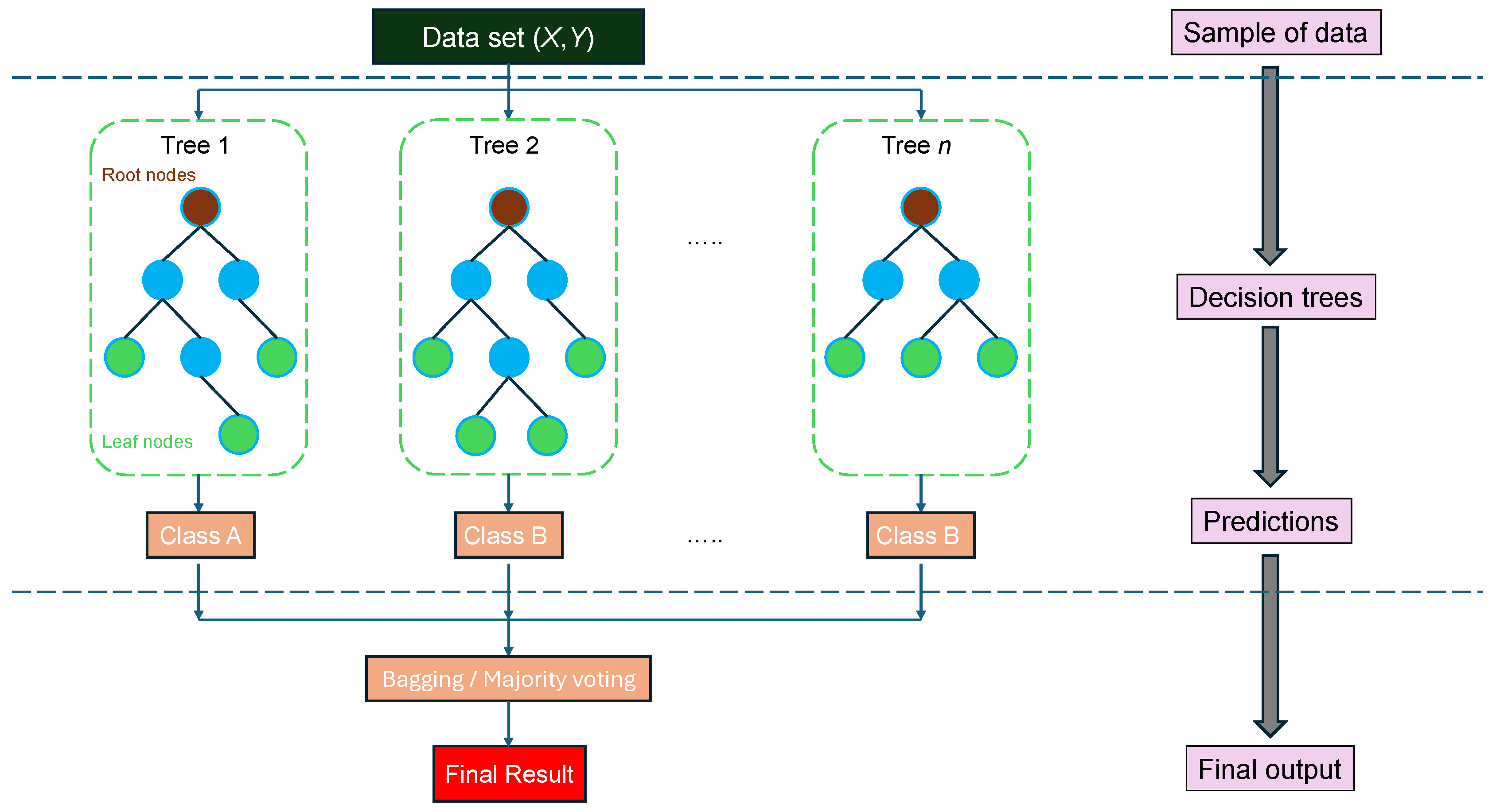
Figure 5.
The architecture of the XGBoost algorithm.
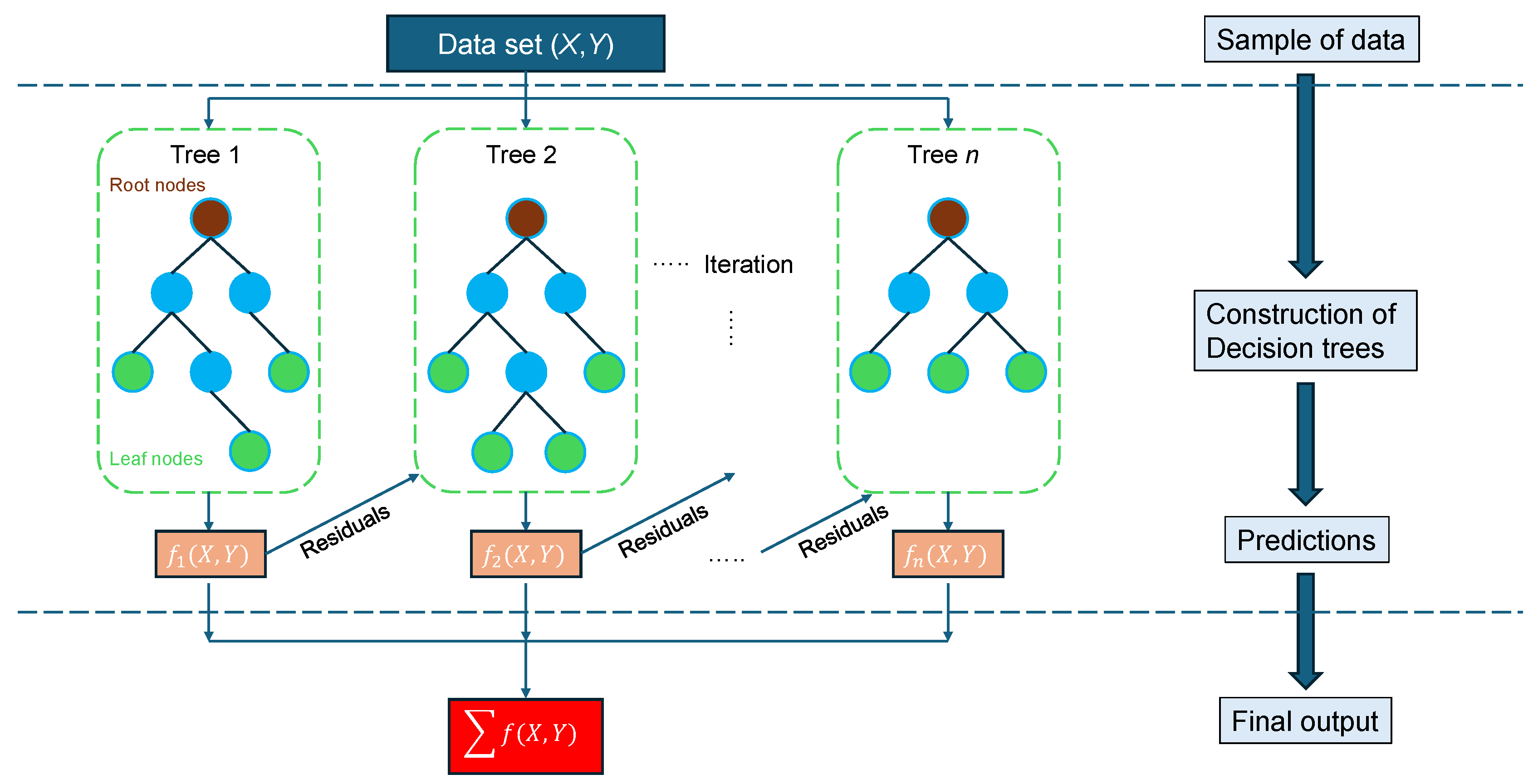
Figure 6.
Geomorphological map of the study area—Peneus river basin—along with its main hydrographic network. Coordinate System: GGRS87/Greek Grid (EPSG:2100).
Figure 6.
Geomorphological map of the study area—Peneus river basin—along with its main hydrographic network. Coordinate System: GGRS87/Greek Grid (EPSG:2100).
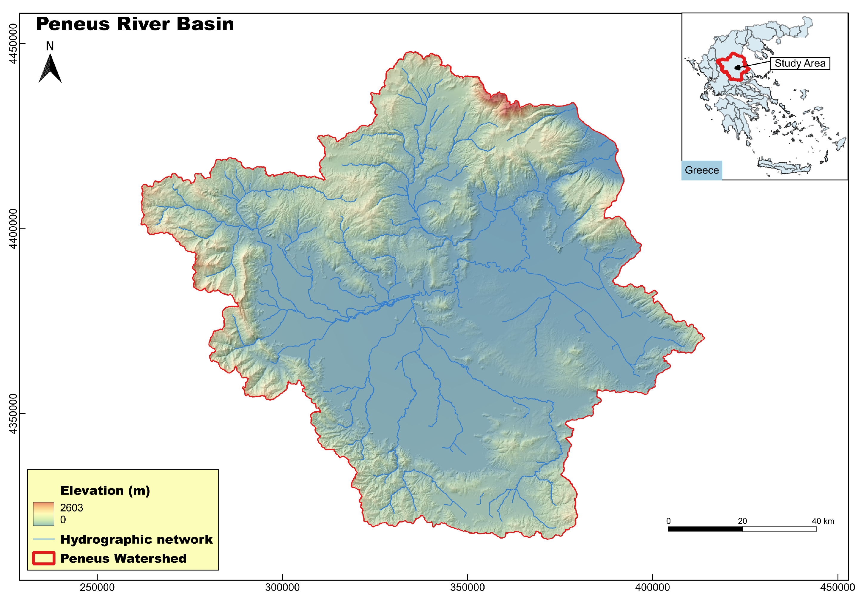
Figure 7.
Satellite image showing the area flooded by Storm Daniel. The left red part indicates no satellite coverage. Source: Sentinel-1. Coordinate System: GGRS87/Greek Grid (EPSG:2100).
Figure 7.
Satellite image showing the area flooded by Storm Daniel. The left red part indicates no satellite coverage. Source: Sentinel-1. Coordinate System: GGRS87/Greek Grid (EPSG:2100).
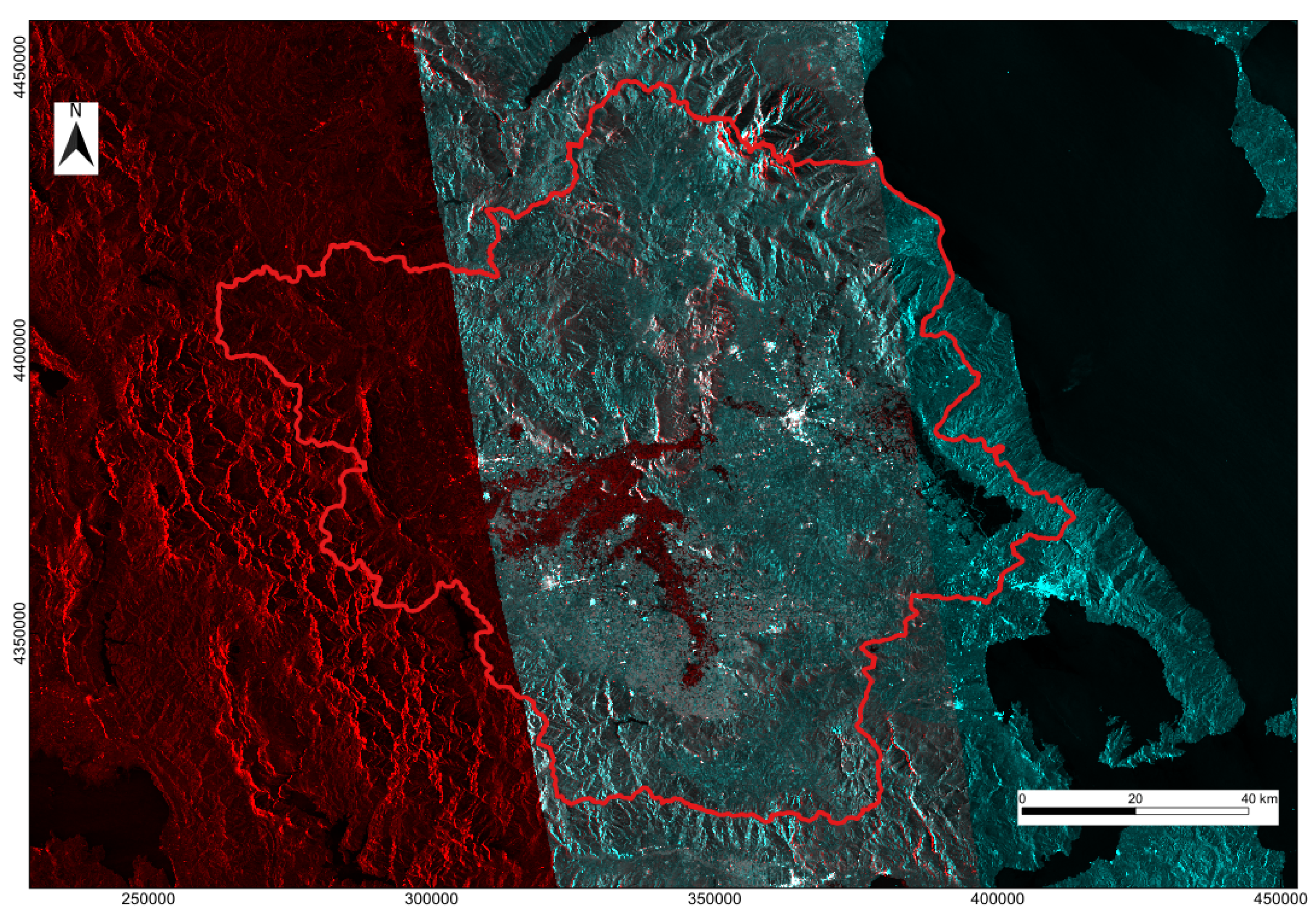
Figure 9.
Pearson correlation matrix of all input (independent) variables.
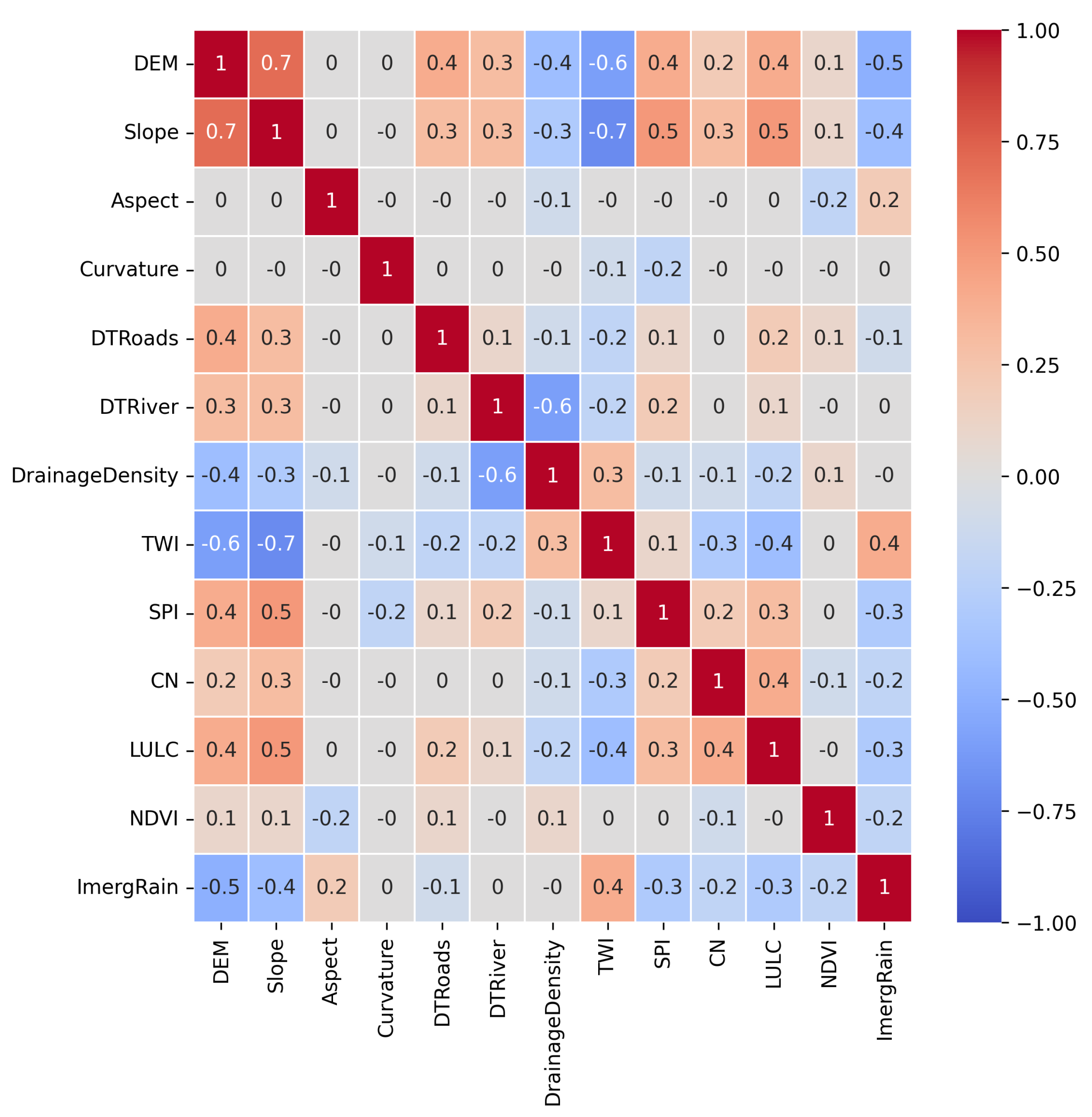
Figure 10.
Confusion matrices showing model performance on the test dataset. (a) LR. (b) SVM. (c) RF. (d) XGBoost.
Figure 10.
Confusion matrices showing model performance on the test dataset. (a) LR. (b) SVM. (c) RF. (d) XGBoost.
| (a) | (b) |
| (c) | (d) |
Figure 11.
Comparison analysis of models performance through ROC curve and AUC score, evaluated on test dataset.
Figure 11.
Comparison analysis of models performance through ROC curve and AUC score, evaluated on test dataset.
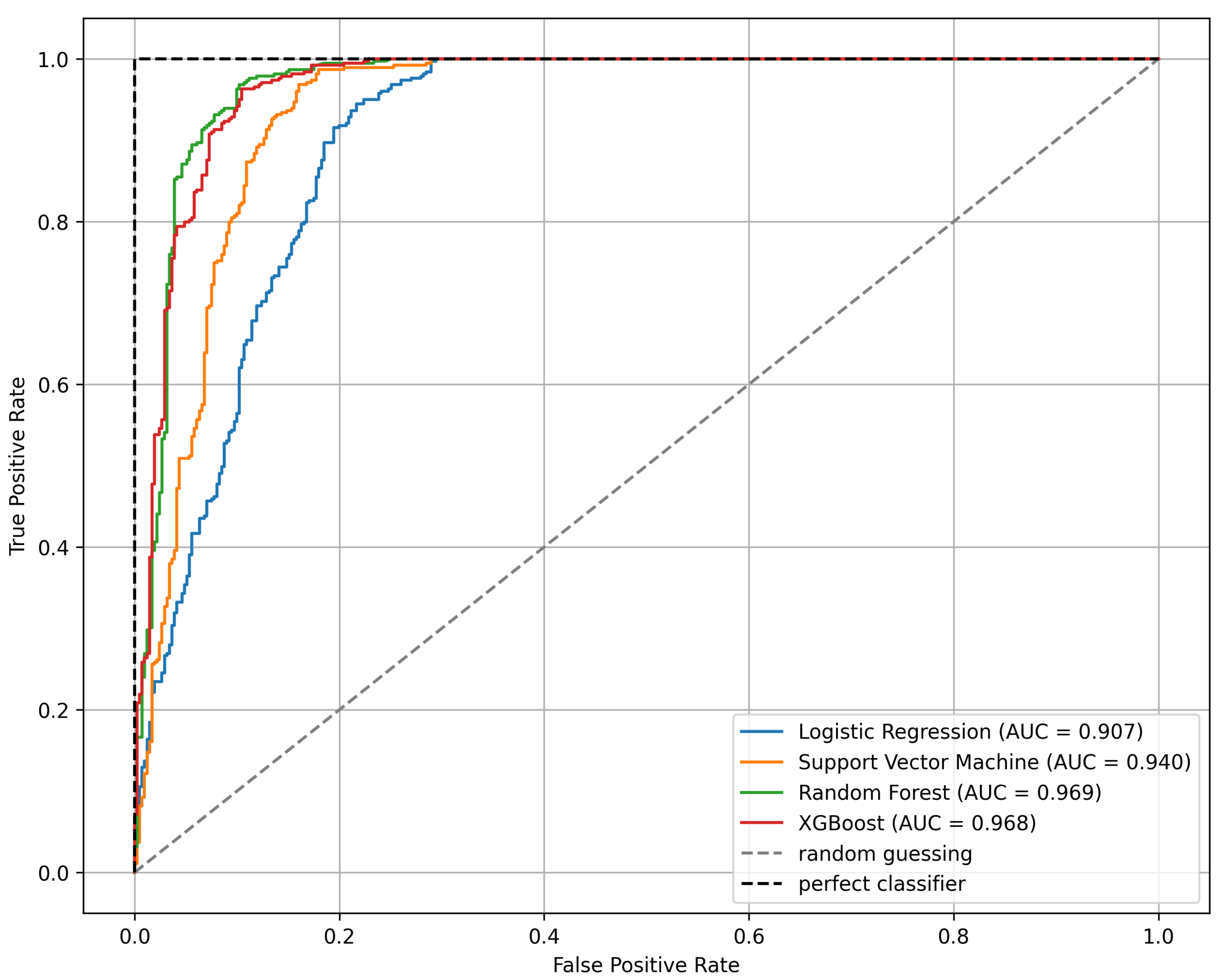
Figure 12.
Flood susceptibility maps of Peneus river basin for each of the trained models. (a) LR. (b) SVM. (c) RF. (d) XGBoost.
Figure 12.
Flood susceptibility maps of Peneus river basin for each of the trained models. (a) LR. (b) SVM. (c) RF. (d) XGBoost.
| (a) | (b) |
| (c) | (d) |
Figure 13.
Feature importance’s for the RF model across different methods. (a) Mean Decrease Impurity. (b) Permutation-based.
Figure 13.
Feature importance’s for the RF model across different methods. (a) Mean Decrease Impurity. (b) Permutation-based.
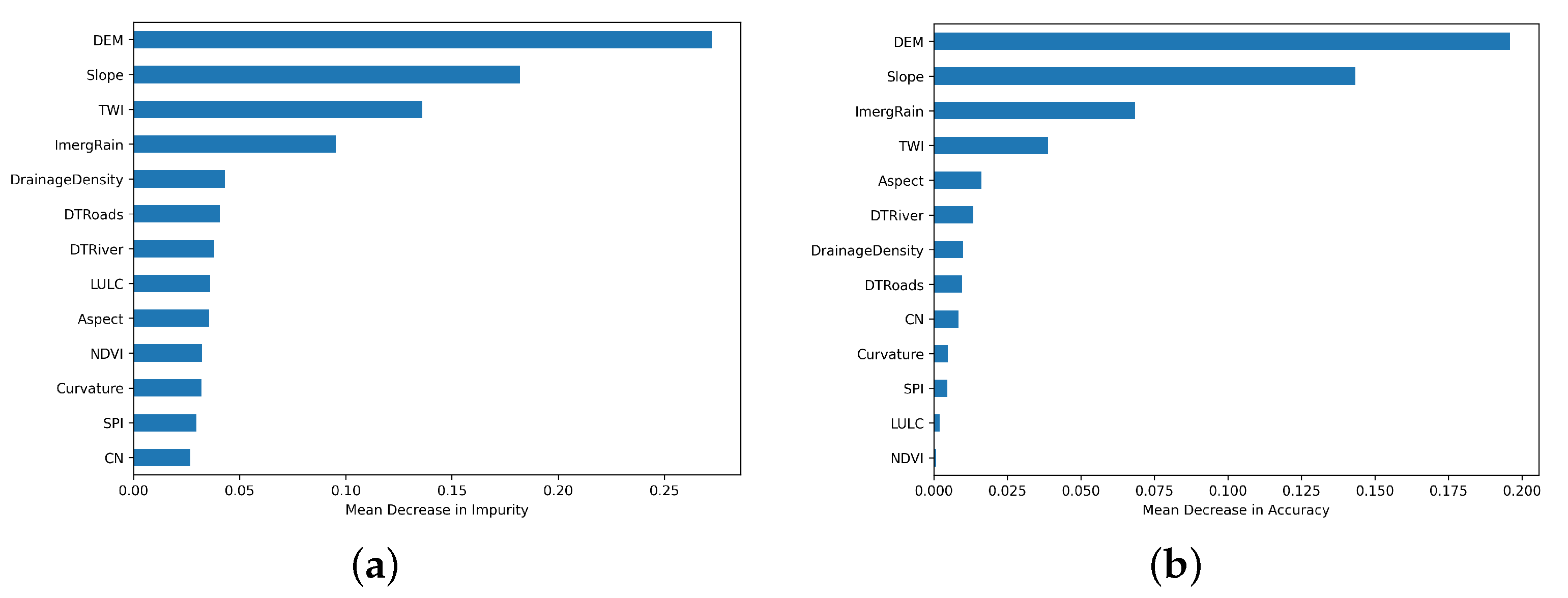
Figure 14.
Flood susceptibility maps of Peneus river basin with Random Forest for different initial training data. (a) Train with left-half catchment. (b) Train with right-half catchment.
Figure 14.
Flood susceptibility maps of Peneus river basin with Random Forest for different initial training data. (a) Train with left-half catchment. (b) Train with right-half catchment.
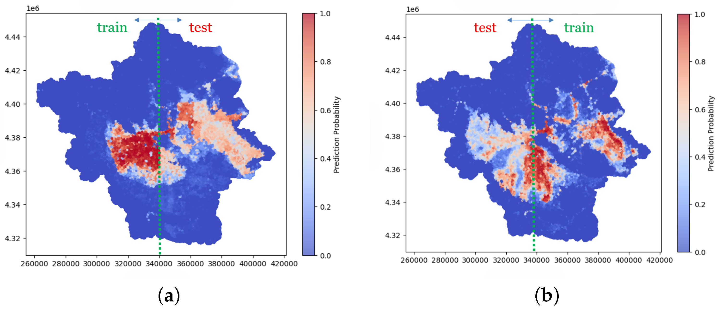
| (a) | (b) |
Figure 15.
Comparison analysis of Random Forest models trained in different initial training data, through ROC and AUPRC curve (Train All: trained using data from the entire basin, Train Left: trained using data from the left side of the basin, Train Right: trained using data from the right side of the basin). (a) ROC curves. (b) AUPRC curves.
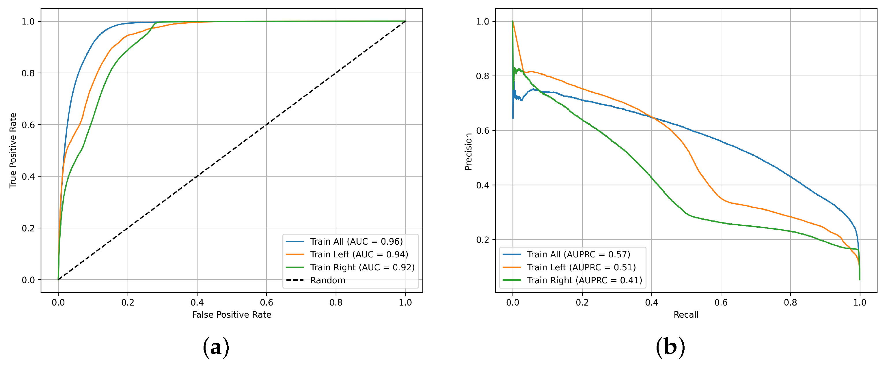
| (a) | (b) |
Figure 16.
Rainfall for years and h.
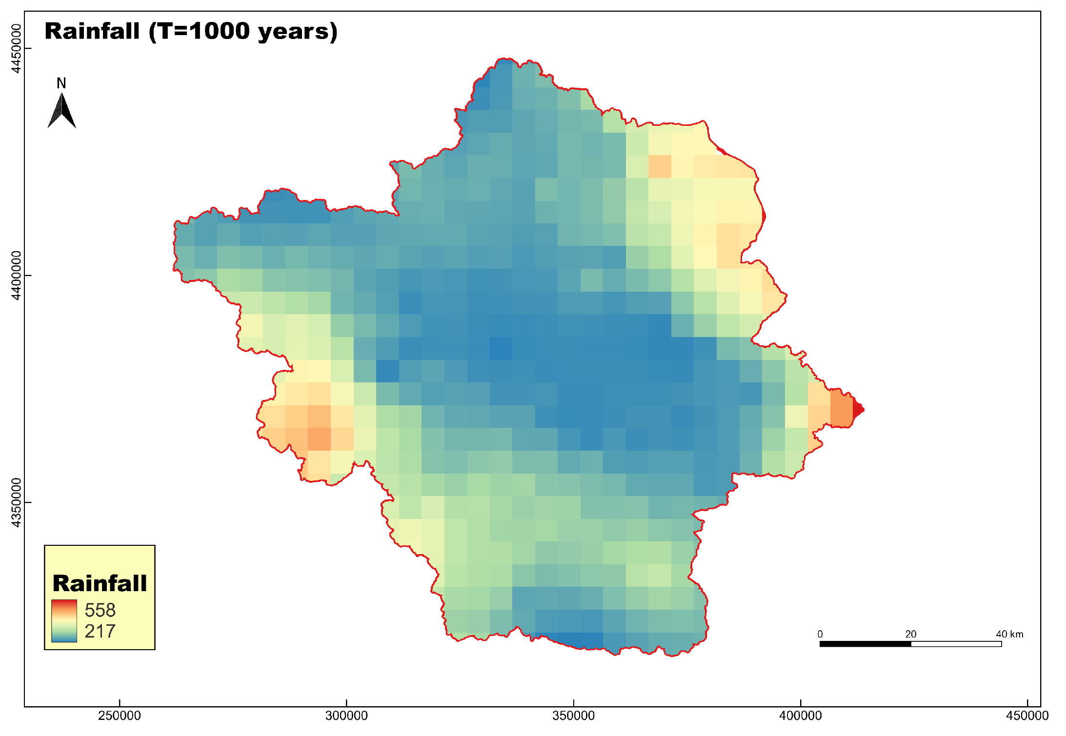
Figure 17.
FSM for Peneus basin based on a rainfall scenario for years and h.
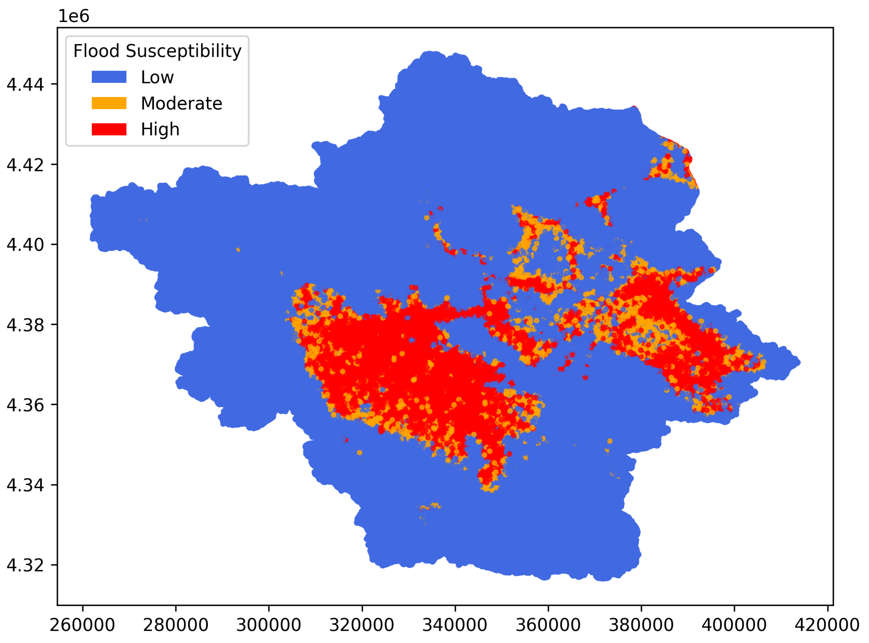
Table 4.
Values derived from hyperparameter optimization task for the Logistic Regression (LR), Support Vector Machine (SVM), Random Forest (RF), eXtreme Gradient Boosting (XGBoost).
Table 4.
Values derived from hyperparameter optimization task for the Logistic Regression (LR), Support Vector Machine (SVM), Random Forest (RF), eXtreme Gradient Boosting (XGBoost).
| Model | Hyperparameter values |
|---|---|
| LR | max iter=1000, scoring=’accuracy’, multi class=’auto’, solver=’lbfgs’ |
| SVM | C=2, gamma=’scale’, kernel=’radial basis function (rbf)’, scaler=’StandardScaler’ |
| RF | no. estimators=200, max depth=20, min samples split=2, min samples leaf=1, max features=’sqrt’ |
| XGBoost | no. estimators=100, max depth=7, learning rate=0.1, subsample=1.0, colsample by tree=0.8 |
Table 5.
Models results for each evaluation metric on the test set. The best performing model for each metric is highlighted in bold.
Table 5.
Models results for each evaluation metric on the test set. The best performing model for each metric is highlighted in bold.
| Model | Accuracy | Precision | Recall / Sensitivity | Specificity | F1 score |
|---|---|---|---|---|---|
| LR | 0.85 | 0.76 | 1.00 | 0.71 | 0.86 |
| SVM | 0.86 | 0.78 | 0.99 | 0.75 | 0.88 |
| RF | 0.93 | 0.89 | 0.97 | 0.89 | 0.93 |
| XGBoost | 0.93 | 0.89 | 0.96 | 0.90 | 0.93 |
Disclaimer/Publisher’s Note: The statements, opinions and data contained in all publications are solely those of the individual author(s) and contributor(s) and not of MDPI and/or the editor(s). MDPI and/or the editor(s) disclaim responsibility for any injury to people or property resulting from any ideas, methods, instructions or products referred to in the content. |
© 2025 by the authors. Licensee MDPI, Basel, Switzerland. This article is an open access article distributed under the terms and conditions of the Creative Commons Attribution (CC BY) license (http://creativecommons.org/licenses/by/4.0/).
Copyright: This open access article is published under a Creative Commons CC BY 4.0 license, which permit the free download, distribution, and reuse, provided that the author and preprint are cited in any reuse.


