
Submitted:
05 March 2025
Posted:
06 March 2025
You are already at the latest version
Abstract
The frequency and intensity of extreme precipitation and temperature events has been increasing over the past decades. These changes could impact daily exposure to high concentrations of pollutants like SO2, NO2, Ozone and particulate matter (PMx), exacerbating risks for numerous health problems. We used monitor based measurements of daily concentrations of seven common pollutants and raster based climate datasets to test associations of precipitation and temperature with daily pollutant levels for the years 2005 to 2022. Concentrations and climate change data were mapped using latitude longitude locations of pollution monitors. We visualized daily measures of pollutants and temperature to explore possible same-day correlation between each. To explore lag associations of pollutants and climate variables, we used cross correlation functions and identified lag days where the association was strongest. We found that Ozone and PM10 had strong positive correlations with temperature (Pearson corr: .31 and .25 respectively), while NO2 had strong negative correlations (Pearson corr: -.21). Precipitation was negatively associated with nearly all pollutants. Cross-correlations suggested that there were important lag associations of temperature and precipitation pollutants, but that specific predictive lag days varied by pollutant. Further study of pollutant concentration patterns would allow researchers to better predict airborne pollutant exposures based on available daily weather data, thus better assessing potential risks to human health for at risk populations.
Keywords:
air pollution
; climate change
; extreme weather
; heat
; precipitation
1. Introduction
The intensity, frequency and duration of extreme weather events including heatwaves and catastrophic precipitation events has been increasing across the world [1,2]. Ambient air pollutants such as particulate matter (PM), carbon monoxide (CO), ozone (O3) and sulfur dioxide (SO2) all have demonstrated impacts on human mental and physical health [3,4,5] and contribute significantly to global mortality, particularly from respiratory causes [6,7,8]. Some research has suggested that the combination of concentrations of various air pollutants and temperature and precipitation might have synergistic effects on health [9]. Understanding patterns of association of climate variables such as temperature and precipitation with concentrations of important air pollutants would help to better characterize short and long term changes in specific health risks.
Previous research demonstrates that elevated levels of ozone concentration due to temperature changes might results in increases in worldwide mortality from a number of causes [10]. High concentrations of and might increase incidence of death and increase health expenditures [11,12] and the inhalation of associated microplastics might also have important implications for health [13]. might have implications for urban health as it is a precurser gs to the formation of Ozone and common in auto emissions [14]. Air pollution exposures might rise with changes in patterns of temperature and precipitation by influencing the photo-chemical production of secondary pollutants and increasing particulate emissions [15].
Our research examines temporal associations of concentrations of common pollutants with patterns of temperature and precipitation to provide information to support efforts to predict health outcomes. We want to examine how temperature change and precipitation would lead to changes in temporal patterns of specific air pollutants. We also seek to discover whether there are lag associations of climate variables that might be used to predict sudden or intense changes in airborne concentrations of various air pollutants.
This research explores associations of climate variables with seven common air pollutants using raster-based data for temperature and precipitation and monitor-based air pollution measurements. We will not only describe same-day associations of temperature and precipitation and air pollutant concentrations, but will also explore lag associations. We will explore how not only daily changes in climate impact air pollutant concentrations but will also explore how short-term past changes in precipitation are associated with concentrations of specific air pollutants today. This research will add to a growing literature on climate and air pollution and hope that the results of our work will extend to explorations of health risks.
1.1. Hypotheses to be tested
This research will test two main hypotheses:
- Hypothesis 1: Temporal patterns of temperature and precipitation will be correlated with temporal patterns of specific air pollutants. We suspect that the patterns of association of temperature and precipitation will differ both in magnitude and direction by air pollutant.
- Hypothesis 2: There will be lag patterns of associations of temperature/precipitation with specific ambient air pollutants. The impacts of temperature/precipitation on air pollutant concentrations will not be felt instantaneously, but rather will arise days or weeks after temp/precip changes.
2. Methods
2.1. Data
This research uses freely available daily air pollutant monitor data from Environmental Protection Agency of the United States [16]. This system comprises more than 4,000 outdoor monitoring stations located throughout the United States and its territories. Each monitor measures concentrations of up to six or more pollutants on a daily basis. Data are collected from each monitoring station and added the Air Quality System database [16], which is made available for free to the public. This research focuses on six classes of air pollutants: Ozone (), Particulate matter ( and ), Carbon monoxide (CO), Nitrogen dioxide (), Sulfur dioxide (), and lead (Pb). These six common air pollutants each present unique health risks documented in numerous research studies.
Researchers downloaded daily data for each site, retaining the monitor identification number (ID) and county for the all available observations between January, 2005 and February, 2022. Target states included the Midwestern "Great Lakes" States of Illinois, Indiana, Michigan, Ohio, Pennsylvania and Wisconsin, which are all demographically and developmentally similar states in temperate region of the United States.
Daily maximum temperatures and precipitation (rain+melted snow) for every county in each of the target states were extracted from raster-based data sets obtained from the PRISM Climate Group at Oregon State University [17]. We merged temperature and precipitation based on the county location of air pollution monitors. Though we recognize that both precipitation and temperature can be highly localized, it might also be highly variable at that location, due to a number of factors. As one of the goals of this research is to identify possible contributions of average temperature and precipitation over a wide space in order to support possible efforts to predict changes in ambient pollutant concentrations, it was decided that county level averages would be sufficient.
2.2. Statistical Methods
We visualize all six pollution measures, temperature and precipitation by plotting the series of daily means to evaluate any possible seasonality and trend. Next, we calculated Pearson’s correlation coefficients of daily data for all pollutants with temperature and precipitation at every location. We then calculate cross-correlations of all pollutants with temperature and precipitation to explore same day and lag associations of pollution with climate variables. The sample cross correlation function (CCF) can help identify lags of the one variable that might a useful predictor of another. Cross correlations can be expressed in lags of x before or after observation y. This can help us assess how changes in one variable are associated with changes in another, both for x with y and for y with x. That is, we can explore which variable leads another and which variable might follow. The method allows us to shift the position of each series relative to one another by k time units and calculating a correlation coeffcient between the two series for each unit shift k. We can then compare the series for a range of time differences and determine the time lag where the correlation between the two series is strongest. For this research, we use the ccf() function in R. This function uses the standard deviations and the stationary mean of the two series to calculate the correlation allowing for temporal autocorrelation within time series. We visualize the cross-correlations. We then numerically find the lag at which correlations between pollutants and temperature/precipitation are strongest.
3. Results
After compiling all pollutant data recorded between January 1, 2005 and February 1, 2022, we found missing daily observations in several of the monitor sites. Some sites contain only observations for short periods of time, presumably due to time of initial construction of the monitor or device failure. Ozone and PM2.5 have the most monitor sites. For PM10, SO2, CO, and NO2, there were few monitors until the year 2016. For Pb, there are few monitors across the time frame, and many monitors worked only for a short period of time. For this research, we only used monitor data with relatively complete (>95% non-missing) data within the target time window.
We visualized the time series of each pollutant, temperature and precipitation. We observed strong seasonal patterns of Ozone, CO and . We confirmed seasonality by time series decomposition (not shown). Variability of NO2, PM2.5, PM10 and SO2 decreased over time. Concentrations of CO have increased since 2015. See Figure 1 for daily time plots for each of the other the pollutants. Ozone and CO concentrations did not decrease over time. However, has decreased since 2011. We observed the decreasing trend of since 2005, resulting from regulations of . reaches its maximum in 2017, but has decreased since then. Years 2005-2008 displayed increasing , but has decreased and reached a constant value since 2015. Though we did not find a significant trend in Pb concentration, we can see that Pb concentrations are very high in the year 201 but decreases then. See Figure 2 for full results.
We visualized the two climate variables and observed seasonal patterns in daily maximum temperatures across all counties in target states. We also observed seasonal patterns in daily precipitation, noting maximum precipitation changes over time and which counties have increased chance of extreme precipitation events.
Table 1 shows the mean daily concentrations for each of the seven pollutants we examined. While each measure the concentrations of pollutants, the scale of each pollutant is different. We standardized each pollutant to allow comparisons across all of the. we found a negative association between temporal patterns of precipitation and temporal patterns of specific air pollutant concentrations such as , , , , Ozone. There was no observable association with CO and Pb. Temperature was positively associated with temporal patterns of Ozone and concentration. No observable association with Pb, , , and CO was found.
We used pre-whitening strategies to assess the climate data and examine the lag response of the pollutant concentration. We found that maximum temperature is positively associated with CO concentration after 1 and 3 days. Maximum temperature is positively associated with concentration after 3 and 7 days, and negatively associated with concentration after 6 days. Maximum temperature is positively associated with concentration after 3,5,13,16 days, and negatively associated with concentration after 4 and 12 days. Maximum temperature is positively associated with concentration 1 day and 2 days afterward. Maximum temperature is positively associated with concentration after 1 and 5 days, and negatively associated with concentration after 4 days. Maximum temperature is positively associated with Pb concentration after 5 days, and negatively associated with Pb concentration after 4 and 6 days. Maximum temperature is positively associated with Ozone concentration after 1 and 2 days.
We found that precipitation is positively associated with CO concentration after 8 days. We found no significant association between lag response of concentration and precipitation. Precipitation is negatively associated with concentration after 1 day. Precipitation is positively associated with concentration after 4 days. Precipitation is negatively associated with concentration after 8 days. Precipitation is negatively associated with Pb concentration after 5 days and positively associated with Pb concentration after 6 days. Precipitation is positively associated with Ozone concentration 4-10 days afterward.
Figure 3.
Cross correlations of pollutants with precipitation
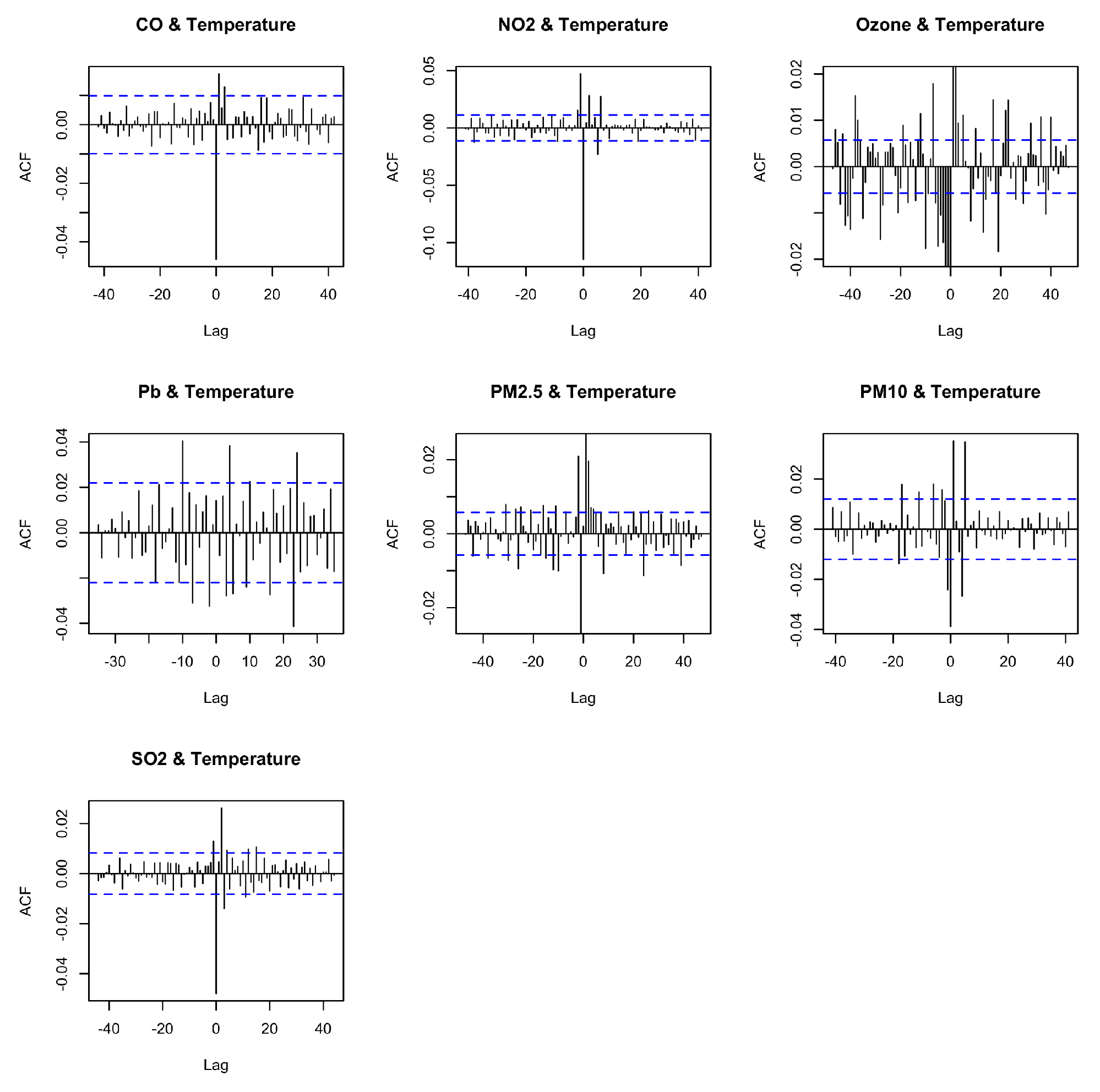

Table 2.
Significant lag associations between pollutants and climate variables.
| Pollutants | Lag temp | Lag precip |
|---|---|---|
| CO | 3 | 8 |
| 7 | NA | |
| Ozone | 2 | 10 |
| Pb | 5 | 6 |
| 2 | 4 | |
| 4 | 8 | |
| 12 | 1 |
4. Discussion
We found a moderately strong positive correlations between PM10, Ozone and daily maximum temperature, suggesting that over all increases in temperatures or sudden extreme heat events might lead to rapid increases in exposure to these pollutants. As PM10 and Ozone both have bean associated with serious physical and mental health risks [18,19], changes in climate might exacerbate incidence for health conditions association with these pollutants.
Nearly all pollutants showed lag associations with daily max temperature and precipitation, but the association varied by pollutants. In the future, we may use these associations and detection of extreme climate events to predict the level of air pollutants, incorporating the level of air pollutants into weather forecast. The precise prediction of changing patterns of pollutants can be useful for those who need to avoid absorbing certain air pollutants. For example, people with heart or lung diseases are acute to short-term and long-term exposure to PM2.5. Infants, children and older adults should limit their exposure to PM2.5. A thorough understanding of associations between pollutants and climate variables would allow for better public health outcomes.
The limited spatial distribution of air quality impacts the ability to test associations of climate and pollutant concentrations across a varied set of contexts. Most air quality monitors were located in or around urban centers. While concentrations of air pollutants are generally lower and air quality better in rural areas of the United States compared to urban areas [20], there might be strong variation by context, the nature of local agricultural activities [21,22] and by level of urbanicity [23,24]. The lack of pollutant monitors in rural areas complicates making comparisons between rural and urban exposures, biases results to developed cities, and obscures rural-specific air pollution risks [25].
If daily maximum temperature and precipitation are important causal predictors of concentrations of some pollutants, climate data can be easily leveraged to create early warning systems or help inform public health professionals where to allocated resources to prevent air quality related health problems. Through modelling and the breadth of data available, we can design systems to protect the public health. Future efforts might also explore differences in patterns of climate and air pollution in different geographic and demographic areas of the United States.
Author Contributions
Conceptualization, X.L. and P.S.L.; methodology, X.L. and P.S.L.; software,X.L. and J.J.; validation, X.L.; formal analysis, X.L. and P.S.L.; investigation, X.L. and P.S.L.; resources, P.S.L.; data curation, X.L. and J.J.; writing—original draft preparation, X.L., P.S.L.,A.N.; writing—review and editing, X.L., P.S.L.,A.N.; visualization, X.L.; supervision, P.S.L.; project administration, P.S.L; funding acquisition, P.S.L. All authors have read and agreed to the published version of the manuscript.
Funding
This project was funded through a grant from the University of Michigan Institute for Global Change Biology (IGCB).
Institutional Review Board Statement
Not applicable
Informed Consent Statement
Not applicable
Data Availability Statement
All code is available at:
Acknowledgments
We thank the University of Michigan’s Undergraduate Research Opportunity Program (UROP) for supporting this work.
Conflicts of Interest
The authors declare no conflicts of interest.
References
- Perkins, S.E.; Alexander, L.V.; Nairn, J.R. Increasing frequency, intensity and duration of observed global heatwaves andwarmspells. Geophysical ResearchLetters 2012, 39. [Google Scholar] [CrossRef]
- Perkins-Kirkpatrick, S.E.; Lewis, S.C. Increasingtrend sin regional heatwaves. Nature Communications 2020, 11. [Google Scholar] [CrossRef]
- Liu, C.; Chen, R.; Sera, F.; Vicedo-Cabrera, A.M.; Guo, Y.; Tong, S.; Coelho, M.S.; Saldiva, P.H.; Lavigne, E.; Matus, P.; et al. AmbientParticulateAirPollutionandDailyMortalityin652Cities. New England Journal of Medicine 2019, 381, 705–715. [Google Scholar] [CrossRef] [PubMed]
- Zhang, B.; Weuve, J.; Langa, K.M.; D’Souza, J.; Szpiro, A.; Faul, J.; Mendesde Leon, C.; Gao, J.; Kaufman, J.D.; Sheppard, L.; et al. ComparisonofParticulateAirPollutionFromDifferentEmissionSourcesandIncident Dementia in the US. JAMA Internal Medicine 2023, 183, 1080. [Google Scholar] [CrossRef]
- Berman, J.D.; Burkhardt, J.; Bayham, J.; Carter, E.; Wilson, A. Acute Air Pollution Exposure and the Risk of Violent Behavior in the UnitedStates. Epidemiology 2019, 30, 799–806. [Google Scholar] [CrossRef]
- Hu, Z. Spatial analysis of MODISaerosoloptical depth, PM2.5, and chronic coronary heart disease. Int. J. Health Geogr. 2009, 8, 27. [Google Scholar]
- Dominski, F.H.; LorenzettiBranco, J.H.; Buonanno, G.; Stabile, L.; GameirodaSilva, M.; Andrade, A. Effects of airpollutiononhealth:Amappingreviewofsystematicreviewsandmeta-analyses. Environmental Research 2021, 201, 111487. [Google Scholar] [CrossRef]
- Lelieveld, J.; Evans, J.S.; Fnais, M.; Giannadaki, D.; Pozzer, A. The contribution of outdoor air pollution sources to premature mortality on a global scale. Nature 2015, 525, 367–371. [Google Scholar] [PubMed]
- Anenberg, S.C.; Haines, S.; Wang, E.; Nassikas, N.; Kinney, P.L. Synergistichealtheffectsofairpollution, temperature, andpollenexposure:asystematicreviewofepidemiologicalevidence. EnvironmentalHealth 2020, 19. [Google Scholar] [CrossRef]
- Lou, J.; Wu, Y.; Liu, P.; Kota, S.H.; Huang, L. Healtheffectsofclimatechangethroughtemperatureandair pollution. Curr.Pollut.Rep. 2019, 5, 144–158. [Google Scholar]
- Dai, J.; Chen, R.; Meng, X.; Yang, C.; Zhao, Z.; Kan, H. Ambientairpollution, temperatureandout-of-hospital coronarydeathsinShanghai, China. Environ.Pollut. 2015, 203, 116–121. [Google Scholar] [PubMed]
- Hou, Q.; An, X.; Tao, Y.; Sun, Z. Assessmentofresident’sexposurelevelandhealtheconomiccostsofPM10 in Beijingfrom2008to2012. Sci. TotalEnviron. 2016, 563-564, 557–565. [Google Scholar]
- Roy, D.; Kim, J.; Lee, M.; Kim, S.; Park, J. PM10-boundmicroplasticsandtracemetals:Apublichealth insight fromtheKoreansubwayandindoorenvironments. Journal ofHazardousMaterials 2024, 477, 135156. [Google Scholar] [CrossRef]
- Costa, S.; Ferreira, J.; Silveira, C.; Costa, C.; Lopes, D.; Relvas, H.; Borrego, C.; Roebeling, P.; Miranda, A.I.; Teixeira, J.P. Integratinghealthonairqualityassessment–reviewreportonhealthrisksoftwomajor EuropeanoutdoorairpollutantsPMandNO2. J. Toxicol.Environ.HealthBCrit.Rev. 2014, 17, 307–340. [Google Scholar]
- Anenberg, S.C.; Haines, S.; Wang, E.; Nassikas, N.; Kinney, P.L. Synergistichealtheffectsofairpollution, temperature, and pollenexposure:asystematicreviewofepidemiologicalevidence. Environ.Health 2020, 19, 130. [Google Scholar]
- Environmental Protection Agency. Air Data Basic information. website 2023. [Google Scholar]
- Northwest Alliance for Computational Scienceand Engineering. PRISM Climate Data. website.
- Manisalidis, I.; Stavropoulou, E.; Stavropoulos, A.; Bezirtzoglou, E. Environmental and Health Impact sof Air Pollution: A Review. FrontiersinPublicHealth 2020, 8. [Google Scholar] [CrossRef]
- Zhao, T.; Markevych, I.; Romanos, M.; Nowak, D.; Heinrich, J. Ambientozoneexposureandmental health: Asystematicreviewofepidemiologicalstudies. EnvironmentalResearch 2018, 165, 459–472. [Google Scholar]
- Strosnider, H.; Kennedy, C.; Monti, M.; Yip, F. RuralandUrbanDifferencesinAirQuality, 2008–2012, and Community DrinkingWaterQuality, 2010–2015—UnitedStates. MMWR. SurveillanceSummaries 2017, 66, 1–10. [Google Scholar] [CrossRef]
- Hendryx, M.; Fedorko, E.; Halverson, J. PollutionSourcesandMortalityRatesAcrossRural-UrbanAreas in theUnitedStates:PollutionSourcesandMortalityRates. The JournalofRuralHealth 2010, 26, 383–391. [Google Scholar] [CrossRef]
- Kilpatrick, D.J.; Hung, P.; Crouch, E.; Self, S.; Cothran, J.; Porter, D.E.; Eberth, J.M. GeographicVariationsin Urban-Rural ParticulateMatter(PM2.5)ConcentrationsintheUnitedStates, 2010–2019. GeoHealth 2024, 8. [Google Scholar] [CrossRef]
- Liang, L.; Gong, P. Urbanandairpollution:amulti-citystudyoflong-termeffectsofurbanlandscape patterns onairqualitytrends. Scientific Reports 2020, 10. [Google Scholar] [CrossRef]
- Larson, P.S.; Eisenberg, J.N.S.; Berrocal, V.J.; Mathanga, D.P.; Wilson, M.L. Anurban-to-ruralcontinuum of malaria risk: new analytic approaches characterize pattern sin Malawi. Malaria Journal 2021, 20, //doi.org/10.1186/s12936-021-03950–5. [Google Scholar]
- Wang, Y.; Puthussery, J.V.; Yu, H.; Liu, Y.; Salana, S.; Verma, V. Source sof cellular oxidative potential of water-solublefineambientparticulatematterintheMidwesternUnitedStates. Journal ofHazardousMaterials 2022, 425, 127777. [Google Scholar] [CrossRef]
Figure 1.
Mean concentration of pollutants and associated precipitation and max temperature from 2005-01-01 to 2022-02-01. First row: CO, , Ozone. Second row: Pb, , . Third row: , Max temperature, Precipitation.
Figure 1.
Mean concentration of pollutants and associated precipitation and max temperature from 2005-01-01 to 2022-02-01. First row: CO, , Ozone. Second row: Pb, , . Third row: , Max temperature, Precipitation.
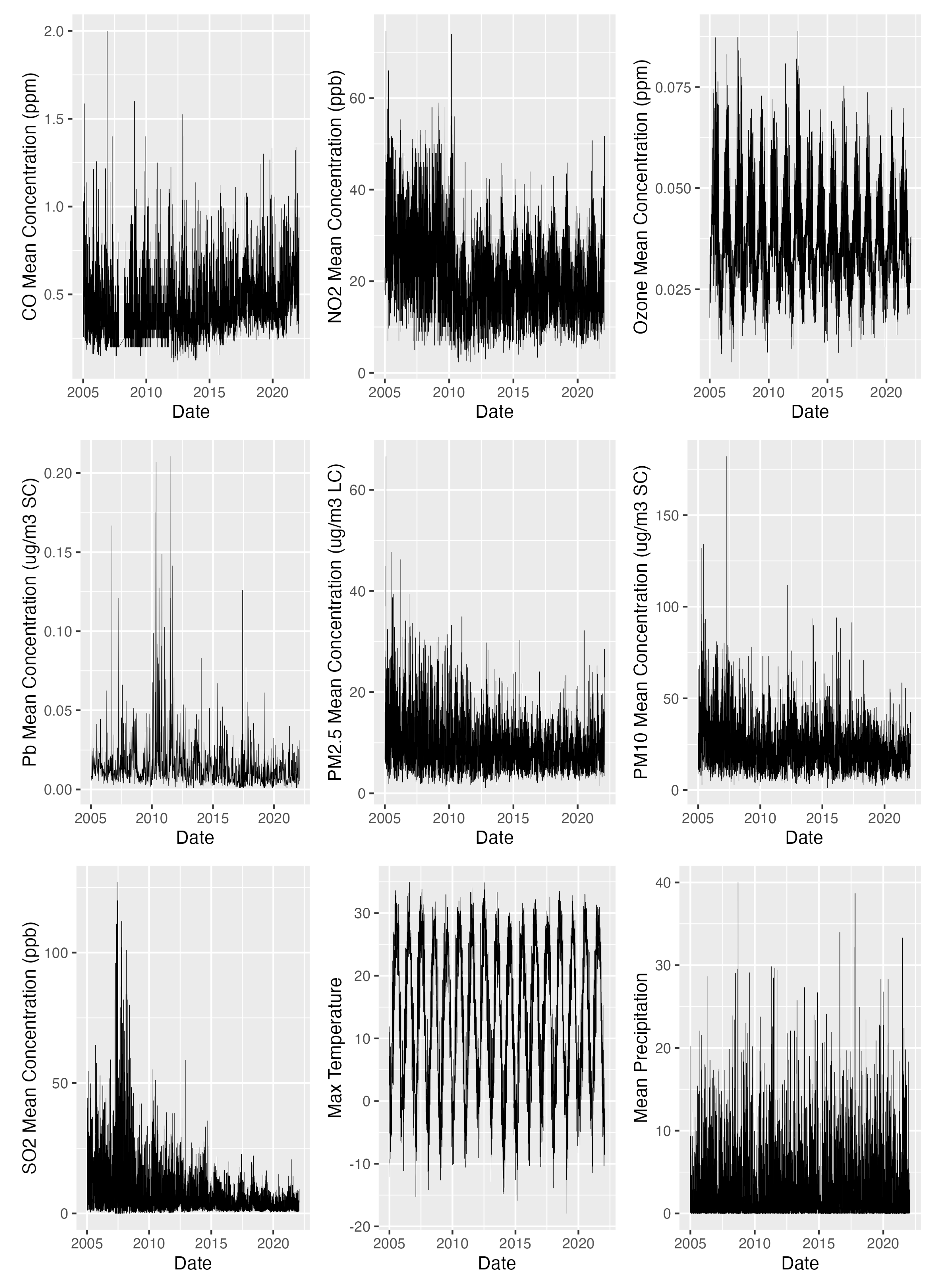
Figure 2.
Cross correlations of pollutants with temperature
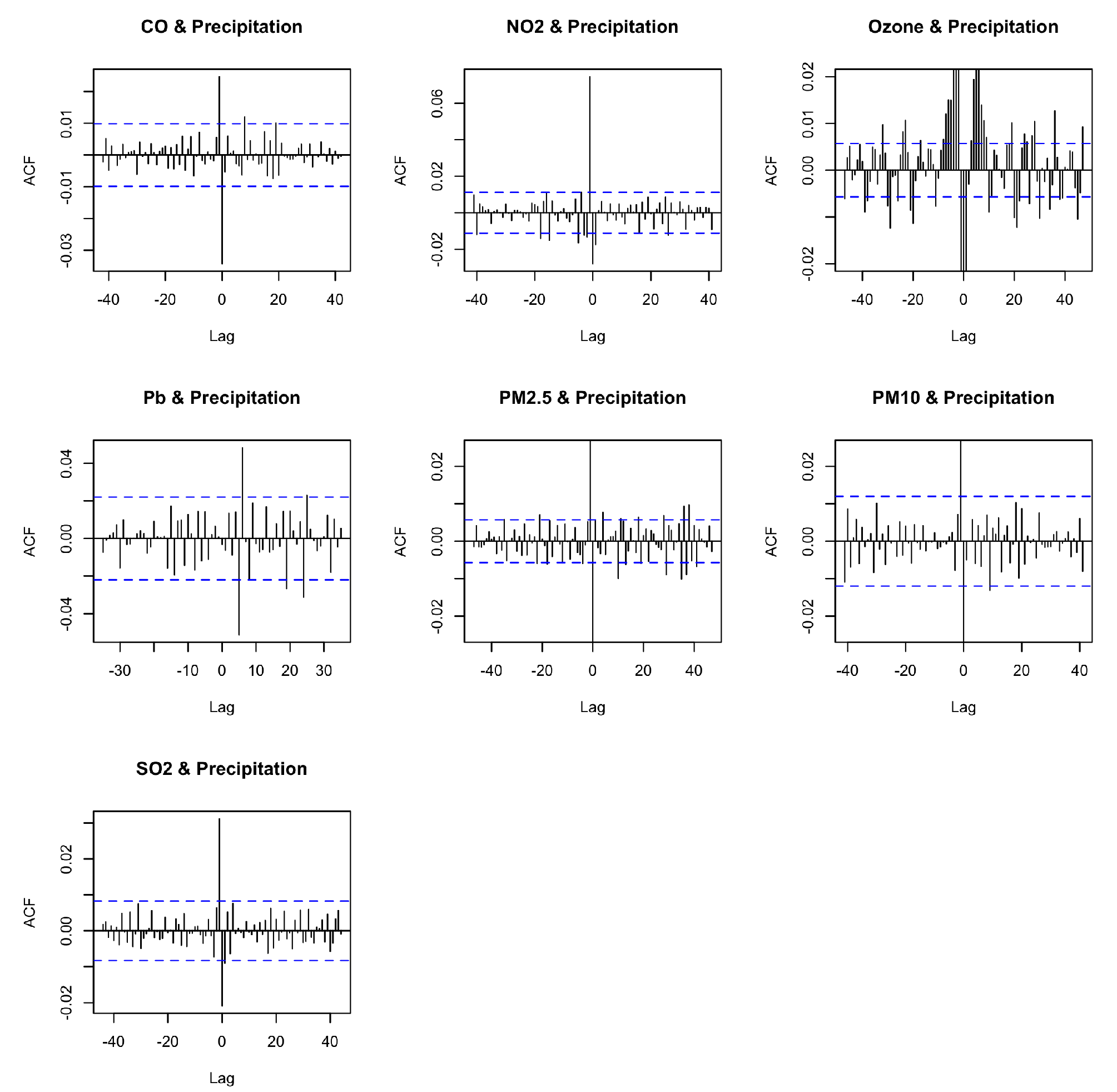
Table 1.
Pollutant’s correlation with climate variables
| Pollutants | Pollutant mean (sd) | Correlation Temp mean (sd) | Correlation Precip mean (sd) |
|---|---|---|---|
| CO | 0.44 (0.25) | -0.02 (0.07) | -0.08 (0.05) |
| 20.35 (12.22) | -0.21 (0.12) | -0.18 (0.03) | |
| Ozone | 0.04 (0.01) | 0.31 (0.14) | -0.14 (0.04) |
| Pb | 0.01 (0.04) | 0.14 (0.13) | -0.13 (0.09) |
| 9.18 (6.02) | 0.04 (0.13) | -0.15 (0.03) | |
| 21.74 (13.79) | 0.25 (0.11) | -0.19 (0.05) | |
| 5.85 (11.62) | 0.08 (0.09) | -0.10 (0.04) |
Disclaimer/Publisher’s Note: The statements, opinions and data contained in all publications are solely those of the individual author(s) and contributor(s) and not of MDPI and/or the editor(s). MDPI and/or the editor(s) disclaim responsibility for any injury to people or property resulting from any ideas, methods, instructions or products referred to in the content. |
© 2025 by the authors. Licensee MDPI, Basel, Switzerland. This article is an open access article distributed under the terms and conditions of the Creative Commons Attribution (CC BY) license (http://creativecommons.org/licenses/by/4.0/).
Copyright: This open access article is published under a Creative Commons CC BY 4.0 license, which permit the free download, distribution, and reuse, provided that the author and preprint are cited in any reuse.


