Preprint
Article

This version is not peer-reviewed.

Enhancing Precision in Arc Welding Simulations: A Comprehensive Study on Ellipsoidal Heat Source Model

Submitted:

05 March 2025

Posted:

10 March 2025

You are already at the latest version

Abstract

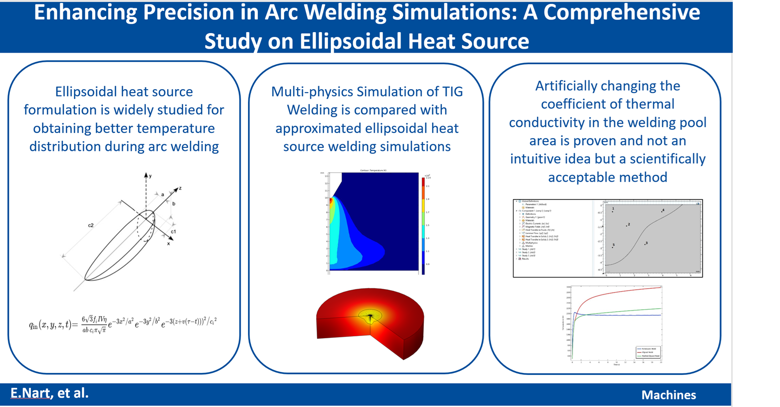
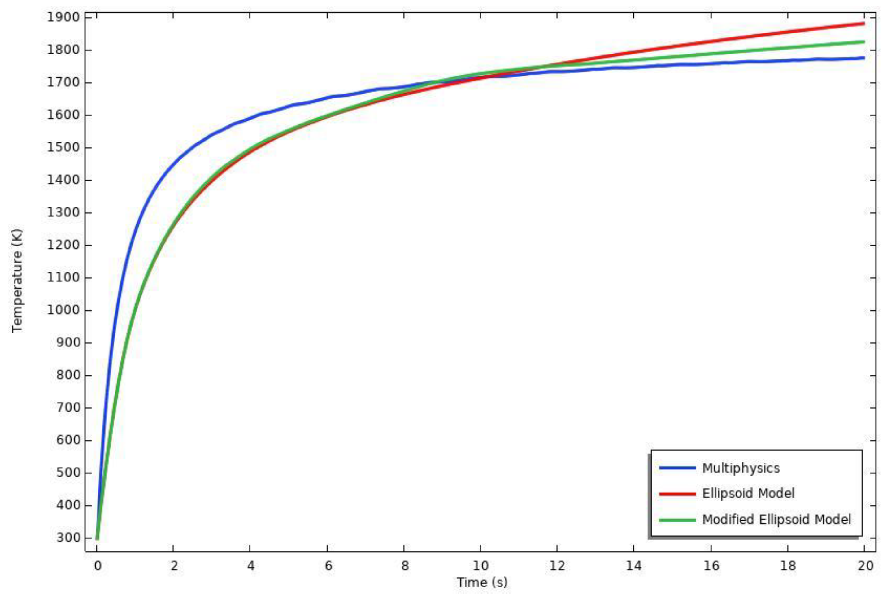
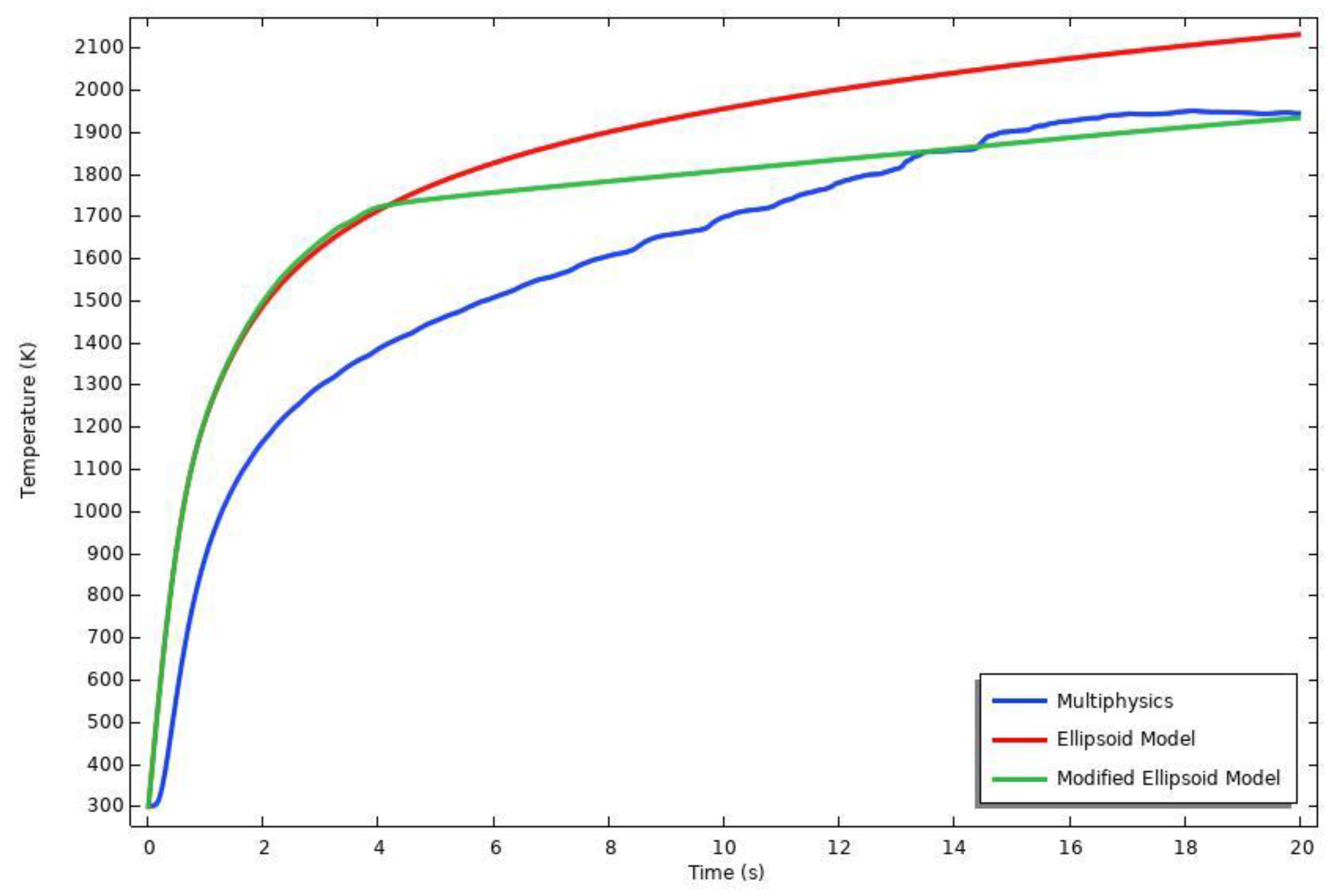
Arc welding is a complex multi-physics process, and its finite element simulation requires significant computational resources to determine temperature distributions in engineering problems accurately. Engineers and researchers aim to achieve reliable results from finite element analysis while minimizing computational costs. This research extensively studies the application of conventional ellipsoidal heat source formulation to obtain improved temperature distribution during arc welding for practical applications. Approximated ellipsoidal heat source model, which artificially modifies the coefficient of thermal conductivity in the welding pool area to simulate stirring effects, (Modified Ellipsoidal Model) is shown to be scientifically valid by comparing its results with those of Comsol's multi-physics arc welding models. The results show that, in comparison to the conventional ellipsoidal model, the temperature distributions obtained using the modified ellipsoidal model closely approach those from multi-physics simulations. In particular, the temperature history in the middle of the weld pool significantly changes and approaches the multiphysics solutions. Additionally, several points near the heat-affected zone were analyzed, and both ellipsoidal methods produced similar temperature histories until the metal melted. After melting, the modified ellipsoidal method gradually aligns more closely with the multiphysics solution. Additionally, both ellipsoidal methods produce similar temperature histories at points within the heat-affected zone.

Keywords: 
;  ;  ;  

1. Introduction

Since welding methods were invented in the early 1900s, these methods have been advanced and used for various materials in enormous engineering mitigation problems. In weld design applications, calculating the correct stress and temperature distribution in a welded part is very important. Therefore, engineers are eager to use every effective experimental and numerical method possible in the welding area. According to the historical perspective, it is true that the finite element (FE) is one of the most widely used numerical techniques in weld design analyses. Mainly, FE welding analysis can be performed in two ways. One way is a simple transient-thermal elastoplastic FE analysis, and the second way is a multi-physics analysis to determine the stress and temperature distribution in and around the weld region.
Up to now, several researchers, have investigated the Multi-physics welding phenomena intensively. Meanwhile, various commercial software is also available (Comsol Multiphysics, etc.) in the market, and they provide good results for even very complicated multi-physics cases in welding analyses. However, the multi-physics solutions require very big computational costs for even simple 2D analyses because FE analysis of the welding process consists of engineering disciplines such as Electricity, magnetism, CFD, Heat transfer, and solid structure in a couple each other. Additionally, in many large-scale steel construction areas, design engineers need much simpler FE models that require less computational cost unless they have very powerful computers. For this reason, searching for a simple and effective way of FE welding analysis goes back to the early 1980s.
In 1973, Udea et al. [1] showed that the FE procedures could be a couple or uncouple transient thermal elastic-plastic FE analysis. However, this kind of analysis model needs an appropriate heat source formulation to simulate the welding process. According to the literature, there are various heat source formulations proposed and used in FE welding analyses. If these heat source formulations are ordered from simple to complex ones, the first example can be the research done by Chau et al. [2]. In this research, authors propose uniform specific temperature usage not only for the weld bead region but also for a couple of surrounding regions in a regional way to simulate the process. Although the method employs a constant melting temperature distribution within the weld bead and the surrounding heat-affected zone to mitigate the severe temperature gradient, it fails to achieve an acceptable temperature distribution in the weld region.
Subsequently, Rosenthal [3] introduced a simplified point heat source model in 1946. While this formulation generally yields satisfactory results for areas sufficiently distant from the weld region, it predicts an infinite temperature at the source center, which is not physically realistic. To address this limitation, Pavelic et al. [4] proposed a Gaussian-distributed surface heat source model, offering improved accuracy in temperature distribution compared to Rosenthal’s model. However, this model is effective only in cases involving shallow weld penetrations, as the heat source is applied exclusively to the surface, thereby limiting its ability to model deeper welds.
Finally, Goldak et al. [5] introduced a significant advancement with a volumetric heat source model, which combines two ellipsoids representing the front and rear halves of the heat source. This double-ellipsoid model provides a more accurate representation of heat distribution within the weld region compared to earlier models and has been widely adopted by researchers and integrated into several commercial finite element software packages, becoming the de facto standard in the field.
Numerous good examples can be given from recent research. One of them is Koll´ar’s work [6]. In this research, the author deals with T-joints with fillet welds commonly used in civil engineering applications with Goldak’s method and investigates the impact of correcting the lack of penetration by repair welding concerning distortions and residual stresses. The research emphasizes the importance of the double ellipsoid method in welding simulation and avoiding repair welding by finding resultant plastic strain and von Mises residual stress increase significantly due to rewelding.
In a separate study conducted by Obeid O et al. [7], the authors examine the influence of girth welding materials on welded lined pipes through both numerical simulations and experimental investigations, incorporating a sensitivity analysis. Thermal and mechanical finite element (FE) models are developed using FORTRAN subroutines in conjunction with ABAQUS software, with pre-heat treatment conditions applied as initial parameters. In the experimental component, high-temperature strain gauges, residual stress gauges, and X-ray diffraction techniques are employed to measure strains and residual stresses along the inner and outer surfaces of the welded lined pipe. These measurements are correlated with the recorded thermal history to provide comprehensive insights into the welding process. However, these models have some weaknesses related to heat distribution in the weld region. Firstly, the weld pool’s shape must be ellipsoidal in this model. If the shape of the weld pool is non-ellipsoidal, the heat source equation must not be used properly. Secondly, the stirring phenomena in the molten metal flow occurring during welding are ignored. Therefore, especially in the weld fusion zone (FZ), if the temperature distribution is not determined as close as to reality. So, related residual stress calculations significantly deviate from the correct values as seen in reference [7] clearly in the weld pool region. Therefore, high-level calculations do not give good estimations such as ones in crack propagation inside Fusion Zone (FZ), which is highly important for providing the required safety, especially, in nuclear industries. Goldak et al. [5] recommend artificially increasing the heat conduction coefficient at nodal points where the temperature exceeds the melting point. However, this approach is insufficient to adjust heat distribution in the pool region to ensure all nodal temperatures reach the melting point. Nart et al. [8] proposed a new method of implementing Goldak’s heat source, replacing the previous nodal-based approach of increasing thermal conductivity in welding analysis with an area-based approach. According to the author’s research, the proposed approach shows an improvement in the history of temperature in FZ because the corresponding residual stress obtained from Finite Element simulation and X-ray measurement are very close to each other. Although the results of Nart’s work are meaningful, it is necessary to prove whether this experimental observation has a physical basis to proceed further.
Therefore, multiphysics welding models are closely investigated in this research. It is known that there are various kinds of research available that can be used to model welding phenomena realistically—some of these models in the literature deal with arc plasma modeling.
For example, Wu et al. [9] investigate plasma physics and its properties to optimize the performance of Tungsten Inert Gas (TIG) welding by simultaneously solving the conservation equations for mass, momentum, energy, and electric current. The authors develop a mathematical model to predict the distributions of velocity, temperature, and current density within argon welding arcs. Similarly, Hsu et al. [10] present solutions to the conservation equations for the entire free-burning arc, excluding the cathode and anode fall regions. The most critical boundary condition—current density near the cathode—is derived from measurements of the molten cathode tip size. The calculated temperature fields within the arc are validated through spectrometric measurements, utilizing both line and continuum intensity data from the arc.
These researchers focus exclusively on the arc plasma region to calculate the temperature distribution and gas velocity fields within the plasma. Their studies specifically investigate phenomena such as heat and current transfer, as well as the arc pressure and its associated drag force at the outer boundary near the weld pool. This targeted approach is essential, as arc welding phenomena cannot be accurately modeled when the arc plasma and molten pool are considered in isolation. Consequently, advanced models that integrate the conservation equations with selected Maxwell's equations, alongside appropriate boundary conditions, are required to more accurately represent Marangoni-driven flows.
For this reason, researchers have been extensively exploring new methodologies to model the multiphysics nature of the TIG welding process. Tanaka [11] investigates both the plasma and molten pool simultaneously, accounting for all the driving forces that influence convective currents within the molten pool during TIG welding. The study considers the drag force exerted by the plasma jet, the buoyancy force, the electromagnetic force generated by current flow in the molten pool, and the Marangoni effect, which arises from surface tension gradients. Tanaka's findings demonstrate that the formation of the molten pool is governed by the interplay of heat transfer and macro-convection within the molten region. Ultimately, the study concludes that the precise formation of the molten pool is dictated by a delicate balance among these four forces.
In another research paper, Tanaka et all [12] introduce a review of methodologies for predicting the properties of the arc and also the profile of the weld pool produced by the arc. The authors consider two electrodes in the modeling, i.e. cathode and anode, in which the electrode surfaces are needed in modeling for effects of energy and momentum transfer at the electrodes. The researchers also noticed that the temperature dependence of the surface tension coefficient has a marked effect on weld depth and profiles because it can influence the direction of circulatory flow in the weld pool. Tanaka et all, remarkably, realize that electric arc in different inert gases affects the weld pool shape as a consequence of the magnetic pinch pressure of the arc.
Tradia A. [13] in his dissertation studies mathematical modeling and numerical simulation of the arc welding process for both stationary and moving cases using GTAW. In the research, the author focuses on a 3D arc-welding model considering the welding position and the effect of the filler material used to investigate the GTAW process. The welding process is considered in pulsed current mode by using different gas mixtures, and the effect of welding parameters on the resulting weld shapes is investigated.
Recently, Yan Li et al. [14], the authors developed a useful method to calculate the keyhole PAW process with full consideration of multi-physical mechanisms. The paper investigates weld pool size with different solid viscosity and mushy zone constant. The model is useful to give a good prediction of weld pool geometry at proper welding conditions. The mathematical model was solved by the software Fluent with User-Defined Functions and User-Defined Scalar equations.
In this research, a dimensionally simplified multiphysics TIG welding model is implemented. It is well known that a multiphysics model for welding has several different partial differential equations to be solved simultaneously. This highly non-linear problem is very difficult to solve because the procedure cannot be computed in parallel computers. Therefore, axisymmetric finite element models can be used for as a special case for double-ellipsoid heat sources. However, the method used in this research must be extended to 3D welding problem to prove that modified double-ellipsoidal models can also provide engineers useful results.
In light of this, multiphysics TIG welding analysis is accordingly performed and the obtained results are compared with the results of the modified ellipsoidal heat source model. The work presented shows that approximated ellipsoidal heat source model with artificially changing the coefficient of thermal conductivity in the welding pool area is a scientifically acceptable method by comparing the results of both ellipsoidal approximate heat sources (Modified and conventional) and Comsol multi-physics arc welding model.

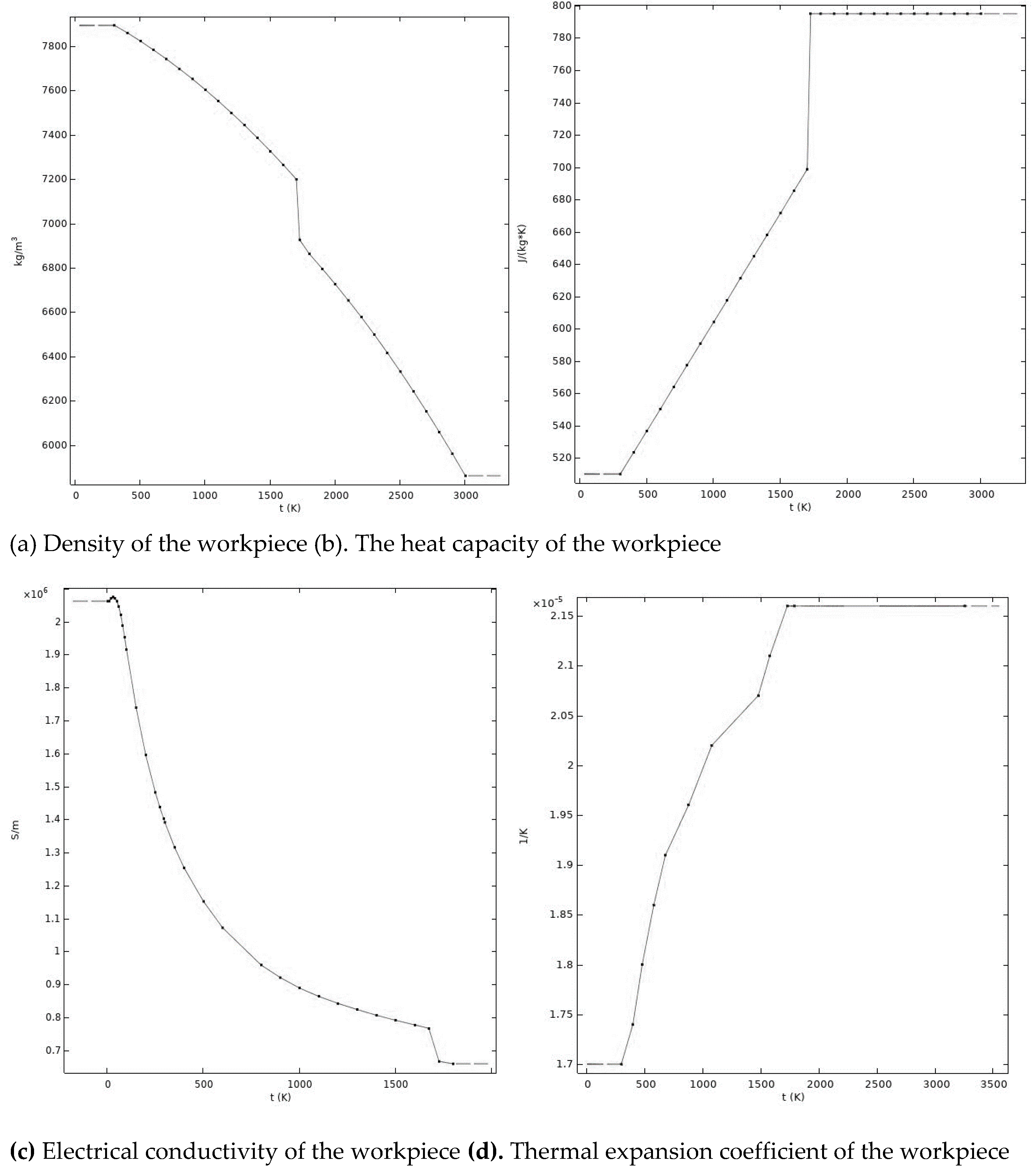
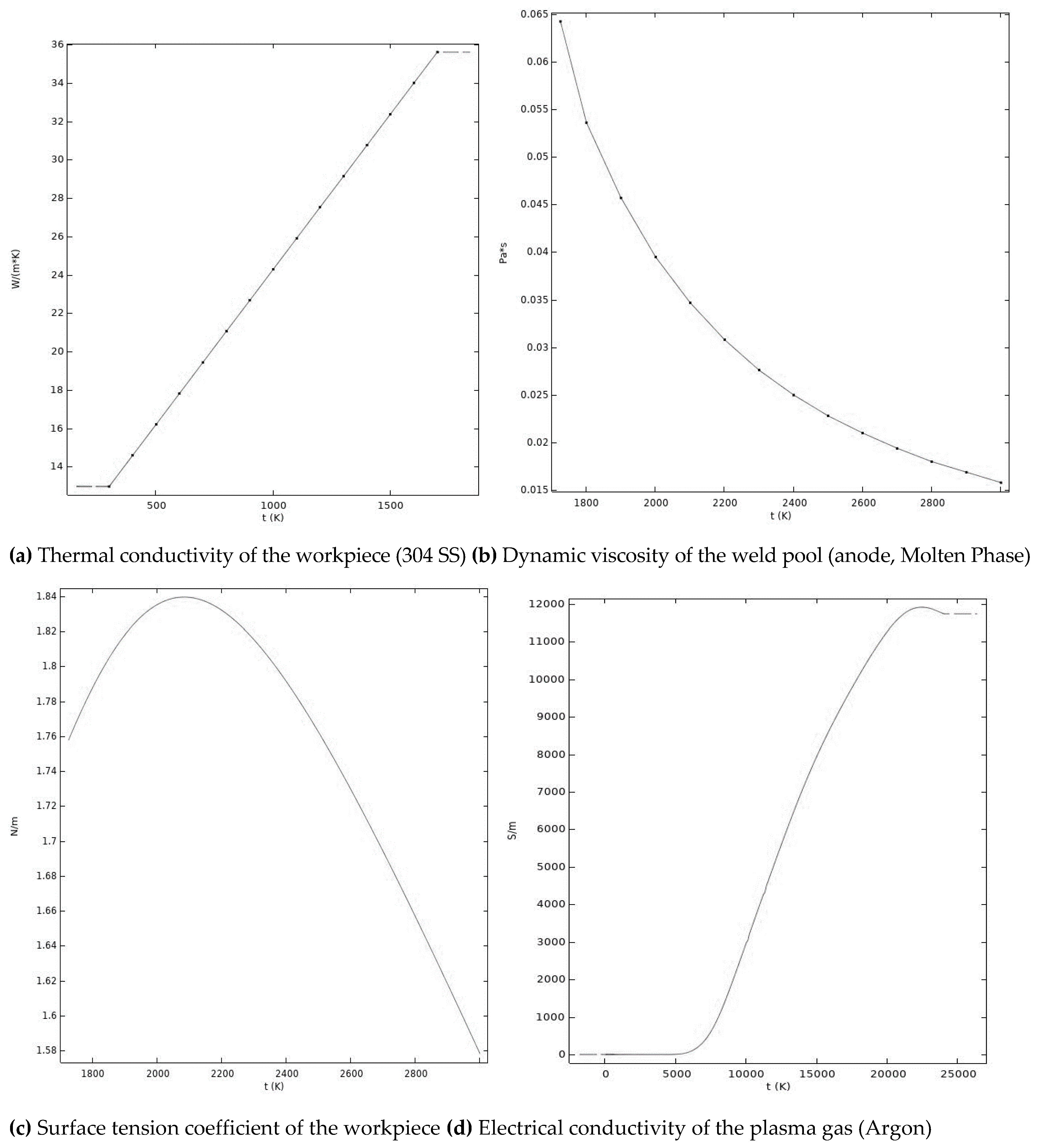
2. Mathematical Formulation and Governing Equations

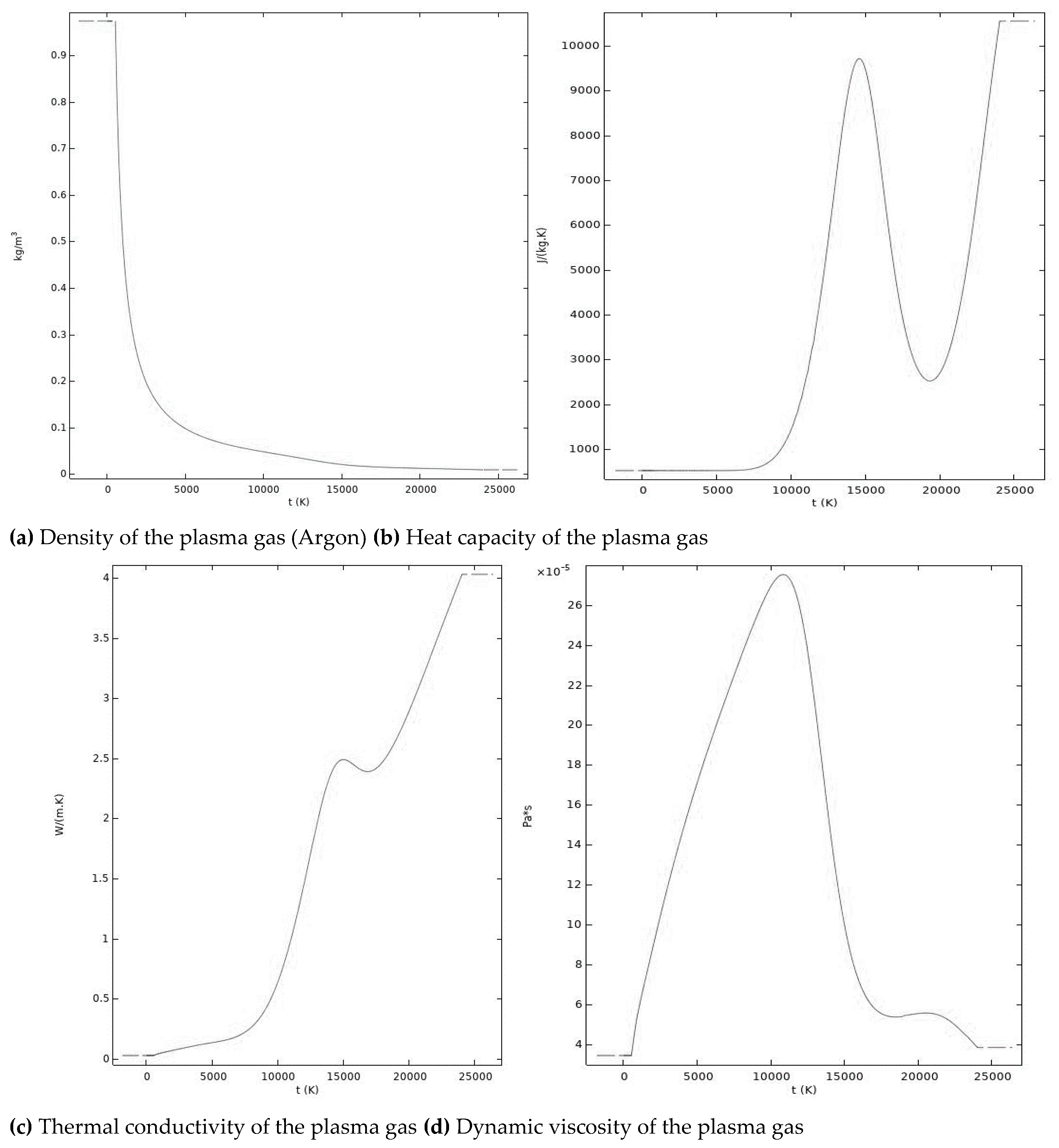
2.1. Equation for Thermal Plasma Modeling

Plasma is simply a superheated matter that is so hot that the electrons are ripped away from the atoms forming an ionized conductive fluid. Therefore, plasmas can be modeled using the magnetohydrodynamics (MHD) equations. It is well known that MHD uses the Navier-Stokes, heat, and Maxwell’s equations to define the motion of the conducting fluid in an electromagnetic field. After this, these governing equations determine the fluid motion of the plasma after solving in suitable manner. However, the plasma generated by the arc can reach high velocities due to thermal expansion and the electromagnetic forces acting on charged particles. The speed of the plasma can often exceed 0.3 Mach, particularly in the central regions of the arc where temperature and energy are highest. Consequently, these conditions within the arc can lead to compressible flow characteristics and deviations from Local Thermodynamic Equilibrium (LTE) in regions with strong velocity and density gradients. Similarly, other non-equilibrium conditions also occur in plasmas; for example, radiation emitted from the plasma disrupts the detailed balance as it escapes the plasma.
However, in high-temperature plasmas and rapidly moving gases, frequent collisions among particles can help maintain local equilibrium in small volumes, making the LTE assumption valid. This is possible because collisions allow particles to quickly share energy levels. On the other hand, concerning radiation processes, electrode heating from arc radiation can generally be ignored when a sufficiently high electron density is present. However, on the electrode surface, the cooling effect due to thermionic emission should be included in calculations.
In the field of welding, the LTE assumption is commonly used to model the behavior of the plasma arc. This approach allows for an approximate understanding of local thermodynamic properties to analyze heat transfer, melting processes, and the interaction between the arc and the workpiece. Additionally, the LTE assumption is typically employed as a starting point, enabling researchers to focus on primary interactions without getting overly involved in the complexities of non-equilibrium effects.
On the other hand, Although, the speed of the plasma can often exceed 0.3 Mach and this causes compressible flow in the arc-plasma, assuming incompressibility for plasma in welding arcs is often a reasonable approximation for simplifying the governing equations, and commonly used in theoretical models and simulations. For example, Lowke’s paper [22], “Simple theory of free-burning arcs”, presents an analytical framework to understand the behavior of free-burning arcs, which are commonly observed in welding and related plasma systems. The models in the paper incorporate simplified assumptions to make analytical solutions possible, such as considering steady-state conditions and approximations. Lowke et al find that in arc welding, when the arc current is relatively below 30 A, the inertia force associated with plasma become more relevant. At these lower currents, the plasma may exhibit noticeable motion due to inertia, which can influence the arc behavior.
However, as the current beyond 30A, the situation changes. The electromagnetics forces generated by the current (Lorenz force) become significantly stronger than the inertia forces. This is because the current generates a magnetic field that interacts with the plasma, exerting a force that tents to push the plasma along the arc. In the light of this knowledge, incompressibility for plasma in welding arc is a good opportunity to simplify the modelling.
Therefore, for the modeling of arc plasma in this research, the following assumptions are used [13];
Assumptions:
  • The arc is in Local thermodynamics equilibrium (LTE)
  • Axisymmetric Spot GTA welding is assumed
  • Pure argon is used and the metal vapors are not considered.
  • Gas plasma is incompressible and the flow is laminar.
  • Boussinesq approximation is not assumed in plasma.
Based on these assumptions, the conservation equations expressed in terms of axisymmetric case may be written as
v = 0   o r
1 r r r v r + z v z = 0
where v is the velocity vector, v r , and v z are the axial and radial velocity components, and ρ is the mass density, respectively. F V z and F V r represent the axial and radial volumetric forces. Additionally, the momentum equations are written as follows;
ρ v z t + ρ v z v z z + ρ v r v z r = p z + 2 z μ v z z + 1 r r μ r v z r + 1 r r μ r v r z + F V z
ρ v r t + ρ v z v r z + ρ v r v r r = p r + z μ v r z + 2 r r μ r v r r + z μ v z r 2 μ v r r 2 + F V r
And, in the plasma region, the axial volumetric force is defined as the sum of Lorentz and inertia force:
F V z = J r B θ + ρ 0 g
in which ρ 0 is the gas density and the gravity force is included for taking into account the action of buoyancy in the arc plasma domain, Also, the radial volumetric force is the Lorentz force [4] and defined as;
F V r = J z B θ
In these equations, p, μ , Jr , Jz , and Bθ are the pressure, the viscosity, the radial and axial current density, and the self-magnetic field, respectively [13]. Above equation (3), the self-induced magnetic field can be written as
B θ = 0 r μ 0 r J z r d r
There is another way to obtain B θ that is used in Comsol. Magnetic potential equations are
A r t + 1 r r r A r r + z r A r z = μ 0 J r A r r 2
A z t + 1 r r r A z r + z r A z z = μ 0 J z
B θ = A r z A z r
After, the current continuity equation is simply obtained from Gauss’s law;
J z z + 1 r r r J r = 0
or
J = 0
and formulated as a function of the electric potential φ as follows;
z σ φ z + 1 r r σ r φ r = 0
or
σ 2 φ = 0
where σ is the electrical conductivity. Ohm’s law yields
J r = σ φ r , J z = σ φ z
Finally, the energy conservation equation takes the form;
ρ C p T t + v r T r + v z T z = 1 r r k r T r + z k T z + S v
But, in the plasma region, the volumetric heat source consists of the Joule effect, the electrons enthalpy ( 5 2 k B e J T ) , and the radiation losses:
S v = J z 2 + J r 2 σ + 5 2 k B e × J z T z + J r T r Q r a d
where T, Cp, k, kB, e, and S v are temperature, specific heat at constant pressure, thermal conductivity constant, the Boltzmann constant, elementary charge, and volumetric heat sources respectively. Additionally, Q r a d is the approximated radiation loss taken as 4πЄN, where ЄN is the argon’s net emission coefficient changing with temperature.
Furthermore, the energy equation consists of convection, conduction, joule-heating, and electron enthalpy terms (because of electron-ion collision in the anode). Corresponding coupled governing equations are highly nonlinear systems of partial differential equations and the solution is reached by solving them simultaneously.
In this research, Comsol software is used to model and solve these equations by using its strong multiphysics features. In the Comsol environment, one can define all partial differential equations and boundary conditions, and make proper connections among them in couple to solve problems. On the other hand, various interfaces can be easily used in Multiphysics modeling and simulations. For instance, the Magnetic Fields interface can be used to solve Ampère’s law. Then, The Equilibrium DC Discharge interface can be employed to analyze equilibrium discharges induced by static or slowly varying electric fields. This interface operates under the assumptions that the plasma is fully ionized, in a state of local thermodynamic equilibrium (LTE), and that induction currents are negligible. In addition, the Equilibrium Inductively Coupled Plasma interface is designed to evaluate equilibrium discharges resulting from induction currents, as observed in inductively coupled plasma torches. Alternatively, the Combined Inductive/DC Discharge interface facilitates the assessment of equilibrium discharges arising from both induction currents and static or slowly varying electric fields, making it particularly suitable for applications such as arc welding simulations. For thermal and fluid dynamics analyses, the Heat Transfer and Laminar Flow interfaces are available to solve the energy equation and the Navier-Stokes equations, respectively. Importantly, multiphysics coupling terms play a critical role in effectively linking these equations, ensuring accurate simulation of the interdependent physical phenomena.

Electrode and Anode Surfaces

Meanwhile, the positive ions within the plasma contribute to heat generation at the electrode surface. As the electrode temperature rises, an increased number of electrons are emitted via thermionic emission, leading to a cooling effect on the cathode. Consequently, for points along the electrode surface, it is essential to account for both the cooling effect induced by thermionic emission and the heating effects resulting from ion current and thermal conduction in the calculations. It is assumed that the heating of the electrodes due to arc radiation is negligible. For the cathode, the additional energy flux to the electrode, denoted as FElectrode, is expressed as:
F E l e c t r o d e = ε α T 4 j e ϕ K   + j i V i
where ε is the emissivity of the surface, T is the surface temperature, ϕ is the work function, j e is the electron current density, j i is the ion current density, α is the Stefan-Boltzmann constant, V i is the ionization potential of the plasma [17].
where ε represents the emissivity of the electrode surface, T denotes the surface temperature, ϕ is the work function of the material, j e and j i correspond to the electron and ion current densities, respectively, α is the Stefan-Boltzmann constant, and V i signifies the ionization potential of the plasma [17].
The ion current density norm is defined by:
j i = j . n j e
where j . n is the normal current density at the interface and where
j e = j R , i f   j . n > j R j . n ,   i f   j . n j R
is the electron current density norm. The latter is defined by Richardson-Dushman current density if the total normal current density is larger than
j R = A R T 2 e x p ( e ϕ e f f k b T )
here j R denotes Richardson’s constant, e represents the elementary electronic charge (C), k b is Boltzmann’s constant, and ϕ e f f corresponds to the effective work function of the surface. It is important to note that the ion current density, j i becomes zero if the Richardson-Dushman current density exceeds the total normal current at the interface [18]. At the anode surface, the sign of the term j e ϕ in Equation (11) is reversed to reflect the positive heating effect associated with electrons absorbed at the anode. In this context, ϕ represents the work function of the anode material.
The anode, typically represented by the workpiece, constitutes a distinct region within the arc plasma due to its function in receiving electrons emitted from the cathode. This relatively thin layer operates as an electron-absorbing zone, thereby maintaining electrical continuity between the workpiece and the arc column. As electrons are emitted from the cathode and subsequently accelerated through the arc column, they collide with the anode surface, transferring their kinetic energy to the workpiece. This process is known as electron condensation heating, and it contributes significantly to the thermal energy input of the workpiece through both the arc plasma and the incident electron flux.
However, with regard to radiative effects, the heating of the anode due to arc radiation can generally be considered negligible. Studies in the literature report that the contribution of radiative heat flux to the anode constitutes less than 5% of the total heat input. Nonetheless, for accurate thermal modeling of the anode surface, it is essential to incorporate the cooling effects resulting from thermionic emission into the calculations.
For this reason, the additional energy flux, FAnode, to the anode is taken as
F A n o d e = ε α T 4 + j e ϕ A
Under the assumption of Local Thermodynamic Equilibrium (LTE), the electron density is equal to the total density of positive charges, thereby maintaining charge neutrality. On the other hand, the presence of electrodes introduces effects that cause local imbalances between negative and positive charges, leading to non-LTE conditions. When the regions near the anode surface are very thin, which is approximately 1.5 μm in a 200 A-argon arc, non-equilibrium conditions in charge densities occurs.

2.2. Equation for Weld Pool Modeling

The fluid flow occurring in the anode region is defined by the conventional conservation equations of mass and momentum. These conservation equations can be written in a time-independent form in eq. (16,17,18) with respect to the assumptions given below. In addition, the solution for the electromagnetic problem in the anode and cathode domain is needed to calculate the Lorentz forces and the Joule effects for heating. These Lorentz forces and the Joule effects for heating are governed by the classical Maxwell's equations given previously.
Assumptions:
  • Axisymmetric Spot GTA welding is assumed
  • Metal flow in weld pool is laminar.
  • The surface tension coefficient is dependent on both temperature and sulfur content.
  • The latent heat of fusion is also taken into account.
  • Boussinesq approximation is assumed in weld pool.
The conservation equations for weld pool is
v = 0 1 r r r v r + z v z = 0
The momentum equations are
ρ v z t + ρ v z v z z + ρ v r v z r = p z + 2 z μ v z z + 1 r r μ r v z r + 1 r r μ r v r z + F V z
ρ v r t + ρ v z v r z + ρ v r v r r =
p r + z μ v r z + 2 r r μ r v r r + z μ v z r 2 μ v r r 2 + F V r + F A
In the anode region at liquid phase (weld pool), the axial volumetric force consists of Lorentz and inertia force, and the buoyancy force
F v z = J r B θ + ρ 0 g ρ 0 g β ( T T l )
In the above equations, ρ 0 is the melted metal density in the weld pool as the reference. The radial volumetric force is the Lorentz force:
F v r = J z B θ
Additionally, two more sources of radial momentum exist at the liquid surface of the weld pool. The first is the drag force caused by the shear stress due to the convective flow of the cathode jet on the surface of the weld pool. This drag force is already included in Eq. (18) through the viscosity at the weld pool surface. The second is the Marangoni effect due to the gradient in the surface tension at the surface of the weld pool. This force usually occurs due to temperature differences between the center of the weld pool and the edge of the weld pool. Moreover, these effects can also occur due to changes in the chemical composition of the liquid steel. The additional term for Eq. (18) at the weld pool surface F A is:
F A = z d γ d T T r
The temperature coefficient of surface tension, d γ d T , for pure metals is typically negative. However, the presence of impurities such as sulfur in the weld pool can alter this coefficient, resulting in a positive d γ d T value. In cases where d γ d T is positive, the direction of the surface stress induced by the Marangoni effect is reversed, leading to significant changes in the flow dynamics within the weld pool. This alteration in surface tension-driven flow subsequently influences the geometry and morphology of the weld pool.
In invaluable research, Sahoo et al. [15] show that the surface tension γ as a function of both temperature and sulfur activity is obtained as:
γ = γ m o A γ ( T T m ) R g T Γ s l n 1 + k 1 a i e ( Δ H o R g )
differentiating Eq. (22) with respect to temperature, the expression of d γ d T as a function of both temperature and sulfur activity can be written as:
K = k 1 e ( Δ H o R g )
d γ d T = A γ R g Γ s l n 1 + K a i K a i 1 + K a i Γ s Δ H o T
The related values for coefficients are given in Table 1. Also, the terms in the energy conservation equation are expanded for the anode (workpiece) and cathode region (electrode), the volumetric heat source term consists of the Joule effect and the radiation losses:
S v = J E Q r a d
In the same equation, Q r a d is another term for the radiation loss;
Q r a d = ε α T 4
where ε is the emissivity of the surface, T is the surface temperature, α is the Stefan-Boltzmann constant. Also, c p e q is an equivalent specific heat, that is correspond to c p in the arc-plasma and cathode regions, and is recalculated for the workpiece (anode) domain taking into account of the latent heat of fusion L f :
c p e q = c p + L f ( f L t )
In the meantime, a linear change with temperature is assumed for the liquid fraction fL as follows [19]:
f L = 1 ; i f T > T L
f L = T T s T L T s ; i f T s > T L
f L = 0 ; i f T < T L
where TS and TL are solidus and liquidus temperatures of metal respectively. The variables and constants with units are given in Table 2.

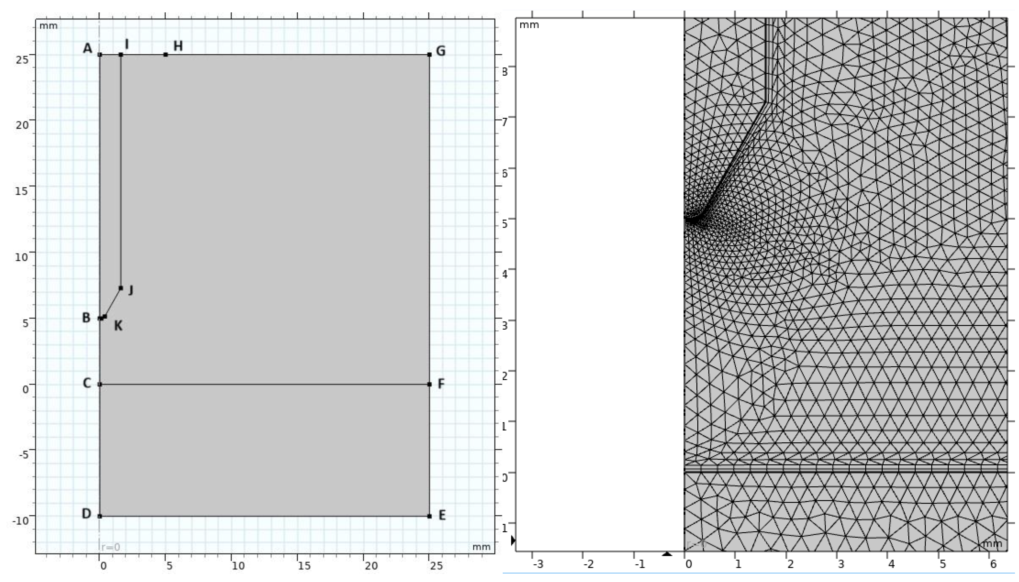
3. Computational Domain and Initial Conditions

To define the corresponding domains for governing equations and suitable boundary conditions for this research, the geometry is divided into three subdomains with different mesh densities in each one (Figure 1). For this reason, ABKJI, CDEF, and BCFGHI polygons are formed for cathode (tungsten electrode tip angel 60-deg), anode (304 stainless steel– medium sulfur content), and arc-plasma regions respectively.
For the arc-plasma part of the problem, the temperature distribution is computed in the arc-plasma and anode domains, however, the fluid flow is computed in the arc-plasma domain only [10].
For the weld pool part of the problem, the electromagnetic, energy conservation, mass and momentum conservation equations are solved in the workpiece domain CFED. Also, all required boundary conditions are given in Table 3.

3.1. The Free Surface Deformation

Because of the arc pressure, surface tension and gravitational force acting on the weld pool, the linear form is lost on the free surface of melted metal in the weld pool. The arc voltage and welding current directly affect the degree of this related deformation Therefore, the behavior of the liquid/solid interface should be investigated more closely and necessary assumptions should be made properly. For this reason, according to the research conducted by Ushio et al. [16], it is concluded that the free surface deformation occurs reasonably small in the course of the process with respect to that of other welding processes. Therefore, it is assumed that the free surface is flat for all MHD calculations.

3.2. The Liquid/Surface Interface

Within the welding pool, an additional interface exists between the liquid and solid phases of the metal. This liquid/solid interface is typically defined by the contour corresponding to the liquidus temperature. Methods employed in weld pool simulations to account for this interface are generally classified into two categories: moving grid methods and fixed grid methods. In the fixed grid approach, the mesh for the pool domain is generated once, and the liquid/solid interface is determined using the liquid fraction function, fL(T). Since the momentum equation is solved across the entire domain, it is necessary to ensure that the velocity field remains zero in the solid region. To achieve this, the Karman-Kozeny approximation and the enhanced viscosity method are commonly applied. In the present study, the enhanced viscosity method is utilized, as described in Equation (28).
  μ = μ L ( T ) f L + μ S ( 1 f L )
In the moving grid methods, the interface for liquid/solid is tracked with time to generate two distinct sub-regions for the melted and solid metal zones at each time step.

3.3. Initial Conditions in Arc Plasma Region

An electric arc is fundamentally a form of electrical discharge initiated through ionization when the current across the electrodes exceeds the breakdown voltage. This critical breakdown voltage across the electrode gap is influenced by factors such as the surrounding gas pressure, the inter-electrode distance, and the type of gas present. Typically, an electric arc is initiated by bringing two electrodes into contact and then gradually separating them. The electrical resistance along the resulting continuous arc generates heat, which further ionizes surrounding gas molecules, progressively transforming the gas into a thermal plasma. This mechanism allows for the initiation of an arc without requiring a high-voltage discharge. A similar process occurs during welding, where the welder briefly touches the welding electrode to the workpiece before withdrawing it to establish a stable arc. However, the physical actions of touching and withdrawing electrodes cannot be directly modeled within a fixed mesh computational domain. To address this limitation, an appropriate numerical modeling technique must be employed. This is achieved by imposing a numerically conductive channel between the electrodes. The variation in electrical conductivity within this channel can be effectively represented using an exponential decay function, which facilitates the accurate simulation of arc initiation by defining:
σ t = 0 = A exp B r S m
In this way, artificially, electrical conductivity at r=0 is increased and the arc is initiated for suitable constant values of A and B.

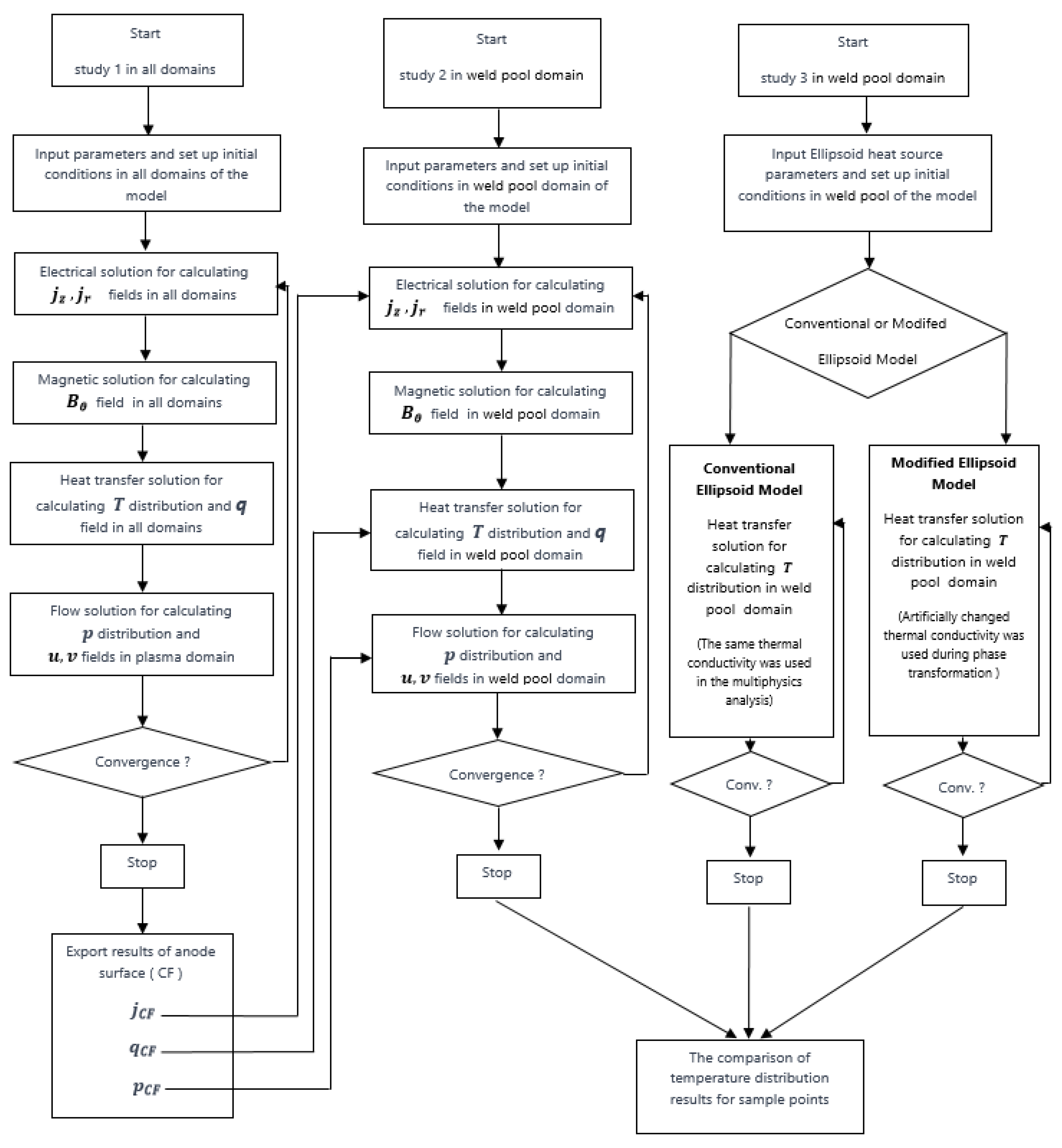
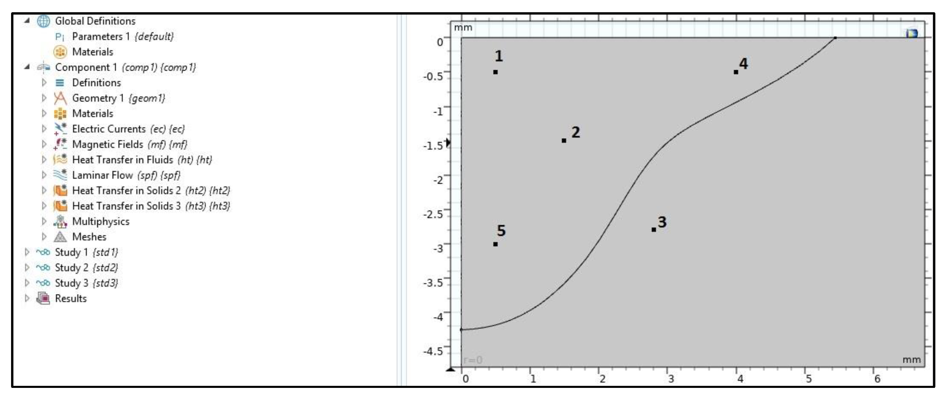
4. Implementation in Comsol

Comsol software is utilized to solve all couple governing equations modelled the multiphysics arc welding problem. For this reason, all the governing equations are defined by suitable components with their multiphysics couplings and interfaces. Mainly, the overall simulation procedure can be summarized as follows. In each time increment, the magnetic and electric potentials are computed primarily in the whole domain. Then the electric field, current density and magnetic induction are calculated. Next, for calculating the related temperature field, the Joule heat source values are used.
Thus, resulting velocity and pressure are determined using the previously obtained Lorentz forces and thermal field. If the convergence criteria are not acceptable, all temperature-dependent properties are updated by using the current temperatures, and these steps are repeated until the required convergence is reached. All material properties used in multiphysics analysis are given in Figure 2, Figure 3 and Figure 4 and Table 4. Detailed Comsol solution procedures are given in Figure 5.
For the ellipsoid heat source model in Comsol, the formulae used have Gaussian distribution form of the power density as given in Eq.30. In this equation, q ( 0 ) represents the maximum value of the power density at the center of the ellipsoid. In this heat source modeling, the power is separated into two halves that consist of front and rear quadrants. the power for two halves is calculated by integrating as in Eq.31.
q ( x , y , z ) = q ( 0 ) e A x 2 e B y 2 e C z 2
2 Q = 2 η V I = 8 0 π / 2 0 0 q ( 0 ) e A r 2 e C z 2 r d r d z d θ = q 0 π π   A C
According to the boundary conditions
q a , 0 = q 0 e A a 2 = 0.05 q 0
q 0 , c = q 0 e C c 2 = 0.05 q 0
coefficients of heat flux are found as;
A 3 a 2   C 3 c 2
Finally, power density distribution inside the front and rear quadrants becomes:
q f r , z = η 6 3 V I a 2 c π π e 3 r 2 a 2 . e 3 z 2 c 2 q r r , z = η 6 3 V I a 2 c π π e 3 r 2 a 2 . e 3 z 2 c 2
Throughout ellipsoid heat source analyses, the parameters are used as follows: I=150 Amp V=12 Volt, a=4.25mm and b=5.40mm
Meanwhile, it should be noted that artificially changing the thermal conductivity is a concept that can be implemented in Finite Element Analysis in different ways. Especially in 2D problems (depending on the welding speed), when the torch arrives at the observation section, thermal conductivity is changed to a specific value in the whole area of FZ. This artificially changing the thermal conductivity gives good results as reported in reference [8]. In this research, the problem is modeled in an axisymmetric domain, as the elements in the fusion zone start growing from a point to a certain melted pool size (depending on the parameters used), and all elements within the melted pool are exposed to artificially increased thermal conductivity. The value of the stirring thermal conductivity is taken at 120W/m2C as indicated in reference [5]. In Comsol, this is easily implemented by using phase change calculations in the weld pool regi

5. Results and Discussion

All results obtained during this research can be summarized in three main stages. In the first stage, the arc plasma model is presented. Because the arc plasma inputs are the most important aspects of an arc welding simulation, related results are carefully validated with a well-known reference. In the second stage, the modeling of molten metal flow during GTA welding is fulfilled by implementing well-known formulae for surface tension concerning temperature and sulfur concentration. Then, several points are selected from the melted pool region to obtain multiphysics thermal histories. In the last stage, a comparison of multiphysics, conventional and modified ellipsoid models is done correspondingly.

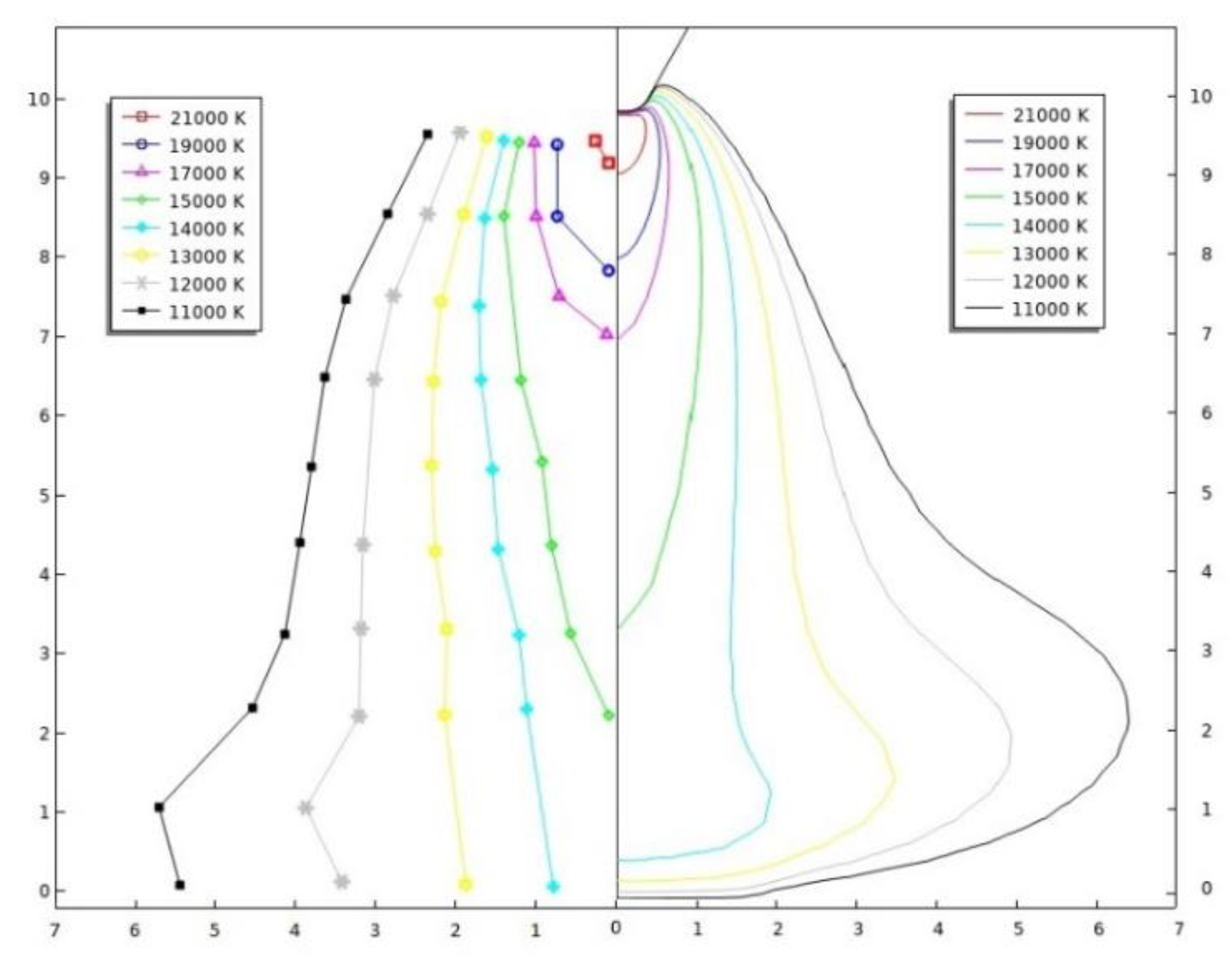
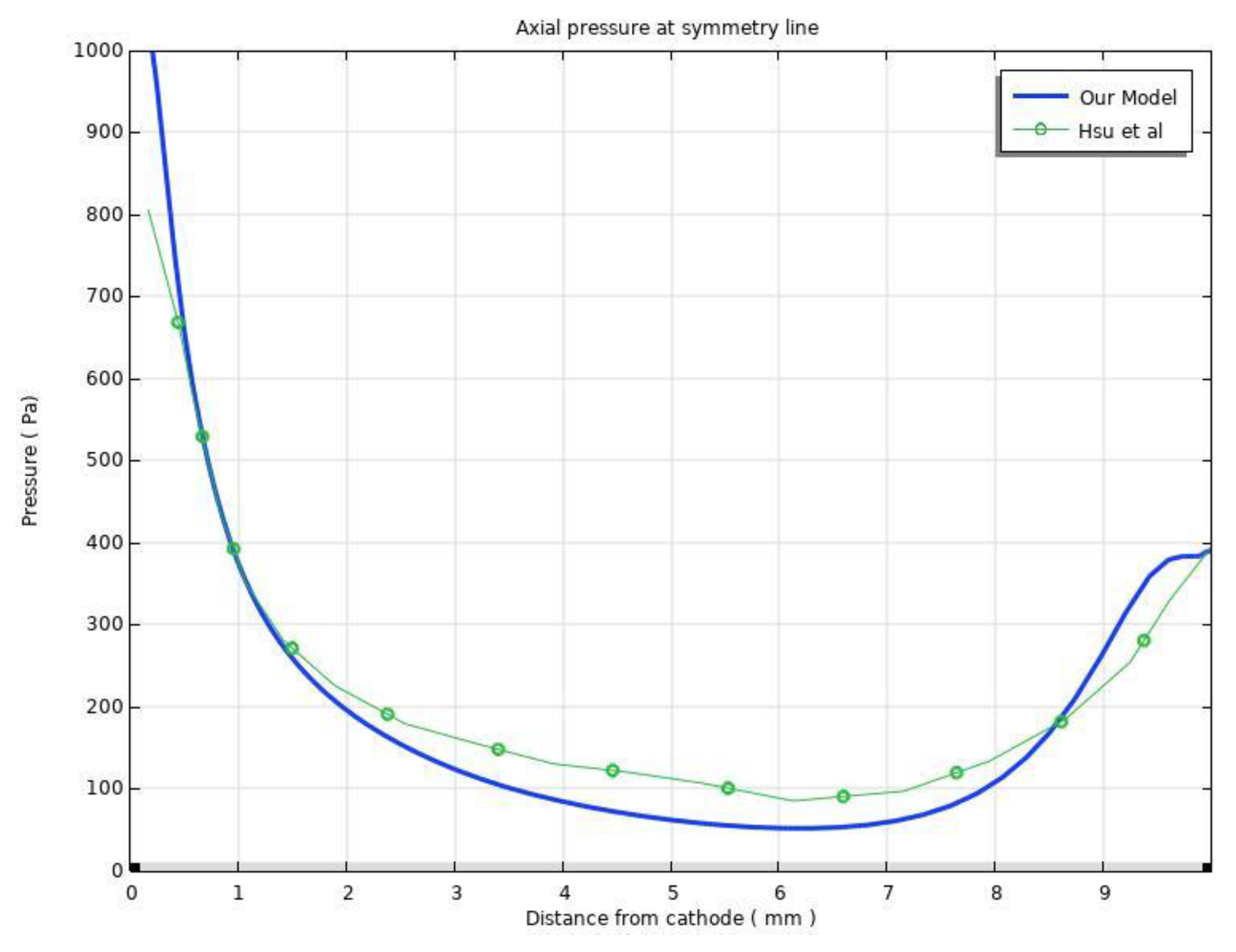
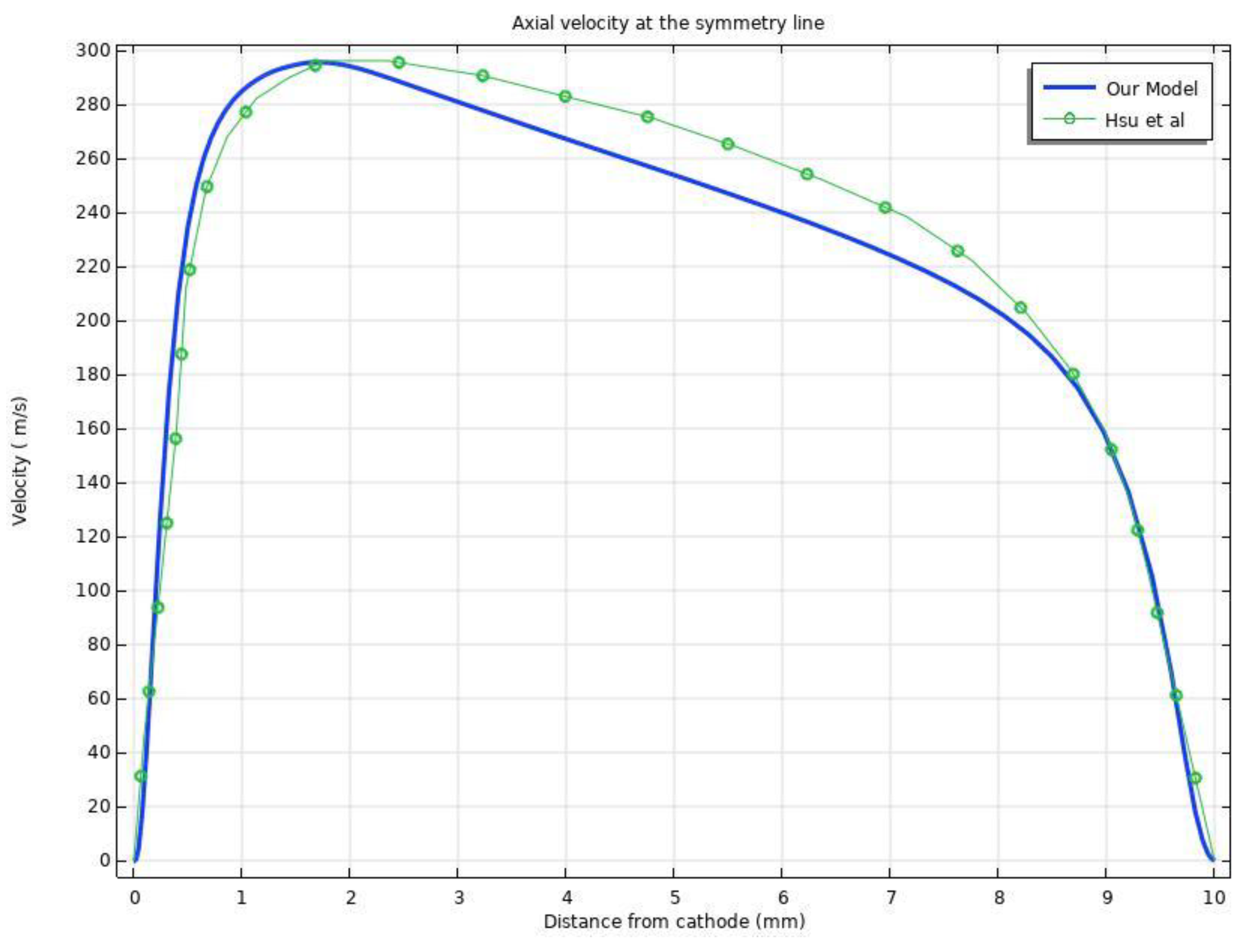
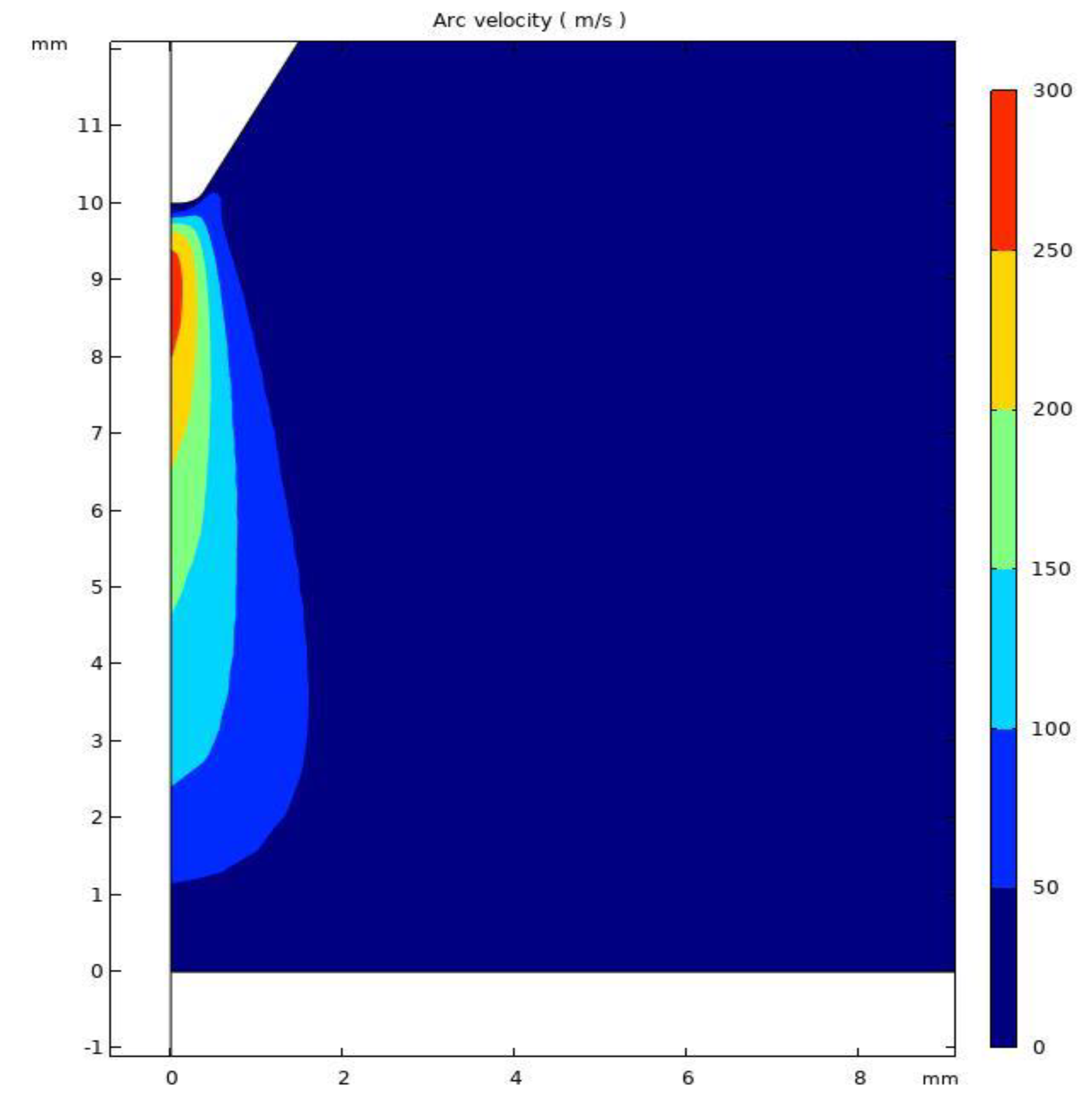
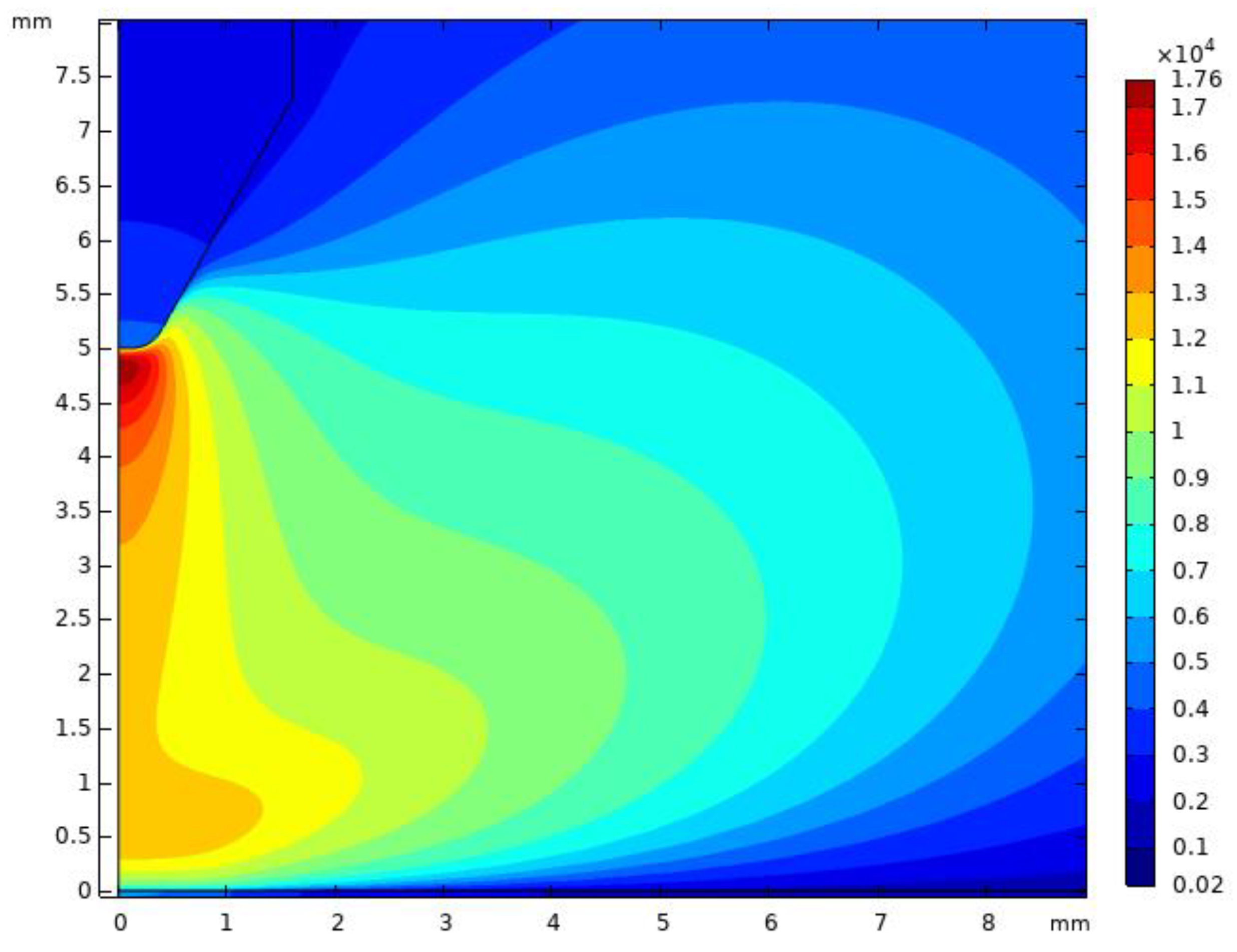
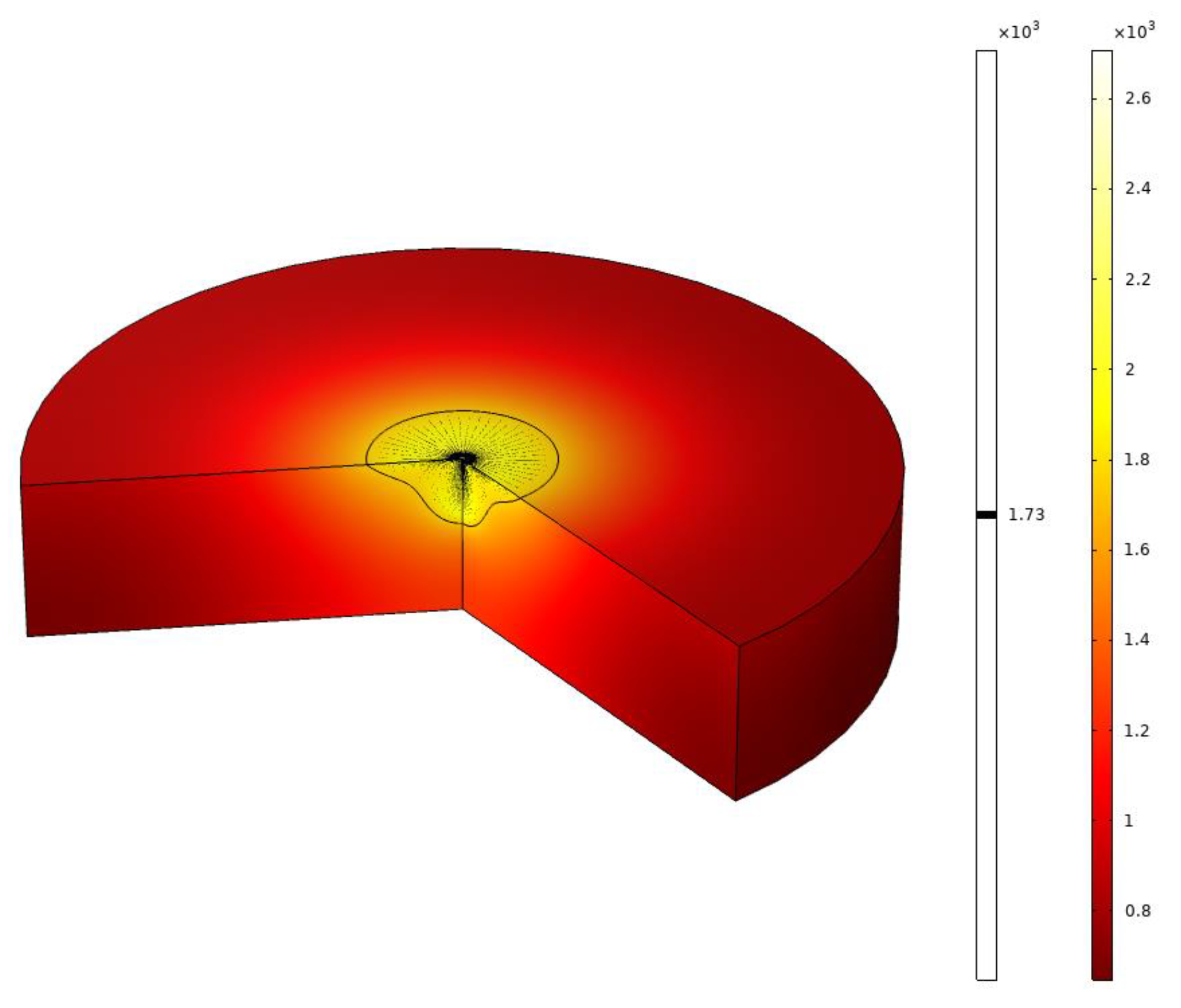
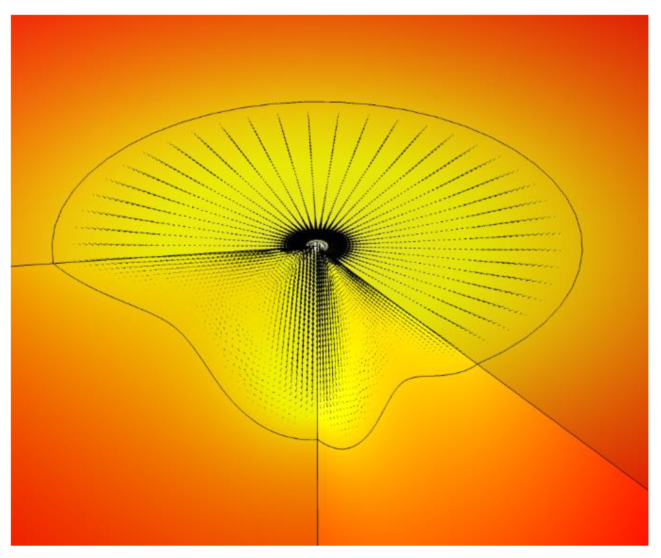
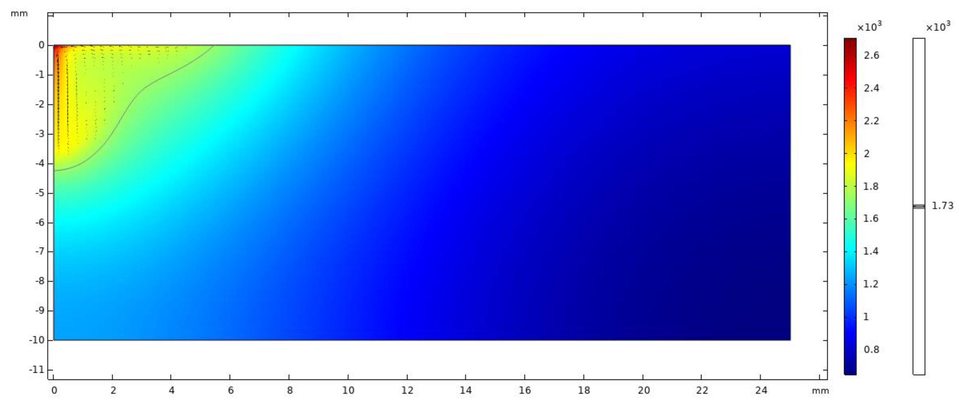
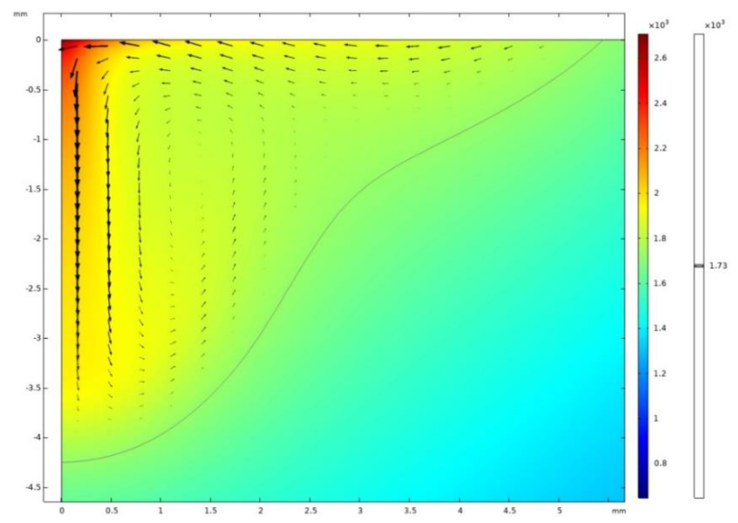
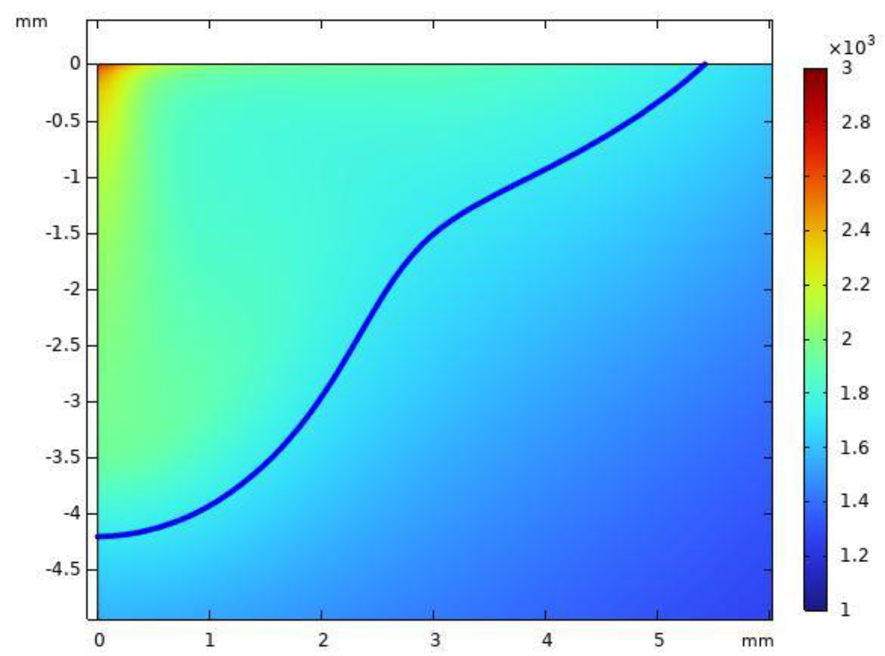
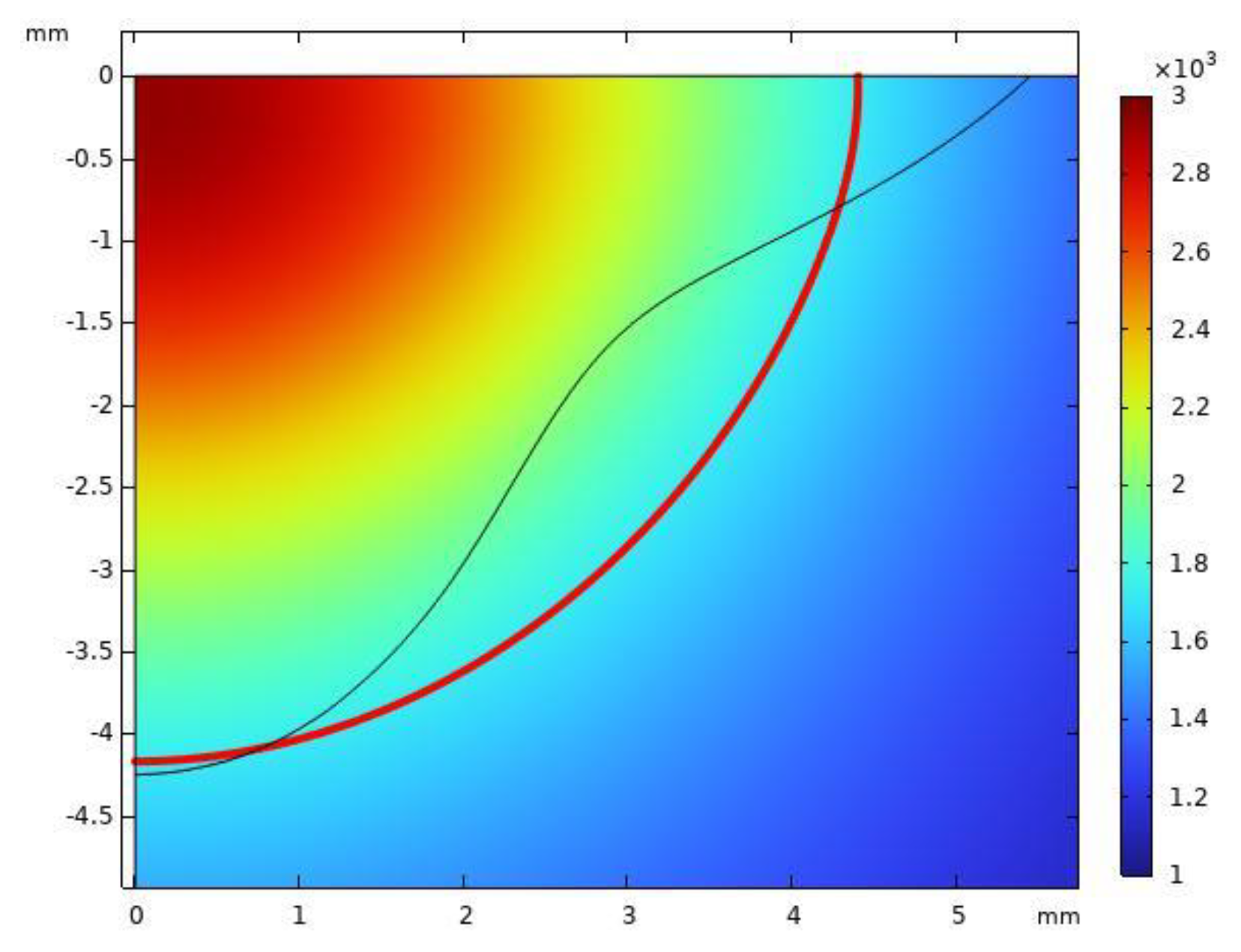
5.1. Plasma Model Results and Validation

In the plasma validation process, the Comsol model, used in this work is simply modified according to the dimensions and welding parameters taken from Hsu’s research work [Hsu] ( I=200A, BC=10mm). The obtained results are compared with that of Hsu’s research.
In Figure 6, it can be seen that similar results are obtained even though Hsu et al. assume that on the anode surface (CF), the temperature distribution is taken experimentally, and at the boundary GF, the temperature of 1000 K is postulated.
In Figure 7, the temperature exhibits a rapid increase in front of the cathode due to Ohmic heating, and as the arc spreads (decrease of the current density), the temperature drops to values below 15 000 K close to the anode. As seen in Figure 8, A big pressure change takes place near the cathode tip because the strong electromagnetic force occurs due to the high current density around. However, it decreases rapidly as getting away from the cathode (electrode). Additionally, when the pressure effect vertically reaches the surface of the workpiece (anode), there is an increase in pressure because of the gas-wall impact effect.
In Figure 9. The axial velocity rises to a maximum at the electrode tip due to the strong pressure difference; the axial velocity decreases rapidly as approaches the workpiece and becomes zero. In Figure 10, the contour plot of velocity distribution is shown.

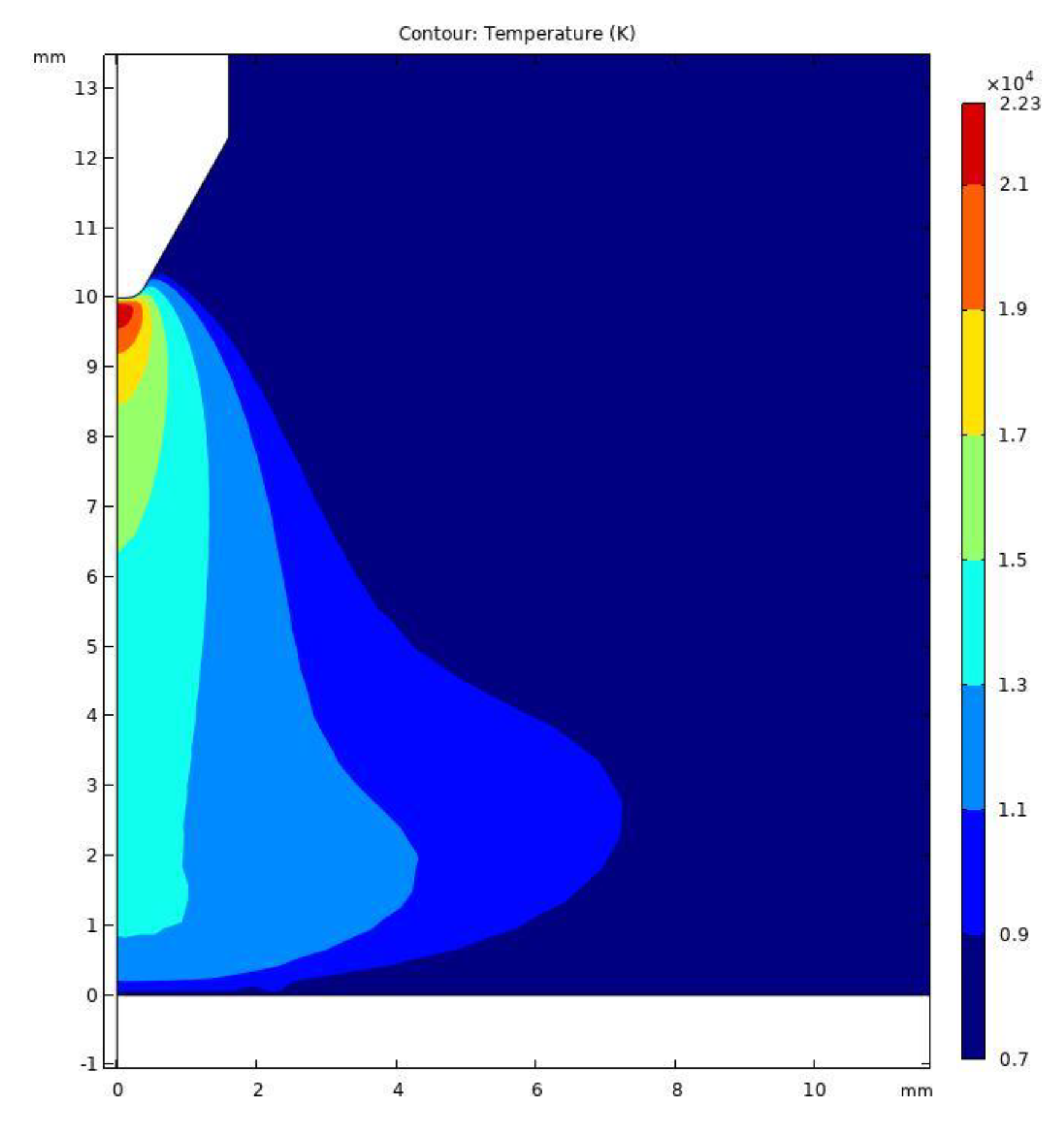
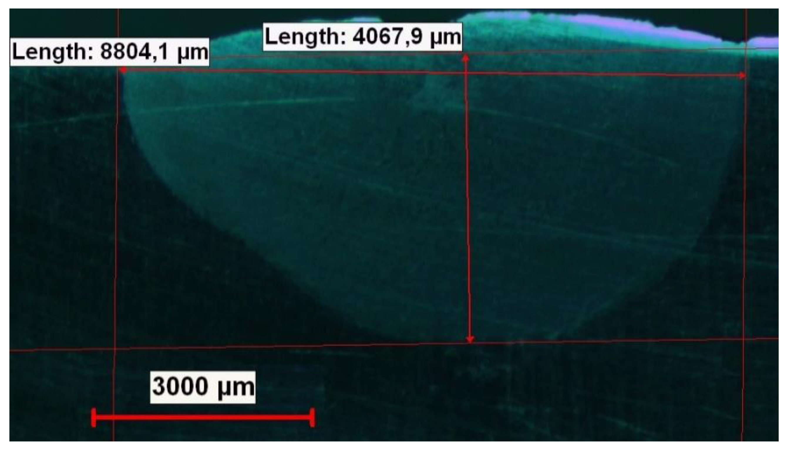
5.2. Weld Pool Results and Validation

The multiphysics model results need validation to go further in this research. To validate the multiphysics solution procedure developed in this research, the research by Tanaka et al [21] is selected. In Tanaka’s study, the authors give calculations of the time-dependent two-dimensional asymmetrical distributions of temperature and velocity in a whole region of the welding process.
Accordingly, the authors also provide experimental results in their paper. Therefore, the same model with the same boundaries, definitions, and parameters is constructed in Comsol software for validation, and corresponding results are obtained.
In Figure 11, it can be seen that electric arc plasma formation is obtained from the corresponding Comsol model. If the related results are used as input in the modeling of molten metal flow in the GTA welding process, the weld pool problem is solved and a corresponding temperature and melted metal flow solutions are obtained. According to the results achieved, it is observed that a liquid with a high surface tension makes the surrounding liquid with a low surface tension move strongly. Expectedly, Marangoni convection dominates the fluid flow in the weld pool due to the temperature gradient of surface tension.
In Figure 12 and Figure 13, temperature and velocity distribution in the weld pool region can be seen in the 3D view of axisymmetric results. Accordingly, if the results in the welding region appear in cross-sectional views, at the right part of the weld cross-section in Figure 14 and Figure 15, two vortices can be seen in the weld pool; the first one is a counter-clockwise vortex near the center of the weld pool forming an inward fluid flow at the surface, and the second one is clockwise vortex near the edges of the weld pool forming an outward fluid flow. It can be seen that the first counterclockwise vortex is visibly leading and forms a deep and narrow weld pool. However, the second clockwise vortex induces a wide and shallow weld pool.
In the validation part of this research, it is clear in Table 5 that the Comsol model used in our study gives similar results to those in Tanaka et al’s results. Both simulations are very close to the experimental result presented in the reference [21]. Additionally, authors also performed an experiment to validate Tanaka’s results using same welding parameters. As show in Figure 16, at least, the pool sizes are found to be almost close to Tanaka’s results.

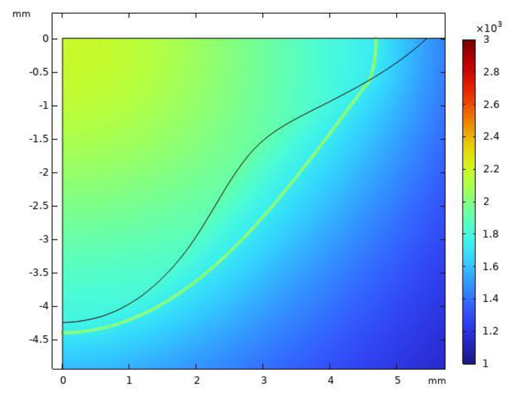
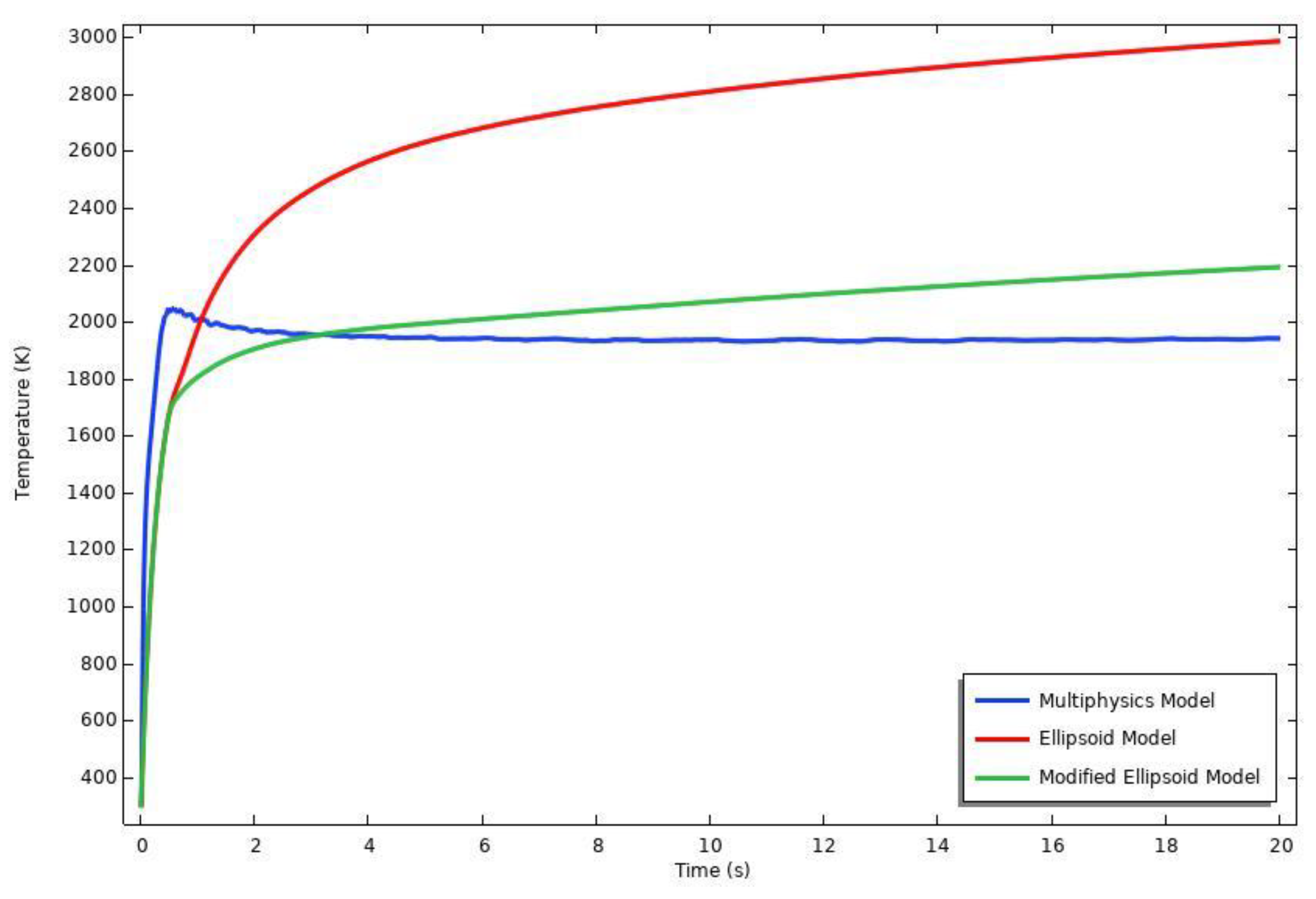
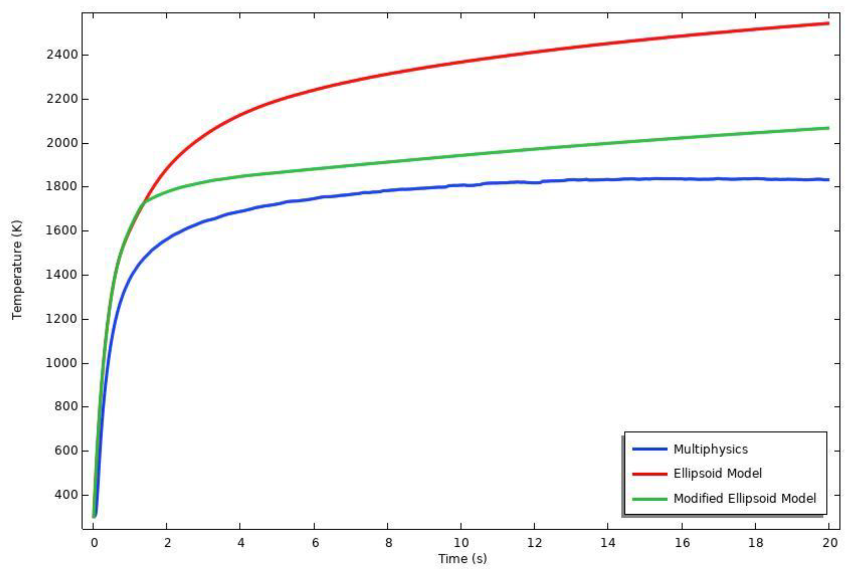
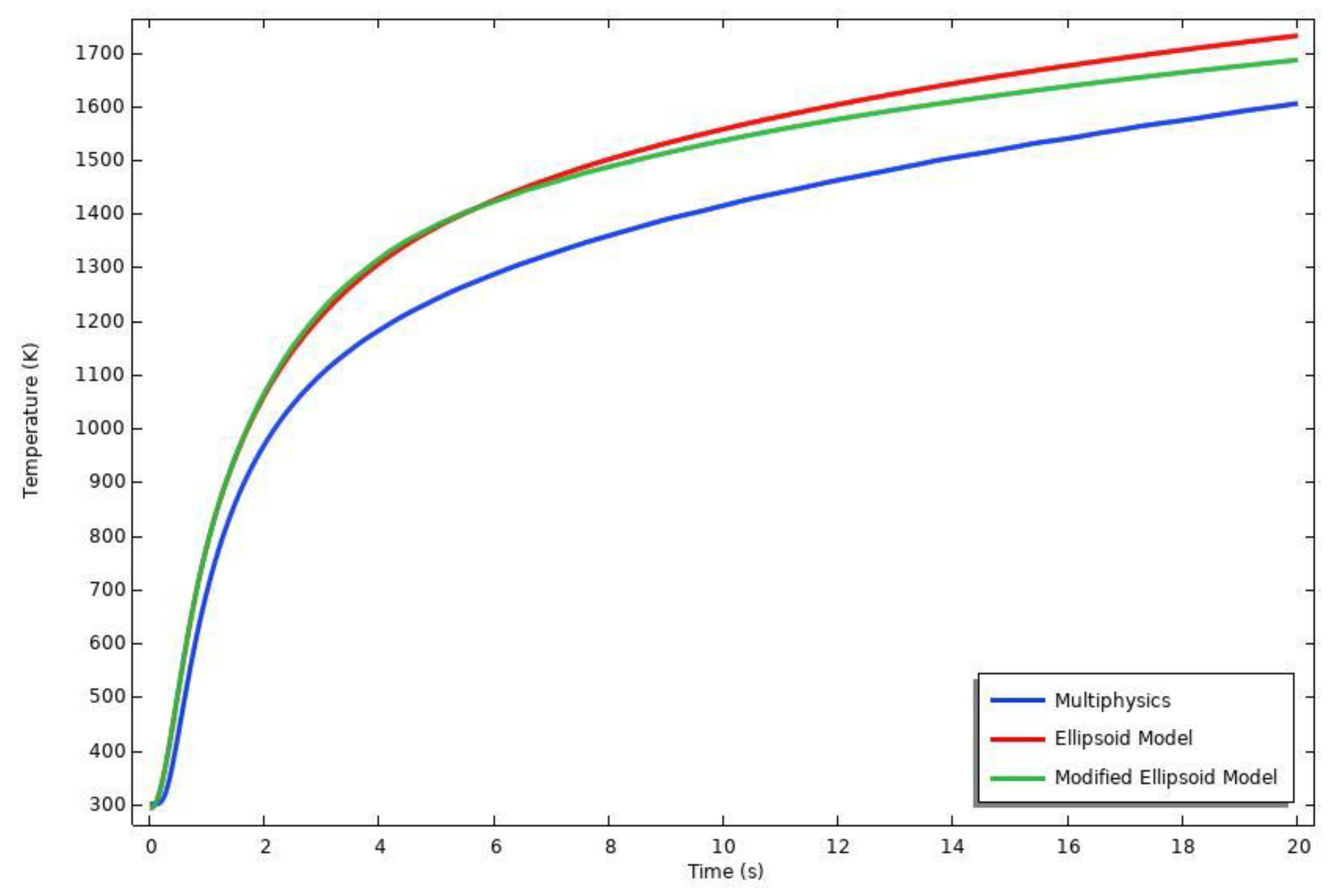
5.3. Comparison of Multiphysics, Convensional, and Modified Ellipsoid Models

After a multiphysics TIG welding model in the Comsol environment is developed and a specific TIG welding analysis is performed to obtain all necessary physical information in a welding pool, it is essential to find out the similarities and differences between Multiphysics and approximate models. In literature, it is well known that double-ellipsoidal heat source model (classical and modified forms) is a practical approach and easy to use for the finite element Method. [5,6,7,8]
Therefore, double-ellipsoid model is extensively studied for temperature distribution during the arc welding process in engineering applications.
Nart et al. [8] show that the accuracy of finite element welding simulations using double-ellipsoid approximate heat source model can be improved by increasing conductivity in 2D. It is true not only for particular nodes that are exceeding the melting temperature as suggested in reference [8], but also for all nodes in the welding pool region when the torch reaches the right-observation point to simulate the convective stirring effect (Modified double-ellipsoid method) in the welding pool. By doing so, irregular weld bead shapes can be analyzed by using double-ellipsoid heat source model without any difficulty.
Although the modification of double-ellipsoid heat source application in 2D works as shown in Reference [8], this intuitive approach needs to be verified using Multiphysics modeling in the Comsol environment. To do that, a new model in the COMSOL software environment as shown in Figure 17 is prepared for an approximated ellipsoidal heat source using the same welding parameters, geometry, and boundaries as used in the Comsol Multiphysics model. Additionally, Figure 18, Figure 19 and Figure 20 show the multiphysics, conventional and modified ellipsoidal model solutions for weld pool formation. Blue, red and green curves in figures shows the borders between FZ and HAZ.
Therefore, for comparing the results of these different welding models, for each model, five different locations are selected and defined as shown in Figure 17.
Four of them are located inside the weld pool region. Additionally, the last one is selected to be in heat affected zone. If the temperature histories of all corresponding points are compared, good results are obtained. Especially, for observation locations at points 1 and 2, the application of the modified double-ellipsoid method significantly generates closer temperature history than that of conventional ellipsoidal method as shown in Figure 21 and 22.
Particularly, this situation is very important in the middle part of the fusion zone. A good approximation of temperature history in this region affects the acceptable residual stress calculations. Moreover, this improved accuracy in predictions at the low cost of computer power and opens a new way for more reliable simulations of welding in various welding problems such as hot cracking that takes place in fusion zone (FZ) at high temperatures.
Similarly, at point 3 in the heat-effected zone (HAZ), the ellipsoidal methods give a similar temperature history until the metal melts as shown in Figure 23. However, after the melting, the modified ellipsoidal method gets closer to the multiphysics solution slowly. Furthermore, for point 4, both ellipsoidal methods give also similar temperature histories as shown in Figure 24. The modified ellipsoidal method gets closer to the multiphysics solution as time increases. Finally, in point 5, temperature histories between multiphysics and modified ellipsoidal methods develop good agreement. Corresponding the temperature differences get close to each other gradually as the stirring effect becomes dominant at the vertical direction in Figure 25.

6. Conclusions

In this research, an application of ellipsoidal heat source formulation is widely studied for obtaining better temperature distribution during arc welding for real-world applications. It is found that ellipsoidal approximate heat source model with artificially changing the coefficient of thermal conductivity in the welding pool area is a scientifically acceptable method by comparing the results of both approximated ellipsoidal heat source and the Comsol multi-physics arc welding model. Results show that temperature distributions obtained show a good approximation between multiphysics and modified application of ellipsoidal models concerning conventional usage of ellipsoidal model.
From all the results from all finite element analyses, it concluded that
  • The temperature distributions obtained show a good approximation between multiphysics and modified application of conventional models with respect to conventional usage of ellipsoidal model.
  • Especially in the middle of the pool region, the temperature history significantly changes and approaches to the multiphysics solutions.
  • Points inside and near the heat-effected zone in the pool region, both ellipsoidal methods give a similar temperature history until metal melts. After the melting occurs, the modified ellipsoidal method gets closer to the multiphysics solution slowly.
  • All implementations of the ellipsoidal method give similar temperature histories for points in the heat-effected zone.
Finally, the versatility of the modified ellipsoidal model provides a useful tool to get more accurate for industrial arc welding applications. Therefore, it can be stated that finite element modeling of the arc welding process using this approach estimates the corresponding residual stresses well enough for irregular bead cross-sections.

Acknowledgments

The authors express gratitude to the Scientific Research Projects Coordination Division (BAPK) at Sakarya University of Applied Science, for funding and support to this research.

References

  1. Udea, Y.; Yamakawa, T. Analysis of Thermal Elastic-Plastic Stress and Strain During Welding. Trans. Jpn. Weld. Soc. 1971, 2, 90–100. [Google Scholar]
  2. Chau, T.T.; Paradis, A.; Masson, J.C. A Simple Method for Evaluating the 3D Welding Effects on the Stiffened Panel Assemblies in Shipbuilding, 3th Int. Conf. on Marine Tech. III 1999, 485–530. [Google Scholar]
  3. Rosenthal, D. The Theory of Moving Sources of Heat and Its Application to Metal Treatments. Trans ASME, 1946, 68, 849–65. [Google Scholar] [CrossRef]
  4. Pavelic, V.; Tanbakuchi, R.; Uyehara, O.A; Myers, P.S. Experimental and Computed Temperature Histories in Gas Tungsten Arc Welding of Thin Plates, Weld J. Res Suppl. 1969, 48, 295–305. [Google Scholar]
  5. Goldak, J. ; Chakravarti, A; Bibby M. A New Finite Element Model for Welding Heat Sources. Metallurgical Transactions B 1984, 15, 299–305. [Google Scholar] [CrossRef]
  6. Kollár, D. Numerical Modelling on the Influence of Repair Welding During Manufacturing on Residual Stresses and Distortions of T-Joints. Results in Eng. 2023, 20. [Google Scholar] [CrossRef]
  7. Obeid, O.; Anthony, J.L; Olabi, A.G. Influence of Girth Welding Material on Thermal and Residual Stress Fields in Welded Lined Pipes. International Journal of Pressure Vessels and Piping 2022. [CrossRef]
  8. Nart, E.; Celik, Y. A Practical Approach for Simulating Submerged Arc Welding Process Using FE Method. Journal of Const. Steel Research 2013, 84, 62–71. [Google Scholar] [CrossRef]
  9. Wu, C.S.; Ushio, M.; Tanaka, M. Analysis of the TIG Welding Arc Behavior. Computational Materials Science 1997, 308–314. [Google Scholar] [CrossRef]
  10. Hsu, K.C.; Etemadi, K.; Pfender, E. Study of the Free-Burning High-Intensity Argon Arc. Journal of Applied Physics 1983, 54, 1293. [Google Scholar] [CrossRef]
  11. Tanaka, M.; Lowke, J.J. An Introduction to Physical Phenomena in Arc Welding Processes. Welding International 2004, 18, 11. [Google Scholar] [CrossRef]
  12. Tanaka, M.; Lowke, J.J. Predictions of weld pool profiles using plasma physics. Journal of Physics D-Applied Physics 2007, 40, R1–R23. [Google Scholar] [CrossRef]
  13. Tredia, A. Multiphysics Modeling and Numerical Simulation of GTA Weld Pools, Ph.D. Dissertation in Ecole Polytechnique 2011, France. [Google Scholar]
  14. Yan, L. S. ; C., Wang, L.; Chuansong, W. An Easy-To-Use Multi-Physical Model to Predict Weld Pool Geometry in Keyhole Plasma Arc Welding. Results in Engineering 2022, 14. [Google Scholar] [CrossRef]
  15. Sahoo, P.; Debroy, T.; McNallan, M.T. , Surface Tension of Binary Metal Surface Active Solute Systems Under Conditions Relevant to Welding Metallurgy. Metallurgical Transactions B 1988, 19B, 483–491. [Google Scholar] [CrossRef]
  16. Ushio, M. and Wu, C.S. Mathematical Modeling of Three-Dimensional Heat and Fluid Flow in a Moving Gas Metal Arc Weld Pool. Metallurgical and Materials Transactions B-Process Metallurgy and Materials Processing Science 1997, 28, 509–516. [Google Scholar] [CrossRef]
  17. Lowke, J.J. A Unified Theory of Arcs and their Electrodes. Le Journal de Physique IV, France 1997, 7, C4-283–C4-294. [Google Scholar] [CrossRef]
  18. COMSOL Plasma Module User’s Guide, pp. 324, www.comsol.com.
  19. Mishra, S. , Lienert, T. J., Johnson, M.Q. and Debroy, T. An Experimental and Theoretical Study of Gas Tungsten Arc Welding of Stainless Steel Plates with Different Sulfur Concentrations. Acta Materialia 2008, 56, 2133–2146. [Google Scholar] [CrossRef]
  20. Brent, D. , Voller, V.R. and Reid, K.J. Enthalpy-Porosity Technique for Modeling Convection-Diffusion Phase Change : Application to the Melting of Pure metal. Numerical Heat Transfer 1988, 13, 297–318. [Google Scholar] [CrossRef]
  21. Tanaka, M. , Terasaki, H., Ushio, M. and Lowke, J.J. Numerical Study of a Free-Burning Argon Arc with Anode Melting, Plasma Chemistry and Plasma Processing 2003, 23. [CrossRef]
  22. J.J. Lowke.. Simple theory of free-burning arcs. Journal of Physics D: Applied Physics 1979, 12, 1873. [CrossRef]
Figure 1. Finite Element Model and its dimensions (mm).
Preprints 151388 g001
Figure 2. Some physical properties of workpiece (anode, 304 SS material).
Preprints 151388 g002
Figure 3. Some physical properties of the workpiece (304 SS material) and shield gas (Argon).
Preprints 151388 g003
Figure 4. Some physical properties of shield gas (Argon).
Preprints 151388 g004
Figure 5. Flowchart for Multiphysics, conventional, and modified ellipsoid model procedures.
Preprints 151388 g005
Figure 6. 200 A, 10 mm arc length, argon arc axial temperature distribution, and a comparison with the literature [17].
Preprints 151388 g006
Figure 7. 200 A, 10 mm arc length, argon arc axial temperature distribution.
Preprints 151388 g007
Figure 8. 200 A, 10 mm arc length, argon arc axial pressure, and a comparison with the literature [17].
Preprints 151388 g008
Figure 9. 200 A, 10 mm arc length, argon arc axial velocities, and a comparison with [17].
Preprints 151388 g009
Figure 10. 200 A, 10 mm arc length, argon arc axial velocity distribution .
Preprints 151388 g010
Figure 11. Temperature distribution in weld pool region (150 A, 5 mm arc length).
Preprints 151388 g011
Figure 12. Temperature and velocity distribution in weld pool region in 3D (150 A, 20 s, 5 mm arc length).
Preprints 151388 g012
Figure 13. Temperature and velocity distribution in weld pool region in 3D (150 A, 20 s, 5 mm arc length).
Preprints 151388 g013
Figure 14. Temperature and velocity distribution in weld pool region (150 A, 20 s, 5 mm arc length).
Preprints 151388 g014
Figure 15. Zoom view of Temperature and velocity distribution in weld pool region (150 A, 20 s ,5 mm arc length).
Preprints 151388 g015
Figure 16. Experimental results (150 A, 20 s ,5 mm arc length).
Preprints 151388 g016
Figure 17. Model and Sampling points for comparing multiphysics and modified ellipsoidal models.
Preprints 151388 g017
Figure 18. Multiphysics weld pool region at 20s.
Preprints 151388 g018
Figure 19. Ellipsoidal weld pool regions at 20s.
Preprints 151388 g019
Figure 20. Modified Ellipsoidal weld pool regions at 20s.
Preprints 151388 g020
Figure 21. Temperature history for point 1.
Preprints 151388 g021
Figure 22. Temperature history for point 2
Preprints 151388 g022
Figure 23. Temperature history for point 3.
Preprints 151388 g023
Figure 24. Temperature history for point 4.
Preprints 151388 g024
Figure 25. Temperature history for point 5.
Preprints 151388 g025
Table 1. Material properties of workpiece metal (anode, 304 SS material).
Symbol Property Value/Unite
A γ Constant in surface tension gradient 4.3 e-4 N m-1 K-1
γ m o Surface tension of pure metal at the melting point 1.943 N m-1
T m Melting temperature of anode metal 1723 K
R g Gas constant 8314.3 J kg-1 mol-1 K-1
Γ s Surface access at saturation 1.3e-8 kg mol m-2
k 1 Constant related to the entropy of segregation 3.18e-3
Δ H o Standard heat of adsorption -1.662e8 J kg-1 mol-1
a i Activity of the surface active species ( wt pct sulfur) 0.022
Table 2. Physical Variable and Constants.
Symbol Description Dimension
z,r The axial, radial coordinate m
vr,vz Radial and axial velocity m s-1
t Time s
ρ Density kg m-3
p Pressure N m-2
pCF Arc pressure of the anode surface N m-2
μ Viscosity kg m-1 s-1
FVr,FVz Axial and radial volumetric forces N m-3
ρ0 Gas density in the arc plasma domain kg m-3
jr,jz Axial, radial current density A m-2
jCF Current density of the anode surface A m-2
j0 Welding current density A m-2
g Acceleration of gravity m s-2
Bθ Azimuthal magnetic flux density Wb m-2
Ar,Az Radial and axial Magnetic vector potential Wb m-2
μ0 Magnetic permeability of vacuum H m-1
φ Potential V
σ Electric conductivity S m-1
T Temperature K
cp Heat capacity J kg-1 K-1
k Thermal conductivity W m-1 K-1
Sv Volumetric heat source W m-3
q Heat flux density W m-2
qCF Heat flux density of the anode surface W m-2
E Electric field V m-1
kB Boltzmann's constant J K-1
Qrad Radiation loss W m-3
e Electronic charge C
FElectrode Additional energy flux of the cathode W m-2
FAnode Additional energy flux of the anode W m-2
ε The emissivity of the surface
α Stefan-Boltzmann constant W m-2 K-4
ϕK The work function of the cathode V
ϕA The work function of the anode V
ϕeff The effective work function of the cathode V
je Electron current density A m-2
ji Ion current density A m-2
jR Richardson-Dushman current density A m-2
Vi The ionization potential of the plasma V
AR Richarson’s constant A m-2K-2
β Thermal expansion coefficient of molten metal K-1
ρm Molten metal density in the weld pool kg m-3
dγ/dT Surface tension gradient N m-1 K-1
γ Surface tension coefficient N m-1
Aγ Constant in surface tension gradient N m-1 K-1
γ m 0 Surface tension of pure metal at the melting point N m-1
Tm Melting temperature of anode metal K
Rg Gas constant J kg-1 mol-1 K-1
Γs Surface access at saturation kg mol m-2
k1 Constant related to entropy of segregation
ΔH0 Standard heat of adsorption J kg-1 mol-1
ai Activity of the surface active species ( wt pct sulfur)
K Equilibrium constant for segregation
cpeq Equivalent specific heat for phase change J kg-1 K-1
Lf Latent heat for fusion J kg-1 K-1
fL Liquid fraction
Ts,TL Solidus and liquidus temperature of metal K
μL The viscosity of liquid metal kg m-1 s-1
μS Viscosity of solid metal kg m-1 s-1
Table 3. Boundary conditions for all studies.
Model Type Ssss
Sub-Dicipline
Boundary Conditions
Plasma Physics Model Electric
Currents
AD : Axial Symmetry ( φ r = 0), DE : Graund (φ = 0),
EF,FG,GI : Electric Insulation (n.J = 0), AI :Normal Current Density (−n.J = J0)
Magnetic
Fields
AD : Axial Symmetry B = 0, AG,GE,ED : Magnetic Insulation (n x A = 0)
Heat
Transfer
AD : Axial Symmetry ( T r = 0), DE,EF : Convective Heat Flux (q0 = h.(Text – T))
AG,GF : Temperature (T = 300 K), BKJI : Boundary Heat Source (Eq.11)
CF : Boundary Heat Source (Eq.15)
Fluid
Flow
AC : Axial Symmetry ( v z r = 0, vr = 0), CF, BKJI : Wall (vr = 0, vz = 0)
IH: inlet (vz = −Uargon), HG,GF : Open Boundary
MHD ( Magneto-Hydrodynamics)
Model
Electric
Currents
DC : Axial Symmetry ( φ r = 0), DE : Graund (φ = 0) , EF: Electric Insulation (n.J = 0)
CF : Normal Current Density obtained from the study 1 (−n.J = JCF)
Magnetic
Fields
CD : Axial Symmetry (B = 0), DE,EF,FC : Magnetic Insulation (n x A = 0)
Heat
Transfer
DC : Axial Symmetry ( T r = 0), DE,EF : Convective Heat Flux (q0 = h.(Text – T))
CF : Boundary Heat Source obtained from the study 1 (−n.q = qCF)
Fluid
Flow
DC : Axial Symmetry ( v z r = 0, vr = 0), DE,EF : Wall (vr = 0, vz = 0)
CF : Boundary stress obtained from the study 1 arc pressure (−n.p = pCF)
Ellipsoid Heat Source Model Heat
Transfer
DC : Axial Symmetry ( T r = 0), DE,EF : Convective Heat Flux (q0 = h.(Text – T))
CF : Radiation loss
Note: Ellipsoid Volumetric Heat Source was applied to the welding pool geometry
Table 4. Material properties of Tungsten Cathode.
Property Value/Unite
Coefficient of thermal expansion 4.5e-6 K-1
Density 19350 kg m-3
Heat capacity 132 J kg-1 K-1
Thermal conductivity 175 W m-1 K-1
Electrical conductivity 20e6 S/m
Table 5. Experimental weld pool dimensions and a comparison with the literature [21].
Depth/Half Width
Tanaka’s Experiment 4.30 m m / 5.09 m m
(Ref [21])
Preprints 151388 i001
Tanaka’s Results 4.91 m m / 5.48 m m
(Ref [21] )
Our Results 4.25 m m / 5.40 m m
Figure 15

Experiments
4.068mm / 4.40mm
Figure 16 (150 A, 20 s ,5 mm arc length)
Disclaimer/Publisher’s Note: The statements, opinions and data contained in all publications are solely those of the individual author(s) and contributor(s) and not of MDPI and/or the editor(s). MDPI and/or the editor(s) disclaim responsibility for any injury to people or property resulting from any ideas, methods, instructions or products referred to in the content.
Copyright: This open access article is published under a Creative Commons CC BY 4.0 license, which permit the free download, distribution, and reuse, provided that the author and preprint are cited in any reuse.
Prerpints.org logo

Preprints.org is a free preprint server supported by MDPI in Basel, Switzerland.

Subscribe

Disclaimer

Terms of Use

Privacy Policy

Privacy Settings

© 2025 MDPI (Basel, Switzerland) unless otherwise stated