Remote Sensing and Deep Learning Based Soil Moisture Monitoring System Using HCSWO Optimization Technique and AGRL-RBFN

1. Introduction

Soil moisture serves as a crucial factor in governing the interactions of water, energy, and carbon cycles between terrestrial ecosystems and the atmosphere. Consequently, data on soil moisture is vital for a range of environmental research areas, such as hydrology, climatology, meteorology, agriculture, water resource management, and the study of climate change. In agriculture, soil moisture data is crucial for assessing drought severity, determining the onset of the rainy season, scheduling planting activities, and providing early alerts regarding potential yield reductions. As climate conditions change, the significance and challenges associated with monitoring soil moisture will increase markedly. To ensure the healthy growth of plants, it is crucial to keep soil moisture levels within an ideal range, preventing both excessive saturation and drought. Soils that are too wet can cause the leaching of essential nutrients, whereas soils that are too dry may result in diminished crop yields and compromised quality. A lack of adequate moisture can lead to plant mortality and reduced crop yields, whereas an excess of moisture may cause root diseases (Pal & Bodhe, 2023). To address this concern, regular soil moisture monitoring is conducted. This monitoring frequently employs probe techniques to facilitate informed decision-making regarding irrigation practices, crop management, and water conservation initiatives. Accurate forecasting of soil moisture levels is vital for evaluating farmland quality (Abbes et al., 2024) (Yang et al., 2024). Remote sensing technology serves as a robust alternative for large-scale soil moisture monitoring, providing high spatial and temporal resolution. Currently, soil moisture data derived from remote sensing is supplied by the National Aeronautics and Space Administration (NASA) and the European Space Agency’s Soil Moisture and Ocean Salinity (SMOS) mission (Wang et al., 2023) (Lee et al., 2023). In recent years, machine learning and deep learning methodologies have been employed to estimate soil moisture from this data. The methodology is capable of automatically extracting significant features from raw data and adeptly managing complex relationships within large datasets (Li & Yan, 2024). Current research predominantly employs machine learning techniques such as Support Vector Machines (SVM), k-nearest neighbors (KNN) (Uthayakumar et al., 2022), Random Forest (RF), and Artificial Neural Networks (ANN), which enhance accuracy in soil moisture estimation (Liu et al., 2022, Shokati et al., 2024). These methods effectively capture intricate relationships and mitigate the risk of overfitting (Win et al., 2024) (Peng et al., 2024). Convolutional Neural Networks (CNN) are particularly adept at considering spatial arrangements, thereby facilitating the extraction of deeper features (Liu et al., 2021) (Hegazi et al., 2023). Long Short-Term Memory (LSTM) networks are utilized to effectively capture temporal dynamics and to create a virtual soil moisture sensor using data from other node transducers (Babu & Yadavamuthiah, 2024) (Patrizi et al., 2022).

Roberts et al. (2022) introduced a deep learning model aimed at estimating soil moisture through the use of remote sensing data. This model employs a Convolutional Neural Network (CNN) to process reflection measurements and surface parameters, thereby improving the accuracy of global soil moisture estimations. The analysis of results indicates that the CNN method outperforms existing models in terms of accuracy; however, the framework demonstrates limitations in areas characterized by minimal variation in soil moisture.

Singh et al. (2024) introduced a machine learning (ML) methodology for predicting soil moisture utilizing Wireless Sensor Networks (WSN). The study primarily employed Random Forest (RF), Support Vector Machines (SVM), and Long Short Term Memory (LSTM) techniques for monitoring soil moisture levels. The findings indicate that the LSTM model consistently surpasses other ML algorithms across various evaluation metrics; however, it necessitates greater computational resources and extended training durations, which may impact the overall performance of the research framework.

Dabboor et al. (2023) established a deep learning framework aimed at predicting soil moisture content from satellite data through the application of several optimized machine learning models. The Gaussian Process Regression (GPR) and Artificial Neural Network (ANN) methods were utilized in the prediction process. The results demonstrate that the GPR model excelled compared to other ML models in accurately estimating soil moisture content, achieving a root mean square error (RMSE) of 4.05%. Nonetheless, the training time is prolonged due to the extensive hyperparameter tuning involved.

Nijaguna et al. (2023) introduced a deep learning methodology for the retrieval of soil moisture from remote sensing imagery. They employed a Gated Recurrent Unit (GRU) hybrid classifier for determining soil moisture content. The findings suggest that this hybrid classifier outperforms other models in terms of performance. Nevertheless, the conventional feature selection method did not encompass all significant features that could influence the research outcomes.

Liu et al. (2023) proposed a machine learning technique for estimating soil moisture utilizing multi-source remote sensing images. The Extreme Trees (ETr) and Random Forest (RF) models were effectively implemented for this estimation. While the ETr model demonstrated superior predictive accuracy compared to other models, it encountered overfitting issues due to the lower spatial resolution of the satellite imagery.

Adab et al. (2020) introduced a machine learning model aimed at estimating surface soil moisture utilizing remote sensing data. The study employed Random Forest (RF), Support Vector Machine (SVM), and Artificial Neural Network (ANN) models to improve soil moisture predictions. The findings indicate that the RF method outperformed traditional models; however, it is constrained by limited spatial coverage and inadequate measurements, which complicate accurate estimations.

Celik et al. (2022) concentrated on predicting soil moisture from remote sensing images through a deep learning approach. The Long Short-Term Memory (LSTM) method was utilized for this prediction. The results of the experimental analysis demonstrate that the LSTM approach surpassed existing models; nevertheless, inaccuracies were observed due to variations in soil texture data derived from the remote sensing images.

However, existing studies do not adequately address the complexities involved in predicting soil moisture in the context of climatic changes, and they lack comprehensive background information. Specifically, current research studies exhibit several limitations, which are outlined as follows:

• Climate change significantly influences soil moisture patterns through variations in temperature and extreme weather events. To date, there is little research focused on the complexity of predicting soil moisture in the context of changing climate conditions.

• Remote sensing data may be compromised by noise or other atmospheric influences. Many existing methodologies have overlooked this issue, complicating the development of accurate models.

• Gaps in remote sensing data often arise due to cloud cover, sensor malfunctions, and other factors. This results in incomplete soil moisture information, which has not been adequately addressed in current methodologies.

• Soil moisture dynamics occur across various spatial and temporal scales, and existing models are unable to encapsulate all relevant information within a single framework.

This study proposes an AGRL-RBFN approach for the soil moisture prediction process. The research methodology applied delineates specific objectives designed to tackle the identified research problems:

• To forecast soil moisture trends in relation to climatic changes through the application of the AdaK-MCC approach.

• To create precise models for soil moisture prediction by eliminating the influence of extraneous factors using the SGF approach.

• To predict soil moisture utilizing comprehensive data sets that are devoid of any gaps, employing the AdaK-MCC approach.

• To consolidate all relevant information pertaining to soil moisture prediction into a singular model by leveraging the FWFCSD approach.

The organization of the research paper is delineated as follows: Section 2 details the proposed methodology. In Section 3, the effectiveness of the proposed methodology is evaluated in comparison to existing studies. Finally, Section 4 concludes the paper and discusses potential future improvements.

2. Materials and Methods: Soil Moisture Prediction Using AGRL-RBFN with IL

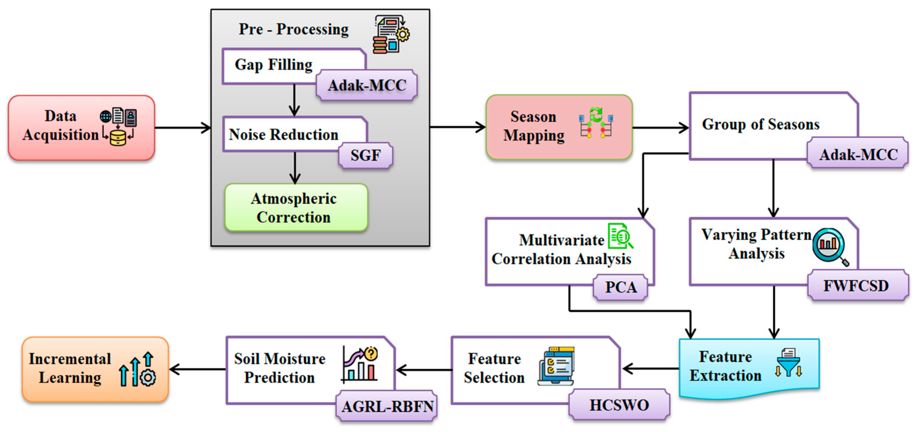
In the proposed study, soil moisture is forecasted utilizing remote sensing data through the AGRL-RBFN with an IL approach, while also monitoring climatic variations via seasonal mapping and categorization. The primary stages of the research include pre-processing, seasonal mapping and categorization, analysis of varying patterns and multivariate correlations, feature extraction and selection, culminating in the prediction of soil moisture. The structural diagram representing the proposed soil moisture prediction methodology is depicted in Figure 1.

2.1. Data Acquisition

The procedure for monitoring soil moisture utilizing remote sensing and deep learning commences with the collection of remote sensing data related to soil moisture. These sensors are capable of assessing soil moisture across extensive regions without requiring direct physical sampling. The gathered remote sensing data (Z) on soil moisture is represented as follows:

$${\rm Z}=\left\{{{\rm Z}}^1,{{\rm Z}}^2,{{\rm Z}}^3,\mathrm{........}{{\rm Z}}^a\right\}$$

(1)

Where,$\left(a\right)$ illustrates total number of $\left({\rm Z}\right)$. This continuous and spatially extensive data collection significantly enhances the accuracy of soil moisture predictions.

2.2. Pre-Processing

In this pre-processing phase, $\left({\rm Z}\right)$ is pre-processed to ensure more accurate and reliable soil moisture predictions from the remote sensing data.

2.2.1. Gap Filling

The missing values in $\left({\rm Z}\right)$ are filled using the AdaK-MCC method. By grouping similar observations, K-Means Clustering (KMC) identifies patterns within the data, enabling more accurate imputations for missing values and ensuring their contextual relevance. However, the final clusters can be significantly influenced by the initial placement of centroids. Poor initialization may lead to suboptimal clustering, which can affect the accuracy of the imputed values. To address this, Adaptive Momentum Coefficients (AMCs) is used for centroid initialization, allowing centroids to explore the solution space more effectively and enhancing the imputation of missing data. Firstly, clusters $\left(\beta \right)$ are selected from $\left({\rm Z}\right)$, and the centroids $\left({\varsigma }^j\right)$ are initialized using AMC, where centroids can explore the solution space more widely, reducing the risk of local minima. $\left({\varsigma }^j\right)$ is initialized as:

$${\varsigma }^j=\vartheta •{\varsigma }^{j-1}+\left(1-\vartheta \right)\ast \sout{\nabla }\sout{G}$$

(2)

$$\sout{\nabla }\sout{G}=-{\displaystyle \frac{1}{a}}{\displaystyle \sum _{i=1}^a{\displaystyle \sum _{j=1}^{\beta }\left(h^{ij}•\left({{\rm Z}}^i,{\varsigma }^j\right)\right)}}$$

(3)

Where, $\left({\varsigma }^j\right)$ and $\left({\varsigma }^{j-1}\right)$ indicates the current and previous centroid, $\left(\vartheta \right)$ represents the momentum coefficient of centroid, $\left(h^{ij}\right)$ specifies the distance between $\left(i^{th}\right)$ input $\left({\rm Z}\right)$ and $\left(j^{th}\right)$ centroid $\left({\varsigma }^j\right)$, $\left(\sout{\nabla }\sout{G}\right)$ refers to the gradient loss function. Next, each data point is assigned to the nearest centroid based on the distance as given by:

$${{\rho }^{″}}_i=\arg \underset{j}{\min } \left({‖\left({{\rm Z}}^i-{\varsigma }^j\right)‖}^2\right)$$

(4)

Here, $\left({{\rho }^{″}}_i\right)$ denotes cluster assigned to data $\left({{\rm Z}}^i\right)$ and $\arg \underset{j}{\min }$ refers to the minimum argument in the $\left(j^{th}\right)$ cluster. The centroids are recalculated based on the data point that is already assigned to the cluster. The updated centroid $\left({{\varsigma }^{\prime }}^j\right)$ is:

$${{\varsigma }^{\prime }}^j={\displaystyle \frac{1}{\left|\left.{{\rho }^{″}}_i\right|\right.}}{\displaystyle \sum _{{{\rm Z}}^i\in {{\rho }^{″}}_i}{{\rm Z}}^i}$$

(5)

Where, $\left|\left.{{\rho }^{″}}_i\right|\right.$ is the number of data points in cluster $\left({\varsigma }^j\right)$. By summing this, updated centroid is produced. The above steps are repeated until the maximum number of iterations $\left({\stackrel{⃛}{t}}_{\max }\right)$ is reached. Once the final clusters are formed, the missing values are imputed based on the values of similar points in the same cluster and are denoted as $\left(D_{gfill}\right)$. The pseudocode for AdaK-MCC is expressed below.

Pseudo code of AdaK-MCC Input: Soil Moisture Data $\left({\rm Z}\right)$ Output: Gaps Filled Data $\left(D_{gfill}\right)$ Begin     Initialize $\left(\beta \right)$, $\left({\varsigma }^j\right)$, minimum iteration $\left({\stackrel{⃛}{t}}_{\min }\right)$, maximum iteration $\left({\stackrel{⃛}{t}}_{\max }\right)$     While $\left({\stackrel{⃛}{t}}_{\min }<{\stackrel{⃛}{t}}_{\max }\right)$         Derive $\left({\varsigma }^j\right)$ # using Adaptive Momentum Coefficients                 ${\varsigma }^j=\vartheta •{\varsigma }^{j-1}+\left(1-\vartheta \right)\ast \sout{\nabla }{\sout{G}}^o$         Assign $\left({{\rho }^{″}}_i\right)$ to data $\left({{\rm Z}}^i\right)$                 ${{\rho }^{″}}_i=\arg \underset{j}{\min } \left({‖\left({{\rm Z}}^i-{\varsigma }^j\right)‖}^2\right)$         Update centroid $\left({\varsigma }^j\right)$                 ${{\varsigma }^{\prime }}_j={\displaystyle \frac{1}{\left|\left.{{\rho }^{″}}_i\right|\right.}}{\displaystyle \sum _{{{\rm Z}}^i\in {{\rho }^{″}}_i}{{\rm Z}}^i}$         Repeat until $\left({\stackrel{⃛}{t}}_{\max }\right)$     End while     Return $\to \left(D_{gfill}\right)$ End

Therefore, the gaps in the soil moisture data are filled, leading to improved accuracy in the models used for soil moisture estimation.

2.2.2. Noise Reduction

The noises in the gaps filled data $\left(D_{gfill}\right)$ are reduced by using SGF. It is a smoothing filter that effectively reduces noise while preserving critical features in soil moisture data, making it especially useful for analyzing spectral data related to soil moisture content. The noise reduced data $\left({{\rm N}}_{nred}\right)$ is determined as,

$${{\rm N}}_{nred}={\displaystyle \sum _{u=\frac{1-d}{2}}^{\frac{d-1}{2}}{J}_u\ast D_{gfill v+u}}$$

(6)

Where, $\left(J_u\right)$ refers to filter coefficient for each index $\left(u\right)$, $\left(d\right)$ indicates the length of the moving window, and $\left(D_{gfill v+u}\right)$ represents input at index $\left(v+u\right)$ within the window.

2.2.3. Atmospheric Correction

Here, the atmospheric noises present in the noise reduced data $\left({{\rm N}}_{nred}\right)$ are corrected.

Atmospheric noise pertains to undesirable interferences that may compromise the precision of remote sensing measurements, frequently resulting from phenomena such as lightning, thunderstorms, and other natural disturbances.

The atmospheric noise refers to unwanted disturbances that can affect the accuracy of remote sensing measurements, often caused by factors like lightning, thunderstorms, and natural disturbances. The data, after correction for atmospheric noise, $\left(C_{atno}\right)$ is expressed as follows:

$$C_{atno}=f\left({{\rm N}}_{nred}\right)$$

(7)

Where, $\left(f\right)$ denotes the noise correction function. The purpose of this correction is to remove atmospheric noises, ensuring that the measurements accurately reflect the true moisture content of the soil. The final pre-processed data is specified as $\left(\ddot{\Re }\right)$.

2.3. Season Mapping

After pre-processing the data, climatic seasons are mapped based on the date, year, and month to distinguish soil moisture patterns influenced by climatic variations. The four seasons spring $\left(S_{spr}\right)$, summer $\left(S_{sum}\right)$, autumn (fall) $\left(S_{aut}\right)$, and winter $\left(S_{win}\right)$ are mapped. The mapped seasons $\left({\Phi }^{sea}\right)$ are expressed as follows:

$${\Phi }^{sea}=\left\{\begin{array}{l}{S}_{spr}, if m \left(\delta , \gamma \right)\in \left\{3,4,5\right\} \\ S_{sum}, if m \left(\delta , \gamma \right)\in \left\{6,7,8\right\}\\ S_{aut}, if m \left(\delta , \gamma \right)\in \left\{9,10,11\right\}\\ S_{win}, if m \left(\delta , \gamma \right)\in \left\{12,1,2\right\}\end{array}\right.$$

(8)

Where, $m \left(\delta , \gamma \right)$ represents the month along with the date and year in the dataset $\left(\ddot{\Re }\right)$, while the numbers $\left\{1,2,\mathrm{....12}\right\}$ correspond to the 12 months of the year from January to December. This seasonal mapping facilitates a clearer comprehension of the variations in soil moisture levels across different seasons.

2.4. Group of Seasons

In this phase, based on the mapped seasons $\left({\Phi }^{sea}\right)$, the data are grouped using AdaK-MCC. KMC has the capability to categorize soil moisture data according to comparable seasonal traits, thereby facilitating the analysis of moisture fluctuations throughout various seasons such as spring, summer, autumn, and winter. The resulting clusters may be affected by inadequate centroid initialization; therefore, AMC is employed for this purpose, which aids in preventing local minima and improving the seasonal classification. The AdaK-MCC method is detailed in section 3.2.1. The grouped seasons are determined as $\left(G_{season}\right)$.

2.5. Varying Pattern Analysis

Now, the variability patterns in the grouped seasons $\left(G_{season}\right)$ are analyzed using FWFCSD, as soil moisture data exhibit seasonal patterns affected by climatic variations. Fourier Series Decomposition (FSD) breaks the data into frequency components, helps to analyze both short-term fluctuations and long-term trends. FSD assumes data continuity, but abrupt changes can distort Fourier coefficients. To address this, Frequency Weighted Fourier Coefficients (FWFC) are used to adjust the importance of coefficients based on each frequency, enabling more flexible analysis that adapts to changing soil moisture patterns over time. Firstly, the time series data in $\left(G_{season}\right)$ are decomposed into frequency components to analyze periodic patterns as follows:

$$\stackrel{⃛}{\sout{\chi }}\left(t\right)={\displaystyle \frac{{\eta }_0}{2}}+{\displaystyle \sum _{p=1}^{\infty }\left({\eta }_p \cos \left(p t\right)+{\stackrel{⃛}{\eta }}_p \sin \left(p t\right)\right)}$$

(9)

Where, $\stackrel{⃛}{\sout{\chi }}\left(t\right)$ represents frequency components in $\left(G_{season}\right)$ at time $\left(t\right)$, $\left({\eta }_0\right)$ indicates average soil moisture value, $\left({\eta }_p\right)$ and $\left({\stackrel{⃛}{\eta }}_p\right)$ are the Fourier coefficients of cosine and sine terms, $\left(p\right)$ denotes the index of $\left(G_{season}\right)$. In this context, the FWFC is employed in Fourier coefficients to facilitate a flexible analysis of varying conditions, serving as the weighting function associated with frequency $\left(\omega \left(F\right)\right)$and is expressed as follows:

$${\eta }_0={\displaystyle \frac{1}{\pi }}{\int }_{-\pi }^{\pi }\stackrel{⃛}{\sout{\chi }}\left(t\right) dt$$

(10)

$${\eta }_p=\omega \left(F\right)\ast {\displaystyle \frac{1}{\pi }}{\int }_{-\pi }^{\pi }\stackrel{⃛}{\sout{\chi }}\left(t\right) \cos pt dt$$

(11)

$${\stackrel{⃛}{\eta }}_p=\omega \left(F\right)\ast {\displaystyle \frac{1}{\pi }}{\int }_{-\pi }^{\pi }\stackrel{⃛}{\sout{\chi }}\left(t\right) \sin pt dt$$

(12)

Here, $\left(\pi \right)$ denotes the normalization factor. The analyzed variability pattern data $\left({\Psi }_{vapa}\right)$ is obtained, representing the varying soil moisture patterns.

2.6. Multivariate Correlation Analysis

In this phase, the multivariate correlations are analyzed for the grouped seasons $\left(G_{season}\right)$ using PCA. PCA helps to find patterns and relationships among variables by transforming correlated variables into uncorrelated principal components, thereby simplifying the understanding of the underlying data structure. The PCA steps are explained below.

Step 1: The first step is to standardize the data $\left(G_{season}\right)$, to ensure all variables are on the same scale. The standardized data $\left(\mathrm{A}\right)$ is given by:

$$\mathrm{A}={\displaystyle \frac{\left(G_{season}-\mu \right)}{\sigma }}$$

(13)

Where, $\left(\mu \right)$ and $\left(\sigma \right)$ are the mean and standard deviation of $\left(G_{season}\right)$, respectively.

Step 2: Next, the covariance matrix is computed to identify how the soil moisture variables vary with each other. The construction of covariance matrix is formulated as,

$$\mathrm{B}={\displaystyle \frac{1}{g}}\ast \left(\mathrm{A}\right){\left(\mathrm{A}\right)}^{\mathrm{T}}$$

(14)

Where, $\left(g\right)$ defines the total number of samples in $\left(G_{season}\right)$ and ${\left(\mathrm{A}\right)}^{\mathrm{T}}$depicts matrix transpose.

Step 3: Then, eigenvalues $\left({\mathrm{E}}_{value}\right)$ and eigenvectors $\left({\mathrm{E}}_{vector}\right)$ are computed to find the principal components that account for the greatest variance in the data as indicated by:

$$\mathrm{B}\ast {\mathrm{E}}_{vector}={\mathrm{E}}_{value}\ast {\mathrm{E}}_{vector}$$

(15)

The principal components $\left(\chi \right)$ are selected from $\left({\mathrm{E}}_{vector}\right)$, corresponding to the highest $\left({\mathrm{E}}_{value}\right)$. It is calculated as follows:

$$\chi =\mathrm{A}\ast {\mathrm{E}}_{vector}$$

(16)

From the obtained principal components $\left(\chi \right)$, the multivariate correlation analyzed data is obtained, and it is denoted as $\left({\Phi }_{muco}\right)$.

2.7. Feature Extraction

Here, features are extracted from both the varying pattern and multivariate correlation analyzed data $\left({\Psi }_{vapa}\right)$ and $\left({\Phi }_{muco}\right)$, to enhance the model's performance by simplifying complex data and improving predictions for soil moisture estimation. The extracted features $\left(\mathrm{Y}\right)$ are represented as:

$$\mathrm{Y}=〈{\mathrm{Y}}_1,{\mathrm{Y}}_2,{\mathrm{Y}}_3,\mathrm{.......}{\mathrm{Y}}_b〉$$

(17)

Here, $\left(b\right)$ indicates the total number of features extracted from both $\left({\Psi }_{vapa}\right)$ and $\left({\Phi }_{muco}\right)$, respectively. The features such as mean reflectance, standard deviation, peak positions, Normalized Difference Vegetation Index (NDVI), Soil Moisture Index (SMI), ratio indices, contrast, homogeneity¸ entropy, curvature metrics, inflection points, wavelet coefficients, energy of coefficients, reflectance ratios, derivative spectra are extracted from $\left({\Psi }_{vapa}\right)$. Then, from $\left({\Phi }_{muco}\right)$, features such as pairwise correlation coefficients, correlation heatmap, clustered correlation groups, representative bands, canonical variate, canonical correlation coefficients, regression weights, standardized coefficients¸ higher-order terms, unique contribution scores are extracted.

2.8. Feature Selection

From the extracted features $\left(\mathrm{Y}\right)$, the optimal features are selected using HCSWO. The Spider Wasp Optimizer (SWO) enhances soil moisture estimation by selecting high-quality feature subsets. However, SWO struggles with highly correlated features, leading to redundancy in selected features and potentially reducing the model’s performance. Therefore, a Hierarchical Correlation Matrix (HCM) is used to cluster correlated features, enabling SWO to focus on representative features from each cluster. This approach enhances model’s performance by ensuring selected features contribute uniquely to the predictive model. The steps of HCSWO are as follows.

Hierarchical Correlation Matrix

The correlation between each pair of extracted features $\left(\mathrm{Y}\right)$ is determined to cluster the correlated features. The correlation coefficient $\left({\perp }^{cor}\right)$ is defined as follows:

$${\perp }^{cor}={\displaystyle \frac{Cov\left({\mathrm{Y}}_b,{\mathrm{Y}}_{b+1}\right)}{\stackrel{⃛}{\sigma }\left({\mathrm{Y}}_b\right) \stackrel{⃛}{\sigma }\left({\mathrm{Y}}_{b+1}\right)}}$$

(18)

Here, $Cov\left({\mathrm{Y}}_b,{\mathrm{Y}}_{b+1}\right)$ denotes covariance between features $\left({\mathrm{Y}}_b\right)$ and $\left({\mathrm{Y}}_{b+1}\right)$ of $\left(\mathrm{Y}\right)$, $\stackrel{⃛}{\sigma }\left({\mathrm{Y}}_b\right)$and $\stackrel{⃛}{\sigma }\left({\mathrm{Y}}_{b+1}\right)$ refers to standard deviation between variables $\left({\mathrm{Y}}_b\right)$ and $\left({\mathrm{Y}}_{b+1}\right)$ of $\left(\mathrm{Y}\right)$. Next, to group the correlated features, hierarchical clustering on the correlation matrix $\left({\perp }^{cor}\right)$ is performed as follows:

$${\Delta }_{hier}=1-{\perp }_{cor}$$

(19)

Where, ${\Delta }_{hier}$ indicates the output of HCM, which shows the clusters of the correlated feature. From this, the representative features are represented as $\left({\mathrm{Y}}^{rep}\right)$.

Initialization:

Initially, the population of spider wasps $\left(\tilde{\Lambda }\right)$ is initialized within the search space concerning $\left({\mathrm{Y}}^{rep}\right)$ as follows:

$${\tilde{\Lambda }}_{m\times \mathcal{l}}={\left[\begin{array}{cccc}{\mathrm{Y}}^{rep}\left(1,1\right)& {\mathrm{Y}}^{rep}\left(1,2\right)& \cdots & {\mathrm{Y}}^{rep}\left(1,\mathcal{l}\right)\\ {\mathrm{Y}}^{rep}\left(2,1\right)& {\mathrm{Y}}^{rep}\left(2,2\right)& \cdots & {\mathrm{Y}}^{rep}\left(2,\mathcal{l}\right)\\ ⋮& ⋮& \cdots & ⋮\\ {\mathrm{Y}}^{rep}\left(m,1\right)& {\mathrm{Y}}^{rep}\left(m,2\right)& \cdots & {\mathrm{Y}}^{rep}\left(m,\mathcal{l}\right)\end{array}\right]}_{m\times \mathcal{l}}$$

(20)

$${\tilde{\Lambda }}_x=\left(u{b}_x-l{b}_x\right)\ast \xi +l{b}_x$$

(21)

Here, $\left(m\right)$ refers to the number of spider wasps (female) and $\left(\mathcal{l}\right)$ is the dimension of the search space. Then, the random position $\left({\tilde{\Lambda }}_x\right)$ of the spider wasp with $\left(\xi \right)$ random variable and $\left(u{b}_x,l{b}_x\right)$ the upper and lower bound of the $\left(x^{th}\right)$ spider wasp are expressed.

Fitness Evaluation

Next, the fitness value $\left({\Theta }_{fit}\right)$ that determines the optimal feature based on the classification accuracy $\left(\varpi \right)$ is determined as follows:

$${\Theta }_{fit}=\max \left[\varpi \right]$$

(22)

By using $\left({\Theta }_{fit}\right)$, the prey, which is the best feature, is selected and compared from the population during the mating stage.

Searching Phase

In this exploration phase, the female wasp searches the spiders to feed their young. The updated position $\left({\tilde{\Lambda }}_{x+1}\right)$ of the female wasp in the search phase is calculated as:

$${\tilde{\Lambda }}_{x+1}=\left\{\begin{array}{l}{\tilde{\Lambda }}_x+{\ddot{\mu }}_1\ast \left({{\tilde{\Lambda }}_x}^v-{{\tilde{\Lambda }}_x}^w\right), if q_3<q_4\\ {{\tilde{\Lambda }}_x}^{\stackrel{⃛}{w}}+{\ddot{\mu }}_2\ast \left(l{b}_x+q_2\ast \left(u{b}_x-l{b}_x\right)\right), Otherwise\end{array}\right.$$

(23)

Where, $\left({\ddot{\mu }}_1\right)$ and $\left({\ddot{\mu }}_2\right)$ denotes the constant motion, $\left(q_1,q_2,q_3,q_4\right)$ are random numbers, and $\left(v,w,\stackrel{⃛}{w}\right)$ indicates the index randomly selected from the population.

Following and Escaping Stage

This is the exploration and exploitation phase, here, after the prey (spider) is found, the wasp starts chasing the prey. The updated position is expressed as:

$${\tilde{\Lambda }}_{x+1}=\left\{\begin{array}{l}{\tilde{\Lambda }}_x+\cancel{\stackrel{⌢}{C}}\ast \left|2\ast q_5\ast \right|{{\tilde{\Lambda }}_x}^v-{\tilde{\Lambda }}_x, if q_3<q_4\\ {\tilde{\Lambda }}_x\ast \overrightarrow{ƛ}, Otherwise\end{array}\right.$$

(24)

The transition between searching, and following and escaping phase is given by:

$${\tilde{\Lambda }}_{x+1}=\left\{\begin{array}{l}equation \left(19\right)\text{}, if q_6<\kappa \\ equation \left(20\right),Otherwise\end{array}\right.$$

(25)

Here, $\left(\kappa \right)$ indicates control parameter, $\left(q_5,q_6\right)$ are random numbers, $\left(\cancel{\stackrel{⌢}{C}}\right)$ denotes distance controlling factor, and $\overrightarrow{ƛ}$ denotes a vector.

Hunting and Nesting Behavior

In this stage, the paralyzed spider is pulled into the pre-prepared nest. The final updated position in the hunting and nesting behavior stage is expressed as:

$${\tilde{\Lambda }}_{x+1}=\left\{\begin{array}{l}{\tilde{\Lambda }}_x^{\ast }+\cos \left(2\ddot{\pi }\dot{l}\right)\ast \left({\tilde{\Lambda }}_x^{\ast }-{\tilde{\Lambda }}_x\right), \text{} \text{}if q_3<q_4\\ {{\tilde{\Lambda }}_x}^v+q_3\ast \ddot{\gamma }\ast \left({{\tilde{\Lambda }}_x}^v-{\tilde{\Lambda }}_x\right)+\left(1-q_3\right)\ast \dot{\stackrel{\rightharpoonup }{R}}\ast \left({{\tilde{\Lambda }}_x}^w-{\tilde{\Lambda }}_x^{\stackrel{⃛}{w}}\right), otherwise\end{array}\right.$$

(26)

Where, $\left({\tilde{\Lambda }}_x^{\ast }\right)$ indicates best available solution, $\left(\ddot{\pi }\right)$ is a constant, $\left(\ddot{\gamma }\right)$ represents a number generated based on Levy flight, $\left(\dot{l}\right)$ indicates the localization factor, and $\left(\dot{\stackrel{\rightharpoonup }{R}}\right)$ signifies the binary vector.

Mating Behavior

The mating behavior is the last stage, and it seeks to determine the offspring’s locations and enhance their positions. A new offspring is produced by performing crossover between selected male and female wasps. Next, based on the fitness value $\left({\Theta }_{fit}\right)$, the new offspring replaces current population members. The position the population is updated by selecting the spider wasps with the best fitness values $\left({\Theta }_{fit}\right)$. By iteratively evaluating the fitness of spider wasps, the best optimal features $\left({\Xi }_{sel}\right)$ are obtained.

2.9. Soil Moisture Prediction

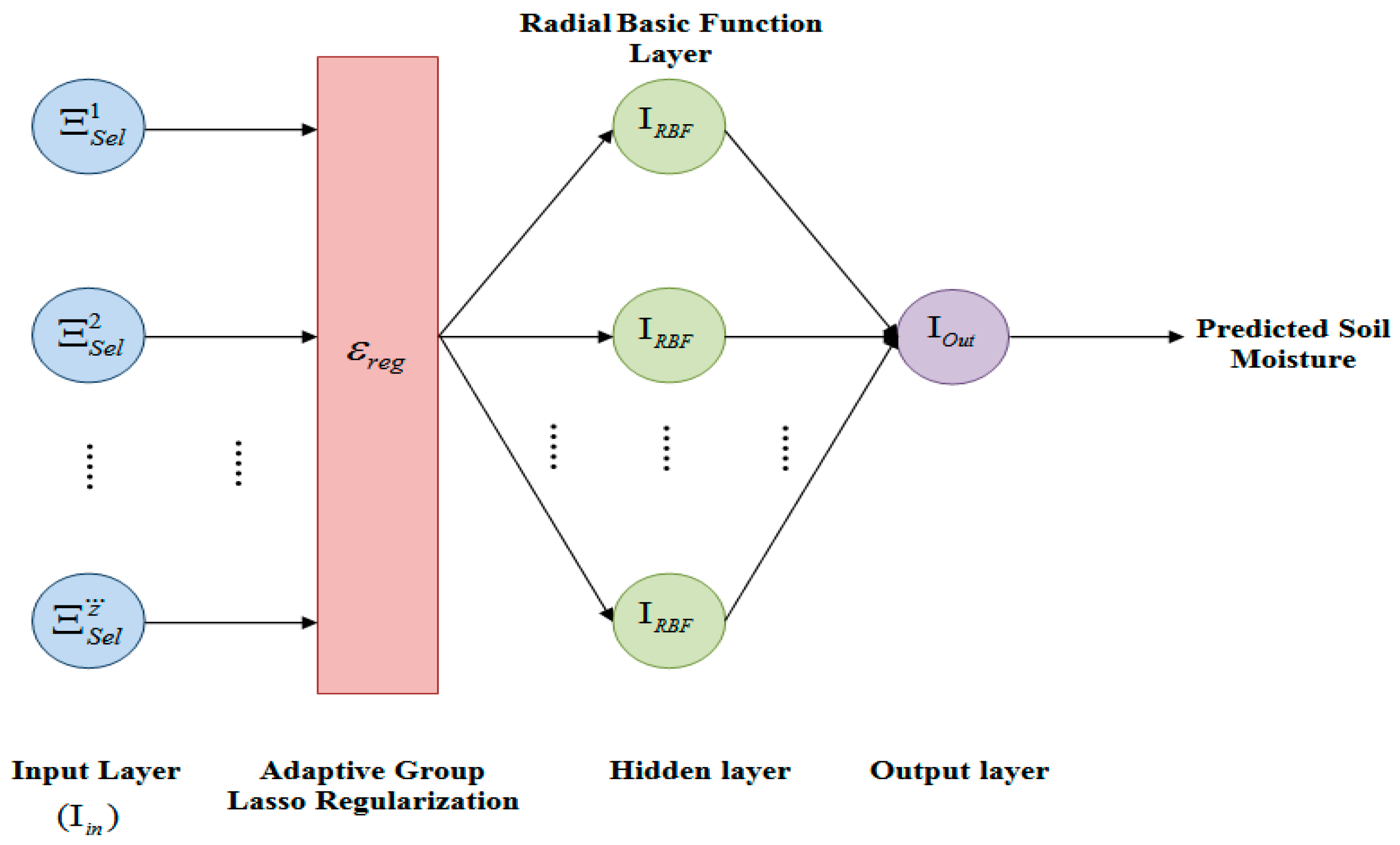
In this phase, the soil moisture is predicted from the selected optimal features $\left({\Xi }_{sel}\right)$ using AGRL-RBFN with IL. Radial Basis Function Networks (RBFNs) can be tailored to approximate diverse functions by adjusting the shape and parameters of the radial basis functions, enabling them to effectively model complex soil moisture dynamics and various influencing factors. However, the local relationship between input data and output predictions limited their ability to capture global patterns in soil moisture data, especially in datasets with significant variations. So, Adaptive Group Lasso Regularization (AGRL) is used in RBFN, which jointly regularizes feature groups and identifies crucial interactions for understanding soil moisture variations, particularly in remote sensing applications with related features. Additionally, IL is used, which enables models to update parameters with new data without retraining from scratch, benefiting soil moisture prediction, as conditions may change due to seasonal variations or climate shifts. The structural diagram of the proposed AGRL-RBFN classifier is depicted in Figure 2.

This classifier has the following input, adaptive group lasso regularization, hidden and output layers.

Input Layer

This layer receives the selected features $\left({\Xi }_{sel}\right)$ as input, and passed to the hidden layers. The inputs are represented as:

$${\mathrm{I}}_{in}\to \left\{{{\Xi }_{sel}}^1,{{\Xi }_{sel}}^2,\mathrm{.....}{{\Xi }_{sel}}^{\stackrel{⃛}{z}}\right\}$$

(27)

Where, $\left({\mathrm{I}}_{in}\right)$ indicates the inputs and has $\left(\stackrel{⃛}{z}\right)$ number of selected features $\left({\Xi }_{sel}\right)$.

Adaptive Group Lasso Regularization

To capture global patterns and regulate feature groups, AGRL is used. It regularizes the model based on feature groups, which helps capture interactions within these groups, particularly useful for remote sensing data. It is given by:

$${\epsilon }_{reg}=\underset{\upsilon }{\min }\left\{\widehat{L}\left(\upsilon \right)+\widehat{\lambda }{\displaystyle \sum _{e=1}^{\stackrel{⌢}{\mathrm{E}}}{\Gamma }_e{‖{\upsilon }_e‖}_2}\right\}$$

(28)

Here, $\left({\epsilon }_{reg}\right)$ defines the output of regularized feature group with loss function $\widehat{L}\left(\upsilon \right)$ of $\left({\mathrm{I}}_{in}\right)$, $\left(\upsilon \right)$ refers to the coefficient vector of $\left({\mathrm{I}}_{in}\right)$, $\left(\widehat{\lambda }\right)$ determines the regularization parameter, $\left({\Gamma }_e\right)$indicates the weight of group $\left(e\right)$, ${‖{\upsilon }_e‖}_2$ specifies L2 norm (Euclidean norm), and $\left(\stackrel{⌢}{\mathrm{E}}\right)$ is the number of feature groups.

Hidden Layer

Here, the regularized data $\left({\epsilon }_{reg}\right)$ are transformed using Radial Basis Functions (RBFs) (e.g., Gaussian function) to model non-linear relationships in soil moisture. The RBF $\left({\mathrm{I}}_{RBF}\right)$ is also called as activation function and is given by:

$${\mathrm{I}}_{RBF}=\exp \left(-{\displaystyle \frac{{‖{\epsilon }_{reg}-{\iota }_{ce{n}_n}‖}^2}{2{\sigma }_n^2}}\right)$$

(29)

Where, $\left({\iota }_{ce{n}_n}\right)$ refers to the$\left(n^{th}\right)$ centre of $\left({\mathrm{I}}_{RBF}\right)$, and $\left({\sigma }_n\right)$ indicates the $\left(n^{th}\right)$ width of the $\left({\mathrm{I}}_{RBF}\right)$.

Output Layer

In this layer, the output from the hidden layer is given to make the soil moisture prediction. The output $\left({\mathrm{I}}_{out}\right)$ of this layer is given by:

$${\mathrm{I}}_{out}={\displaystyle \sum _{\sout{n}=1}^{\stackrel{⃛}{\sout{l}}}{\Gamma }_{\sout{n}}•{\mathrm{I}}_{RBF}+{\tilde{b}}_{bias}}$$

(30)

Here, $\left({\tilde{b}}_{bias}\right)$ indicates the bias, $\left({\Gamma }_{\sout{n}}\right)$ refers to the weight of $\left({\sout{n}}^{th}\right)$ neuron, and $\left(\stackrel{⃛}{\sout{l}}\right)$ indicates the number of hidden neurons in RBF. From this output layer, the predicted soil moisture $\left({\mathrm{I}}_{out}\right)$ is obtained. The pseudocode for the AGRL-RBFN classifier is described as follows.

Pseudocode of AGRL-RBFN Input: Selected Features $\left({\Xi }_{sel}\right)$ Output: Predicted Soil Moisture $\left({\mathrm{I}}_{out}\right)$ Begin      Initialize $\left({\sigma }_n\right)$, $\left({\iota }_{ce{n}_n}\right)$      For each $\left({\mathrm{I}}_{in}\right)$           Compute ${\mathrm{I}}_{in}\to \left\{{{\Xi }_{sel}}^1,{{\Xi }_{sel}}^2,\mathrm{.....}{{\Xi }_{sel}}^{\stackrel{⃛}{z}}\right\}$           Regularize the input $\left({\mathrm{I}}_{in}\right)$                ${\epsilon }_{reg}=\underset{\upsilon }{\min }\left\{\widehat{L}\left(\upsilon \right)+\widehat{\lambda }{\displaystyle \sum _{e=1}^{\stackrel{⌢}{\mathrm{E}}}{\Gamma }_e{‖{\upsilon }_e‖}_2}\right\}$           Evaluate $\left({\mathrm{I}}_{RBF}\right)$           Calculate $\left({\mathrm{I}}_{out}\right)$                ${\mathrm{I}}_{out}={\displaystyle \sum _{\sout{n}=1}^{\stackrel{⃛}{\sout{l}}}{\Gamma }_{\sout{n}}•{\mathrm{I}}_{RBF}+{\tilde{b}}_{bias}}$           End for           Return$\to \left({\mathrm{I}}_{out}\right)$ End

Then, IL is applied to enable the model to adapt to new data, ensuring responsiveness to environmental changes while minimizing the loss function, which is essential for addressing seasonal and climate variations in soil moisture prediction. Finally, from the AGRL-RBFN classifier and IL approach the soil moisture is predicted effectively. The performance evaluation of the proposed soil moisture prediction system is discussed below.

3. Results and Discussion

In this section, the proposed system's performance is assessed and compared with existing models using a range of metrics. The evaluation results were derived from implementing and testing the framework on the PYTHON platform.

3.1. Dataset Description

The proposed approach for soil moisture monitoring is evaluated using data from the hyperspectral and soil-moisture dataset, which is mentioned in the reference section. This dataset, publicly available, which contains hyperspectral and soil moisture data collected during a 2017 field campaign in Karlsruhe. It includes variables such as datetime, soil moisture percentage, soil temperature, and spectral bands. The dataset is divided so that 80% is used for training, with the remaining 20% reserved for testing.

3.2. Performance Analysis

This section compares the performance of AdaK-MCC, FWFCSD, HCSWO, and AGRL-RBFN with existing models to showcase the improvements achieved by the proposed model

3.2.1. Performance Analysis of Gap Filling

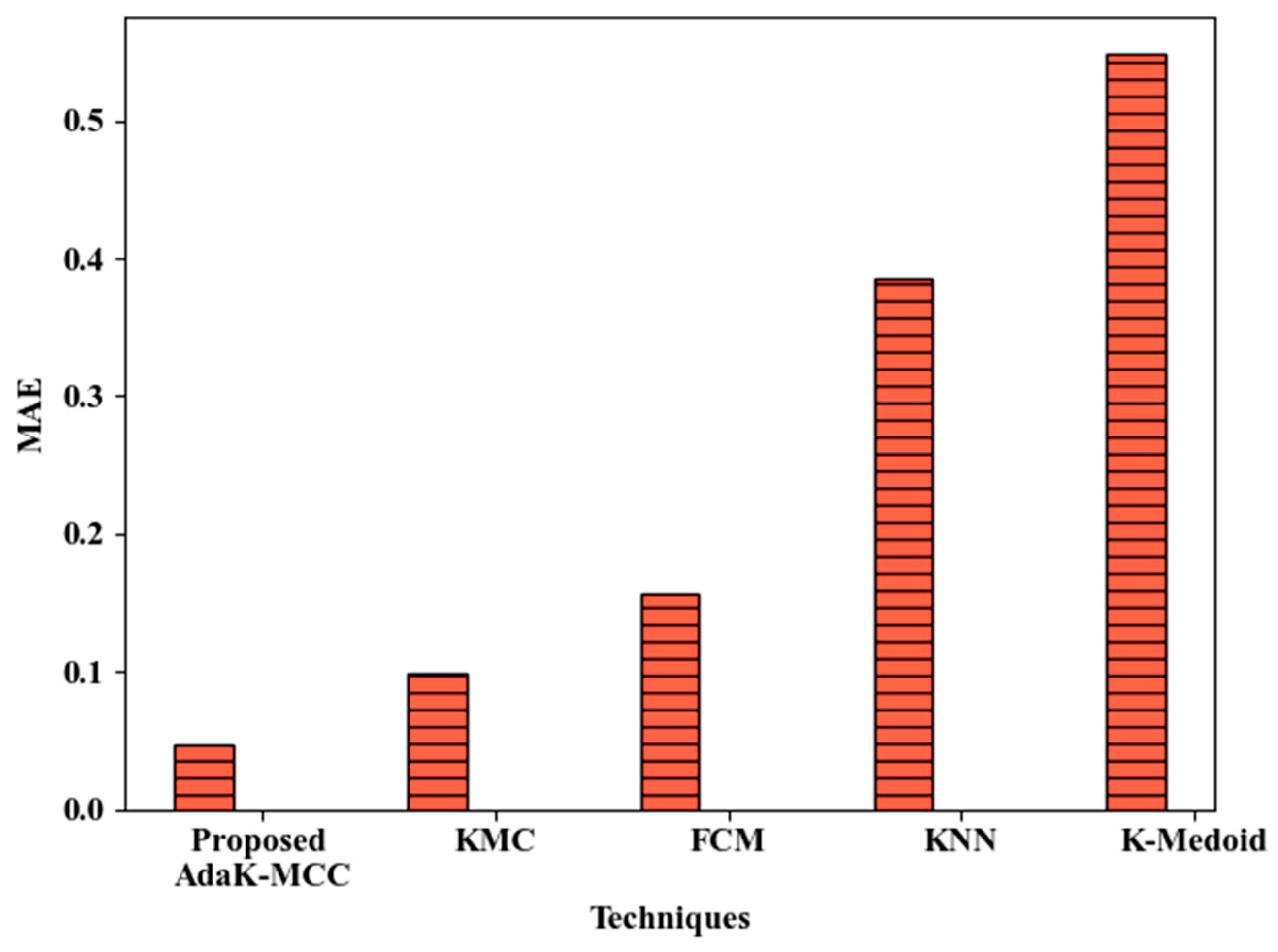
The performance evaluation of the proposed method AdaK-MCC for gap filling is discussed here. The graphical analysis of AdaK-MCC with existing KMC, Fuzzy C Means (FCM), K-Nearest Neighbor (KNN), K-Medoid in terms of Mean Absolute Error (MAE) is given below in Figure 3.

The gaps in the dataset are filled using AdaK-MCC technique with 0.047 of MAE. The proposed model obtained lower errors than the existing works. This is because the centroids are initialized using AMCs, which imputed the values effectively. The existing techniques such as KMC, FCM, KNN, and K-Medoid attained higher MAE of 0.099, 0.157, 0.386, and 0.548. Hence, the gaps were more efficiently filled than the existing models.

Table 1 shows the silhouette score of proposed AdaK-MCC and other existing techniques. The proposed technique achieved a silhouette score of 0.975. In contrast, the existing KMC, FCM, KNN, and K-Medoid attained 0.953, 0.929, 0.858, and 0.813 of silhouette score, which are lower than the proposed AdaK-MCC. This demonstrates the proposed approach's superiority in gap filling over existing models.

3.2.2. Performance Analysis of Clustering

In this section, the proposed AdaK-MCC is evaluated against existing clustering methods, including KMC, FCM, KNN, and K-Medoid, for a comprehensive clustering analysis.

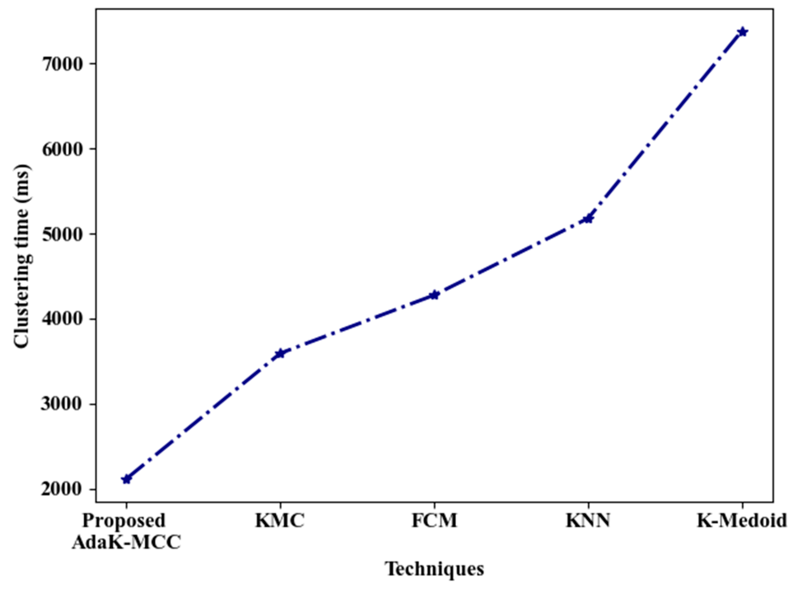
Figure 4 and Table 2 illustrate the performance analysis of AdaK-MCC compared to existing techniques Regarding clustering time and Dunn index. The AdaK-MCC attained a lower clustering time of 2118ms, and a higher Dunn index of 4.897. But the existing techniques KMC, FCM, KNN, and K-Medoid attained longer clustering times and lower Dunn index. This improved performance in the proposed technique is attributed to the centroid initialization using AMC technique. Thus, the robust performance of AdaK-MCC for data clustering is validated.

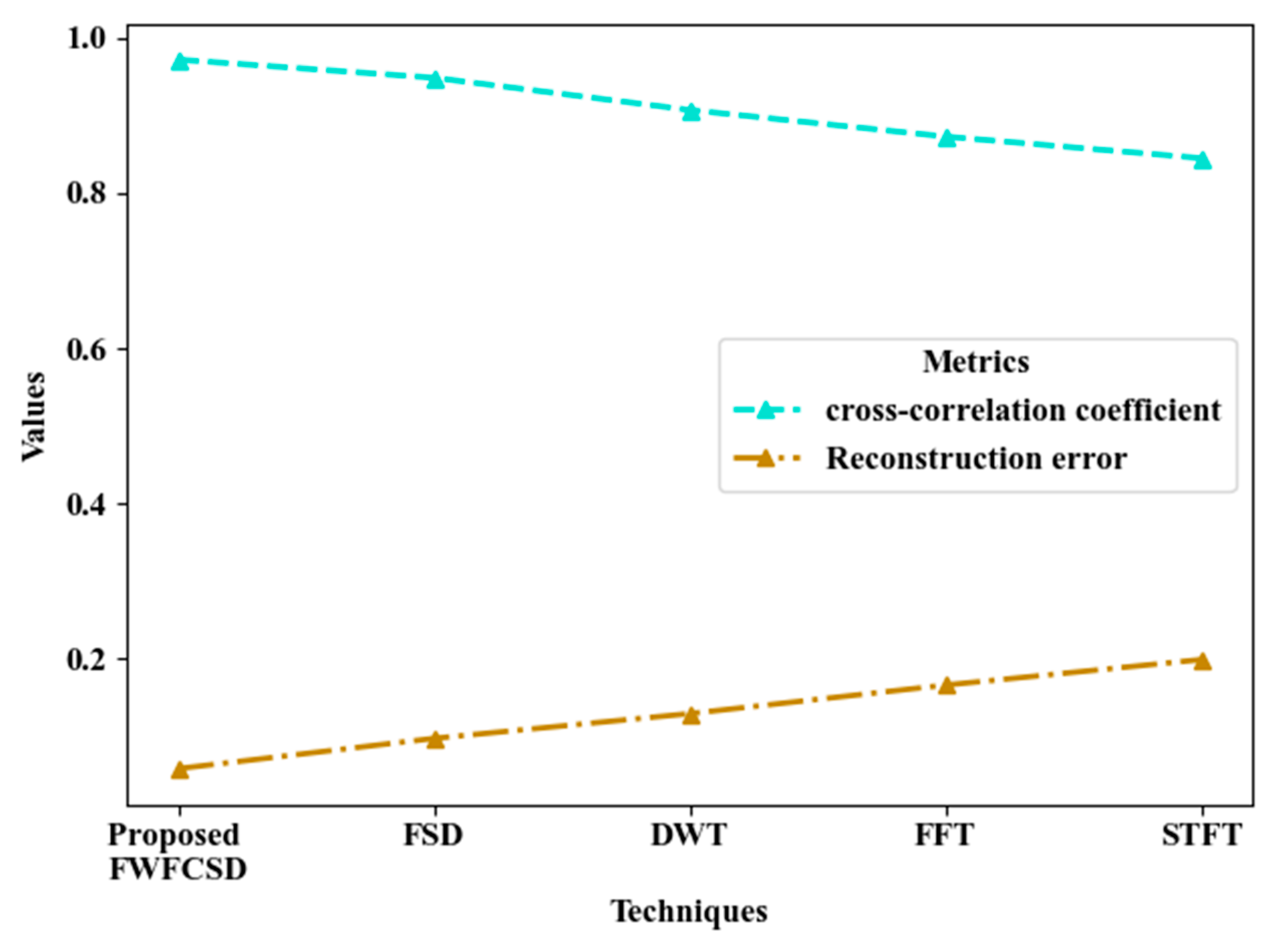
3.2.3. Performance Analysis of Varying Pattern Analysis

Here, the proposed FWFCSD is compared with the existing techniques like FSD, Discrete Fourier Transform (DFT), Fast Fourier Transform (FFT), Short Time Fourier Transform (STFT).

Figure 5 depicts the cross-correlation coefficient and reconstruction error of proposed FWFCSD and existing techniques. The varying patterns in the grouped seasons are analyzed by integrating FWFC for flexibly analyzing the varying soil moisture patterns. By integrating FWFC, the proposed FWFCSD achieved high cross-correlation coefficient of 0.9715 and low reconstruction error of 0.0589. Whereas, the existing FSD, DWT, FFT, STFT achieved an average cross-correlation coefficient of 0.893025 and an average reconstruction error of 0.148275, which are lower and higher than proposed FWFCSD. Therefore, the proposed FWFCSD showcases its efficacy in analyzing varying patterns.

Table 3 presents a performance analysis of the proposed FWFCSD method compared to existing techniques such as FSD, DWT, FFT, and STFT, focusing on execution time. The FWFCSD method achieved an execution time of just 18564ms, significantly outperforming the existing methods, which took 24796ms, 28357ms, 32497ms, and 39641ms, respectively. Thus, the proposed method provides a more effective analysis of the varying patterns compared to the existing methods.

3.2.4. Performance Analysis of Feature Selection

In this section, the performance evaluation of the proposed HCSWO in comparison to existing techniques is discussed, as outlined in Table 4.

The performance of the proposed method is expressed in Table 4 regarding feature selection time. To uniquely select the features, here, HCM is incorporated to cluster the correlated features to predict the moisture. It achieved lesser feature selection time of 2118ms. On the contrary, the existing methods such as SWO, Ant Colony Optimizer (ACO), Grey Wolf Optimizer (GWO), and Cuckoo Search Optimizer (CSO) consumed more feature selection time of 2211ms, 5178ms, 7135ms, and 9052ms. Hence, the proposed feature selection method demonstrates enhanced performance when compared to existing techniques.

3.2.5. Performance Analysis of Soil Moisture Prediction

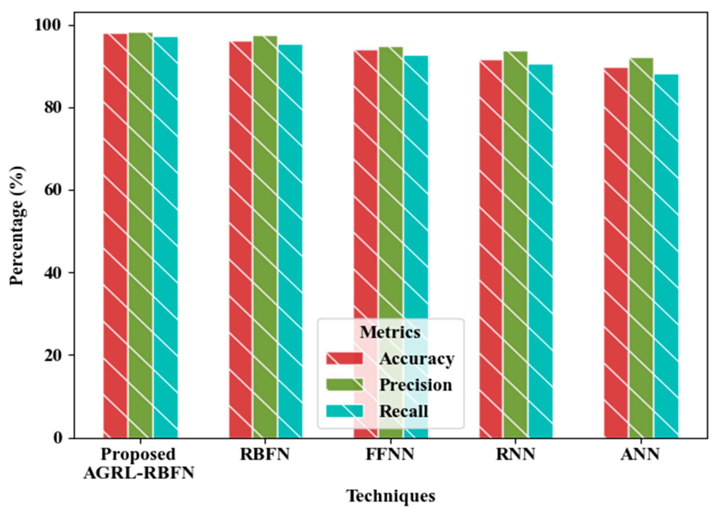
In this section, the performance of the proposed AGRL-RBFN is assessed in comparison to other relevant existing techniques.

Figure 6 and Figure 7 illustrate the performance of the proposed AGRL-RBFN in comparison to established techniques, including RBFN, Feed Forward Neural Network (FFNN), Recurrent Neural Network (RNN), and Artificial Neural Network (ANN). The AGRL-RBFN achieved an accuracy of 98.09%, precision of 98.17%, recall of 97.24%, F1-score of 98.95%, and specificity of 97.21%, all of which surpass the results of the existing methods. This superior performance can be attributed to the integration of AGRL within the RBFN, which effectively regularizes the feature groups for soil moisture prediction, in conjunction with the application of IL. In contrast, the traditional RBFN recorded accuracy, precision, and recall values of 96.27%, 97.55%, and 95.34%, respectively, which are inferior to those of the proposed AGRL-RBFN. Therefore, the proposed model demonstrates greater efficiency in predicting soil moisture compared to existing approaches.

Table 5 presents a comparison of the performance of the proposed AGRL-RBFN against existing methods, focusing on the False Positive Rate (FPR) and False Negative Rate (FNR). The proposed AGRL-RBFN achieved 0.0248 of FPR and 0.076 of FNR, which are lower than existing techniques. On the contrary, the existing techniques attained higher FPR and TNR. As a result, the proposed model outperformed the existing techniques in predicting soil moisture.

3.3. Comparison with Existing Approaches

This section provides a comparative evaluation of the proposed AGRL-RBFN against current methodologies for predicting soil moisture.

Table 6 provides a comparative evaluation of the proposed AGRL-RBFN against current methodologies for soil moisture prediction. The AGRL-RBFN technique demonstrates a high level of accuracy in forecasting soil moisture, thereby improving the overall effectiveness of the system; however, it does not specify appropriate crops for varying soil moisture conditions. In contrast, established methods such as Long Short-Term Memory (LSTM), Deep Convolutional Neural Networks (DCNNs), Attention-Aware LSTM, Deep Learning (DL) models utilizing Transfer Learning (TL), and Machine Learning (ML) regression with a pre-classification approach often encounter significant obstacles. These obstacles include substantial computational demands, limited generalizability, dependence on large datasets for training, and challenges in adjusting to swiftly changing climatic conditions. Consequently, the AGRL-RBFN exhibits superior performance in soil moisture prediction compared to these existing techniques.

4. Conclusions

Soil Moisture (SM) plays a critical role in fostering plant development and boosting agricultural productivity. A deficiency in soil moisture, whether in the short or long term, can adversely affect both rainfed and subsistence agricultural practices. As climate conditions evolve, the importance and difficulty of monitoring soil moisture will rise significantly. For plants to thrive, it is essential that soil moisture levels are maintained within an optimal range, avoiding extremes of saturation or drought. Excessively wet soils can result in the leaching of vital nutrients, while overly dry soils may lead to reduced crop yields and compromised quality.

Current research fails to sufficiently tackle the intricacies associated with forecasting soil moisture amid climatic changes, and it is deficient in providing thorough background information. This study introduced an effective system for predicting soil moisture utilizing AdaK-MCC, FWFCSD, HCSWO, and AGRL-RBFN. Initially, data collection was followed by a pre-processing phase where data gaps were addressed and seasonal clustering was performed using AdaK-MCC, achieving a mean absolute error (MAE) of 0.047 and a clustering duration of 2118 milliseconds. Subsequently, the varying patterns were examined through FWFCSD, which required an execution time of 18564 milliseconds. Following this, optimal features were identified from the extracted data within a feature selection timeframe of 2118 milliseconds using HCSWO. Ultimately, soil moisture predictions were made using AGRL-RBFN, resulting in an accuracy of 98.09%, precision of 98.17%, and an F1-score of 98.95%. The effectiveness of the proposed framework was further validated by comparing it with existing related approaches. Thus, the proposed model successfully predicted soil moisture levels.

In this study, the prediction of soil moisture has been addressed; however, the compatibility of particular crops with various soil types remains unexamined. Future research will focus on this aspect to enhance smart agricultural practices

References

- Abbes, A. Ben, Jarray, N., & Farah, I. R. (2024). Advances in remote sensing based soil moisture retrieval: applications, techniques, scales and challenges for combining machine learning and physical models. Artificial Intelligence Review, 57(9), 1–22. https://doi.org/10.1007/s10462-024-10734-1. [CrossRef]
- Adab, H., Morbidelli, R., Saltalippi, C., Moradian, M., & Ghalhari, G. A. F. (2020). Machine learning to estimate surface soil moisture from remote sensing data. Water (Switzerland), 12(11), 1–28. https://doi.org/10.3390/w12113223. [CrossRef]
- Babu, C. V. S., & Yadavamuthiah, K. (2024). Soil quality prediction using deep learning. Sustainable Development in AI, Blockchain, and E-Governance Applications, 171–188. https://doi.org/10.4018/979-8-3693-1722-8.ch010. [CrossRef]
- Celik, M. F., Isik, M. S., Yuzugullu, O., Fajraoui, N., & Erten, E. (2022). Soil Moisture Prediction from Remote Sensing Images Coupled with Climate, Soil Texture and Topography via Deep Learning. Remote Sensing, 14(21), 1–24. https://doi.org/10.3390/rs14215584. [CrossRef]
- Dabboor, M., Atteia, G., Meshoul, S., & Alayed, W. (2023). Deep Learning-Based Framework for Soil Moisture Content Retrieval of Bare Soil from Satellite Data. Remote Sensing, 15(7), 1–19. https://doi.org/10.3390/rs15071916. [CrossRef]
- Filipović, N., Brdar, S., Mimić, G., Marko, O., & Crnojević, V. (2022). Regional soil moisture prediction system based on Long Short-Term Memory network. Biosystems Engineering, 213, 30–38. https://doi.org/10.1016/j.biosystemseng.2021.11.019. [CrossRef]
- Hegazi, E. H., Samak, A. A., Yang, L., Huang, R., & Huang, J. (2023). Prediction of Soil Moisture Content from Sentinel-2 Images Using Convolutional Neural Network (CNN). Agronomy, 13(3), 1–18. https://doi.org/10.3390/agronomy13030656. [CrossRef]
- Jia, Y., Jin, S., Chen, H., Yan, Q., Savi, P., Jin, Y., & Yuan, Y. (2021). Temporal-Spatial Soil Moisture Estimation from CYGNSS Using Machine Learning Regression with a Preclassification Approach. IEEE Journal of Selected Topics in Applied Earth Observations and Remote Sensing, 14, 4879–4893. https://doi.org/10.1109/JSTARS.2021.3076470. [CrossRef]
- Kumar, P., Udayakumar, A., Anbarasa Kumar, A., Senthamarai Kannan, K., & Krishnan, N. (2023). Multiparameter optimization system with DCNN in precision agriculture for advanced irrigation planning and scheduling based on soil moisture estimation. Environmental Monitoring and Assessment, 195(1), 1–26. https://doi.org/10.1007/s10661-022-10529-3. [CrossRef]
- Lee, S. J., Choi, C., Kim, J., Choi, M., Cho, J., & Lee, Y. (2023). Estimation of High-Resolution Soil Moisture in Canadian Croplands Using Deep Neural Network with Sentinel-1 and Sentinel-2 Images. Remote Sensing, 15(16), 1–26. https://doi.org/10.3390/rs15164063. [CrossRef]
- Li, M., & Yan, Y. (2024). Comparative Analysis of Machine-Learning Models for Soil Moisture Estimation Using High-Resolution Remote-Sensing Data. Land, 13(8), 1–24. https://doi.org/10.3390/land13081331. [CrossRef]
- Li, Q., Wang, Z., Shangguan, W., Li, L., Yao, Y., & Yu, F. (2021). Improved daily SMAP satellite soil moisture prediction over China using deep learning model with transfer learning. Journal of Hydrology, 600, 1–14. https://doi.org/10.1016/j.jhydrol.2021.126698. [CrossRef]
- Li, Q., Zhu, Y., Shangguan, W., Wang, X., Li, L., & Yu, F. (2022). An attention-aware LSTM model for soil moisture and soil temperature prediction. Geoderma, 409, 1–17. https://doi.org/10.1016/j.geoderma.2021.115651. [CrossRef]
- Liu, J., Xu, Y., Li, H., & Guo, J. (2021). Soil moisture retrieval in farmland areas with sentinel multi-source data based on regression convolutional neural networks. Sensors (Switzerland), 21(3), 1–21. https://doi.org/10.3390/s21030877. [CrossRef]
- Liu, Q., Gu, X., Chen, X., Mumtaz, F., Liu, Y., Wang, C., Yu, T., Zhang, Y., Wang, D., & Zhan, Y. (2022). Soil Moisture Content Retrieval from Remote Sensing Data by Artificial Neural Network Based on Sample Optimization. Sensors, 22(4), 1–21. https://doi.org/10.3390/s22041611. [CrossRef]
- Liu, Q., Wu, Z., Cui, N., Jin, X., Zhu, S., Jiang, S., Zhao, L., & Gong, D. (2023). Estimation of Soil Moisture Using Multi-Source Remote Sensing and Machine Learning Algorithms in Farming Land of Northern China. Remote Sensing, 15(17), 1–22. https://doi.org/10.3390/rs15174214. [CrossRef]
- Nijaguna, G. S., Manjunath, D. R., Abouhawwash, M., Askar, S. S., Basha, D. K., & Sengupta, J. (2023). Deep Learning-Based Improved WCM Technique for Soil Moisture Retrieval with Satellite Images. Remote Sensing, 15(8), 1–17. https://doi.org/10.3390/rs15082005. [CrossRef]
- Pal, J., & Bodhe, H. (2023). Design and Implementation of Deep Learning Model For Soil Moisture Analysis . An IoT Based Soil Moisture Monitoring on Losant Platform. International Journal of Research in Engineering and Science, 11(4), 509–514.
- Patrizi, G., Bartolini, A., Ciani, L., Gallo, V., Sommella, P., & Carratu, M. (2022). A Virtual Soil Moisture Sensor for Smart Farming Using Deep Learning. IEEE Transactions on Instrumentation and Measurement, 71, 1–11. https://doi.org/10.1109/TIM.2022.3196446. [CrossRef]
- Peng, Y., Yang, Z., Zhang, Z., & Huang, J. (2024). A Machine Learning-Based High-Resolution Soil Moisture Mapping and Spatial–Temporal Analysis: The mlhrsm Package. Agronomy, 14(3), 1–23. https://doi.org/10.3390/agronomy14030421. [CrossRef]
- Roberts, T. M., Colwell, I., Chew, C., Lowe, S., & Shah, R. (2022). A Deep-Learning Approach to Soil Moisture Estimation with GNSS-R. Remote Sensing, 14(14), 1–29. https://doi.org/10.3390/rs14143299. [CrossRef]
- Shokati, H., Masha, M., Noroozi, A., & Abkar, A. A. (2024). Random Forest-Based Soil Moisture Estimation Using Sentinel-2, Landsat-8/9, and UAV-Based Hyperspectral Data. Remote Sensing, 16, 1–17.
- Singh, T., Kundroo, M., & Kim, T. (2024). WSN-Driven Advances in Soil Moisture Estimation: A Machine Learning Approach. Electronics (Switzerland), 13(8), 1–20. https://doi.org/10.3390/electronics13081590. [CrossRef]
- Uthayakumar, A., Mohan, M. P., Khoo, E. H., Jimeno, J., Siyal, M. Y., & Karim, M. F. (2022). Machine Learning Models for Enhanced Estimation of Soil Moisture Using Wideband Radar Sensor. Sensors, 22(15), 1–11. https://doi.org/10.3390/s22155810. [CrossRef]
- Wang, Y., Zhao, J., Guo, Z., Yang, H., & Li, N. (2023). Soil Moisture Inversion Based on Data Augmentation Method Using Multi-Source Remote Sensing Data. Remote Sensing, 15(7), 1–17. https://doi.org/10.3390/rs15071899. [CrossRef]
- Win, K., Sato, T., & Tsuyuki, S. (2024). Application of Multi-Source Remote Sensing Data and Machine Learning for Surface Soil Moisture Mapping in Temperate Forests of Central Japan. Information (Switzerland), 15(8), 1–25. https://doi.org/10.3390/info15080485. [CrossRef]
- Yang, Y., Li, H., Sun, M., Liu, X., & Cao, L. (2024). A Study on Hyperspectral Soil Moisture Content Pre-diction by Incorporating a Hybrid Neural Network into Stacking Ensemble Learning. Agronomy, 14(9), 1–17. https://doi.org/10.3390/agronomy14092054. [CrossRef]