
Submitted:
16 December 2024
Posted:
17 December 2024
You are already at the latest version
Abstract
Accurate knowledge of surface and subsurface soil moisture (SM) is essential for hydrologic modeling, weather forecasting, and agricultural water management. NASA’s Soil Moisture Active Passive (SMAP) satellite (level 3) provides ‘surface’ SM with 2–3 days temporal resolution, hence lacks daily and subsurface SM information. This study developed a convolutional neural network – long short-term memory (ConvLSTM) deep learning model to produce daily surface (5 cm) and subsurface (25 cm) SM products by integrating SMAP Level 3 ancillary data, North American Land Data Assimilation System Phase 2 (NLDAS-2) SM, and Soil Landscapes of the United States (SOLUS100) digital maps across the contiguous U.S. Two input scenarios were evaluated: scenario 1 used only SMAP ancillary data, and scenario 2 included both SMAP ancillary data and SOLUS100 soil maps. Model evaluation with in-situ SM data showed higher accuracy for scenario 2, indicating the importance of soil properties (texture and bulk density) in SM estimation. Coarse-textured soils showed the highest estimation accuracy, followed by medium- and fine-textured soils. The model also performed in estimating subsurface SM than surface SM for most land-cover types. Incorporating SMAP ancillary data and SOLUS100 digital soil maps into ConvLSTM improved surface and subsurface SM estimation. The results highlight the potential of deep learning for integrating multi-source multi-scale observations for improving SM estimation at large scale.
Keywords:
ConvLSTM
; Remote Sensing
; Soil moisture
; Soil Properties
; SOLUS100
1. Introduction
Soil Moisture (SM) is a key state variable that controls the exchange of water, energy, and carbon fluxes between the land surface and the atmosphere [1,2]. SM has numerous applications in hydrology, agriculture, and meteorology, such as irrigation management, drought monitoring [3], flood prediction [4], and weather forecasting [5]. However, accurate measurement and monitoring of SM in different spatial and temporal scales is still a challenge. While in situ SM networks such as International Soil Moisture Network (ISMN) provides more than 2,800 active stations, their spatial coverage is insufficient due to uneven distribution of the stations which limits their ability to represent the spatial variability of SM caused by heterogeneity of land surface factors, especially those related to soil and vegetation types [6].
During the past two decades, optical and thermal satellite remote sensing observations have been widely used for SM estimation due to their higher spatial resolution compared to microwave satellite observations [7,8,9,10]. These methods typically employ triangle or trapezoid models that use parameters such as land surface temperature – vegetation index [7,11] or shortwave infrared reflectance – vegetation index [12,13] to estimate SM. While these methods can provide SM estimates with high spatial resolution (20 to 500 m pixel size), they have limitations such as low penetration through vegetation canopies and reduced or irregular temporal resolution due to unstable atmospheric conditions (e.g., cloud cover, aerosols, etc.) [14]. In contrast, passive and active microwave satellite observations are unaffected by atmospheric conditions and their longer wavelengths enable deeper penetration through vegetation and soil surface. Microwave signals are highly sensitive to the dielectric properties of soil, which are primarily influenced by large dielectric constant of water [15,16]. NASA’s Soil Moisture Active Passive (SMAP) satellite was launched in 2015 to specifically measure global SM at L-band (1.4 GHz) within the top 5 cm of soil under various land covers with a spatial resolution of 9-36 km and a temporal resolution of 2-3 days using both descending (6:00 AM) and ascending (6:00 PM) overpasses [17]. SMAP passive observations in the form of brightness temperature are typically combined with other soil and vegetation attributes including scattering albedo, surface roughness, vegetation optical depth (VOD), and soil dielectric properties to estimate SM using the inversion of the tau-omega radiative transfer equation model, knows as zero-order model [18,19]. The tau-omega model is solved with the single channel algorithm (SCA) or the dual channel algorithm (DCA). In the SCA, brightness temperature observations at either horizontal (H) or vertical (V) polarization are used to retrieve SM, while the DCA uses both H and V polarizations to retrieve SM and VOD simultaneously [20,21]. The DCA generally yields more accurate results than the SCA, as it uses both polarizations and is currently the baseline algorithm to produce official SMAP SM products [22,23]. However, some studies have shown that the SCA-V algorithm may perform better under specific land covers [24,25]. Although SMAP primary product (Level 3) provides surface SM (top 5 cm) with a target unbiased root mean squared error of 0.04 cm3 cm-3 over areas with low vegetation water content (less than 0.5 kg m-2), it does not provide daily estimation and faces challenges in accurately retrieving SM in regions with dense vegetation cover, complex topography, and snow-covered soils [26]. Moreover, a limitation of the tau-omega model is that it does not account for temporal dynamics of vegetation and growth stages which may affect the accuracy of SM retrievals. The SMAP Level 4 SM product provides an average SM estimate from the surface down to 100 cm depth with a spatial resolution of 9 km and temporal resolution of 3-hours. This product is generated by assimilating SMAP brightness temperature observations into the NASA catchment land surface model [27]. Although this SM product has very high temporal resolution, its vertical resolution (within the soil profile) is course that limits its usefulness for applications that require surface, near-surface or root zone soil moisture information.
Alternative databases such as the North American Land Data Assimilation System phase-2 (NLDAS-2), which is the output of process-based models, offers SM estimates with high temporal resolution (hourly) and 0.125° (~12.5 km) spatial resolution for multiple soil layers [28]. However, the accuracy of this product is influenced by regional factors such as topographic complexity (TC), VOD, and uncertainties in model parameterization caused by the use of simplified representations of physical processes, such as one-dimensional vertical water flow in soil [29], which often lead to underestimation of SM during wet seasons and overestimation during dry conditions [30]. Despite such limitations, several studies have shown that NLDAS-2 SM outperforms SMAP SM estimates under forested and unforested land covers [31]. NLDAS-2 high temporal resolution and its ability to provide SM estimates for multiple soil layers give it an advantage, especially for root zone and profile SM monitoring where SMAP satellite observations, which primarily focus on the surface layer, are limited.
In recent years, machine learning and deep learning (DL) techniques have shown superior performance compared to traditional statistical and physical models [32]. These methods can be considered as an alternative to the direct SCA and DCA algorithms for SM estimation at large scale (33-38). The main advantage of DL methods includes their strong learning ability to find highly non-linear spatiotemporal relationships and capability to handle multi-source multi-scale observations [39]. In contrast, radiative transfer (e.g., SCA and DCA) and land surface models struggle to capture the inherent heterogeneity in soil and vegetation and the non-linear relationships between SM and land surface parameters [40]. The NLDAS-2 SM data can be used as the benchmark to train DL models for SM estimation as DL uses many neurons and hidden layers to identify complex patterns in the data, making them a highly promising approach for SM estimation [41,42]. However, much of the existing research on DL for SM estimation has focused on small scale modeling, which limits the ability to fully capture the intricate spatial and temporal non-linear relationships. Recently, studies presented a deep neural network that fuses SMAP ancillary variables with reanalysis SM data from ERA5 to produce a high accurate SMAP SM product for a wide range of land-covers and climate regimes [39]. The hybrid DL models such as Convolutional Neural Network – Long Short-Term Memory (ConvLSTM) has shown significantly better performance in this regard [43]. ConvLSTM combines the strengths of convolutional neural networks [44] for spatial feature extraction and long short-term memory (LSTM) networks [45] for capturing temporal dependencies. This enables ConvLSTM to concurrently model spatial and temporal variations in SM more effectively. As a result, ConvLSTM has gained attraction for estimating and forecasting of various hydrological variables, such as precipitation [46,47], evapotranspiration [48,49], flood [50], and streamflow [51].
Incorporating soil information (e.g., soil physical properties like texture) into machine learning and DL models significantly enhances SM estimation by enabling the models to capture complex relationship between soil characteristics and SM [52]. Soil texture, which affects the pore size distribution and water-holding capacity of soil, plays an important role in determining retention and movement of water within the soil profile [53]. By integrating soil physical properties like texture maps, especially the new released NRCS digital soil maps, as additional features, ConvLSTM can identify spatiotemporal patterns and correlations that contribute to more accurate estimates of SM. Moreover, including spatially distributed soil physical properties facilitates a better understanding of variability across different landscapes, improving model generalization and performance under diverse soil types, land covers, and climatic conditions.
This study aims to employe the ConvLSTM model to generate daily SM products for surface and subsurface soil by integrating multi-source multi-scale ground and satellite observations across the contiguous United States (CONUS). The specific objectives of this paper are: (i) to apply ConvLSTM for creating new surface and subsurface SM products by integrating SMAP SM and ancillary data, NRCS soil physical properties maps, and NLDAS-2 SM data, and (ii) to evaluate the accuracy of the new SM products with in-situ SM networks for different soil textural classes and land covers.
2. Materials and Methods
The Materials and Methods should be described with sufficient details to allow others to replicate and build on the published results. Please note that the publication of your manuscript implicates that you must make all materials, data, computer code, and protocols associated with the publication available to readers. Please disclose at the submission stage any restrictions on the availability of materials or information. New methods and protocols should be described in detail while well-established methods can be briefly described and appropriately cited.
2.1. SMAP Data and SOLUS100 Maps
The NASA’s Soil Moisture Active Passive (SMAP) mission was launched in 2015 to provide global SM estimates within the upper 5 cm soil. SMAP includes several SM products such as the Level 3 (L3) enhanced SM product with 9 km spatial and 2-3 days temporal resolution [19,54]. Here, we used SMAP L3 ancillary data including brightness temperature, albedo, effective SM, surface roughness, vegetation opacity, and vegetation water content as the ConvLSTM model inputs. These variables are currently used in the SMAP SM algorithms (e.g., DCA and SCA) to estimate surface SM. The SMAP L3 data (Version 6) were acquired from the National Snow and Ice Data Center (NSIDC) at EASE-Grid 2.0 Global projection (EPSG:6933) from January 2018 to December 2022.
Additionally, we used soil physical properties including texture (i.e., sand, silt and clay content) and bulk density from the USDA-NRCS Soil Landscapes of the United States (SOLUS100) maps. SOLUS100 is a new digital soil map generated from the fusion of soil profile data with field descriptions and soil survey maps via random forest modeling to provide high accurate physical and chemical soil properties maps at 100 m spatial resolution at seven standard soil depths (0, 5, 15, 30, 60, 100, and 150 cm) across the CONUS [55]. In this study, we used SOLUS100 maps for sand, silt, clay and bulk density properties for two depths, where the soil maps at 5 cm depth correspond to NLDAS-2 SM at 0-10 cm, and the maps at 30 cm depth correspond with NLDAS-2 SM at 10-40 cm.
2.2. Producing Benchmark Soil Moisture Data
To develop ConvLSTM models, we integrated two distinct SM products: SMAP SM (satellite product) and NLDAS-2 SM (process-based model) to leverage the strengths of both as pointed out above. Specifically, the SMAP Level 3 enhanced soil moisture product (SPL3SMP_E), which includes three SM products based on DCA, SCA-V, and SCA-H, and the NLDAS-2 Noah SM product at 0-10 cm and 10-40 cm depths [56], were utilized from January 1st, 2018, to December 30th, 2022. As mentioned above, there is no considerable study that compare the performance of SMAP SM products with other SM products such as NLDAS-2, as the performance is variable depending on land cover conditions [57]. Based on our validation results (Table 1), SMAP DCA SM demonstrated better correlations with ins-situ SM from both SCAN and USCRN networks, while the NLDAS-2 Noah SM showed better RMSE values across the CONUS. Therefore, the ConvLSTM model was designed to learn and produce new SM from the high correlation of SMAP DCA while consider low RMSEs from the NLDAS-2 Noah SM (depth 0-10 cm) for the surface depth (i.e., 5 cm). For the subsurface (i.e., 25 cm), the model relied solely on NLDAS-2 subsurface SM (10-40 cm) as SMAP Level 3 lacks SM data for subsurface soil. Recently, it has been demonstrated the applicability of integrating SMAP surface SM with reanalysis SM data from ERA5 to produce benchmark SM data for improving the training of deep neural networks over various land cover types across the CONUS [39].
To do so, the soil maps and NLDAS-2 data were resampled to a 9 km pixel size using bi-cubic (dis)aggregation method [58] to obtain a uniform spatial resolution based on SMAP L3 data. To preserve temporal continuity (i.e., 1 day), the SMAP data were gap-filled temporally using the Continuous Recurrent Unites (CRU) method prior to integration and subsequent processing using the ConvLSTM algorithm. The CRU is an encoder-decoder neural architecture designed to gaps in time series data by capturing temporal continuity between hidden states and optimally integrating noisy observations [59]. Figure 1 depicts the steps of data integration and deep learning modeling for surface and subsurface SM estimation with ConvLSTM model.
2.3. Model Input Scenarios
To estimate surface a subsurface SM, two scenarios were defined for each depth. While the SMAP ancillary data are used for both surface and subsurface and the two scenarios, for the surface (5 cm), the scenarios are based on whether soil physical attributes are included in the predictors or not. For the subsurface (25 cm), the scenarios are defined based on whether the generated surface SM is included as a predictor. These scenarios enable us to assess the effect and contribution of SMAP ancillary data and soil properties to estimating surface and subsurface SM. Table 2 summarizes the used scenarios and predictors for each soil depth.
2.4. ConvLSTM Model Architecture and Development
To estimate SM, we integrated convolutional neural network with long short-term memory network, named as ConvLSTM, to identify both spatial and temporal patterns in SM dynamics and high nonlinear relationships between SM and the predictors. The ConvLSTM is mathematically defined as follows [43].
where is the current input at time step , is the previous hidden state (short-term memory), is the previous cell state (long-term memory), , , and are forget, input and output gates, respectively, is the candidate cell sate, W are the network weights, are the biases, is the sigmoid activation function, is the hyperbolic tangent activation function, denotes the convolution operation, and represents element-wise multiplication. At each time step , the network outputs a value () which is compared to the reference soil moisture data to compute the loss and update the network weights during training.
As shown in Figure 1, after unifying data (i.e., gap-filling, resampling, and reprojecting), each predictor was reshaped into thousands of smaller images to expedite the execution of the ConvLSTM and enhance the model’s capability to capture parameter variations [43]. Subsequently, the predictors were organized into sequences of three consecutive days (lookback: 3) to better explore the temporal relationships [60]. The dataset was split into training (years of 2018 to 2020), validation (year 2021), and testing (year 2022) sets which approximately correspond to 60% training, 20% validation, and 20% testing.
The developed ConvLSTM model consists of ten layers with varying number of filters (i.e., 16, 32, 48, and 64) in each layer, capturing progressively more complex spatiotemporal patterns as data passes through the layers [43]. The kernel size was set as 3, the activation function as ‘sigmoid’, padding as ‘same’, and optimizer as ‘Adam’. A dropout rate of 0.2 was used after each layer along with early stopping to prevent overfitting [61]. Batch normalization was applied after each layer to stabilize and accelerate the training process. Moreover, the model was equipped with two Attention Blocks after the second and fifth layers that enables the model to focus on important features in both spatial and temporal dimensions [62]. Each attention block performs global average pooling operation to summarize features across spatial dimensions, followed by two dense layers that first reduce the number of features and then restore them to the original size, generating attention weights. These weights are then multiplied by the original inputs to assign higher importance to more important features and enable the model to focus on key spatial patterns [64]. As mentioned above, to develop ConvLSTM model, we used the SMAP SM and NLDAS-2 SM products as benchmark data. For the surface depth, this was based on the NLDAS-2’s low RMSE values and the SMAP DCA SM’s high correlation with in-situ SM measurements. Hence, we defined the loss function to minimize both the RMSE and (1-R2) between the model outputs and SMAP and NLDAS-2 SM products, respectively, as formulated in the following equation.
where and are the weight parameters set to unity. For estimating subsurface SM, the loss function specifically focuses on minimizing RMSE values between the model outputs and NLDAS-2 SM, as there is no SMAP SM product available for the subsurface soil layer.
2.6. In Situ SM and Model Validation
The performance of the developed ConvLSTM models for surface and subsurface SM estimation was assessed using in-situ SM measurements from the Soil Climate Analysis Network (SCAN) [65] and the U.S. Climate Reference Network (USCRN) [66] for depths of 5-, 10-, and 20- cm for the testing set (year 2022). To further evaluate the model performance in different land-cover types and soil textures, we used MODIS satellite land-cover product (MCD12Q1) [67] and SOLUS100-based soil textural classes based on USDA classification scheme. The locations of in-situ stations along with the distribution of soil texture classes are displayed in Figure 2. The error metrics including root mean squared error (RMSE), mean bias error (Bias) and unbiased RMSE (ubRMSE) were used.
3. Results and Discussion
In this section, we first evaluate the performance of the ConvLSTM model for surface and subsurface soil moisture estimation based on two sets/scenarios of predictors and then examine the model performance for various soil textural classes and land cover types across the CONUS.
3.1. Surface and Subsurface SM Estimations with ConvLSTM
As explained above, two different scenarios including SMAP ancillary data with and without soil physical attributes from SOULS100 maps were considered for SM estimation in each soil depth. When comparing the overall performance of the ConvLSTM model for each scenario, we found that the second scenario, which includes SOLUS100 data, outperformed the first scenario (Table 3), revealing that soil physical properties including sand, silt, clay content and bulk density play an important role in spatiotemporal SM estimation even when the maps are aggregated to coarse pixels with 9-km size at large scale. The importance of soil physical properties in SM estimation and monitoring has been shown in other studies [52,68,69,70]. The mean R and ubRMSE values for the surface depth and for scenarios 1 and 2 were 0.54 and 0.053 cm3 cm-3, indicating similar accuracy for the two scenarios. For the subsurface depth, scenario 2 slightly outperformed scenario 1 with mean R and ubRMSE values of 0.45 and 0.043 cm3 cm-3 (scenario 1) and 0.51 and 0.041 cm3 cm-3 (scenario 2) respectively. This could be due to including the estimated surface soil moisture as an additional input (see Table 2). The mean ubRMSE values meet the target accuracy for SMAP SM products (i.e., ubRMSE of 0.04 cm3 cm-3) for vegetation water content less than 0.5 kg m-2 [54] however the ConvLSTM SM estimates include advantages like daily SM for surface and subsurface soil depths. Though the ConvLSTM model was trained with both NLDAS-2 SM and SMAP L3 SM data, it still provides acceptable accuracy for estimating surface and subsurface SM.
3.2. Effects of Soil Texture on Soil Moisture Estimation
To better determine the effect of soil texture on the accuracy of SM estimation with the ConvLSTM model, we further classified the twelve soil textural classes (Figure 2) into three major classes: fine-textured (sandy clay, silty clay, and clay), medium-textured (loam, clay loam, silt loam, sandy clay loam, silty clay loam, silt) and coarse-textured (sand, loamy sand, and sandy loam) soils [70]. This grouping reduces the complexity of the soil texture classes for interpreting the results and helps identify general trends in SM estimation. The estimated SM was evaluated within each soil texture group against in-situ SM measurements from both SCAN and USCRN. The boxplots shown in Figure 3 display the error metrics of SM estimates for the surface and subsurface depths for the three groups of soil texture. As seen, based on the ubRMSE values, the accuracy of SM estimates for coarse-textured soils is slightly higher than that of medium-textured soils, followed by fine-textured soils. This could be partly attributed to the narrow range of SM content in coarse-textured soils due to their smaller porosity (i.e., saturation water content) and low water holding capacity. Similarly, the mean ubRMSE values for the surface depth are slightly lower than those of NLDAS-2 SM for fine- and coarse-textured soils, while no difference was observed for the subsurface SM estimates between the ConvLSTM and NLDAS-2. Based on the correlation coefficient (R) values, the model performed better for fine-textured soils, followed by medium-textured soils. The model performed slightly better for estimating subsurface SM compared to surface SM, which could be attributed to the lower dynamics of SM in deeper soil layers. By comparing scenarios 1 and 2, it is observed that the model performed slightly better in terms of ubRMSE for scenario 2 in medium- and fine-textured soils, while no significant improvement was observed between scenarios 1 and 2 for coarse-textured soils. Recently, SMAP level 3 SM products have been tested for estimating soil texture in China [71], which indicates the potential of SMAP SM data as an indirect method for characterizing soil physical properties at global scale.
3.3. Effects of Land Cover Types on Soil Moisture Estimation
Figure 4 displays the error metrics for surface and subsurface SM estimates calculated over various land-cover types against in-situ SM measurements from SCAN and USCRN networks for the test set. Overall, in terms of R and ubRMSE values, the model performed better for estimating subsurface SM than surface SM for most land-cover types, where the lower unRMSE values were obtained over savanna and woody savanna land-covers, followed by grasslands. Compared to the NLDAS-2 SM product, the ConvSLTM model performed better in terms of R values over shrublands, croplands, permanent wetland, savanna, and woody savannas. Regarding ubRMSE, the model outperformed NLDAS-2 SM product in permanent wetlands, savanna and woody savanna. In terms of ubRMSE values, the model estimates from scenario 2 outperformed scenario 1 estimates over permanent wetlands and savanna land-covers, while both scenarios performed similarly over croplands and shrublands. In grasslands and woody savannas, scenario 1 outperformed scenario 2. Over croplands, as a major land-cover type, and in terms of R and RMSE values, the ConvLSTM for both scenarios 1 and 2 performed better than that of NLDAS-2 SM product, though the model was trained based on NLDAS-2 SM products. In terms of mean bias, the ConvLSTM model shows the smallest values for surface and subsurface depths in most land-cover types, especially in croplands, shrublands and savanna. However, due to low learning ability of the model or low accuracy of NLDAS-2 SM products, the bias is large in other land covers like grasslands and permanent wetlands.
3.4. Spatiotemporal Validation of Soil Moisture Estimates
We further evaluated the accuracy of SM estimates from scenario 2 with in-situ SM measurements across the CONUS. Here, we are showing the result only for scenario 2 as it outperformed scenario 1 in most cases because of the effect of soil physical attributes and incorporating estimated surface SM as an additional predictor for subsurface SM estimation. Figure 5 illustrates the spatial patterns of the error metrics for each method, showing good agreement between the estimated and measured SM in terms of all error metrics for most of the stations, especially in western, northwest and southwest of the CONUS, where the model resulted in median R values of 0.5 and median ubRMSE values of 0.05 cm3 cm-3 (surface depth) and 0.04 cm3 cm-3 (subsurface depth). For example, in Utah state where the density of ground stations is high and because of topography the SMAP SM struggle to effectively capture variability [36], the model performed well. However, the bias values are large (more negative) in the southeast and mid-west regions, indicating that the model tends to underestimate surface and subsurface SM in these regions, while overestimating in the western CONUS areas. Based on the histograms of R and ubRMSE values, the model performed slightly better for estimating SM in the subsurface than the surface layer.
In Figure 6, all SM estimates from the ConvLSTM model based on scenario 2 for surface and subsurface depths are plotted and compared with the in-situ SM measurements. As shown, the performance for surface and subsurface depths is approximately similar, with correlation values of 0.72 and 0.75 and RMSE values of 0.09 and 0.10 cm3 cm-3 for surface and subsurface depths, respectively. Visually, the model overestimates SM for dry conditions while underestimates SM for wet conditions.
To better understand the performance of the ConvLSTM model for temporal estimation of SM, we plotted the estimated surface and subsurface SM against in-situ measurements from three SCAN sites covered by cropland, grassland, and savanna land-covers across sandy loam (coarse-textured) and silt loam (medium-textured) soils. As shown in Figure 7, SM estimates from both scenarios well capture in-situ SM temporal dynamics, especially at low SM values, and clearly respond to precipitation events. For the selected three sites, the SM estimates and NLDAS-2 SM underestimate in-situ measurements, particularly in wet soil conditions. With respect to the cumulative density function (CDF) curves, the ConvLSTM model underestimates SM in humid sites while slightly overestimates SM in dry sites. In addition, scenario 2 slightly outperformed scenario 1 in both selected sites in arid and humid conditions.
4. Summary and Conclusions
Accurate information about surface and subsurface soil moisture (SM) with adequate temporal resolution (e.g., daily) at large scale is critical for a range of applications in hydrology, weather, and agriculture. Advances in deep learning techniques for data fusion and spatiotemporal modeling offer exceptional opportunity for integrating multi-source multi-scale data and capturing complex spatial and temporal relationships between SM and land surface parameters.
In this study, we developed a new method for estimating surface and subsurface SM using convolutional neural network and long short-term memory (ConvLSTM) deep learning techniques. ConvLSTM can capture both spatial and temporal nonlinearities, making the method ideal for modeling the intricate dynamics of SM. To do so, we implemented a method that integrates SMAP satellite SM and its ancillary variables with process-based NLDAS-2 SM products. This fusion leverages the strengths of both datasets, enabling the daily estimation of surface (5-cm) and subsurface (25-cm) SM. We employed ConvLSTM model in conjunction with two scenarios of inputs: (1) SMAP ancillary data, and (2) SMAP ancillary data with soil physical attributes from SOLUS100 digital maps. We further evaluated the effect of including surface SM estimates for estimating subsurface SM. The predictors included SMAP ancillary data like brightness temperature, albedo, soil temperature, surface roughness coefficient, vegetation opacity, and vegetation water content, in conjunction with SOLUS100-based soil physical properties. The model was trained using SMAP DCA and NLDAS-2 SM products, aiming to maximize correlation (R) and minimize RMSE, respectively. Extensive validation using in-situ SM data from SCAN and USCRN stations across the CONUS demonstrated that the ConvLSTM model achieved high accuracy for both surface and subsurface SM, closely aligning with observed data. The inclusion of soil properties (i.e., sand, silt, clay and bulk density) significantly enhanced model performance, particularly in coarse-textured soils and cropland areas, where the model exhibited low unbiased RMSE (ubRMSE) values. Additionally, the model showed superior performance in estimating subsurface SM compared to surface SM, especially when surface SM estimates are used as an additional predictor, across various land-covers, especially in areas covered by savanna and woody savanna.
The proposed approach overcomes the limitations of SMAP satellite 2-3 days overpasses, provides daily SM estimates for surface and subsurface, and reduces the extensive input requirements typical of process-based models. Consequently, this integration facilitates the production of comprehensive global SM estimates for both surface and subsurface depths. It highlights the effectiveness of integrating satellite-based and process-based SM retrieval methods within a ConvLSTM deep learning framework for robust SM estimation at large scale.
Author Contributions
S.R.: Conceptualization, methodology, formal analysis, investigation, writing-original draft; E.B.: Conceptualization, methodology, investigation, writing-review and editing, supervision, project administration, and funding acquisition; S.G.: Conceptualization, methodology, investigation, writing-review and editing, supervision, and funding acquisition. All authors have read and agreed to the published version of the manuscript.
Funding
The authors gratefully acknowledge funding from the U.S. Department of Agriculture Natural Resources Conservation Service (USDA-NRCS) Soil Science Division under grant #NR223A750025C007, and by the USDA NIFA Hatch/Multi-State/NRS project # FLA-SWS-006588 and FLA-SWS-006559.
Data Availability Statement
All data analyzed or generated in the course of the presented study are available from the authors upon request.
Acknowledgments
In this section, you can acknowledge any support given which is not covered by the author contribution or funding sections. This may include administrative and technical support, or donations in kind (e.g., materials used for experiments).
The authors gratefully acknowledge the support from Dr. Suzann Kienast who provided valuable guidance for using the SOLUS100 digital soil maps in this project.
Conflicts of Interest
The authors declare no conflicts of interest.
References
- Vereecken, H.; Schnepf, A.; Hopmans, J.W.; Javaux, M.; Or, D.; Roose, T.; Vanderborght, J.; Young, M.H.; Amelung, W.; Aitkenhead, M. Modeling Soil Processes: Review, Key Challenges, and New Perspectives. Vadose zone journal 2016, 15, vzj2015-09. [Google Scholar] [CrossRef]
- Babaeian, E.; Sadeghi, M.; Jones, S.B.; Montzka, C.; Vereecken, H.; Tuller, M. Ground, Proximal, and Satellite Remote Sensing of Soil Moisture. Reviews of Geophysics 2019, 57, 530–616. [Google Scholar] [CrossRef]
- Narasimhan, B.; Srinivasan, R. Development and Evaluation of Soil Moisture Deficit Index (SMDI) and Evapotranspiration Deficit Index (ETDI) for Agricultural Drought Monitoring. Agric For Meteorol 2005, 133, 69–88. [Google Scholar] [CrossRef]
- Norbiato, D.; Borga, M.; Degli Esposti, S.; Gaume, E.; Anquetin, S. Flash Flood Warning Based on Rainfall Thresholds and Soil Moisture Conditions: An Assessment for Gauged and Ungauged Basins. J Hydrol (Amst) 2008, 362, 274–290. [Google Scholar] [CrossRef]
- Koster, R.D.; Dirmeyer, P.A.; Guo, Z.; Bonan, G.; Chan, E.; Cox, P.; Gordon, C.T.; Kanae, S.; Kowalczyk, E.; Lawrence, D. Regions of Strong Coupling between Soil Moisture and Precipitation. Science (1979) 2004, 305, 1138–1140. [Google Scholar] [CrossRef]
- Dorigo, W.A.; Wagner, W.; Hohensinn, R.; Hahn, S.; Paulik, C.; Xaver, A.; Gruber, A.; Drusch, M.; Mecklenburg, S.; Van Oevelen, P. The International Soil Moisture Network: A Data Hosting Facility for Global in Situ Soil Moisture Measurements. Hydrol Earth Syst Sci 2011, 15, 1675–1698. [Google Scholar] [CrossRef]
- Carlson, T. An Overview of the” Triangle Method” for Estimating Surface Evapotranspiration and Soil Moisture from Satellite Imagery. Sensors 2007, 7, 1612–1629. [Google Scholar] [CrossRef]
- Wang, W.; Huang, D.; Wang, X.-G.; Liu, Y.-R.; Zhou, F. Estimation of Soil Moisture Using Trapezoidal Relationship between Remotely Sensed Land Surface Temperature and Vegetation Index. Hydrol Earth Syst Sci 2011, 15, 1699–1712. [Google Scholar] [CrossRef]
- Shafian, S.; Maas, S.J. Index of Soil Moisture Using Raw Landsat Image Digital Count Data in Texas High Plains. Remote Sens (Basel) 2015, 7, 2352–2372. [Google Scholar] [CrossRef]
- Rabiei, S.; Jalilvand, E.; Tajrishy, M. A Method to Estimate Surface Soil Moisture and Map the Irrigated Cropland Area Using Sentinel-1 and Sentinel-2 Data. Sustainability 2021, 13, 11355. [Google Scholar] [CrossRef]
- Moran, M.S.; Clarke, T.R.; Inoue, Y.; Vidal, A. Estimating Crop Water Deficit Using the Relation between Surface-Air Temperature and Spectral Vegetation Index. Remote Sens Environ 1994, 49, 246–263. [Google Scholar] [CrossRef]
- Sadeghi, M.; Babaeian, E.; Tuller, M.; Jones, S.B. The Optical Trapezoid Model: A Novel Approach to Remote Sensing of Soil Moisture Applied to Sentinel-2 and Landsat-8 Observations. Remote Sens Environ 2017, 198, 52–68. [Google Scholar] [CrossRef]
- Babaeian, E.; Tuller, M. The Feasibility of Remotely Sensed Near-Infrared Reflectance for Soil Moisture Estimation for Agricultural Water Management. Remote Sens (Basel) 2023, 15, 2736. [Google Scholar] [CrossRef]
- Zhao, W.; Li, Z.-L. Sensitivity Study of Soil Moisture on the Temporal Evolution of Surface Temperature over Bare Surfaces. Int J Remote Sens 2013, 34, 3314–3331. [Google Scholar] [CrossRef]
- Ulaby, F.T. Microwave Remote Sensing, Active and Passive. Microwave Remote Sensing Fundamentals and Radiometry 1981, 1, 191–208. [Google Scholar]
- Mironov, V.L.; Kosolapova, L.G.; Fomin, S. V Physically and Mineralogically Based Spectroscopic Dielectric Model for Moist Soils. IEEE Transactions on Geoscience and Remote Sensing 2009, 47, 2059–2070. [Google Scholar] [CrossRef]
- Entekhabi, D.; Njoku, E.G.; O’neill, P.E.; Kellogg, K.H.; Crow, W.T.; Edelstein, W.N.; Entin, J.K.; Goodman, S.D.; Jackson, T.J.; Johnson, J. The Soil Moisture Active Passive (SMAP) Mission. Proceedings of the IEEE 2010, 98, 704–716. [Google Scholar] [CrossRef]
- Park, C.-H.; Jagdhuber, T.; Colliander, A.; Lee, J.; Berg, A.; Cosh, M.; Kim, S.-B.; Kim, Y.; Wulfmeyer, V. Parameterization of Vegetation Scattering Albedo in the Tau-Omega Model for Soil Moisture Retrieval on Croplands. Remote Sens (Basel) 2020, 12, 2939. [Google Scholar] [CrossRef]
- Li, X.; Wigneron, J.-P.; Fan, L.; Frappart, F.; Yueh, S.H.; Colliander, A.; Ebtehaj, A.; Gao, L.; Fernandez-Moran, R.; Liu, X. A New SMAP Soil Moisture and Vegetation Optical Depth Product (SMAP-IB): Algorithm, Assessment and Inter-Comparison. Remote Sens Environ 2022, 271, 112921. [Google Scholar] [CrossRef]
- Njoku, E.G.; Jackson, T.J.; Lakshmi, V.; Chan, T.K.; Nghiem, S. V Soil Moisture Retrieval from AMSR-E. IEEE transactions on Geoscience and remote sensing 2003, 41, 215–229. [Google Scholar] [CrossRef]
- Gao, L.; Ebtehaj, A.; Chaubell, M.J.; Sadeghi, M.; Li, X.; Wigneron, J.-P. Reappraisal of SMAP Inversion Algorithms for Soil Moisture and Vegetation Optical Depth. Remote Sens Environ 2021, 264, 112627. [Google Scholar] [CrossRef]
- Chan, S.K.; Bindlish, R.; O’Neill, P.E.; Njoku, E.; Jackson, T.; Colliander, A.; Chen, F.; Burgin, M.; Dunbar, S.; Piepmeier, J. Assessment of the SMAP Passive Soil Moisture Product. IEEE Transactions on Geoscience and Remote Sensing 2016, 54, 4994–5007. [Google Scholar] [CrossRef]
- O’Neill, P.; Bindlish, R.; Chan, S.; Njoku, E.; Jackson, T. Algorithm Theoretical Basis Document. Level 2 & 3 Soil Moisture (Passive) Data Products. 2018.
- Chan, S.K.; Bindlish, R.; O’Neill, P.; Jackson, T.; Njoku, E.; Dunbar, S.; Chaubell, J.; Piepmeier, J.; Yueh, S.; Entekhabi, D.; et al. Development and Assessment of the SMAP Enhanced Passive Soil Moisture Product. Remote Sens Environ 2018, 204, 931–941. [Google Scholar] [CrossRef]
- Chen, Y. , Li, L., Whiting, M., Chen, F., Sun, Z., Song, K., & Wang, Q. Convolutional neural network model for soil moisture prediction and its transferability analysis based on laboratory Vis-NIR spectral data. International Journal of Applied Earth Observation and Geoinformation, 2021,104, 102550.
- Dorigo, W.; Wagner, W.; Albergel, C.; Albrecht, F.; Balsamo, G.; Brocca, L.; Chung, D.; Ertl, M.; Forkel, M.; Gruber, A. ESA CCI Soil Moisture for Improved Earth System Understanding: State-of-the Art and Future Directions. Remote Sens Environ 2017, 203, 185–215. [Google Scholar] [CrossRef]
- Reichle, R.H.; Liu, Q.; Koster, R.D.; Crow, W.T.; De Lannoy, G.J.M.; Kimball, J.S.; Ardizzone, J. V; Bosch, D.; Colliander, A.; Cosh, M. Version 4 of the SMAP Level--4 Soil Moisture Algorithm and Data Product. J Adv Model Earth Syst 2019, 11, 3106–3130. [Google Scholar] [CrossRef]
- Xia, Y.; Mitchell, K.; Ek, M.; Sheffield, J.; Cosgrove, B.; Wood, E.; Luo, L.; Alonge, C.; Wei, H.; Meng, J. Continental--scale Water and Energy Flux Analysis and Validation for the North American Land Data Assimilation System Project Phase 2 (NLDAS--2): 1. Intercomparison and Application of Model Products. Journal of Geophysical Research: Atmospheres 2012, 117. [Google Scholar] [CrossRef]
- Balsamo, G.; Beljaars, A.; Scipal, K.; Viterbo, P.; van den Hurk, B.; Hirschi, M.; Betts, A.K. A Revised Hydrology for the ECMWF Model: Verification from Field Site to Terrestrial Water Storage and Impact in the Integrated Forecast System. J Hydrometeorol 2009, 10, 623–643. [Google Scholar] [CrossRef]
- Xia, Y.; Ek, M.B.; Wu, Y.; Ford, T.; Quiring, S.M. Comparison of NLDAS-2 Simulated and NASMD Observed Daily Soil Moisture. Part I: Comparison and Analysis. J Hydrometeorol 2015, 16, 1962–1980. [Google Scholar] [CrossRef]
- Ayres, E.; Reichle, R.H.; Colliander, A.; Cosh, M.H.; Smith, L. Validation of Remotely Sensed and Modeled Soil Moisture at Forested and Unforested NEON Sites. IEEE J Sel Top Appl Earth Obs Remote Sens 2024. [Google Scholar] [CrossRef]
- LeCun, Y.; Bengio, Y.; Hinton, G. Deep Learning. Nature 2015, 521, 436–444. [Google Scholar] [CrossRef]
- Liou, Y.-A.; Liu, S.-F.; Wang, W.-J. Retrieving Soil Moisture from Simulated Brightness Temperatures by a Neural Network. IEEE Transactions on Geoscience and Remote Sensing 2001, 39, 1662–1672. [Google Scholar]
- Kolassa, J.; Reichle, R.H.; Liu, Q.; Alemohammad, S.H.; Gentine, P.; Aida, K.; Asanuma, J.; Bircher, S.; Caldwell, T.; Colliander, A. Estimating Surface Soil Moisture from SMAP Observations Using a Neural Network Technique. Remote Sens Environ 2018, 204, 43–59. [Google Scholar] [CrossRef]
- Abbaszadeh, P.; Moradkhani, H.; Gavahi, K.; Kumar, S.; Hain, C.; Zhan, X.; Duan, Q.; Peters-Lidard, C.; Karimiziarani, S. High-Resolution SMAP Satellite Soil Moisture Product: Exploring the Opportunities. Bull Am Meteorol Soc 2021, 102, 309–315. [Google Scholar] [CrossRef]
- Karthikeyan, L.; Mishra, A.K. Multi-Layer High-Resolution Soil Moisture Estimation Using Machine Learning over the United States. Remote Sens Environ 2021, 266, 112706. [Google Scholar] [CrossRef]
- Roberts, T.M.; Colwell, I.; Chew, C.; Lowe, S.; Shah, R. A Deep-Learning Approach to Soil Moisture Estimation with GNSS-R. Remote Sens (Basel) 2022, 14, 3299. [Google Scholar] [CrossRef]
- Ma, H.; Zeng, J.; Zhang, X.; Peng, J.; Li, X.; Fu, P.; Cosh, M.H.; Letu, H.; Wang, S.; Chen, N. Surface Soil Moisture from Combined Active and Passive Microwave Observations: Integrating ASCAT and SMAP Observations Based on Machine Learning Approaches. Remote Sens Environ 2024, 308, 114197. [Google Scholar] [CrossRef]
- Gao, L.; Gao, Q.; Zhang, H.; Li, X.; Chaubell, M.J.; Ebtehaj, A.; Shen, L.; Wigneron, J.-P. A Deep Neural Network Based SMAP Soil Moisture Product. Remote Sens Environ 2022, 277, 113059. [Google Scholar] [CrossRef]
- Koster, R.D.; Guo, Z.; Yang, R.; Dirmeyer, P.A.; Mitchell, K.; Puma, M.J. On the Nature of Soil Moisture in Land Surface Models. J Clim 2009, 22, 4322–4335. [Google Scholar] [CrossRef]
- Cai, Y.; Zheng, W.; Zhang, X.; Zhangzhong, L.; Xue, X. Research on Soil Moisture Prediction Model Based on Deep Learning. PLoS One 2019, 14, e0214508. [Google Scholar] [CrossRef] [PubMed]
- Prakash, S.; Sharma, A.; Sahu, S.S. Soil Moisture Prediction Using Machine Learning. In Proceedings of the 2018 Second International Conference on Inventive Communication and Computational Technologies (ICICCT); IEEE; 2018; p. 1. [Google Scholar]
- Shi, X.; Chen, Z.; Wang, H.; Yeung, D.-Y.; Wong, W.-K.; Woo, W. Convolutional LSTM Network: A Machine Learning Approach for Precipitation Nowcasting. Adv Neural Inf Process Syst 2015, 28. [Google Scholar]
- Yamashita, R.; Nishio, M.; Do, R.K.G.; Togashi, K. Convolutional Neural Networks: An Overview and Application in Radiology. Insights Imaging 2018, 9, 611–629. [Google Scholar] [CrossRef] [PubMed]
- Hochreiter, S. Long Short-Term Memory. Neural Computation MIT-Press.
- Liu, W.; Wang, Y.; Zhong, D.; Xie, S.; Xu, J. ConvLSTM Network-Based Rainfall Nowcasting Method with Combined Reflectance and Radar-Retrieved Wind Field as Inputs. Atmosphere (Basel) 2022, 13, 411. [Google Scholar] [CrossRef]
- Miao, Q.; Pan, B.; Wang, H.; Hsu, K.; Sorooshian, S. Improving Monsoon Precipitation Prediction Using Combined Convolutional and Long Short Term Memory Neural Network. Water (Basel) 2019, 11, 977. [Google Scholar] [CrossRef]
- Babaeian, E.; Paheding, S.; Siddique, N.; Devabhaktuni, V.K.; Tuller, M. Short-and Mid-Term Forecasts of Actual Evapotranspiration with Deep Learning. J Hydrol (Amst) 2022, 612, 128078. [Google Scholar] [CrossRef]
- Dong, J.; Zhu, Y.; Cui, N.; Jia, X.; Guo, L.; Qiu, R.; Shao, M. Estimating Crop Evapotranspiration of Wheat-Maize Rotation System Using Hybrid Convolutional Bidirectional Long Short-Term Memory Network with Grey Wolf Algorithm in Chinese Loess Plateau Region. Agric Water Manag 2024, 301, 108924. [Google Scholar] [CrossRef]
- Moishin, M.; Deo, R.C.; Prasad, R.; Raj, N.; Abdulla, S. Designing Deep-Based Learning Flood Forecast Model with ConvLSTM Hybrid Algorithm. IEEE Access 2021, 9, 50982–50993. [Google Scholar] [CrossRef]
- Dehghani, A.; Moazam, H.M.Z.H.; Mortazavizadeh, F.; Ranjbar, V.; Mirzaei, M.; Mortezavi, S.; Ng, J.L.; Dehghani, A. Comparative Evaluation of LSTM, CNN, and ConvLSTM for Hourly Short-Term Streamflow Forecasting Using Deep Learning Approaches. Ecol Inform 2023, 75, 102119. [Google Scholar] [CrossRef]
- Babaeian, E.; Paheding, S.; Siddique, N.; Devabhaktuni, V.K.; Tuller, M. Estimation of Root Zone Soil Moisture from Ground and Remotely Sensed Soil Information with Multisensor Data Fusion and Automated Machine Learning. Remote Sens Environ 2021, 260, 112434. [Google Scholar] [CrossRef]
- Hillel, D. Environmental Soil Physics: Fundamentals, Applications, and Environmental Considerations; Elsevier Science, 2014; ISBN 0080544150.
- Colliander, A. , Reichle, R. H., Crow, W. T., Cosh, M. H., Chen, F., Chan, S., Das, N. N., Bindlish, R., Chaubell, J., Kim, S., Liu, Q., O’Neill, P. E., Dunbar, R. S., Dang, L. B., Kimball, J. S., Jackson, T. J., Al-Jassar, H. K., Asanuma, J., Bhattacharya, B. K., … Yueh, S. H. (2022). Validation of Soil Moisture Data Products from NASA SMAP Mission. IEEE Journal of Selected Topics in Applied Earth Observations and Remote Sensing, 15, 364–392. [CrossRef]
- Nauman, T.W.; Kienast--Brown, S.; Roecker, S.M.; Brungard, C.; White, D.; Philippe, J.; Thompson, J.A. Soil Landscapes of the United States (SOLUS): Developing Predictive Soil Property Maps of the Conterminous United States Using Hybrid Training Sets. Soil Science Society of America Journal 2024. [Google Scholar] [CrossRef]
- Xia, Y.; Sheffield, J.; Ek, M.B.; Dong, J.; Chaney, N.; Wei, H.; Meng, J.; Wood, E.F. Evaluation of Multi-Model Simulated Soil Moisture in NLDAS-2. J Hydrol (Amst) 2014, 512, 107–125. [Google Scholar] [CrossRef]
- Yi, C.; Li, X.; Zeng, J.; Fan, L.; Xie, Z.; Gao, L.; Xing, Z.; Ma, H.; Boudah, A.; Zhou, H. Assessment of Five SMAP Soil Moisture Products Using ISMN Ground-Based Measurements over Varied Environmental Conditions. J Hydrol (Amst) 2023, 619, 129325. [Google Scholar] [CrossRef]
- Rees, W.G. The Accuracy of Digital Elevation Models Interpolated to Higher Resolutions. Int J Remote Sens 2000, 21, 7–20. [Google Scholar] [CrossRef]
- Schirmer, M.; Eltayeb, M.; Lessmann, S.; Rudolph, M. Modeling Irregular Time Series with Continuous Recurrent Units. In Proceedings of the International conference on machine learning; PMLR; 2022; pp. 19388–19405. [Google Scholar]
- Datta, P.; Faroughi, S.A. A Multihead LSTM Technique for Prognostic Prediction of Soil Moisture. Geoderma 2023, 433, 116452. [Google Scholar] [CrossRef]
- Ioffe, S. Batch Normalization: Accelerating Deep Network Training by Reducing Internal Covariate Shift. arXiv preprint arXiv:1502.03167, arXiv:1502.03167 2015.
- Cui, H.; Yuwen, C.; Jiang, L.; Xia, Y.; Zhang, Y. Multiscale Attention Guided U-Net Architecture for Cardiac Segmentation in Short-Axis MRI Images. Comput Methods Programs Biomed 2021, 206, 106142. [Google Scholar] [CrossRef] [PubMed]
- Ding, Y.; Zhu, Y.; Wu, Y.; Jun, F.; Cheng, Z. Spatio-Temporal Attention LSTM Model for Flood Forecasting. In Proceedings of the 2019 International Conference on Internet of Things (IThings) and IEEE Green Computing and Communications (GreenCom) and IEEE Cyber, 2019, Physical and Social Computing (CPSCom) and IEEE Smart Data (SmartData); IEEE; pp. 458–465.
- Vaswani, A. Attention Is All You Need. Adv Neural Inf Process Syst 2017. [Google Scholar]
- Schaefer, G.L.; Cosh, M.H.; Jackson, T.J. The USDA Natural Resources Conservation Service Soil Climate Analysis Network (SCAN). J Atmos Ocean Technol 2007, 24, 2073–2077. [Google Scholar] [CrossRef]
- Bell, J.E.; Palecki, M.A.; Baker, C.B.; Collins, W.G.; Lawrimore, J.H.; Leeper, R.D.; Hall, M.E.; Kochendorfer, J.; Meyers, T.P.; Wilson, T. US Climate Reference Network Soil Moisture and Temperature Observations. J Hydrometeorol 2013, 14, 977–988. [Google Scholar] [CrossRef]
- Sulla-Menashe, D.; Gray, J.M.; Abercrombie, S.P.; Friedl, M.A. Hierarchical Mapping of Annual Global Land Cover 2001 to Present: The MODIS Collection 6 Land Cover Product. Remote Sens Environ 2019, 222, 183–194. [Google Scholar] [CrossRef]
- Saxton, K.E.; Rawls, W.J. Soil Water Characteristic Estimates by Texture and Organic Matter for Hydrologic Solutions. Soil science society of America Journal 2006, 70, 1569–1578. [Google Scholar] [CrossRef]
- Joshi, C.; Mohanty, B.P. Physical Controls of Near--surface Soil Moisture across Varying Spatial Scales in an Agricultural Landscape during SMEX02. Water Resour Res 2010, 46. [Google Scholar] [CrossRef]
- García-Gaines, R.A.; Frankenstein, S. USCS and the USDA Soil Classification System: Development of a Mapping Scheme. 2015.
- Zhao, L.; Yang, K.; He, J.; Zheng, H.; Zheng, D. Potential of Mapping Global Soil Texture Type from SMAP Soil Moisture Product: A Pilot Study. IEEE Transactions on Geoscience and Remote Sensing 2021, 60, 1–10. [Google Scholar] [CrossRef]
Figure 1.
Flowchart depicting details of data fusion for developing ConvLSTM model for estimating surface and subsurface soil moisture based on two scenarios of predictors; and the structure of ConvLSTM model and its parameters.
Figure 1.
Flowchart depicting details of data fusion for developing ConvLSTM model for estimating surface and subsurface soil moisture based on two scenarios of predictors; and the structure of ConvLSTM model and its parameters.
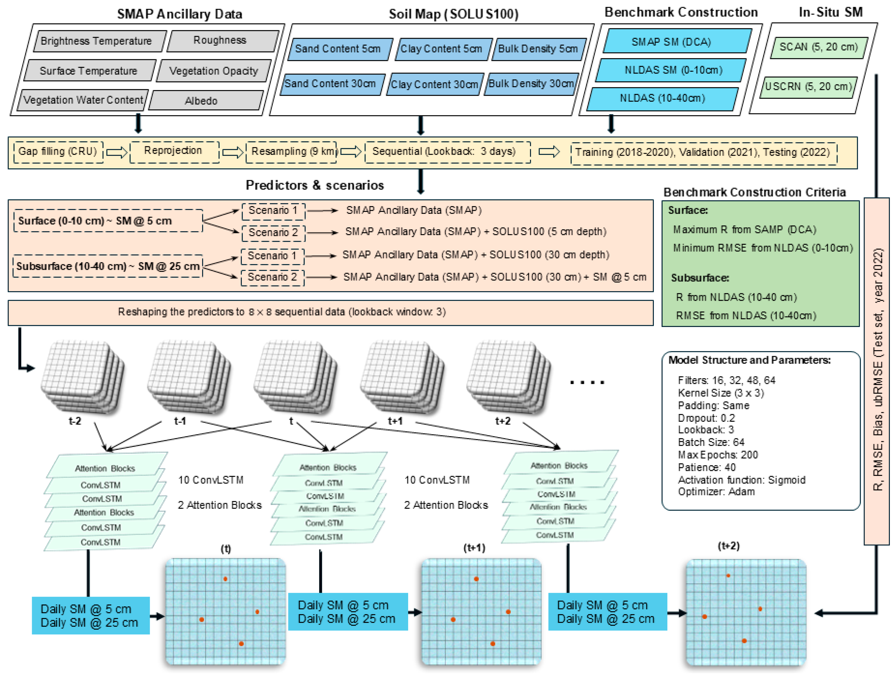
Figure 2.
Spatial distribution of USDA soil textural classes for surface layer (0-10 cm) produced by SOLUS100 maps along with the location of SCAN and USCRN soil moisture networks across the CONUS.
Figure 2.
Spatial distribution of USDA soil textural classes for surface layer (0-10 cm) produced by SOLUS100 maps along with the location of SCAN and USCRN soil moisture networks across the CONUS.
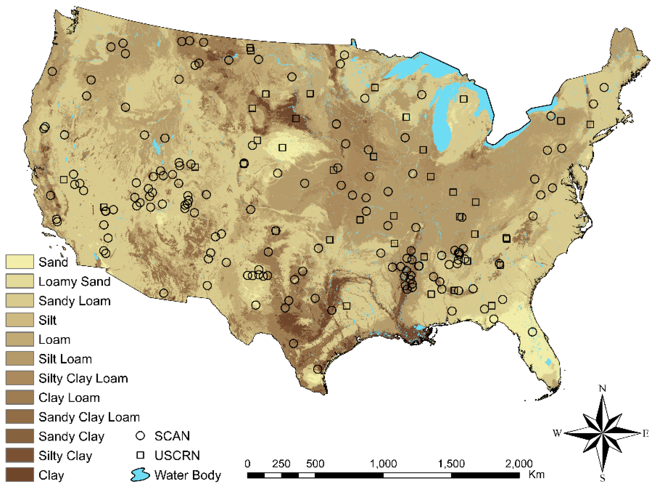
Figure 3.
Error metrics of estimated SM with ConvLSTM against in-situ SM from SCAN and USCRN (all data together) and NLDAS-2 SM for surface (5 cm) and subsurface (25 cm) depths based on scenarios 1 (S1) and 2 (S2) for fine-, medium- and coarse-textured soils (test set).
Figure 3.
Error metrics of estimated SM with ConvLSTM against in-situ SM from SCAN and USCRN (all data together) and NLDAS-2 SM for surface (5 cm) and subsurface (25 cm) depths based on scenarios 1 (S1) and 2 (S2) for fine-, medium- and coarse-textured soils (test set).
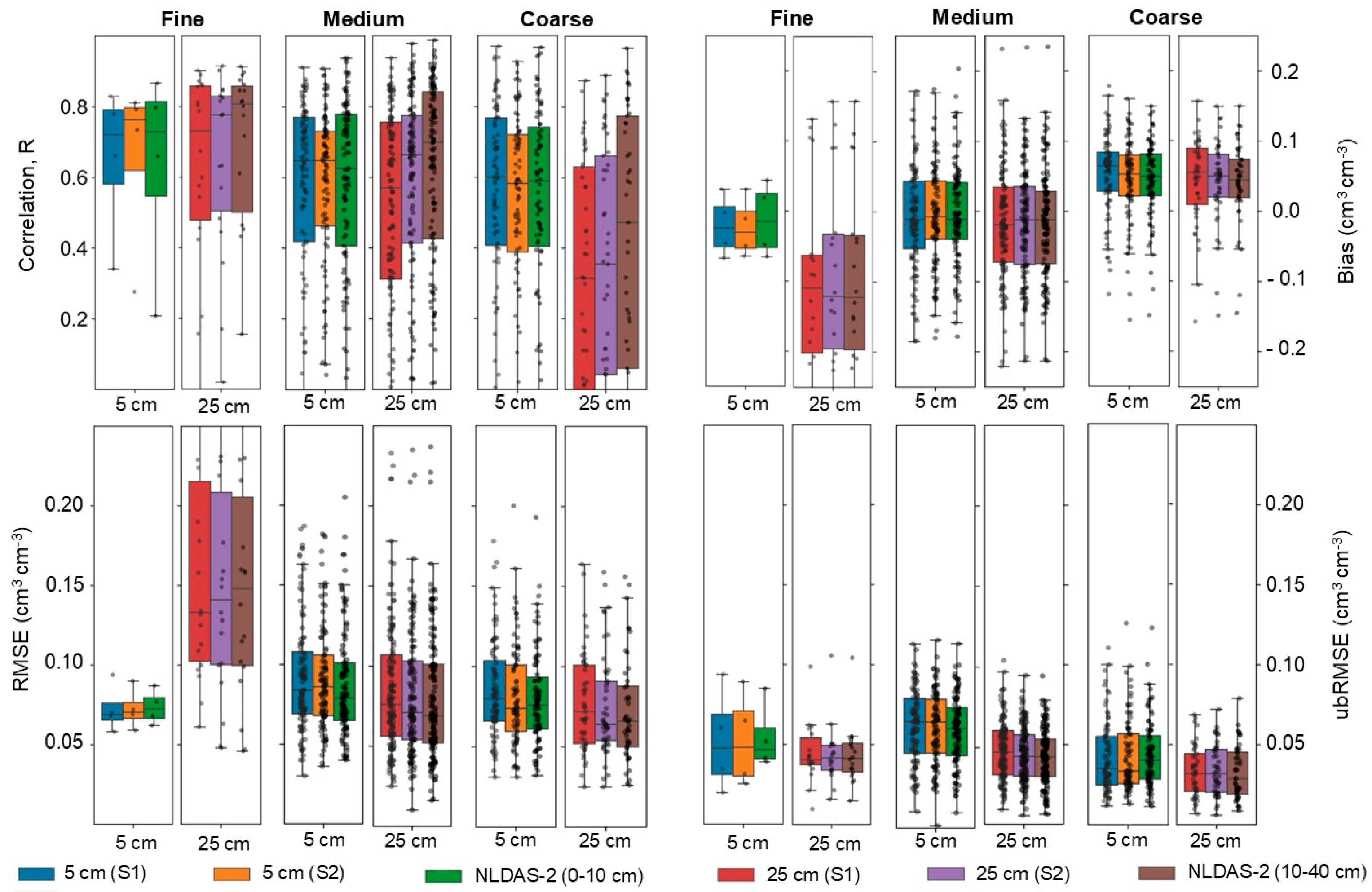
Figure 4.
The error metrics of surface and subsurface SM estimation using the ConvLSTM and scenarios 1 and 2 (S1 and S2) for various land cover types (from MODIS satellite product) against SCAN and USCRN in-situ SM and NLDAS-2 SM products (test set). The land cover type classes include Grassland (G), Cropland (C), Permanent Wetlands (PW), Savannas (S), Open Shrublands and Closed Shrublands (OS/CS), and Woody Savannas (WS). The numbers in parentheses represent the number of soil moisture stations (SCAN and USCRN) in each land cover type.
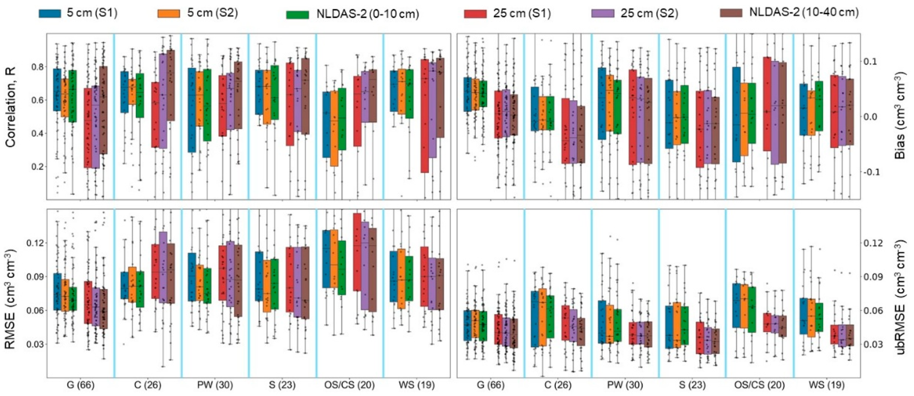
Figure 5.
Error metrics (R, ubRMSE, and Bias) maps of the ConvLSTM-based surface and subsurface SM estimations from scenario 2 (i.e., SMAP ancillary data and SOLUS100 soil properties inputs) against SCAN and USCRN in-situ SM measurements (test set). The vertical lines in the histograms show median.
Figure 5.
Error metrics (R, ubRMSE, and Bias) maps of the ConvLSTM-based surface and subsurface SM estimations from scenario 2 (i.e., SMAP ancillary data and SOLUS100 soil properties inputs) against SCAN and USCRN in-situ SM measurements (test set). The vertical lines in the histograms show median.

Figure 6.
Density scatter plots between ConvLSTM-based surface (5 cm) and subsurface (25 cm) SM estimation (scenario 2) and SCAN and USCRN in-situ SM measurements.
Figure 6.
Density scatter plots between ConvLSTM-based surface (5 cm) and subsurface (25 cm) SM estimation (scenario 2) and SCAN and USCRN in-situ SM measurements.
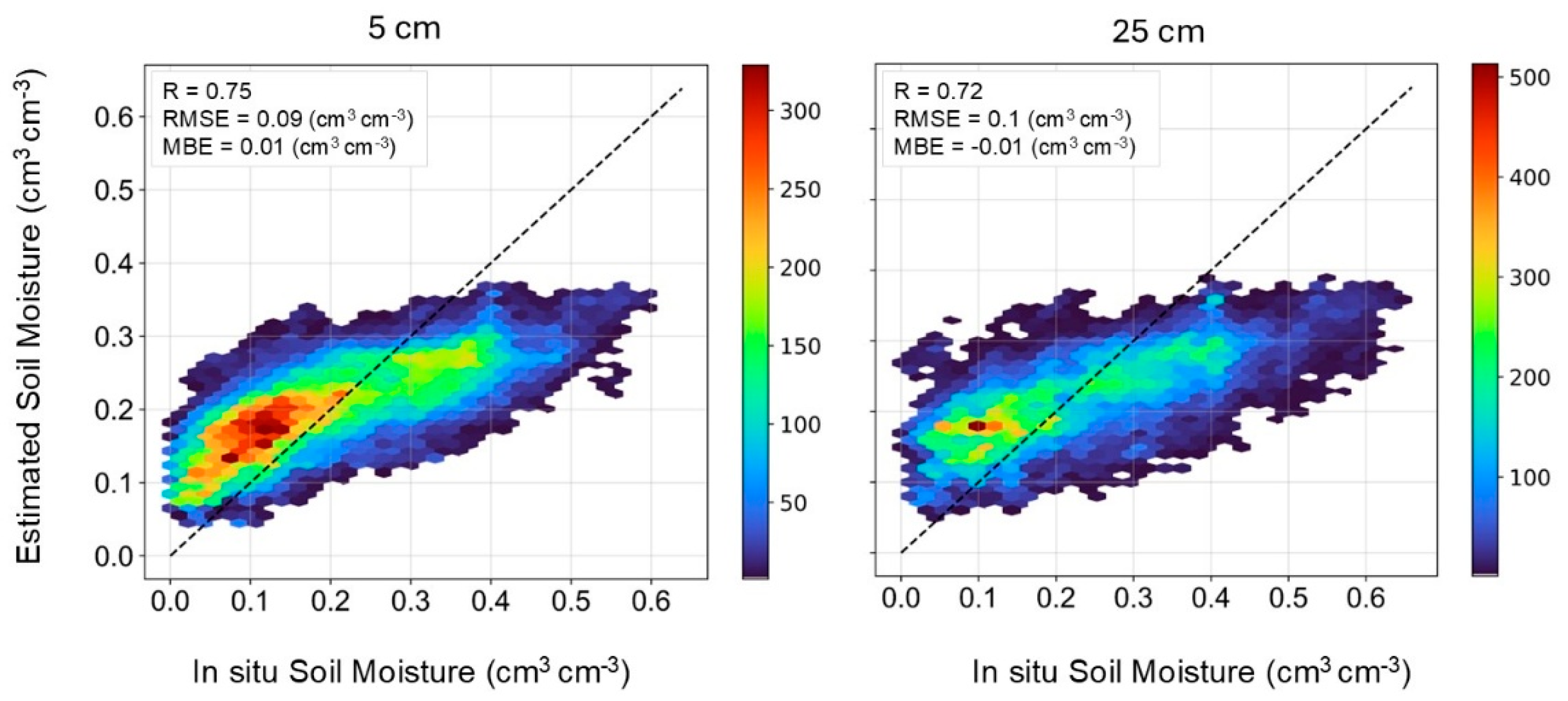
Figure 7.
Temporal dynamics of surface and subsurface SM from the ConvLSTM model (scenarios 1 and 2 and NLDAS-2 against in-situ SM for three SCAN sites (the blue bars depict precipitation) (left); and the associated cumulative distribution function (CDF) curves (right).
Figure 7.
Temporal dynamics of surface and subsurface SM from the ConvLSTM model (scenarios 1 and 2 and NLDAS-2 against in-situ SM for three SCAN sites (the blue bars depict precipitation) (left); and the associated cumulative distribution function (CDF) curves (right).
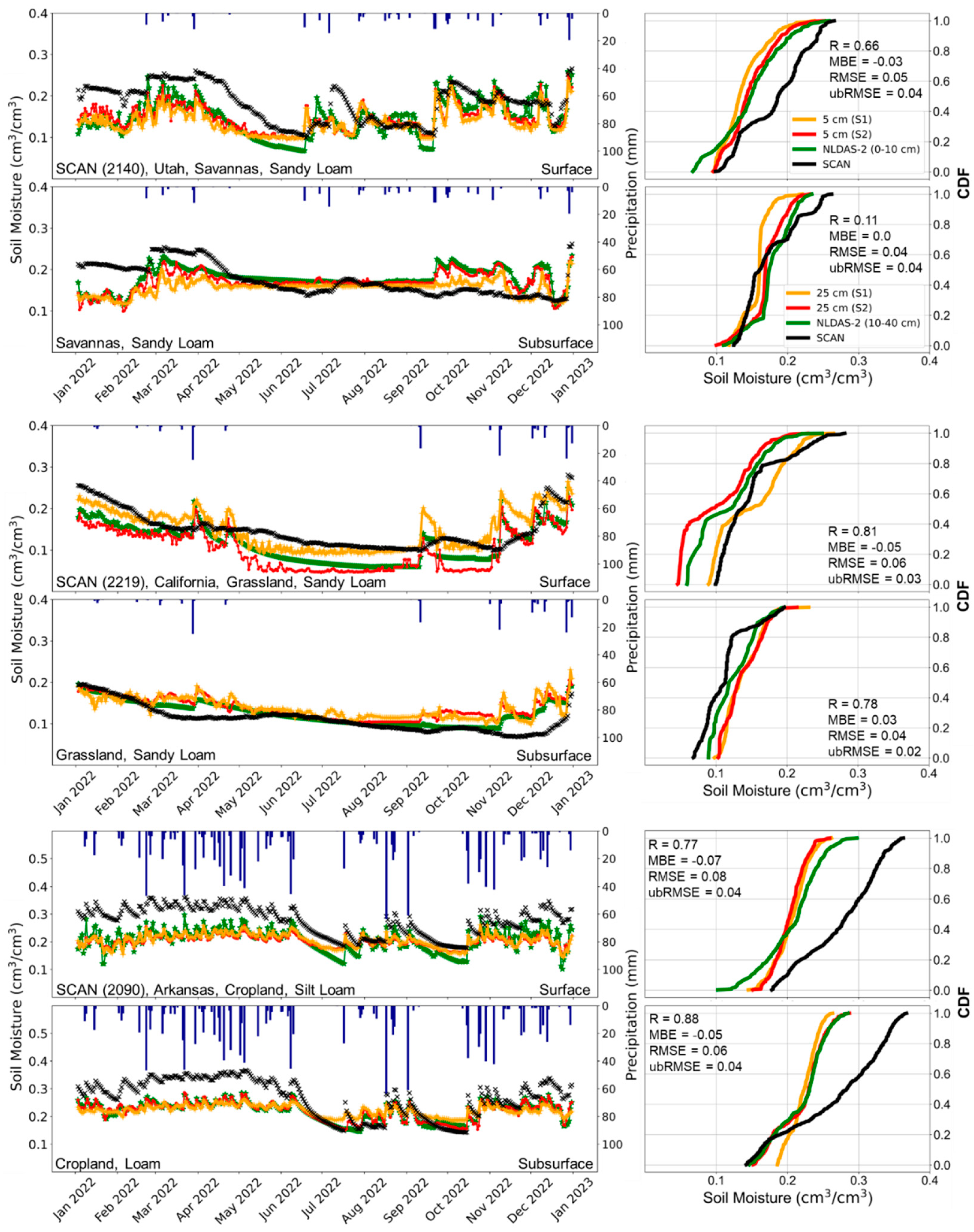

Table 1.
Validation of SM products from SMAP DCA (level 3) and NLDAS-2 over the SCAN and USCRN sites (2018-2022).
Table 1.
Validation of SM products from SMAP DCA (level 3) and NLDAS-2 over the SCAN and USCRN sites (2018-2022).
| Land-cover type | Model | SCAN | USCRN | |||||||
| R | RMSE | Bias | unRMSE | R | RMSE | Bias | unRMSE | |||
| (-) | cm3 cm-3 | (-) | cm3 cm-3 | |||||||
| Grasslands | DCA | 0.63 | 0.070 | 0.008 | 0.057 | 0.69 | 0.079 | -0.02 | 0.050 | |
| NLDAS-2 | 0.65 | 0.073 | 0.031 | 0.053 | 0.60 | 0.070 | 0.014 | 0.049 | ||
| Croplands | DCA | 0.55 | 0.094 | -0.01 | 0.069 | 0.68 | 0.093 | -0.06 | 0.056 | |
| NLDAS-2 | 0.54 | 0.092 | -0.01 | 0.066 | 0.54 | 0.078 | -0.04 | 0.065 | ||
| Permanent Wetlands | DCA | 0.64 | 0.077 | 0.011 | 0.056 | 0.66 | 0.116 | 0.019 | 0.051 | |
| NLDAS-2 | 0.60 | 0.081 | 0.022 | 0.050 | 0.59 | 0.091 | -0.01 | 0.055 | ||
| Woody Savannas | DCA | 0.62 | 0.111 | 0.076 | 0.064 | 0.72 | 0.104 | 0.051 | 0.049 | |
| NLDAS-2 | 0.58 | 0.089 | 0.021 | 0.062 | 0.53 | 0.078 | 0.004 | 0.050 | ||
| Savannas | DCA | 0.66 | 0.085 | 0.020 | 0.054 | 0.78 | 0.098 | 0.069 | 0.045 | |
| NLDAS-2 | 0.64 | 0.086 | 0.017 | 0.053 | 0.65 | 0.078 | 0.015 | 0.044 | ||
| Open and Closed Shrubland | DCA | 0.61 | 0.126 | 0.090 | 0.056 | 0.69 | 0.095 | 0.034 | 0.042 | |
| NLDAS-2 | 0.57 | 0.098 | 0.014 | 0.054 | 0.50 | 0.071 | -0.02 | 0.050 | ||
| R: Pearson correlation; RMSE: Root mean squared error; Bias: Mean bias error; unRMSE: Unbiased RMSE | ||||||||||
Table 2.
Predictors for surface and subsurface SM estimation along with the selection of SM reference data for generating benchmark SM for training the ConvLSTM model [surface: low RMSE of NLDAS-2 SM (0-10 cm) and high R of SMAP DCA SM (5 cm); subsurface: NLDAS-2 SM (10-40 cm)].
Table 2.
Predictors for surface and subsurface SM estimation along with the selection of SM reference data for generating benchmark SM for training the ConvLSTM model [surface: low RMSE of NLDAS-2 SM (0-10 cm) and high R of SMAP DCA SM (5 cm); subsurface: NLDAS-2 SM (10-40 cm)].
| Soil Layer (cm) | Scenarios | Predictors | SMAP SM (DCA) | NLDAS-2 SM | ||
| RMSE | R | RMSE | R | |||
| Surface (5 cm) |
1 | SMAP ancillary data | * | * | ||
| 2 | SMAP ancillary data, SLOUS* | * | * | |||
| Subsurface (25 cm) |
1 | SMAP ancillary data, SOLUS** | * | * | ||
| 2 | SMAP ancillary data, SOLUS**, SM @ 5 cm | * | * | |||
| SOLUS*: Sand, Silt, Clay and Bulk density maps at surface soil layer (5 cm) SOLUS**: Sand, Silt, Clay and Bulk density maps at subsurface soil layer (25 cm) SM @ 5 cm: Estimated soil moisture at depth 5 cm. | ||||||
Table 3.
Mean error metrics indicating the accuracy of ConvLSTM-based surface of subsurface soil moisture estimates for scenarios 1 and 2.
Table 3.
Mean error metrics indicating the accuracy of ConvLSTM-based surface of subsurface soil moisture estimates for scenarios 1 and 2.
| Soil Depth (cm) | Scenario* | R | RMSE (cm3 cm-3) |
Bias (cm3 cm-3) |
ubRMSE (cm3 cm-3) |
| 0 – 10 cm | 1 | 0.54 | 0.089 | 0.017 | 0.053 |
| 2 | 0.54 | 0.086 | 0.016 | 0.053 | |
| 10 – 40 cm | 1 | 0.45 | 0.090 | -0.01 | 0.043 |
| 2 | 0.51 | 0.086 | -0.008 | 0.041 | |
| *Scenario 1: SMAP ancillary data; Scenario 2: SMAP ancillary data and SOLUS100 maps. | |||||
Disclaimer/Publisher’s Note: The statements, opinions and data contained in all publications are solely those of the individual author(s) and contributor(s) and not of MDPI and/or the editor(s). MDPI and/or the editor(s) disclaim responsibility for any injury to people or property resulting from any ideas, methods, instructions or products referred to in the content. |
© 2024 by the authors. Licensee MDPI, Basel, Switzerland. This article is an open access article distributed under the terms and conditions of the Creative Commons Attribution (CC BY) license (http://creativecommons.org/licenses/by/4.0/).
Copyright: This open access article is published under a Creative Commons CC BY 4.0 license, which permit the free download, distribution, and reuse, provided that the author and preprint are cited in any reuse.


