
Submitted:
20 October 2025
Posted:
21 October 2025
You are already at the latest version
Abstract
Accurate root-zone soil moisture prediction is critical for precision irrigation and sustainable crop management, yet it remains challenging due to the complex spatiotemporal interactions between soil and climate. This study presents an optimized hybrid deep learning framework that combines Convolutional Neural Networks (CNN) for feature extraction with Long Short-Term Memory (LSTM) networks for temporal sequence modelling to predict soil moisture across five subsurface layers M1-M5 (5-105 cm) in Malaysian cocoa plantations. A systematic lag optimization revealed that a 7-day lag provides the best balance between complexity and predictive accuracy, enhancing temporal feature learning. To improve transparency, Integrated Gradients (IGs) based attribution analysis was applied to identify the most influential climatic and temporal drivers at varying depths. Robustness was further validated by injecting Gaussian noise (5-20%) into meteorological inputs, showing minimal accuracy degradation. Across all layers and zones, the optimized framework consistently achieved strong predictive performance (R² > 0.94) with low error values (average RMSE ≈ 0.72, MAE ≈ 0.41, MAPE < 3%). These findings demonstrate that hyper-tuned hybrid CNN-LSTM models, when combined with explainable AI and robustness analysis, can deliver reliable and interpretable soil moisture forecasts. The framework provides a practical foundation for data-driven irrigation scheduling and adaptive water management in tropical agro-ecosystems and can be extended to broader agricultural applications.
Keywords:
multi-layer soil moisture
; root zone
; CNN-LSTM
; integrated gradient attribution
; Gaussian noise
; eXplainable AI
; precision agriculture
1. Introduction
The demand for freshwater is escalating globally due to the combined effects of climate change and rapid population growth. Agriculture, being the largest consumer of freshwater, accounts for over 70% of global water usage, primarily for irrigation purposes [1]. Efficient water management in agriculture is therefore critical to ensure sustainable water use while maintaining healthy crop growth. Over-irrigation or under-irrigation can significantly impact plant health and productivity, making the development of accurate and efficient irrigation systems a necessity [2,3]. Precision Agriculture (PA) has emerged as a promising solution to address these challenges by leveraging advanced technologies to optimize irrigation practices. PA integrates information technology, real-time sensing, and data-driven decision-making to crop recommendation and productivity [4], improving water use efficiency, reduce energy consumption, and enhance crop yields [5,6]. This integration helps in predicting and managing crop yields, thereby advancing the overall field of agriculture [7,8].
In terms of cocoa plantation, the moisture content of the soil must be maintained at a constant level to optimally grow and to enable flowering and yielding, indicating that cocoa is highly sensitive to water stress. The ideal rainfall distribution is between 1300 to 2800mm, however south tropics’ rainfall which is largely over 2800mm suffers from irregular distribution resulting in dry spells that necessitate irrigation [9]. The abundance of aluminium and iron oxides in lateritic soil, can be seen through the temperate regions, which further contributes to the moisture retention of soil [10]. Studies often suggest a crop’s daily water needs to be around 3-6mm, while in reality field measurements demonstrate significantly lower rates of evapotranspiration (<2mm/day). Drought is a major culprit due to symptoms such as leaves dropping, photosynthetic activity slowing down, and stomatal closure at leaf water potential below 1.5 MPa [11,12]. Cocoa yield is described to increase with the addition of precise irrigation as Assante et al. found a relative gap in yield of up to 86% [13]. However, this number fluctuates dramatically when considering the interaction of temperature, dry or humid air and ever-changing soil conditions. These parameters are crucial for sustained growth with climate evolutionary shifts, as most cocoa is grown by smallholders who are heavily constrained in irrigation access. In all, irrigation practices alongside effective management of water resources calls for additional research in cocoa production.
Traditional irrigation management systems often rely on statistical models such as regression analysis, fuzzy decision systems, and system identification to predict irrigation needs based on historical data [14]. While these methods have shown some success, they are limited in their ability to handle complex, non-linear relationships in environmental and soil data. In recent years, machine learning (ML) models have gained prominence due to their superior performance in predicting irrigation requirements with fewer data inputs compared to traditional mechanistic models [15,16]. For instance, Support Vector Machines (SVM) and Adaptive Neuro-Fuzzy Inference Systems (ANFIS) have been used to predict soil moisture content using meteorological and crop data. However, these models often struggle to accurately predict soil moisture across multiple layers, limiting their applicability in precision irrigation systems [17,18].
Recent advances in Machine Learning (ML) and deep learning have demonstrated significant improvements in Soil Moisture (SM) prediction for agricultural applications [19]. A study by Dolaptsis et al. [20] developed a hybrid LSTM model for irrigation scheduling in maize crops, integrating soil sensor data, weather station measurements and satellite-derived vegetation indices. To address data limitations, the researchers used the Aquacrop 7.0 model to simulate missing soil moisture content (MC) values, enabling the LSTM to achieve high prediction accuracy with R² values ranging from 0.8163 to 0.9181 for Field 1 and 0.7602 to 0.8417 for Field 2. The model's strong performance highlights its potential for optimizing irrigation in precision agriculture.
Other studies have explored different ML approaches for SM prediction. Nguyen et al. [21] proposed an extreme gradient boosting regression (XGBR) model optimized with a genetic algorithm (GA) that achieved superior accuracy (R² = 0.891, RMSE = 0.875%) compared to other ML techniques when applied to multi-sensor data from Sentinel-1, Sentinel-2, and ALOS DSM. Similarly, Acharya et al. [22] evaluated various ML models for SM prediction in the Red River Valley, finding that random forest regression (RFR) and boosted regression trees (BRT) performed best, with R² values of 0.72 and 0.67, respectively, and RMSE below 0.048 m³/m³. These results underscore the effectiveness of ensemble ML methods in SM estimation.
Deep learning models have also shown promise in capturing complex spatio-temporal SM dynamics. Koné et al. [23] compared LSTM, Bi-LSTM, and a hybrid CNN-LSTM model, with the latter achieving the highest accuracy (R² = 0.9838, RMSE = 0.3672) by leveraging both spatial and temporal dependencies in the data. Similarly, Celik et al. [24] developed an LSTM model integrating Sentinel-1 SAR data, SMAP satellite observations, and climate variables, achieving an R² of 0.87 and RMSE of 0.046. Huang et al. [25] employed a Convolutional LSTM (Conv-LSTM) model that achieved exceptional accuracy (R² = 0.92, MAE = 0.028 m³/m³) while using explainable AI techniques to identify precipitation as the most influential factor. These studies highlight the advantages of deep learning architectures in handling multi-source, high-dimensional SM data. These studies highlight the advantages of deep learning architectures in handling multi-source, high-dimensional SM data.
Innovative approaches combining physical models with ML have further enhanced SM predictions. Lü et al. [26] introduced a CNN-LSTM-Attention (CLA) model that incorporated Hydrus-1D simulations and MODIS vegetation parameters, significantly outperforming traditional LSTM and CNN-LSTM models with an R² of 0.9298 at deeper soil layers. Geng et al. [27] proposed physically-guided LSTM networks (PHY-LSTM) that integrated water balance principles into the loss function, improving SM forecasts by 20.7% in R² compared to standard LSTM. Datta and Faroughi [28] developed a novel multi-head LSTM ensemble that achieved 95.04% R² for monthly SM predictions, addressing the challenge of long-term forecasting accuracy. These hybrid approaches demonstrate how domain knowledge can be effectively combined with data-driven methods for more robust SM modelling. These hybrid approaches demonstrate how domain knowledge can be effectively combined with data-driven methods for more robust SM modelling.
The application of ML for SM prediction has also been explored in specific cropping systems. Dubois et al. [29] tested neural networks (NN), random forests (RF), and support vector regression (SVR) for short-term SM forecasting in potato farming, with NN achieving R² scores above 0.92 for one-day-ahead predictions. Kisekka et al. [30] compared ML and semi-empirical models for root zone SM (RZSM) prediction in vineyards, finding that random forest (RF) outperformed pySEBAL and EFSOIL models with an R² of 0.85 and RMSE between 0.012 and 0.036 cm³/cm³. A et al. [31] demonstrated that RF models could achieve R² of 0.84 for RZSM prediction when trained with sufficient data (70-80% of dataset), outperforming traditional semi-empirical approaches. These crop-specific studies illustrate the versatility of ML in addressing diverse agricultural water management challenges. These crop-specific studies illustrate the versatility of ML in addressing diverse agricultural water management challenges.
Remote sensing data fusion has emerged as a powerful tool for large-scale SM monitoring. Zhao et al. [32] developed an LSTM-based framework to integrate SMAP, AMSR2, and ASCAT satellite data, achieving a median unbiased RMSE (ubRMSE) of 0.052 cm³/cm³ and Pearson correlation (R) of 0.77, outperforming traditional Triple Collocation methods. Wu et al. [33] evaluated multi-modal UAV data (RGB, multispectral, thermal) for SM prediction in citrus orchards, with a hybrid CNN-LSTM model achieving the best results (R² = 0.80–0.88). These approaches demonstrate the potential of combining ML with remote sensing for high-resolution SM mapping.
The recent research has shown that ML and deep learning models can significantly improve SM prediction accuracy across various crops and scales. Hybrid approaches that combine physical models with data-driven techniques, along with multi-source data fusion, appear particularly promising for advancing precision irrigation and water management in agriculture. The consistent performance of LSTM-based architectures (R² > 0.8 in most studies) highlights their suitability for modelling the complex temporal dynamics of soil moisture. Future work could focus on enhancing model interpretability and expanding these methods to additional crops and regions to further support sustainable water use in agriculture.
Recent years have seen significant progress in applying machine learning (ML) and deep learning techniques to soil moisture (SM) prediction, though important challenges remain. These methods show particular promise for precision irrigation applications, but their effectiveness depends heavily on data quality, model architecture, and specific agricultural contexts. While ML and deep learning models have demonstrated strong performance in soil moisture prediction, several limitations remain. A key challenge is the dependency on high-quality, continuous input data, as seen in the work by Dolaptsis et al. [20], where missing sensor data required supplementation from Aquacrop simulations. Many studies like those of Nguyen et al. [21] and Celik et al. [24] rely on satellite or UAV data that may be affected by cloud cover or temporal resolution constraints. Additionally, most models show variable performance across different soil types, crops and climate conditions, as noted in vineyard versus maize applications, suggesting limited generalizability[30] [20]. The computational demands of deep learning approaches may also hinder real-time implementation in resource-constrained agricultural settings. Future research should address these limitations through improved data collection methods, hybrid modelling approaches, and development of more efficient algorithms suitable for edge computing in field applications.
To address these limitations, this study proposes a novel approach that combines Convolutional Neural Networks (CNN) for feature extraction with a hybrid Gated Recurrent Unit (GRU) and Long Short-Term Memory (LSTM) algorithm for soil moisture prediction. CNNs are highly effective in extracting spatial features from complex datasets, making them suitable for processing environmental and soil data [34,35,36,37]. On the other hand, GRU and LSTM networks excel at capturing temporal dependencies in time-series data, which is crucial for accurate soil moisture prediction [38,39,40]. By integrating these two architectures, the proposed model aims to improve the accuracy of multi-layer soil moisture predictions, enabling more precise and efficient irrigation management. This approach leverages seven environmental features and five layers of soil moisture data to develop a robust prediction system that can be integrated into precision agriculture frameworks. Wang et al. [38], in 2024, conducted a study on multiple network structures in order to predict moisture contents in soil and found LSTM to be especially suited for the task. They collected data from multiple depth layers and concluded hybrid models of LSTM like FA-LSTM and GAN-LSTM to be the best performers.
The proposed model represents a significant advancement in precision irrigation by combining the strengths of CNNs for feature extraction and GRU-LSTM for temporal modelling. This hybrid approach not only enhances prediction accuracy but also provides a scalable solution for real-time irrigation management. By addressing the limitations of existing models, this study contributes to the development of sustainable agricultural practices that optimize water use, reduce energy consumption, and improve crop productivity.
2. Study Area, Probe Deployment and Data Collection
In this section, the study area characteristics, sensor deployment strategy and data collection procedures are briefly outlined. The focus is on capturing multi-layer soil moisture variability in a cocoa plantation using strategically placed probes, ensuring comprehensive coverage for effective model training and evaluation.
2.1. Study Area
The soil moisture prediction study was carried out in Bagan Datuk, Perak, Malaysia, (N 3.53°~ N 3.54°, E 100.51°~100.52° E). The map of the research region has been shown in Figure 1. This region has a continually hot and rainy humid climate all year round. The period from October to March, the Monsoon season in Northeast and the period from April to September, the Southwest Monsoon; creates a particularly high humidity climate in Malaysia [41]. The study area, Perak, Malaysia, faces the Northeast Monsoon and tends to have a little more rainfall and affects soil moisture content.
The texture of the soil determines factors such as the retention of water, absorption capacity and infiltration rates of the soil. In the studied region, surface soil (up to 25 cm depth) has sandy loam in the upper layer but clay loam and clay rock deeper down. Data on the moisture of the soil verified that the deepest sensor (sensor 5 or M5) located at 105 cm registered moisture over 93%, indicating composition of sandy clay.
2.2. Sensor Calibration and Probe Deployment
The study area was divided into three cocoa plantation zones (Zone 1: 1.16 acres; Zone 2: 1.10 acres; Zone 3: 1.13 acres) to capture spatial variability in soil moisture as represented in Figure 2. Zone 1 featured moderately undulating terrain, while Zones 2 and 3 were flatter, representing typical micro-topographical differences in Perak, Malaysia.
Prior to deployment, soil moisture sensors were calibrated on-site to ensure accuracy across soil textures. Soil samples collected at multiple depths were oven-dried to determine true Volumetric Water Content (VWC), which was correlated with sensor readings to derive the regression function:
VWC = 0.660 × Sensor – 15.15, (R² = 0.957)
This calibration enabled reliable conversion of raw sensor values into volumetric water content (m³/m³), minimizing bias and improving data consistency for model training.
Each zone contained six IoT-enabled probes arranged in a star configuration, with five placed radially around a central probe to capture spatial variability efficiently. Each 105 cm probe housed five sensors at depths of 5 cm, 30 cm, 55 cm, 80 cm, and 105 cm, covering the cocoa root zone as depicted in Figure 3. The probes included a data logger, wireless telemetry, and solar power to support continuous 30-minute interval measurements and real-time cloud transmission.Cocoa root systems develop mostly in the top 80 cm to 1.5 meter of soil depth, where nutrition and moisture availability are crucial for optimum development in Malaysia's tropical climate [42]. This rooting pattern requires thorough monitoring and control of soil moisture within the rhizosphere zone to maintain plant health, particularly during dry periods or irregular rainfall events. Irrigation was applied twice weekly during the dry season and once weekly during the monsoon when rainfall was insufficient. Real-time soil moisture visualization via a mobile dashboard enabled continuous field monitoring. This calibrated, multi-layer dataset provided high-resolution, reliable input for the CNN-LSTM model, ensuring reduced sensor noise and improved predictive stability.
2.3. Data Acquisition and Preparation
The Soil moisture and environmental data were collected from the three plantation zones using the calibrated IoT-enabled probes described in Section 2.2. Each probe measured soil moisture at five depths (5, 30, 55, 80, and 105 cm) every 30 minutes, forming a high-resolution multivariate time series. Meteorological variables such as solar irradiance, relative humidity, air temperature, rainfall, wind speed, wind gust, and dew point were recorded concurrently.
Zone 1, monitored for over a year, was used for model training (90%) and validation (10%), while data from Zones 2 and 3 (about 1,300 samples each) were reserved for testing to assess spatial generalization. Data were transmitted in real time to a cloud platform for storage and visualization. Measurements from six probes per zone were averaged to reduce random noise, and missing or faulty readings were corrected through linear interpolation.
The resulting synchronized, multi-layer dataset provided high-quality inputs for deep learning-based spatiotemporal modelling. These processed data were then used for feature extraction and temporal variable construction described in Section 3.
3. Materials and Methods
This part explains the step-by-step approach taken in this research regarding the prediction of soil moisture content using soil sensor data and other related environmental factors. The approach involves data collection, data cleaning and preparation, feature extraction, model architecture, model training, and model testing and evaluation. It was aimed at developing a model that is accurate, generalized and robust enough to predict multi-layer soil moisture in cocoa root zone.
3.1. Feature Engineering
Feature engineering is very important in time-series forecasting because it enables the model to capture and utilize temporal patterns present in the data. In our case, we created several features related to time of the year in order to enable the model to capture seasonality, cyclic behaviour, and calendar effects.
Several time features were extracted, including the day of the year, which represents the sequential day number within the year, and the day of the month, which captures the specific day within a calendar month. The day of the week was also included, where Monday is represented as 0 and Sunday as 6. Additionally, the week of the year was computed to indicate the week number within the year, while the week of the month was derived by dividing the day by 7 and adding 1.
Further, for more seasonal features, a month feature was added to represent the corresponding month's number, and the quarter feature was computed to group the months into four parts of a year. A simplified season indicator was computed by dividing the month number by 2 and adding 1.
In order for the model to learn periodic features, sine and cosine transformations were performed on the day of the year, week of the year, and month of the year, which are expressed as: 'day_of_year', 'day_of_month', 'day_of_week', 'week_of_year', 'week_of_month', 'month_of_year', 'sin(day)', 'cos(day)', 'sin(week)', 'cos(week)', 'sin(month)', 'cos(month)' and 'quarter_of_year'. Lagging features were added to allow the model to learn from the past as well as to understand the temporal dependencies without long input sequences being necessary.
3.2. Model Architecture
A hybrid deep learning model combining Convolutional Neural Networks (CNNs) and Long Short-Term Memory (LSTM) networks was adopted to capture both spatial and temporal features in multivariate time-series data.
3.2.1. CNN Feature Extraction
CNNs are a kind of deep learning model that is especially built to handle grid-like input, such as images, using spatial hierarchies. Unlike traditional neural networks, developed by (Bengio and Lecun [43] in 1977, CNNs employ convolutional layers to automatically and continually learn spatial characteristics from input data, making them very successful for tasks like image classification, object identification, and feature extraction. Due to the numerical nature of the soil moisture dataset, a one-dimensional Convolutional Neural Network (1D-CNN) was used for feature extraction. This design is especially good at capturing local patterns and temporal relationships in sequential numerical data, which improves the model's ability to learn soil moisture dynamics effectively.
CNN Architecture and Key Components
The architecture of a CNN typically consists of several layers, each serving a specific purpose in extracting and transforming features from the input data [44]. The primary components of a CNN are:
Convolutional Layers
Convolutional layers are the fundamental components of CNNs. They extract spatial information from input data by applying a series of learnable filters (or kernels). Each filter glides across the input data, conducting element-wise multiplication and summing to create a feature pattern. Mathematically, the convolution operation can be expressed as:
Here, I is the input data, K is the filter, and (i,j) is the location in the output feature map. The filters detect local patterns like edges, textures, and forms, which are required for higher-level feature extraction.
Activation Functions
Following the convolution procedure, an activation function is used to add nonlinearity to the model. The most often used activation function in CNNs is the Rectified Linear Unit (ReLU), which is defined as:
ReLU assists the network in learning complicated patterns by letting only positive values to pass through, thereby adding sparsity while lowering computational complexity.
Pooling Layers
Pooling layers are used to down sample feature maps, lowering their spatial dimensions while maintaining the most relevant information. The most popular pooling procedure is max pooling, which chooses the highest value from a window of the feature map:
Pooling reduces computational burden, prevents overfitting, and makes the model more resilient to tiny translations in the input data.
Fully Connected Layers
After multiple convolutional and pooling layers, the collected features are flattened and sent through one or more fully connected layers. These layers integrate information to provide the final output, such as class probabilities in classification tasks.
Dropout
Dropout is a regularization method that helps to avoid overfitting. During training, random neurons are "dropped out" (turned to zero) with a predetermined probability, driving the network to acquire stronger characteristics.
CNN for Feature Extraction
In feature extraction, CNNs are used to learn and extract meaningful characteristics from raw input data. The convolutional layers function as feature detectors, recording hierarchical patterns from low-level features (such as edges and textures) to high-level features [45]. These features may then be fed into other models, such as RNNs or hybrid models, to perform tasks like time series prediction or sequence modelling.
3.2.2. LSTM
Before starting LSTM, it is mandatory to introduce Recurrent Neural Network (RNN) first because LSTM is a variant of RNN. RNN was first introduced in 1980s. RNN are somewhat similar to Forward Feed Neural Networks (FFNN). Only difference is, RNN has self-feedback of neurons in the hidden layers. These structures help RNN to learn past data and enables the RNN to process sequences. That why RNN models are more effective in learning sequences.
The hidden nodes = (,……., ) and output nodes = (,………, ) are calculated by looping over by equations (1) and (2) below:
where xt is the input vector at time t, and ht-1 is the hidden cell state at time t-1, b0 and bh are the bias vector and U, W, V are the weight matrices for input-to-hidden, hidden-to-hidden, and hidden-to-output connections, respectively.
The loss is determined as the total loss at each time step. The gradients are determined using Back Propagation Through Time (BPTT) [46]. However, BPTT is insufficiently efficient to learn a pattern from long-term dependence due to a gradient vanishing issue [47]. To address this issue, Hochreiter and Schmindhuber created LSTM in 1997, which enforces constant error flows using Constant Error Carousels (CEC) inside certain multiplication units [48]. These specialized units manage the error flow by learning how to open and shut certain gates. The memory block of the LSTM is made up of CEC, three special multiplicative, and gate units. The continuous error carousels run throughout the network without an activation function, thus the gradient does not dissipate when BPTT is used to train the LSTM structures. Because information may readily travel across the whole network unmodified, LSTM is more suited to learning long-term knowledge than RNN. Furthermore, the memory block's input, forget, and output gates may govern information flow inside the block. The input, forget, and output gates govern the amount of information that goes into CEC cells, is stored in the cell, and flows out of the cell into the rest of the networks. The architectural diagram below (Figure 4) depicts LSTM memory blocks and their associated components along with CNN framework.
Similar to RNN, the LSTM computes the mapping from an input sequence x to an output sequence y by looping through the equation (3) to (8) with initial values c0 = 0 and h0 = 0.
where Wi, Wf , W0 represent the matrix of weight from the input, forget and output gates to the input respectively and Ui, Uf, U0 denote the matrix of the weights from the input, forget, and output gates to the hidden layer respectively. bi, bf and b0 represent the bias vectors related to the input, forget, and output gates, σ is the element wise nonlinear sigmoid activation function.
it, ft, 0t and ct are the input, forget, output gates and cell state vectors at time t, respectively. The element wise vector multiplication is represented as ⊗.
3.2.3. Proposed 1D-CNN-LSTM Hybrid Model
To accurately capture both short-term and long-term dependencies in time-series data, a hybrid 1D-CNN-LSTM model was designed. This approach is necessary because convolutional layers excel at extracting local patterns, while LSTMs specialize in learning sequential dependencies over time. The architecture of the proposed model has been given in Figure 4.
The model begins with a CNN component that acts as a feature extractor. It consists of four Conv1D layers, each with 64 filters, a kernel size of three, and ReLU activation. These layers detect short-term temporal dependencies by identifying localized patterns in the data. The final convolutional layer feeds into a softmax layer, refining the extracted features before passing them to the LSTM. Following this, five LSTM layers process the sequential data to capture long-term dependencies.
Traditional dropout applied to input connections in LSTM layers provides some regularization, but it is often inadequate for recurrent neural networks, particularly when the goal is to capture long-term temporal correlations within dynamic environments. To overcome this, recurrent dropout has been shown to be more successful at minimizing overfitting by randomly deactivating connections between hidden states over time steps, rather than only between input and hidden layers. This method enhances generalization while retaining LSTMs' memory capacities, which is critical for prediction of soil moisture sequences impacted by previous weather parameters. In this proposed model, each LSTM layer has 50 units with a recurrent dropout of 0.1. This technique proved effective in retaining essential sequence information while avoiding overfitting in noisy or limited dataset which is very common in smart agricultural practices.
The first four LSTM layers return sequences, ensuring that temporal dependencies are maintained across layers, while the final LSTM layer continues processing the learned patterns. The extracted features are then passed to a Dense layer with 128 units and ReLU activation to enhance the representation of the learned information. Finally, a single neuron in the output layer, with linear activation, enables the model to handle regression tasks like predicting soil moisture content. The overall architecture with details of hyper-parameters on the layers has been compiled in Table 1.
By integrating CNN for feature extraction and LSTM for sequential learning, this model effectively captures both localized fluctuations and long-term trends, improving the accuracy of time-series predictions. To guarantee generalizability and reduce overfitting, early stopping was implemented by tracking validation loss. Training was ended when no substantial increase in validation performance was seen after a predetermined number of successive epochs, keeping the model state that produced the best validation results. This method substantially increased model resilience while preventing overfitting to the training data.
3.3. Data Correlation Analysis
The correlation matrices for Zones 1, 2, and 3 show the associations between the environmental parameters and the soil moisture quantities which are crucial for feature selection and accurate soil moisture prediction in root zone for cocoa.
The correlation matrix for zone 1 has been given in Figure 5. Zone 1 shows a strong positive correlation between temperature and solar irradiance (0.86), reflecting their direct relationship. Soil moisture layers M2-M3 also exhibit high correlation (0.97), suggesting similar moisture dynamics. Weak correlations exist between rainfall and wind speed (-0.014) and rainfall-M4 (-0.0097), indicating negligible linear relationships. The strongest negative correlation between temperature and relative humidity confirms the expected inverse relationship. These patterns highlight key environmental interactions while revealing variables with minimal dependence.
The correlation matrix for zone 2 has been given in Figure 6. Zone 2 shows patterns similar to other zones, with strong positive correlations between temperature and solar irradiance (0.85) and between soil moisture layers M2-M3 (0.98) and M3-M5 (0.97). Weak correlations exist for rainfall with wind speed (0.046) and M4 (-0.019), as well as for rainfall and solar irradiance (-0.058), indicating minimal linear relationships. The strongest negative correlation between temperature and humidity is observed in this zone as well.
The correlation matrix for zone 1 has been given in Figure 7. Zone 3 follows similar trends as other zones, with strong positive correlations between temperature and solar irradiance (0.85) and near-perfect alignment in soil moisture layers M4-M5 (0.99) and M3-M4 (0.94). Weak correlations exist between rainfall and wind speed (0.046), rainfall and M4 (-0.024), and solar irradiance and rainfall (-0.058), indicating minimal relationships. The strongest negative correlation between temperature and humidity seems to be consistent for all the zone, as seen from the observed patterns.
This correlation analysis is critical for identifying the most significant predictors, which allows the model to prioritize relevant features and decrease noise in the dataset. Understanding this relationship allows the model to better reflect the underlying physical processes that drive soil moisture variability, thereby enhancing prediction accuracy and generalizability over a wide range of agro-climatic environments.
3.4. Run-Time Complexity Analysis
The evaluation of the performance of the soil moisture prediction model under different hardware configurations are discussed in this section. The various configurations’ training and inference times are evaluated to study the impact of the hardware on model performance at different moisture levels and zones. The setups under analysis are CPU-only and GPU-accelerated ones where both share the CPU (2 vCPUs, Xeon, 2.2GHz), RAM (13GB) and Disk (33-100GB). In the case of the GPU setup, there is the addition of an NVIDIA Tesla T4 GPU which has 16GB of VRAM, which increases the GPU configuration's processing speed.
As the zones and moisture levels change, the number of data points affects the model's training and inference speed. For example, Zone 1 (which has larger data points) tends to take longer to train. In contrast, Zones 2 and 3 train on smaller data sets and show sharper declines in training and IGA bouts, where training in Zone 1 is thirty times longer than even the most extensive training in Zone 2. In very few cases, configurations for Zone 1 and Zone 2 dramatically change training. Comparing configurations across these zones will illustrate how Zone 1 and Zone 3 are representative of the larger regions.
The Table 2 shows the setup comparison for both the GPU and CPU configurations in each zone, while moisture levels (M1 to M5) are considered for Zone 1.
In Zone 1, where the data points are more abundant, the model's training times are significantly greater, lasting between 10 minutes 15 seconds to 10 minutes 30 seconds, while the inference times are 340 ms to 345 ms. Table 2 shows that with the GPU, there is a training time reduction from 2 minutes 15 seconds to 2 minutes 25 seconds, and the greater than 10-minute threshold is dramatically exceeded. This shows the efficacy of a GPU setup, which lowers the time spent on processing by one order of magnitude. Even with the large dataset in Zone, the GPU remains extremely effective with large reductions in training and inference times.
The assessment of the hardware setups within Zone 1 clearly shows the performance dividend accruable to the GPU, especially with respect to the reduction of training and inference times. Th training benefits the most from the GPU because of how much the processing times are slashed. In Zones 2 and 3, with smaller data, the training and IGA times drop to 1/3 of the CPU times, with slight differences due to different moisture levels. This illustrates how easily the model can scale to larger regions as the GPU can increase the data sizes with minimal increase in training time. These results augment the model’s real-time predictive capabilities on soil moisture at different points within the cocoa plantations, as compared to other models.
3.5. Evaluation Metrics
Use of evaluation metrics is crucial in analysing the predictive power of a given model. A brief description and analysis of five most popular metrics used in this time-series regression study follows: Mean Squared Error (MSE), Root Mean Squared Error (RMSE), Mean Absolute Error (MAE), Mean Absolute Percentage Error (MAPE) and Coefficient of Determination (R²).
Mean Squared Error (MSE)
An MSE evaluation yields the estimated value once the errors are squared and averaged. Because squaring each error tends to overemphasize its regressive properties, it is sensitive to outliers. MSE is extensively utilized in regression tasks.
Root Mean Squared Error (RMSE)
By its nature, RMSE is the square root of MSE, and shows the average magnitude of a set of values relative to the variable of interest. For the purpose of interpretation, it is greatly preferred over MSE and even MAPE, which is why it remains popular for regression models.
Mean Absolute Error (MAE)
As MAE is used to assess the average of all absolute predicted values, it can only be positive or zero. Despite MAE being more lenient on MAE, it is more comprehensible than MSE due to the lack of nonlinear squaring.
Mean Absolute Percentage Error (MAPE)
As a metric, MAPE showcases average values of predicted and real values that are useful for estimation. This measure does allow for greater accuracy relative to the prediction values when actual values differ substantially.
Coefficient of Determination (R²)
R² exists within the range of 0 and 1, where 0 indicates no explanatory power, and 1 indicates a perfect fit. It measures the portion of variance in a dependent variable that can be predicted using the independent variables.
Here, is actual value of the target variable for the i-th data point, is predicted value of the target variable for the i-th data point, is mean of the actual values of the target variable and n is total number of data points in the dataset. These metrics are widely employed in assessing the effectiveness of a model in completion of regression tasks. Each and every regression metric comes with its set of pros and cons, and the issue at hand determines which metric is best suited for a given task.
3.6. Noise Injection for Uncertainty Analysis
The proposed model employs multiple meteorological variables in a multivariate time series to capture their influence on soil moisture dynamics. However, atmospheric variability, sensor inaccuracies, and forecasting uncertainties can introduce noise into these inputs, potentially degrading model performance in real-world conditions.
Following [49], adding controlled noise to the test data was found to serve as a convenient proxy for probing a model’s robustness and generalization ability. Performance fluctuation of metrics on noisy conditions enables the measure of sensitivity of the model to perturbations of its input. This variance is really nothing but the use of the model's robustness to perturbations in having the model behave in a real world, uncertain environment in a manner we understand and control.
To evaluate how our model would behave in this kind of setting, we have developed a controlled additive noise scenario. In essence, Gaussian distributed noise was added at the levels of input of 5%, 10%, 15% and 20% in the weather features at source. The goal here is to indicate realistic sensor inaccuracies, absence of data acquisition and a wide variety of oscillation in prediction by means of possible deflection. We can see the trends achieved by the model at each step of noise level increase, so that we can evaluate the degree of sensitivity of the model to the corrupted data and see the limit which the predictor tolerates until we impact drastically in the prediction result.
z = the random variable (feature value after noise injection).
μ = the mean (expected value) of the distribution.
σ = the standard deviation, which controls the spread (how wide or narrow the distribution is).
σ2 = the variance (square of the standard deviation), which measures the dispersion of the distribution.
p(z) = the probability density of observing the value under this Gaussian distribution.
The sensitivity analysis, or robustness analysis, plays mainly two roles. It assists in measuring the degree of uncertainty in the model, which then helps to decide how confidently the model can be trusted, to predict an outcome when it is wrong under such data impoverished and data uncertain conditions. It also points out the robustness of the model, which is highly necessary for practical application particularly for highly sensitive prediction tasks, as it describes the operational error of the model capable of rendering drastic consequences.
4. Results and Analysis
This section uncovers the results of the study step by step and provides a thorough zone wise interpretation. This section meticulously provides the study's findings, providing a complete, step-by-step examination. The emphasis is on a zone-wise interpretation to emphasize spatial diversity within the research region. Each zone's predictive performance is rigorously investigated in terms of model accuracy, error metrics, and soil moisture behaviour, allowing a more nuanced understanding of the model's success in capturing local variation.
4.1. Results of Zone 1
For Zone one, a probe was used to collect moisture from the five layers of the soil. To enable accurate predictions, long term dependencies and spatial patterns were captured using a hybrid LSTM-CNN architecture. The model was trained using a 90-10 split for training and validation. Lag values had been used in batches of 1,3,5,7 and 9 respectively. In time-series prediction, particularly for soil moisture prediction, lag values represent the past observations used as input features to predict future states. Selecting appropriate lags is essential to capture the temporal dependencies and memory characteristics of the soil moisture dynamics across different depths (layers). Using multiple lag intervals enriches the feature set and increases the model's ability to recognize non-linear temporal correlations between layers. Figure 8 shows the heatmap of lag values vs layers of soil in terms of R2.
As per the Figure 8, the predictive accuracy was seen to have a positive correlation with the Lag values. The results that lag 7 showed were mostly superior, while Lag 9 showed little to no margins of improvement and hence, for optimality and reducing complexity, lag 7 was used for our main model.
Following this, plots were evaluated to visualize the accuracy. Figure 9, shows the LSTM-CNN model performance and the actual vs predicted soil moisture values during the five layers in Zone 1. Each subplot corresponds to a specific soil layer, where blue indicates true moisture values, while orange shows the model estimates
The patterns show that the model reasonably simulates moisture oscillations considering all layers, although some differences are still observed. In particular, there are sharp changes in moisture in some high-variability regions that are not perfectly captured. The M4 and M5 layers are less variable, which implies moisture changes in the deeper layers are slower and easier to anticipate. The findings emphasize the capability of the model to capture temporal dependencies and spatial relationships that exist in soil moisture prediction.
Figure 10 scatter plots displays the relationship between predicted moisture values and true value for the five layers of soil in Zone 1. Each smaller plot corresponds to each soil layer from M1 to M5 and shows how model's fit to the data.
The data points in all five layers are almost perfectly aligned with the diagonal dashed line, showing a high relationship between the predicted and true values. In some areas, however, there is a discernible amount of shifting and spreading which points towards some degree of error in predictions. For topsoil (M1), The scatter plots exhibited minimal dispersion, indicating very high accuracy in the prediction of surface moisture. This result is consistent with the results in Table 3, with R² values reported in this layer (above 0.9728 for Zone 1), suggesting reliable model performance near the soil surface where environmental fluctuations are more immediately reflected.
Table 3, exerted the excellent results obtained by the model, with average R² of 0.97. The model performed exceptionally well when evaluated in terms of other metrics like MSE, RMSE, MAE and MAPE, as well. The intermediate layer (M2-M3) scatter plots also showed tight clustering around the diagonal line, with slightly wider dispersion compared to M1. This indicates slightly reduced accuracy as the depth increases, which is expected due to the time lag and buffering effects associated with moisture movement in the soil profile. The deeper soil layers (M4 and M5) seem to show more clustering along the diagonal which suggest these layers had more accurate predictions than the upper layers. This plot is useful to gauge the accuracy of the model to estimate the soil moisture content at various depths within the soil profile.
4.2. Results of Zone 2 and Zone 3
The Hybrid LSTM-CNN Model was trained and tested in Zone 1 to predict soil moisture contents and to further validate its effectiveness and generalization capability, the model was implemented using the complete dataset from Zone 2 and Zone 3. Figure 11 shows the R2 heatmap results of the test across all the five layers, M1 to M5, for different Lag values, Lag 1 to Lag 9.
For Zone 2, Lag 7 also consistently produced high correlation values across all machines, indicating strong predictive potential. While Lag 9 yielded slightly higher values, the improvements were marginal. To balance performance and model simplicity, Lag 7 was selected as the optimal lag for this zone. Lag 7 again emerged as a reliable choice with high values across machines for Zone 3. Although some variability was noted, especially in M4 and M5 at lower lags, Lag 7 offered a good trade-off between accuracy and computational efficiency. Thus, it was chosen as the optimal lag for Zone 3 as well.
To further analyse the performance of the model, the Figure 12 and Figure 13 shows the actual and predicted differences of moisture content for all five soil layers in the two zones with Zone 2 and Zone, respectively.
In both areas, the model retains its robust degree of moisture prediction accuracy, as seen in the results. There is greater stability in moisture retention, resulting in deeper layers having smoother trends. These results validate the model's cross-regional generalizability while underscoring the model's need to better capture sudden changes in surface moisture.
To further assess the model’s predictive accuracy, scatter plots were generated for all five soil layers in Zone 2 and Zone 3 which are presented in Figure 14 and Figure 15, respectively.
The results in the Table 4 and Table 5 shows the strength of the proposed LSTM-CNN model in accurately predicting the moisture level across the zones and across the different depths. The average R² values of over 0.94 for both the zones, highlight the effectiveness of the models in the domain.
Across all layers and both zones, the scatter plots, in Figure 14 and Figure 15, showed a strong linear connection between observed and predicted values, which was almost identical to the dotted diagonal line. This alignment indicates that the model accurately captured the time patterns and magnitudes of soil moisture fluctuations. The near-perfect alignment of the predicted values with observed measurements indicates the model’s strong learning capacity in capturing the complex temporal dynamics of soil moisture under varying field conditions.
4.3. eXplainable AI (XAI): IGA Insights Across All 5 Soil Moisture Layers
Deep learning models like CNN-LSTM are often criticized as “black boxes,” making it difficult to understand how predictions are generated. Integrated Gradients Attribution (IGA) is a powerful XAI technique that assigns importance scores to input features by tracing their contribution from a baseline to the final prediction. This makes IGA particularly valuable for soil moisture prediction, as it reveals which environmental and temporal variables most strongly influence the model across different soil depths. By highlighting these drivers, IGA not only builds trust in the model but also supports smarter, data-driven irrigation decisions. The following section presents IGA-based feature attribution results for all five soil moisture layers (M1-M5).
The heatmaps give an indication of the importance of various features throughout the duration for every moisture level, thus illustrating the features, in the context of their time lags, which most influence the model’s predictions. The Figures in the following pages show results for Moisture Level 1 (M1) through Moisture Level 5 (M5). Each of these illustrates the importance of features such as Humidity, Temperature, as well as the Time features (the Day of the Week, the Month of the Year) for the time lags between t-7 and t-1.
The level 1 moisture (M1) dew point and humidity features, as represented in Figure 16, in the heatmap models demonstrates their pivotal roles in the framework of model predictions with correlation of 0.828 and 0.77 at t-1, respectively. In particular, the attribution values for these features become greater as the time lags move towards t-1. Time features, like the sin(Day) component of Time, tend to demonstrate certain levels of attribution over time lags, which indicates the model’s reliance over these systems. The closer the model is to the point of prediction, the more likely the features of Dew point and Humidity become the paramount factors of consideration.
As shown in Figure 17, the influence of Humidity remains strong at 0.759 at t-1, as the moisture level rises to Moisture Level 2, or M2. However, other features like Wind Gust and Week of Year show more attribution. The model shows increasing sensitivity to temporal patterns with features like sin(Day) and Week of Year becoming more influential in the model’s predictions. More at the later time lags (t-1) the attribution for Dew Point increases, emphasizing its importance as the prediction time gets closer. M2 is a change which suggests the model is starting to incorporate both seasonal and short-term weather patterns in its decision-making.
As shown in Figure 18. the features for Moisture Level 3, or M3, show more pronounced attributions to the seasonal cycle. Dew Point and Humidity remain the most influential features with 0.771 and 0.831 correlative coefficients, especially at the lag t-1, alongside sin(Month) and Wind Speed which now have more impact. The heatmap suggests a more complicated relationship between time of year and the surrounding weather. As lags converge toward t-1, the model’s attributions show greater emphasis on monthly cycles, which suggests that the model’s long-term predictions have incorporated monthly cycles alongside daily features, as well as increasing monthly weather variations, yielding long-term predictions.
There is noticeable change in feature importance at Moisture Level 4 as captured in Figure 19. Although most predicted values appear modest in importance, features associated with time like sin(Month) and Week of Year, as well as weather features like Humidity and Solar Irradiance, begin to dominate the model. At t-1, the values for cos(Day), sin(Month) and Week of month have coefficients of 0.568, 0.569 and 0.523, respectively, indicating the model is being sensitive to seasonality and weather more than before. The increase in Humidity at t-1 along with sin(Month) attribute also suggest that these long-term features are retention more critical than other interval features. The increase in humidity at the time lag and Moisture Level suggest more critical than other interval features.
The model at Moisture Level 5 mirrors long-season cycles and critical weather patterns, with the attributions in Figure 20 more than likely representing the aggregate result of these features. Marked values in Humidity, Week of Month and sin(Month) with coefficients of 0.772, 0.524 and 0.521 at t-1, suggest the model is allocating more attention to these features as the predicted time approaches. At t-1, the attribution for Moisture Level 5 is high compared to other features, meaning the model is dependent and uses the feature to ‘update’ its prediction the most. the increase is retained and ‘stored.’ Like previous moisture levels, M5 exposes long and short weather cycles shifted modelled are driven more than before.
Based on the figures, the evolution in importance of the various features across moisture levels underscores the impact of certain weather elements and climate dynamics on the prediction of soil moisture for cocoa plantations throughout the moisture levels of the plantation. For the lower moisture levels (M1 and M2), elements such as Humidity and the daily cycles dominate in the prediction of short-term moisture changes. For the higher moisture levels (M3 to M5), seasonal and larger scale influences such as Wind Gusts, Solar Irradiance and the time-of-year gain prominence. This investigation enriches the moisture prediction system by elucidating the role of various weather features at different moisture levels. This capability, alongside others, enhances model hyperparameter tuning, to moisture level prediction, to refine predictions on hydraulic control system in the plantation.
4.4. Uncertainty Analysis
This section analyses the level of impact brought about by noise to the quantitative performance of the model across different moisture levels. The included Table 6 shows the influence of different noise levels (0% to 20%) on the MSE, RMSE, MAE and R² metrics across Zone 1.
The model shows excellent results regarding all the moisture levels (M1 to M5) relative to Zone 1. The high R² values seem to hold up even when subjected to higher levels of noise. At zero percent noise, the R² values hold at and above 0.9 indicating excellent predictive accuracy. As noise increases, R² values drop slightly but the model remains resilient. Moisture Level 4 shows the least sensitivity to noise R² down from 0.9573 to 0.9089 at twenty percent noise. Moisture Level 5 shows the most sensitivity, R² dropping from 0.9462 to 0.8679. Moisture Levels 2 and 3 show moderate sensitivity R² values above 0.9 at higher noise levels. Overall performance of the model seems to demonstrate the most noise, while lower levels of moisture seem to demonstrate model robustness with regards to reliable predictions noise environmental conditions.
To assist with further analysis, the model’s predictive outcome has been plotted to better visualize the effects of addition of noise. Figure 21 clearly illustrates the predicted moisture for all the zones across all the moisture levels.
Figure 21 illustrates the model’s prediction performance for Zone 1 across different moisture levels (M1 to M5) under varying noise conditions (0%, 5%, 10%, 15% and 20%). As portrayed in the plots, the model predicts accurately and with stability for M1 and M2 moisture levels, even in the presence of 20% noise. Their predicted values remain in close correspondence with the actual moisture values. For M3, M4, and M5, the moisture levels are too high, which results in model accuracy predicted values and actual values diverging slightly with high levels of noise. The model, however, does remain stable and robust, showing strong predictive capability, even when the conditions are adverse.
Overall, the results highlight the model’s robustness across varying moisture levels and noise conditions. At lower moisture layers (M1 and M2), the model remains relatively stable and resilient to noise, while at higher moisture layers (M3, M4 and M5), its accuracy begins to decline a little. Even under higher noise conditions, the model still maintains relatively strong R² values, reflecting its overall robustness in a variety of scenarios.
5. Discussions
This study evaluates the performance of a hybrid CNN-LSTM model for predicting soil moisture content at five distinct depth layers at rhizosphere (M1 to M5) across three spatially distributed zones within a cocoa plantation in Perak, Malaysia. The overall study of model performance across scatter plots and actual vs predicted time-series graphs verifies the proposed hybrid CNN-LSTM framework's excellent predictive accuracy and resilience for multi-layer soil moisture prediction. The time-series plots demonstrated high temporal coherence, where the model successfully tracked both rapid and gradual changes in soil moisture over time. The surface layer (M1) consistently exhibited the highest accuracy, reflecting the model’s sensitivity to rapid surface moisture changes, while deeper layers (M4 and M5) showed slightly dampened responses which is consistent with known subsurface water dynamics. Similarly, the scatter plots revealed an exceptionally strong correlation between observed and predicted values across all soil layers and all 3 spatial zones, with most points closely aligning along the diagonal line. The evaluation metrics (MSE, RMSE, MAE, MAPE and R²) for best lag value (Lag7) across all the layers in all 3 zone has been given in Table 7.
At the shallowest depth (Topsoil layer M1), the model demonstrated outstanding predictive capacity across all three zones, with R² values of 0.9728, 0.9725 and 0.9572, respectively. RMSE values remained below 0.9 in all zones, with Zone 2 having the lowest value (0.5146). The model correctly described soil moisture fluctuation near the surface, where rainfall and evapotranspiration had a greater impact (average R² = 0.9675). The second layer (M2) performance decreased somewhat, with an average R² of 0.9503, especially in Zone 3, where RMSE was 0.9045 and R² was 0.9461. The pattern was similar in M3, with Zone 3 showing the greatest error levels (RMSE = 1.0125, R² = 0.9402). These findings suggest that model performance decreases with soil depth, most likely owing to delayed and dispersed reactions to surface hydrological inputs. Nonetheless, R² values across all zones remained above 0.94, indicating robust model generalization at this level. In the deeper layers (M4 and M5), further decline in performance was observed. The average R² values dropped to 0.9488 and 0.9404, respectively. Particularly for M4 in Zone 3, the RMSE remained high (0.8630) and R² was lowest (0.9321), suggesting increasing uncertainty in the prediction of deep soil moisture dynamics. Interestingly, Zone 1 in M5 achieved an exceptionally high R² of 0.9855, indicating that deep moisture predictions can still be accurate in certain zones, possibly due to more consistent water retention characteristics or soil texture homogeneity. Zone 1 consistently achieved the highest prediction accuracies across most layers, with R² values above 0.96 for M1 to M5. This could be attributed to the more stable and homogeneous soil profile despite being slightly hilly. In contrast, Zone 3 exhibited higher error values and lower R² across all layers, due to greater variability in soil moisture retention, root activity, or localized microclimatic effects.
Focusing on the model predictions uncertainty which was mentioned in section 4.4 was one of the critical elements of this research. Noise had a substantial impact on performance, primarily at the higher moisture levels (M4 and M5). The model, at lower moisture levels (M1 and M2), where loss of up to 20% noise remained robust with the high R2, even with 20% loss, significantly. However, at higher moisture levels, especially at M5, the noise level was more significantly compounded with accuracy degradation, where the variability of soil moisture and microclimates were more pronounced. This demonstrates the model is more noise sensitive at greater moisture values and thus amplifies the need for more robust noise filtering or pre-processing at deeper soil levels. Furthermore, the uncertainty analysis sheds light on the model reliability under real-life conditions, where noise is omnipresent.
The IGA analysis in section 4.3 revealed how the model’s sensitivity to different features evolved over time. While at the lower moisture levels (M1 and M2) there was some emphasis on the role of Dew Point and Humidity, these factors were associated with changes in moisture on the order of days. M3 to M5 levels of moisture depict a shift in the model’s emphasis to more dominant, longer termed climatic considerations like Solar Irradiance and Wind Gust. The shift underscores the increasing dominance of seasonal and climatic factors at higher moisture levels. The IGA results further illustrate how the model’s sensitivity shift helps refine predictions for regions with high variability. In the case of cocoa plantations, the model adds real value across regions with unbalanced moisture levels.
A significant factor influencing the model’s performance was the selection of lag values. Through experimentation, we observed that lag 7 consistently outperformed other configurations, striking the best balance between temporal depth and model complexity. This suggests that incorporating one week’s worth of prior data provided sufficient historical context for the model to learn meaningful trends without overfitting. In contrast, lag 9 did not yield significant improvements and introduced unnecessary complexity. Thus, lag 7 was adopted for the final model across all zones and depths, providing optimal predictive accuracy and efficiency.
Table 8 shows the comparison between the proposed study and the related researches in the same domain, which highlights the key findings of the works. Recent developments have evolved toward deep learning algorithms such as LSTM, CNN-LSTM and its variations (e.g., CLA, Bi-LSTM, multi-head ensembles). These models make substantial progress in capturing the intricate temporal and geographical relationships of soil moisture dynamics. Koné et al. Koné et al., 2023 and Lü et al. Lü et al., 2024 found that hybrid designs including physical models or attention processes resulted in R² values more than 0.98 and significant decreases in RMSE.
In comparison, the proposed hybrid CNN-LSTM model in this study achieved an average R² of 0.9517 and RMSE of 0.719, outperforming several benchmark models in both temporal resolution and depth-specific prediction accuracy. Unlike earlier research, this study focuses on layer-wise soil moisture prediction in root zone for a tropical, high-humidity cocoa farm, providing a novel addition to the literature. The integration of multi-layer sensor data and meteorological factors enabled the model to efficiently capture small soil moisture fluctuations, particularly in varied terrains like in Perak, Malaysia.
Overall, the average R² across all zones and layers was 0.9517, demonstrating the robustness of the hybrid CNN-LSTM architecture in modelling temporal and spatial variations in soil moisture. The model successfully captured both short-term fluctuations and deeper-layer inertia effects by leveraging CNN’s spatial feature extraction and LSTM’s temporal memory capabilities.
6. Conclusions
This study presents a hybrid CNN-LSTM model tailored for soil moisture prediction across multiple depths and zones within tropical cocoa plantations, a domain that has seen limited attention in previous research. Our work specifically addresses the challenges posed by Malaysia’s humid tropical climate, where rapid environmental fluctuations significantly impact surface and subsurface moisture variability.
Experimental results revealed that the model achieved high predictive accuracy, with R² values consistently above 0.94 across all layers and zones. The highest prediction performance was observed in the uppermost soil layer (M1), particularly in Zone 1, where the average R² exceeded 0.97. While prediction accuracy slightly decreased with increasing depth, the model retained strong generalization ability even in deeper layers (M4 and M5), with average R² values of 0.9488 and 0.9404, respectively. The model was able to withstand some of the impact of the environmental noise and was still able to attain very high accuracy levels even with 20% noise. The noise, however, more profoundly impacted the deeper layers. Later IGA analysis further demonstrated how the model’s sensitivity evolves from short-term weather signals to longer-term climatic drivers, highlighting the seasonal dynamics that govern soil moisture variability across depths.
The work done is, however, limited by the study area, as it was a humid and rainfall prone zone. This leaves further improvement scope for the work to be replicated in other climatic conditions to collect data over a longer period and with diverse set of environmental factors, which will foster in a more generalized model. Additionally, future iterations may incorporate digital data security methods, such as Federated Learning (FL), to ensure privacy-preserving model deployment. Furthermore, integrating NPK (Nitrogen, Phosphorus, and Potassium) sensing alongside the current soil moisture probe could provide comprehensive soil nutrient profiling, supporting data-driven fertilizer recommendations and more precise agronomic management.
Key contribution of this research lies in successfully applying an improved hybrid deep learning framework to predict multi-layer soil moisture within the cocoa root zone, offering a practical solution to enhance irrigation planning. In addition, robustness was validated through Gaussian noise injection, while IGA-XAI provided interpretability by identifying the most influential climatic and temporal features. Together, these contributions set a strong foundation for future work incorporating finer-grained weather data, dynamic lag tuning, and deployment in real-time smart farming systems for tropical regions.
Funding
This research received no external funding.
Data Availability Statement
Data used in this paper may available on request for research purposes.
Conflicts of Interest
The authors declare that they have no known competing financial interests or personal relationships that could have appeared to influence the work reported in this paper.
References
- “Strains on freshwater resources: The impact of food production on water consumption,” World Bank Blogs. Accessed: Mar. 16, 2025. [Online]. Available: https://blogs.worldbank.org/en/opendata/strains-freshwater-resources-impact-food-production-water-consumption.
- L. Levidow, D. Zaccaria, R. Maia, E. Vivas, M. Todorovic, and A. Scardigno, “Improving water-efficient irrigation: Prospects and difficulties of innovative practices,” Agric. Water Manag., vol. 146, pp. 84–94, Dec. 2014. [CrossRef]
- B. Askaraliev, K. Musabaeva, B. Koshmatov, K. Omurzakov, and Z. Dzhakshylykova, “Development of modern irrigation systems for improving efficiency, reducing water consumption and increasing yields,” vol. 15, pp. 47–59, Aug. 2024. [CrossRef]
- S. M. Shawon, N. I. Neha, A. N. Jui, N. Dey, and Md. M. S. Raihan, “AgriAI: Machine Learning Frameworks for Tailored Crop Recommendations using Soil Nutrient Parameters,” in 2024 International Conference on Advances in Computing, Communication, Electrical, and Smart Systems (iCACCESS), Mar. 2024, pp. 1–6. [CrossRef]
- M. Padhiary, D. Saha, R. Kumar, L. N. Sethi, and A. Kumar, “Enhancing precision agriculture: A comprehensive review of machine learning and AI vision applications in all-terrain vehicle for farm automation,” Smart Agric. Technol., vol. 8, p. 100483, Aug. 2024. [CrossRef]
- A. Adewuyi, B. Anyibama, K. Adebayo, J. Kalinzi, S. Adeniyi, and I. Wada, “Precision agriculture: Leveraging data science for sustainable farming,” Int. J. Sci. Res. Arch., vol. 12, pp. 1122–1129, Jul. 2024. [CrossRef]
- S. M. Shawon, F. Barua Ema, A. K. Mahi, and Md. Mohsin Sarker Raihan, “Crop Yield Prediction: Robust Machine Learning Approaches for Precision Agriculture,” in 2023 26th International Conference on Computer and Information Technology (ICCIT), Dec. 2023, pp. 1–6. [CrossRef]
- S. Shawon, F. Ema, A. Mahi, F. Niha, and Z. Hassan Tarif, “Crop Yield Prediction Using Machine Learning: An Extensive and Systematic Literature Review,” Smart Agric. Technol., vol. 10, p. 100718, Dec. 2024. [CrossRef]
- M. Carr and G. LOCKWOOD, “The water relations and irrigation requirements of cocoa (Theobroma cacao L.): A review,” Exp. Agric., vol. 47, pp. 653–676, Oct. 2011. [CrossRef]
- M. Miguel and O. Vilar, “Study of the water retention properties of a tropical soil,” Can. Geotech. J., vol. 46, pp. 1084–1092, Aug. 2009. [CrossRef]
- E. O. Mensah et al., “Cocoa Under Heat and Drought Stress,” in Agroforestry as Climate Change Adaptation: The Case of Cocoa Farming in Ghana, M. F. Olwig, A. Skovmand Bosselmann, and K. Owusu, Eds., Cham: Springer International Publishing, 2024, pp. 35–57. [CrossRef]
- L. Adet, D. M. A. Rozendaal, P. A. Zuidema, P. Vaast, and N. P. R. Anten, “Cocoa tree performance and yield are affected by seasonal rainfall reduction,” Agric. Water Manag., vol. 302, p. 108995, Sep. 2024. [CrossRef]
- P. A. Asante et al., “The cocoa yield gap in Ghana: A quantification and an analysis of factors that could narrow the gap,” Aug. 2022. [CrossRef]
- M. K. Saggi and S. Jain, “A Survey Towards Decision Support System on Smart Irrigation Scheduling Using Machine Learning approaches,” Arch. Comput. Methods Eng., vol. 29, no. 6, pp. 4455–4478, Oct. 2022. [CrossRef]
- L. Umutoni and V. Samadi, “Application of machine learning approaches in supporting irrigation decision making: A review,” Agric. Water Manag., vol. 294, p. 108710, Apr. 2024. [CrossRef]
- S. O. Araújo, R. S. Peres, J. C. Ramalho, F. Lidon, and J. Barata, “Machine Learning Applications in Agriculture: Current Trends, Challenges, and Future Perspectives,” Agronomy, vol. 13, no. 12, Art. no. 12, Dec. 2023. [CrossRef]
- S. Li, P. Zhu, N. Song, C. Li, and J. Wang, “Regional Soil Moisture Estimation Leveraging Multi-Source Data Fusion and Automated Machine Learning,” Remote Sens., vol. 17, no. 5, Art. no. 5, Jan. 2025. [CrossRef]
- P. Priyanka, P. Kumar, S. Panda, T. Thakur, K. V. Uday, and V. Dutt, “Can machine learning models predict soil moisture evaporation rates? An investigation via novel feature selection techniques and model comparisons,” Front. Earth Sci., vol. 12, May 2024. [CrossRef]
- A. N. Jui, N. Dey, K. N.-E.-A. Siddiquee, and S. M. Shawon, “Botanika: An IoT-Enabled Solar Powered Soil Profiling Sensor Probe for Rooftop Gardening,” in 2024 3rd International Conference on Advancement in Electrical and Electronic Engineering (ICAEEE), Apr. 2024, pp. 1–6. [CrossRef]
- K. Dolaptsis et al., “A Hybrid LSTM Approach for Irrigation Scheduling in Maize Crop,” Agriculture, vol. 14, no. 2, Art. no. 2, Feb. 2024. [CrossRef]
- T. T. Nguyen et al., “A low-cost approach for soil moisture prediction using multi-sensor data and machine learning algorithm,” Sci. Total Environ., vol. 833, p. 155066, Aug. 2022. [CrossRef]
- U. Acharya, A. Daigh, and P. Oduor, “Machine Learning for Predicting Field Soil Moisture Using Soil, Crop, and Nearby Weather Station Data in the Red River Valley of the North,” Soil Syst., vol. 5, Sep. 2021. [CrossRef]
- B. A. T. Koné, R. Grati, B. Bouaziz, and K. Boukadi, “A new long short-term memory based approach for soil moisture prediction,” J. Ambient Intell. Smart Environ., vol. 15, no. 3, pp. 255–268, Sep. 2023. [CrossRef]
- M. F. Celik, M. S. Isik, O. Yuzugullu, N. Fajraoui, and E. Erten, “Soil Moisture Prediction from Remote Sensing Images Coupled with Climate, Soil Texture and Topography via Deep Learning,” Remote Sens., vol. 14, no. 21, Art. no. 21, Jan. 2022. [CrossRef]
- F. Huang et al., “Interpreting Conv-LSTM for Spatio-Temporal Soil Moisture Prediction in China,” Agriculture, vol. 13, no. 5, Art. no. 5, May 2023. [CrossRef]
- X. Lü et al., “Spatial-temporal simulation and prediction of root zone soil moisture based on Hydrus-1D and CNN-LSTM-Attention in the Yutian Oasis, Southern Xinjiang, China,” Pedosphere, Oct. 2024. [CrossRef]
- Q. Geng, S. Yan, Q. Li, and C. Zhang, “Enhancing data-driven soil moisture modeling with physically-guided LSTM networks,” Front. For. Glob. Change, vol. 7, Feb. 2024. [CrossRef]
- P. Datta and S. A. Faroughi, “A multihead LSTM technique for prognostic prediction of soil moisture,” Geoderma, vol. 433, p. 116452, May 2023. [CrossRef]
- A. Dubois, F. Teytaud, and S. Verel, “Short term soil moisture forecasts for potato crop farming: A machine learning approach,” Comput. Electron. Agric., vol. 180, p. 105902, Jan. 2021. [CrossRef]
- I. Kisekka et al., “Spatial–temporal modeling of root zone soil moisture dynamics in a vineyard using machine learning and remote sensing,” Irrig. Sci., vol. 40, no. 4, pp. 761–777, Sep. 2022. [CrossRef]
- Y. A, G. Wang, P. Hu, X. Lai, B. Xue, and Q. Fang, “Root-zone soil moisture estimation based on remote sensing data and deep learning,” Environ. Res., vol. 212, p. 113278, Sep. 2022. [CrossRef]
- H. Zhao, C. Montzka, H. Vereecken, and H.-J. H. Franssen, “A Comparative Analysis of Remote Sensing Soil Moisture Datasets Fusion Methods: Novel LSTM Approach Versus Widely Used Triple Collocation Technique,” IEEE J. Sel. Top. Appl. Earth Obs. Remote Sens., vol. 17, pp. 16659–16671, 2024. [CrossRef]
- Z. Wu et al., “Estimation of soil moisture in drip-irrigated citrus orchards using multi-modal UAV remote sensing,” Agric. Water Manag., vol. 302, p. 108972, Sep. 2024. [CrossRef]
- K. Tang, X. Zhao, M. Qin, Z. Xu, H. Sun, and Y. Wu, “Using convolutional neural network combined with multi-scale channel attention module to predict soil properties from visible and near-infrared spectral data,” Microchem. J., vol. 207, p. 111815, Dec. 2024. [CrossRef]
- K. Huang, Y. Hu, and S. Liu, “The Role of CNN in Soil Detection,” Appl. Comput. Eng., vol. 80, pp. 162–167, Nov. 2024. [CrossRef]
- T. Kattenborn, J. Leitloff, F. Schiefer, and S. Hinz, “Review on Convolutional Neural Networks (CNN) in Vegetation Remote Sensing,” ISPRS J. Photogramm. Remote Sens., vol. 173, pp. 24–49, Mar. 2021. [CrossRef]
- M. El Sakka, M. Ivanovici, L. Chaari, and J. Mothe, “A Review of CNN Applications in Smart Agriculture Using Multimodal Data,” Sensors, vol. 25, no. 2, Art. no. 2, Jan. 2025. [CrossRef]
- Y. Wang, L. Shi, Y. Hu, X. Hu, W. Song, and L. Wang, “A comprehensive study of deep learning for soil moisture prediction,” Hydrol. Earth Syst. Sci., vol. 28, no. 4, pp. 917–943, Feb. 2024. [CrossRef]
- F. F. Mojtahedi, N. Yousefpour, S. H. Chow, and M. Cassidy, “Deep Learning for Time Series Forecasting: Review and Applications in Geotechnics and Geosciences,” Arch. Comput. Methods Eng., Feb. 2025. [CrossRef]
- X. Du, Y. Sun, Y. Song, Y. Yu, and Q. Zhou, “Neural network models for seabed stability: a deep learning approach to wave-induced pore pressure prediction,” Front. Mar. Sci., vol. 10, Nov. 2023. [CrossRef]
- “Malaysia - Tropical, Monsoon, Humid | Britannica,” Encyclopedia Britannica. Accessed: Apr. 12, 2025. [Online]. Available: https://www.britannica.com/place/Malaysia.
- “Growing Cocoa,” International Cocoa Organization. Accessed: Aug. 27, 2025. [Online]. Available: https://www.icco.org/growing-cocoa/.
- Y. Bengio and Y. Lecun, “Convolutional Networks for Images, Speech, and Time-Series,” Nov. 1997.
- J. Ayeni, “Convolutional Neural Network (CNN): The architecture and applications,” Appl. J. Phys. Sci., vol. 4, pp. 42–50, Dec. 2022. [CrossRef]
- M. Jogin, . M., M. Madhulika, G. Divya, R. Meghana, and S. Apoorva, Feature Extraction using Convolution Neural Networks (CNN) and Deep Learning. 2018, p. 2323. [CrossRef]
- W. Guo, M. E. Fouda, A. M. Eltawil, and K. N. Salama, “Efficient training of spiking neural networks with temporally-truncated local backpropagation through time,” Front. Neurosci., vol. 17, Apr. 2023. [CrossRef]
- S.-H. Noh, “Analysis of Gradient Vanishing of RNNs and Performance Comparison,” Information, vol. 12, no. 11, Art. no. 11, Nov. 2021. [CrossRef]
- S. Hochreiter and J. Schmidhuber, “Long Short-term Memory,” Neural Comput., vol. 9, pp. 1735–80, Dec. 1997. [CrossRef]
- H. Zhang, M. Cisse, Y. N. Dauphin, and D. Lopez-Paz, “mixup: Beyond Empirical Risk Minimization,” Apr. 27, 2018, arXiv: arXiv:1710.09412. [CrossRef]
Figure 1.
Map of research location- Bagan Datuk, Perak, Malaysia.
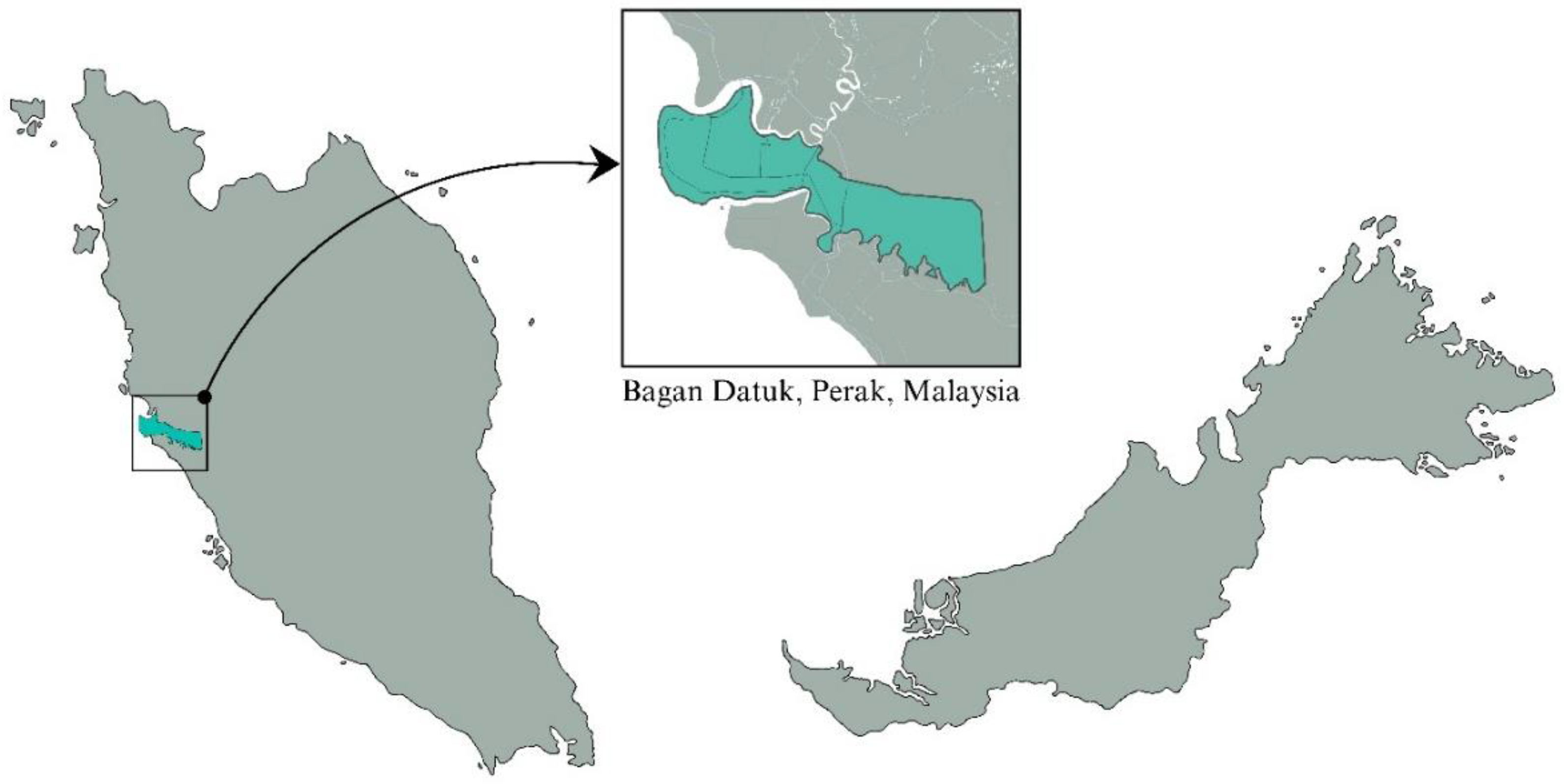
Figure 2.
An overview of zone-wise probe deployment.
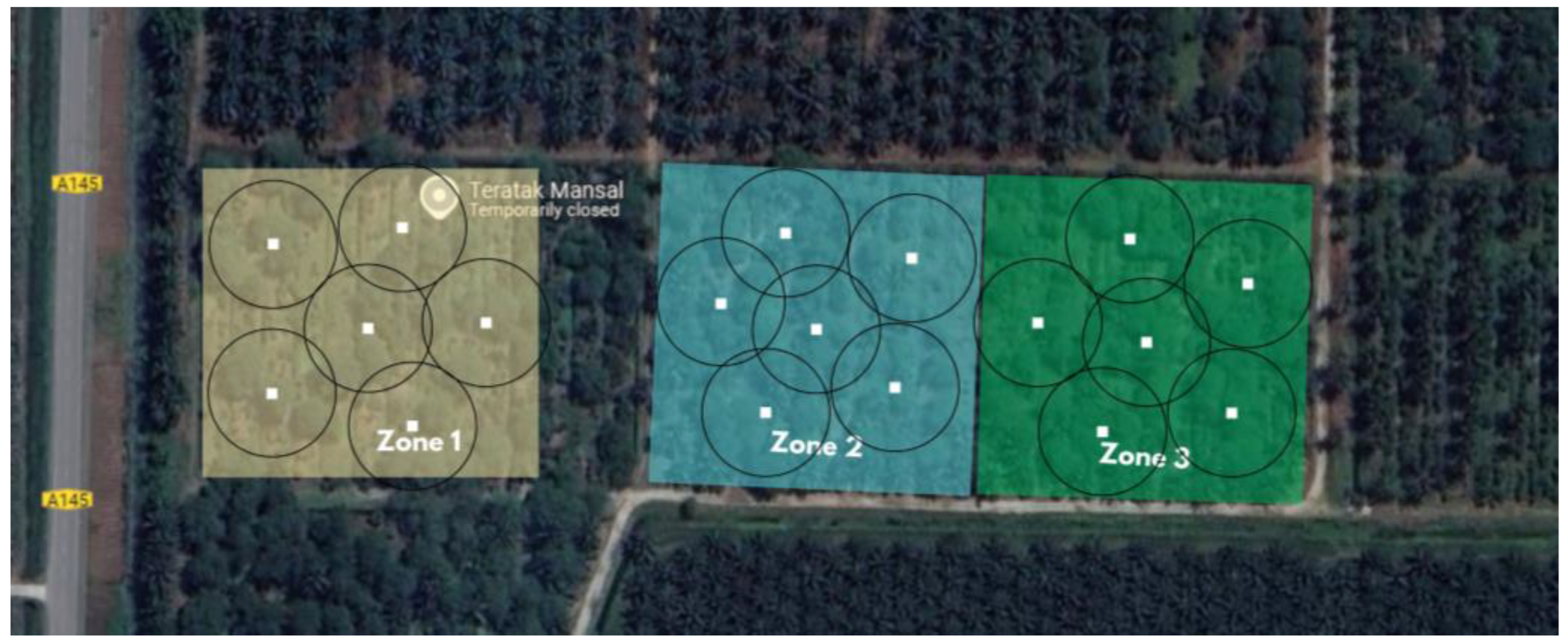
Figure 3.
(a) Illustration of probe within cocoa plant’s rhizosphere; (b) Probe equipped with solar panel and necessary IoT and remote sensing elements; (c) Deployed probe.
Figure 3.
(a) Illustration of probe within cocoa plant’s rhizosphere; (b) Probe equipped with solar panel and necessary IoT and remote sensing elements; (c) Deployed probe.
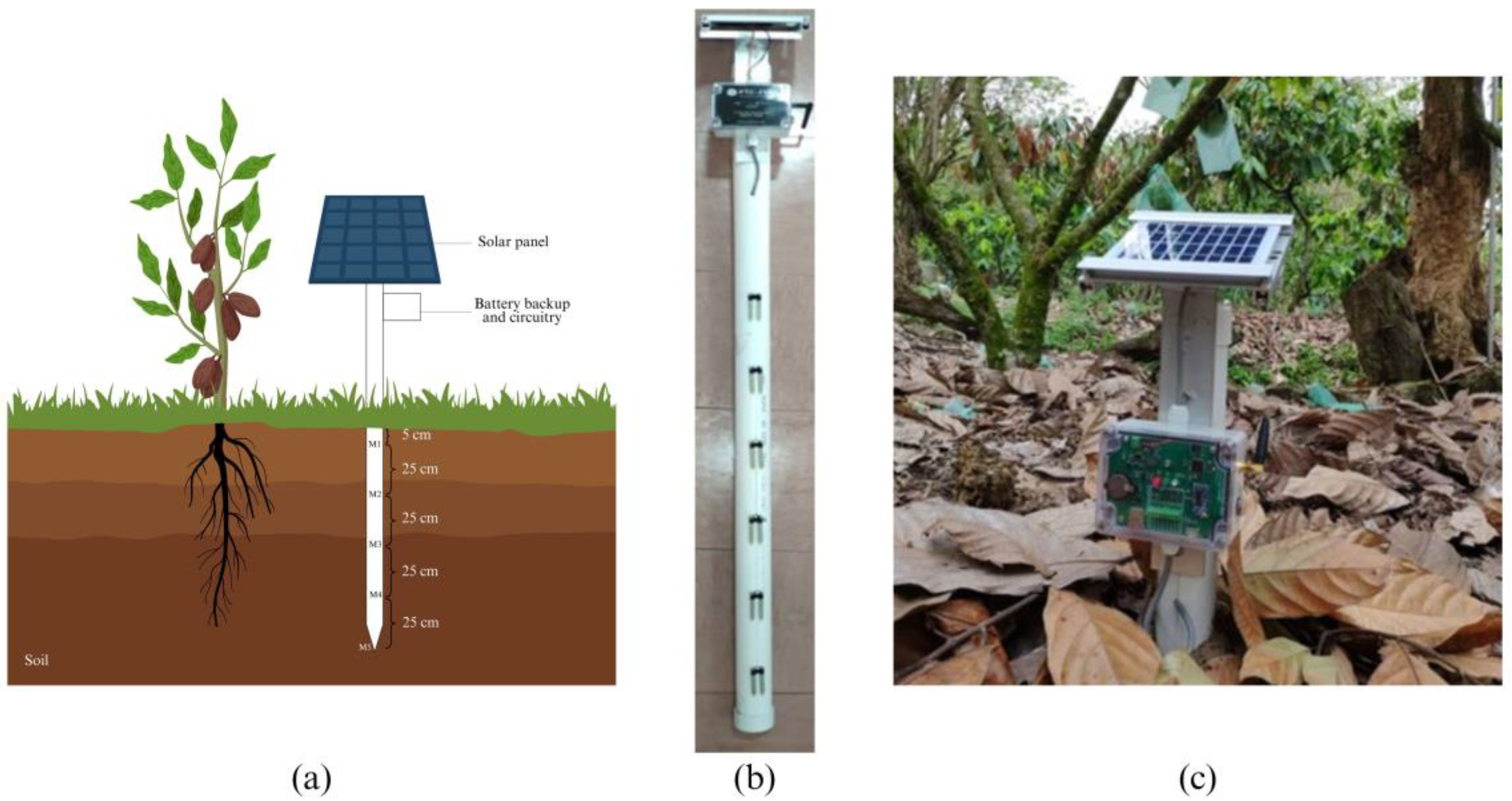
Figure 4.
Architecture of the proposed improved CNN-LSTM model.
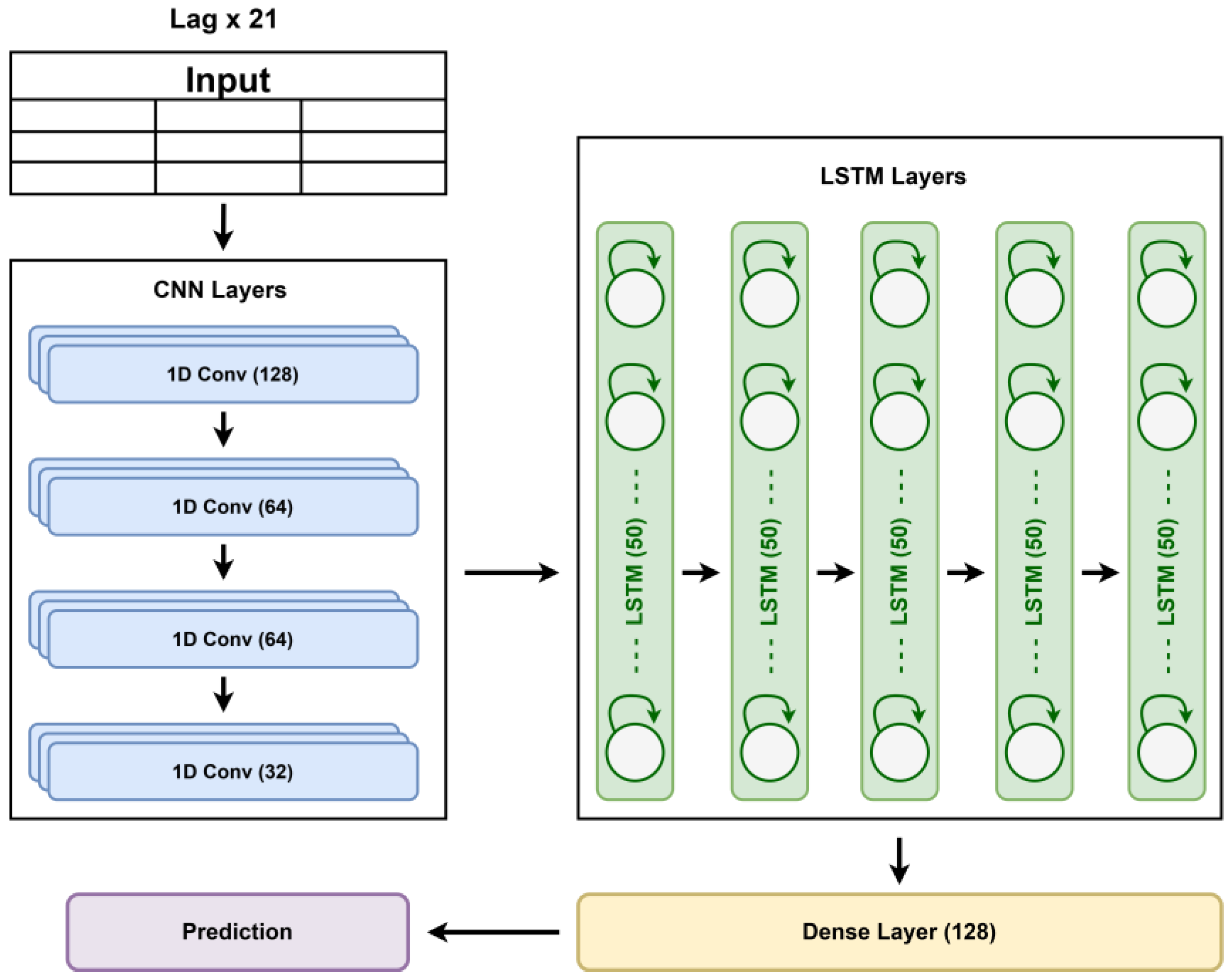
Figure 5.
Correlation matrix of the features for zone 1.
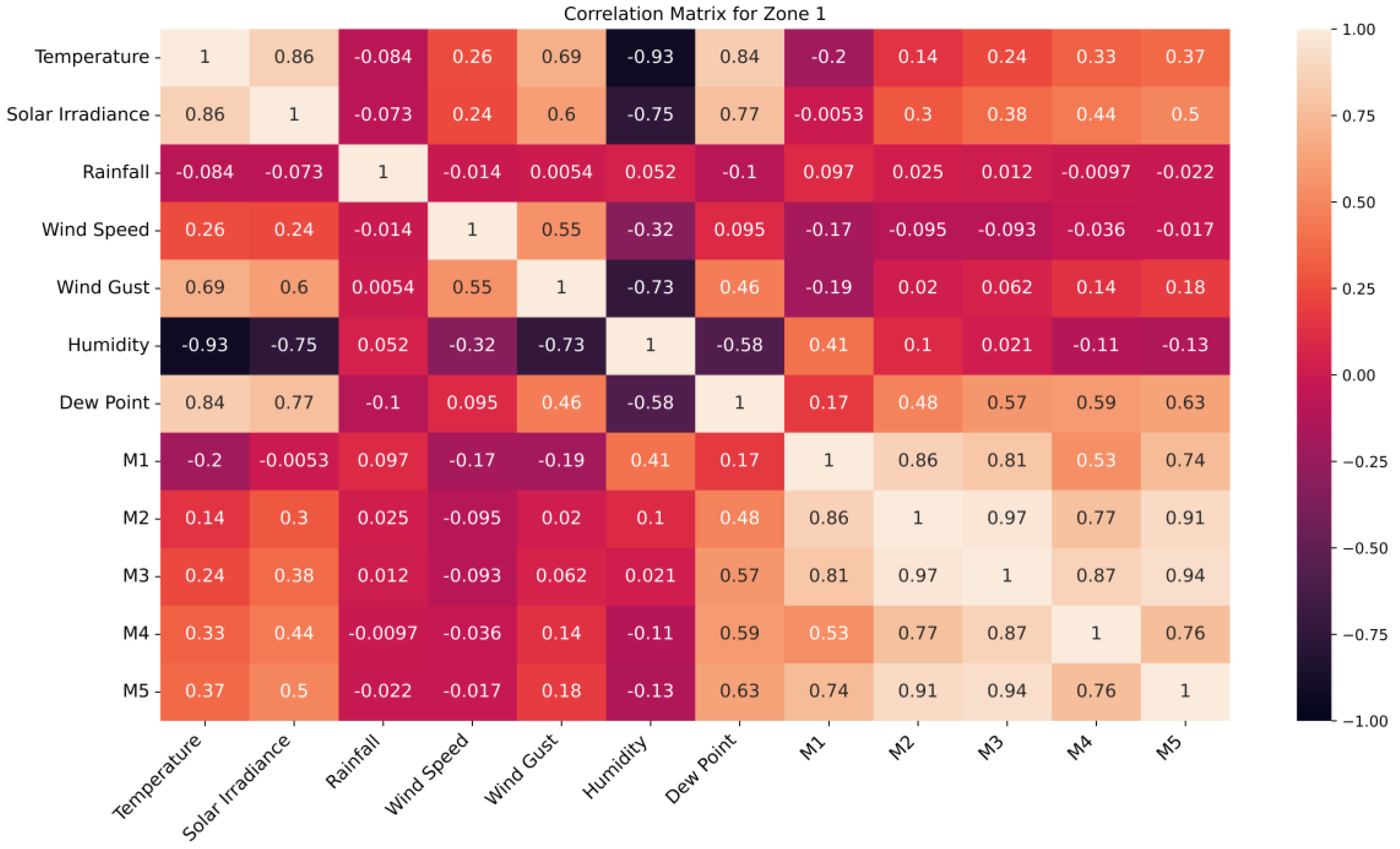
Figure 6.
Correlation matrix of the features for zone 2.
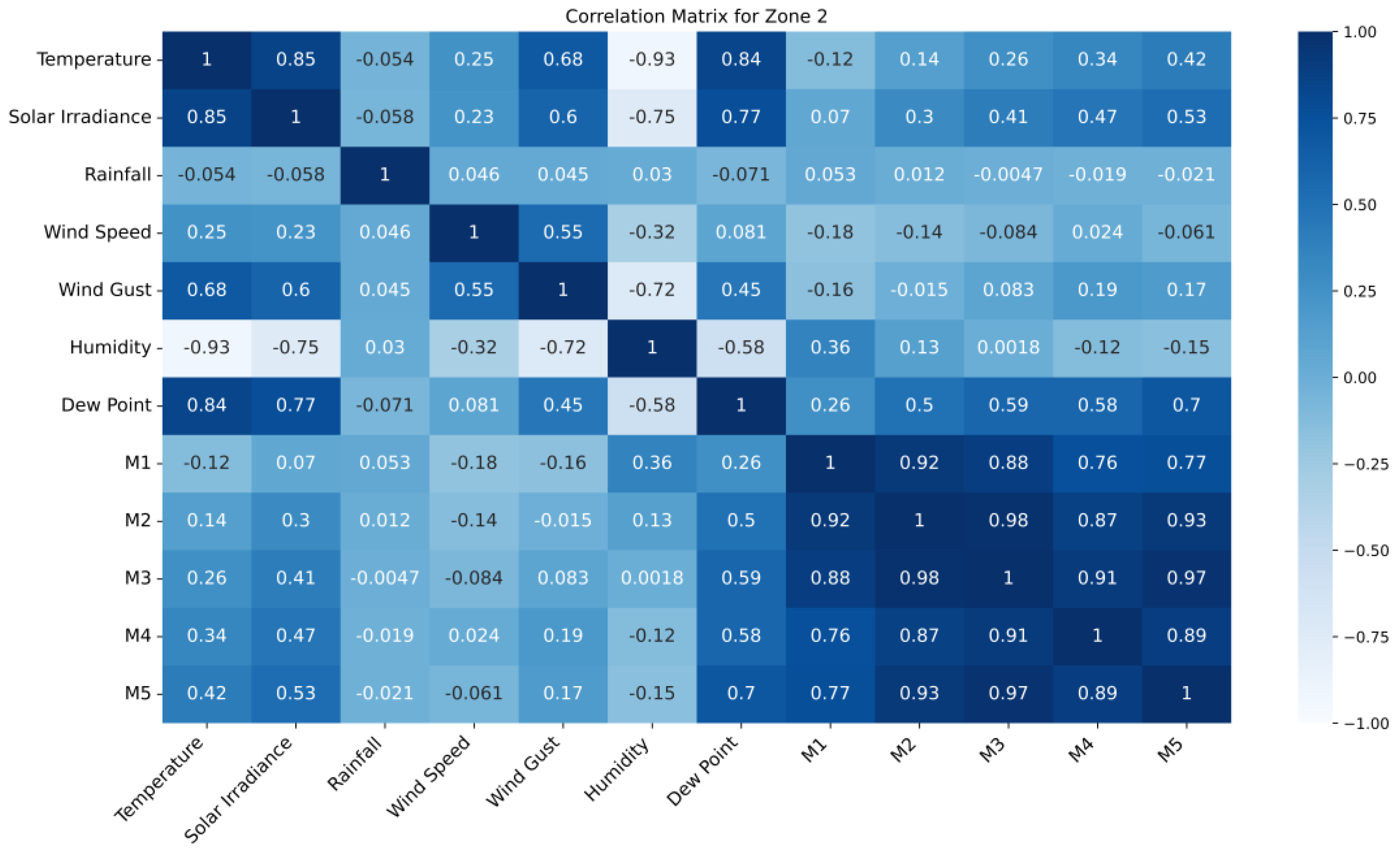
Figure 7.
Correlation matrix of the features for zone 3.
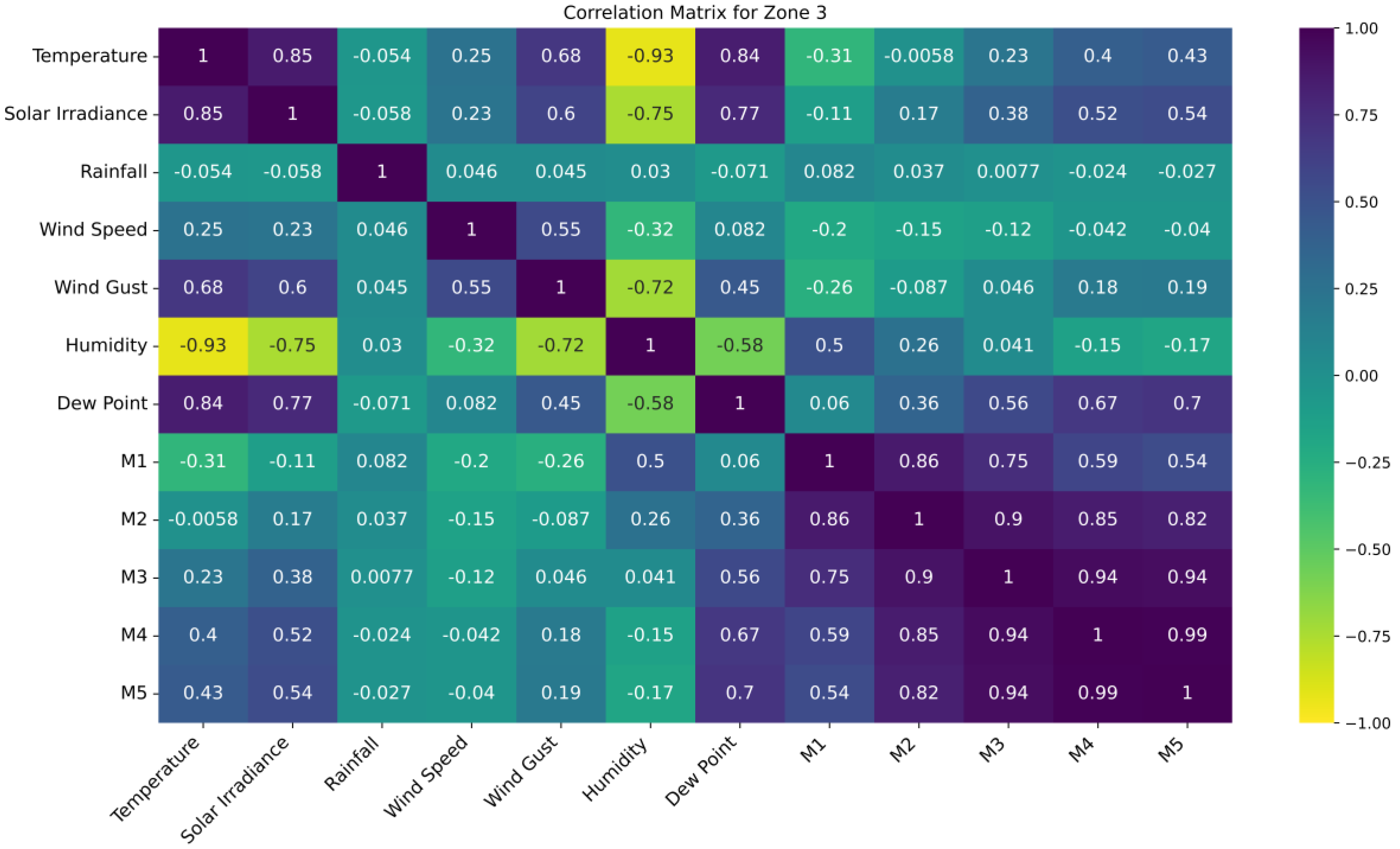
Figure 8.
Heatmap of lag value vs soil layer in terms of R2 in zone 1.
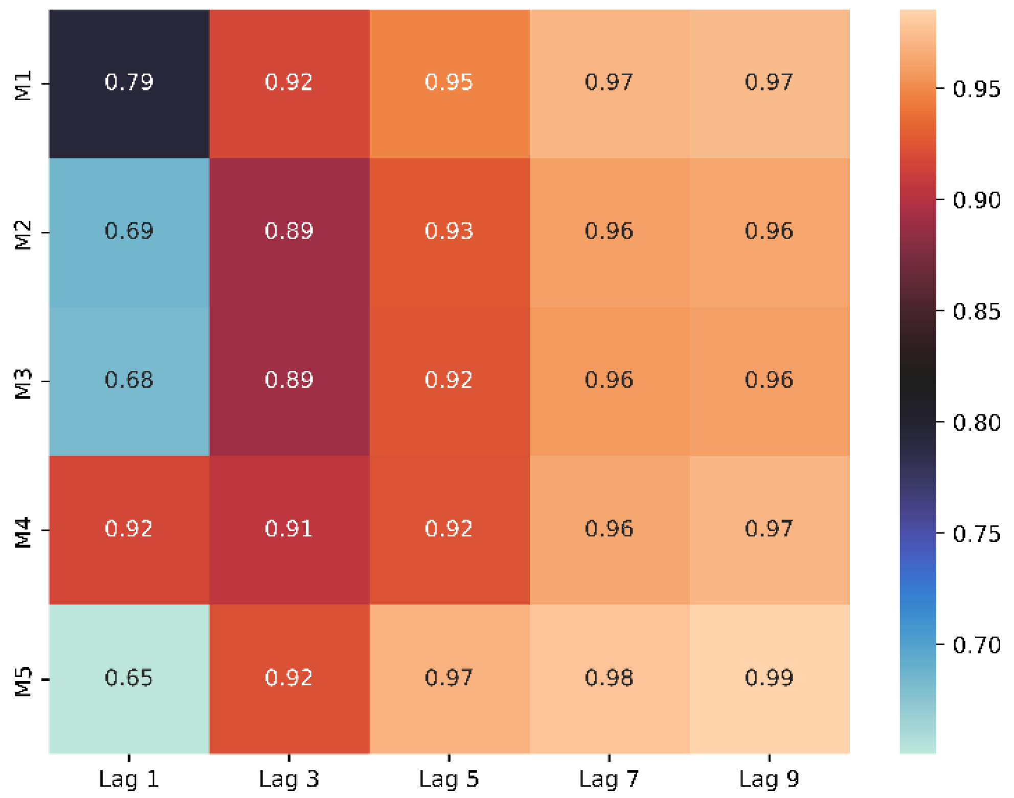
Figure 9.
Actual vs predicted in the 5 layers (M1, M2, M3, M4 and M5) of the soil in zone 1.
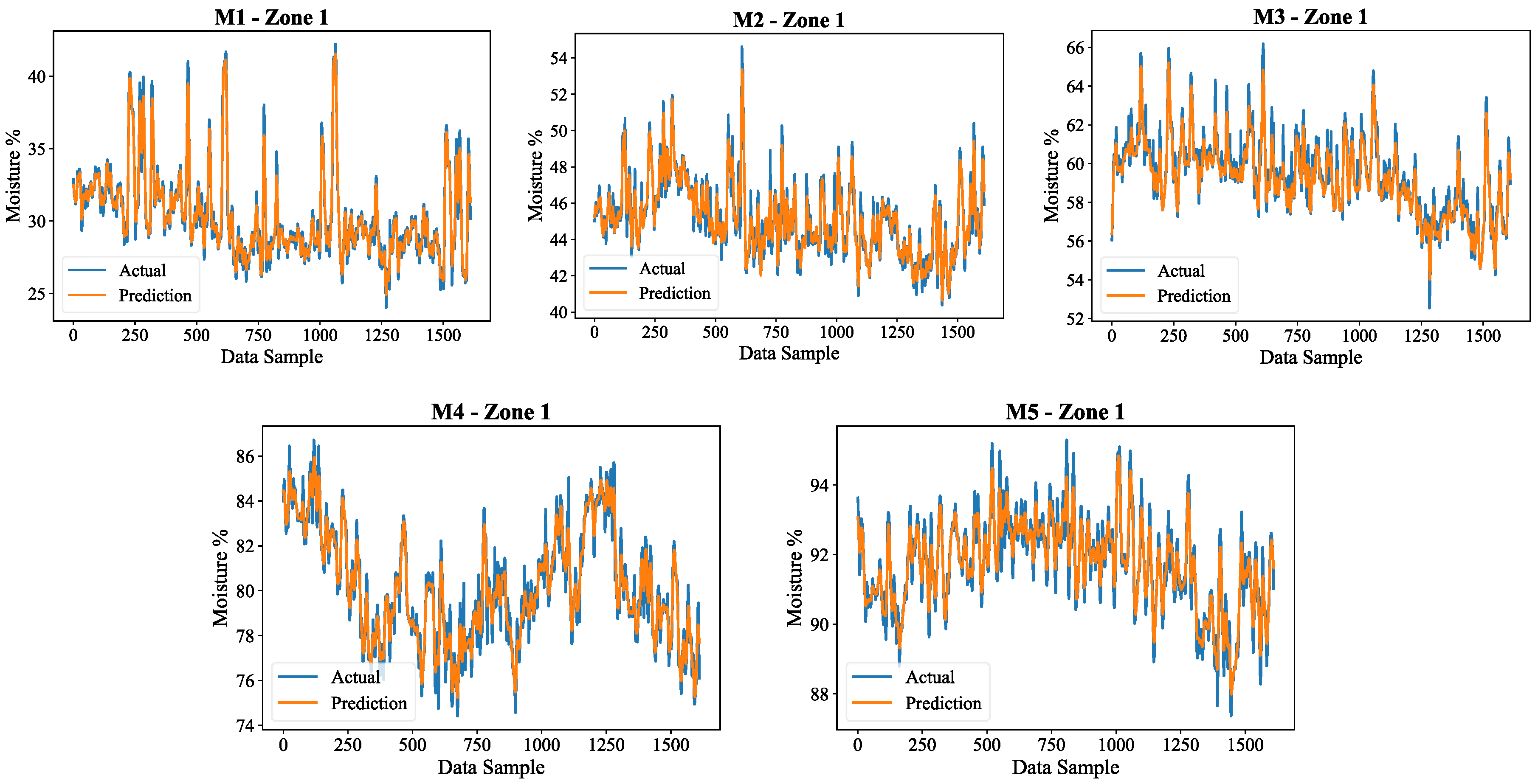
Figure 10.
Scatter plot of the 5 layers (M1, M2, M3, M4 and M5) of the soil in zone 1.
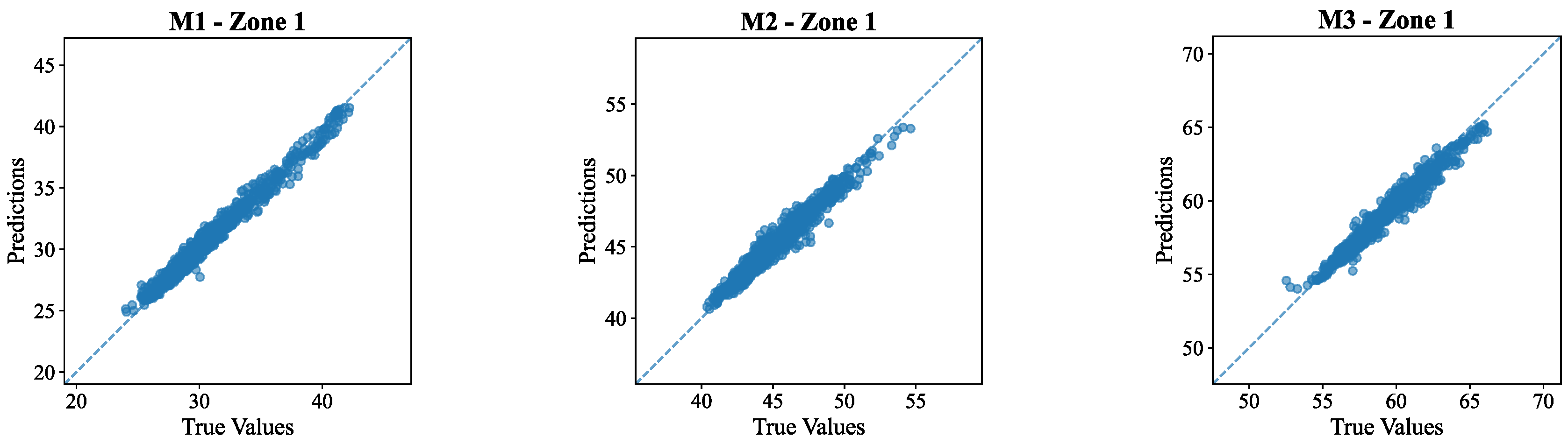
Figure 11.
Heatmap of lag value vs soil layer in terms of R2 in zone 2 and zone 3.
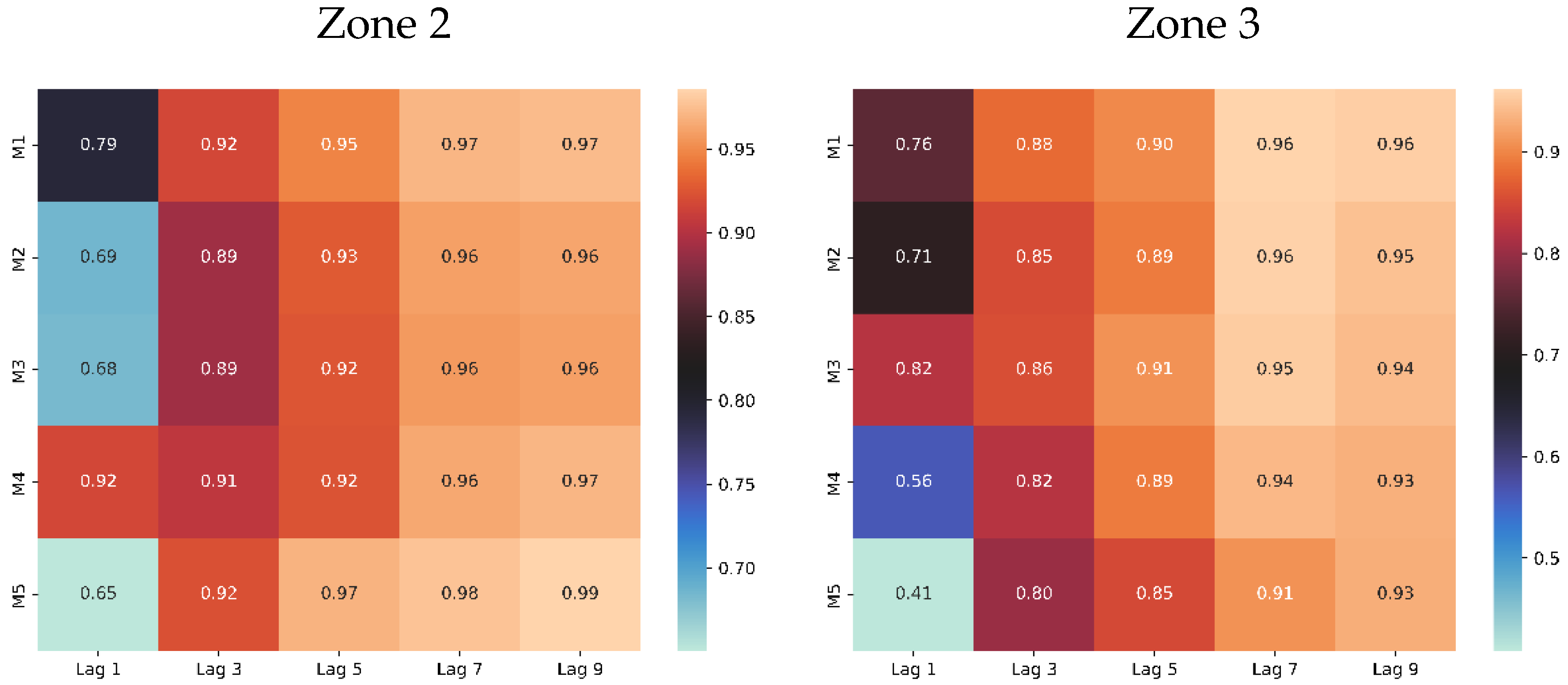
Figure 12.
Actual vs predicted in the 5 layers (M1, M2, M3, M4 and M5) of the soil in zone 2.
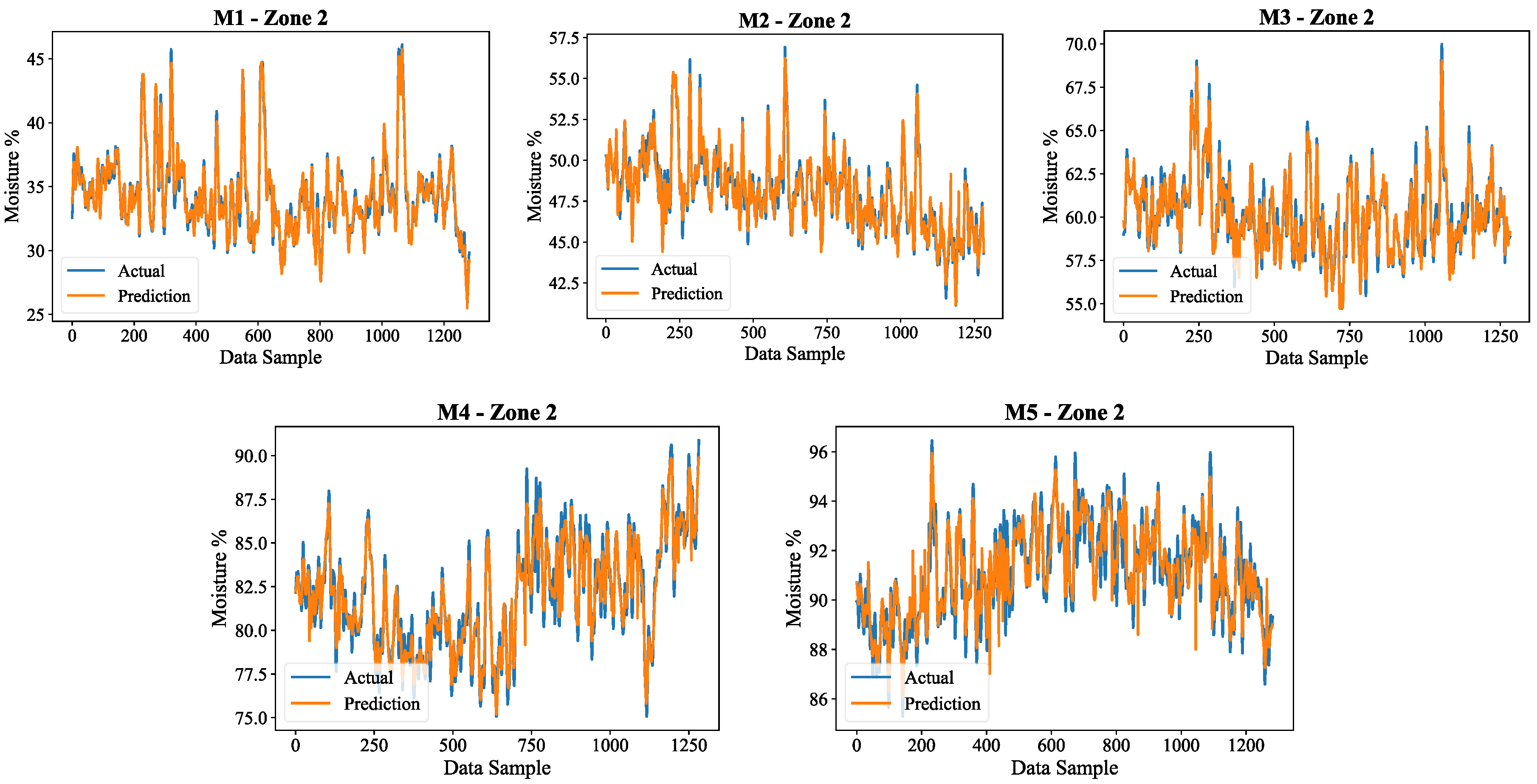
Figure 13.
Actual vs predicted in the 5 layers (M1, M2, M3, M4 and M5) of the soil in zone 3.
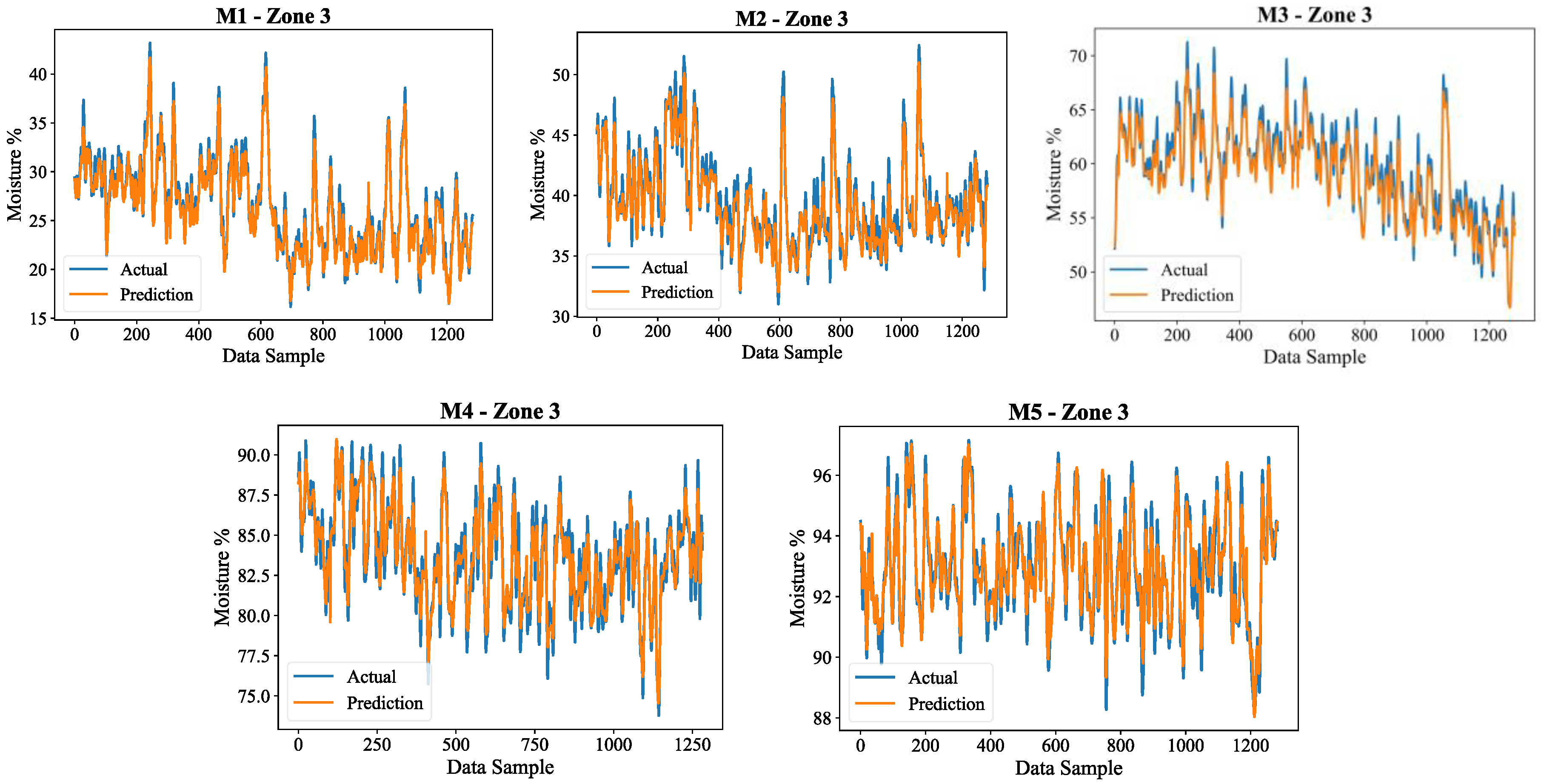
Figure 14.
Scatterplot in the 5 layers (M1, M2, M3, M4 and M5) of the soil in zone 2.
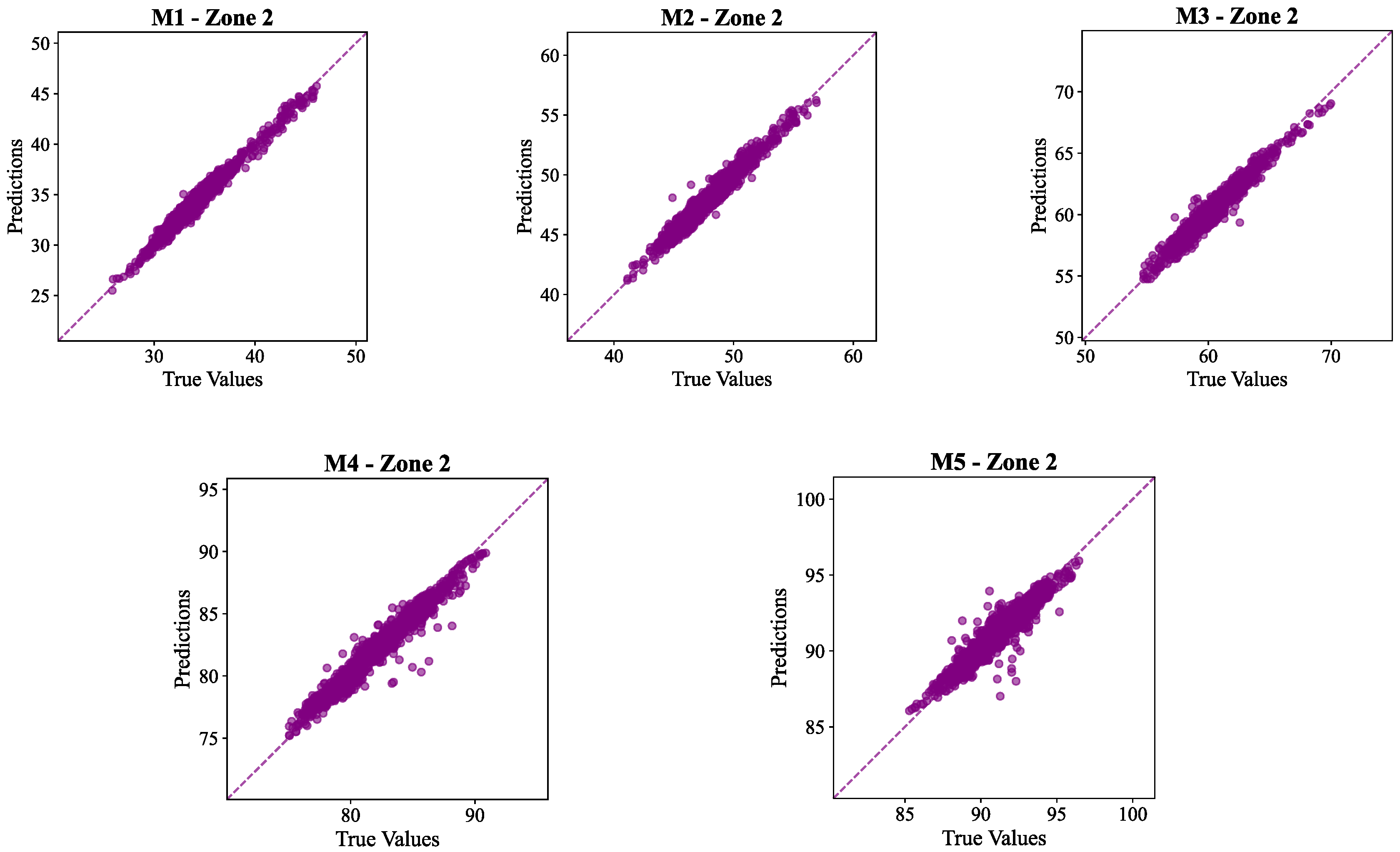
Figure 15.
Scatterplot in the 5 layers (M1, M2, M3, M4 and M5) of the soil in zone 3.
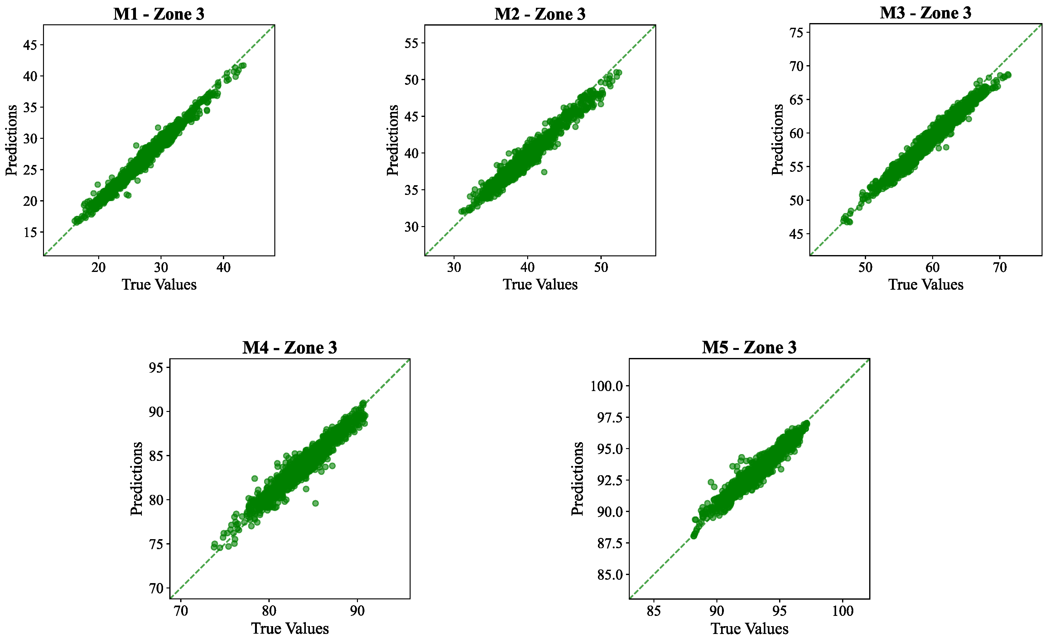
Figure 16.
Feature attributions for soil moisture layer 1 (M1).
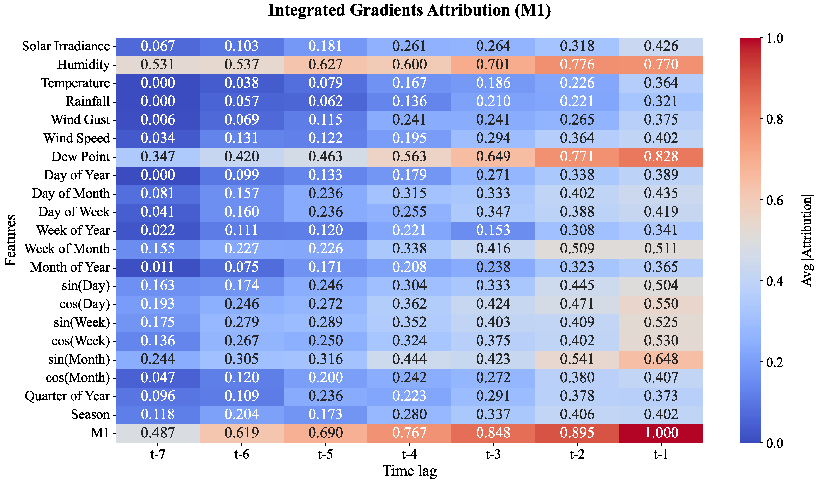
Figure 17.
Feature attributions for soil moisture layer 2 (M2).
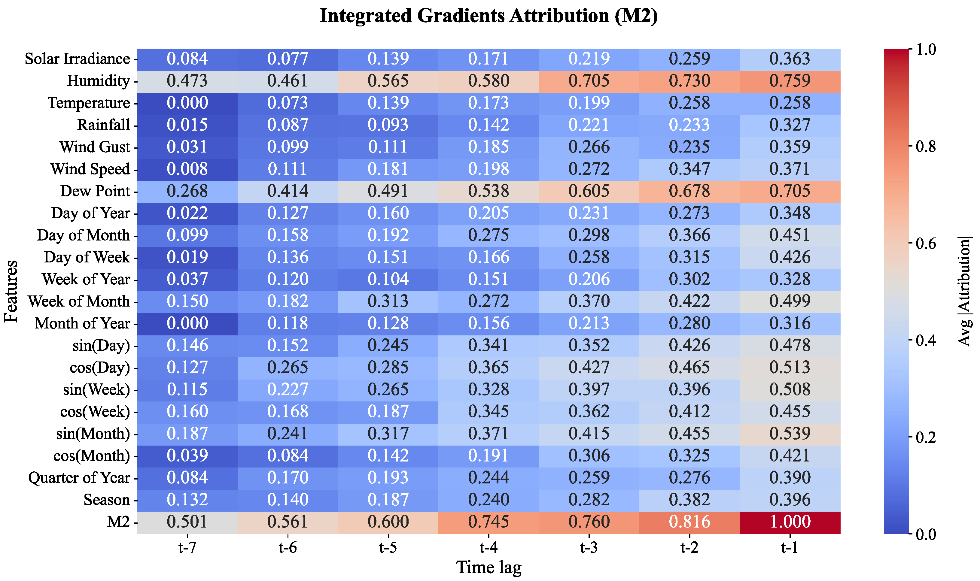
Figure 18.
Feature attributions for soil moisture layer 3 (M3).
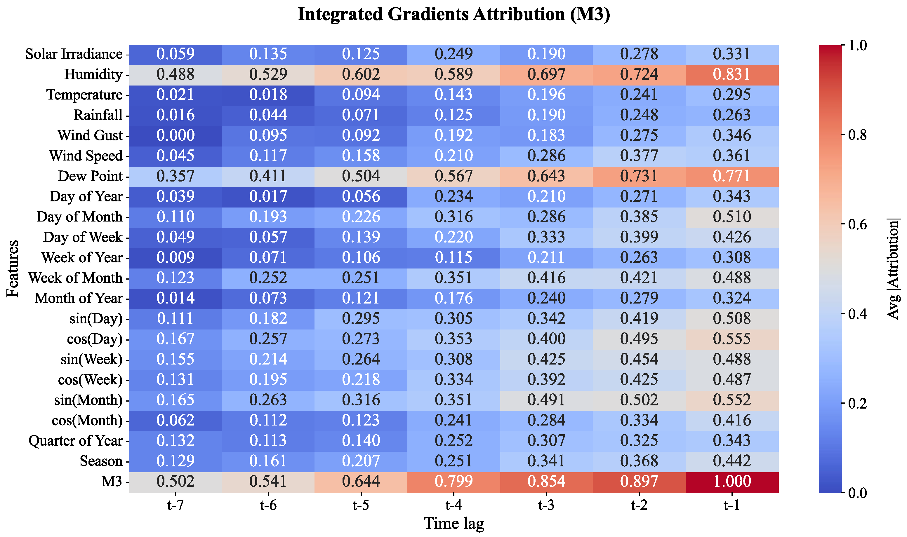
Figure 19.
Feature attributions for soil moisture layer 4 (M4).
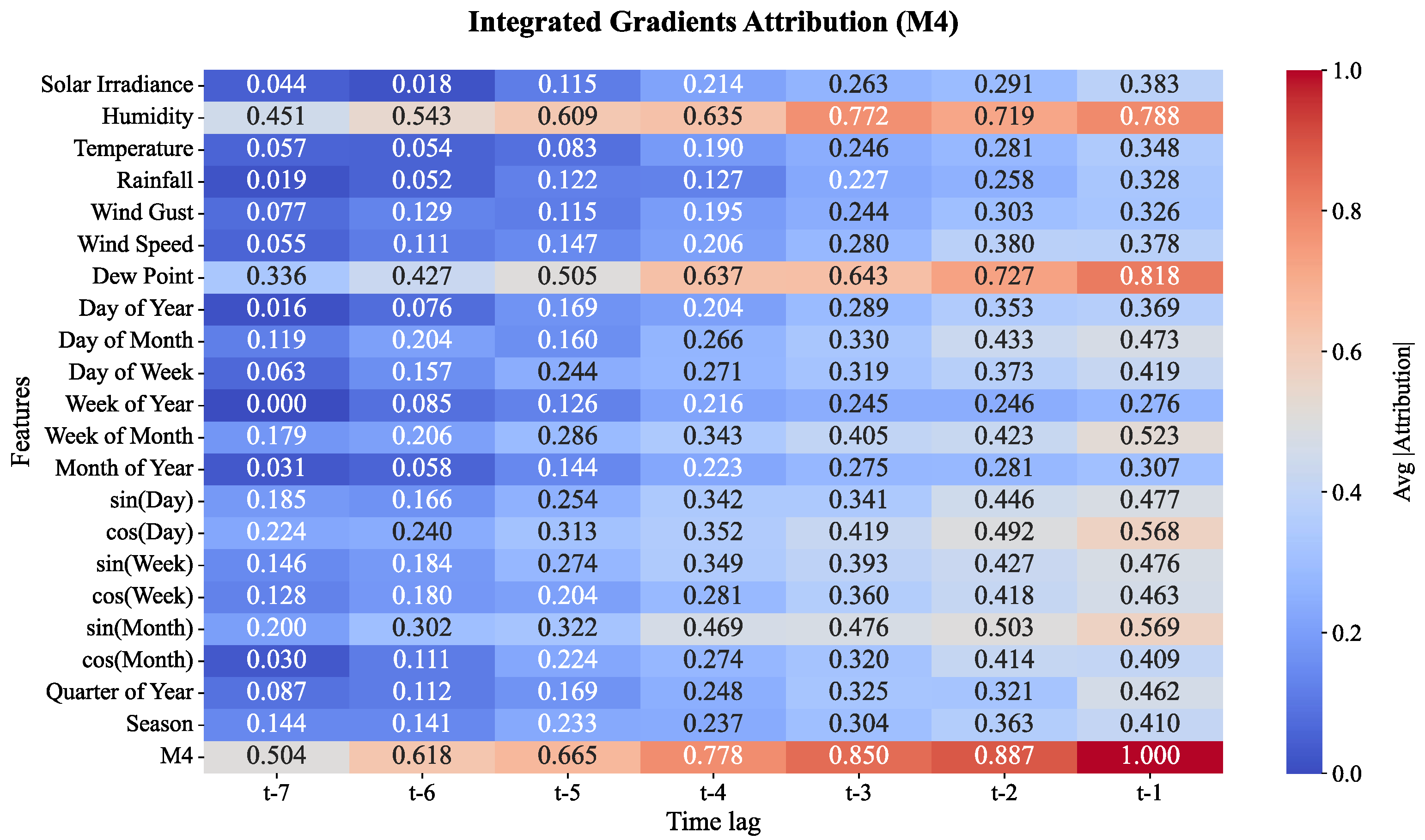
Figure 20.
Feature attributions for soil moisture layer 5 (M5).
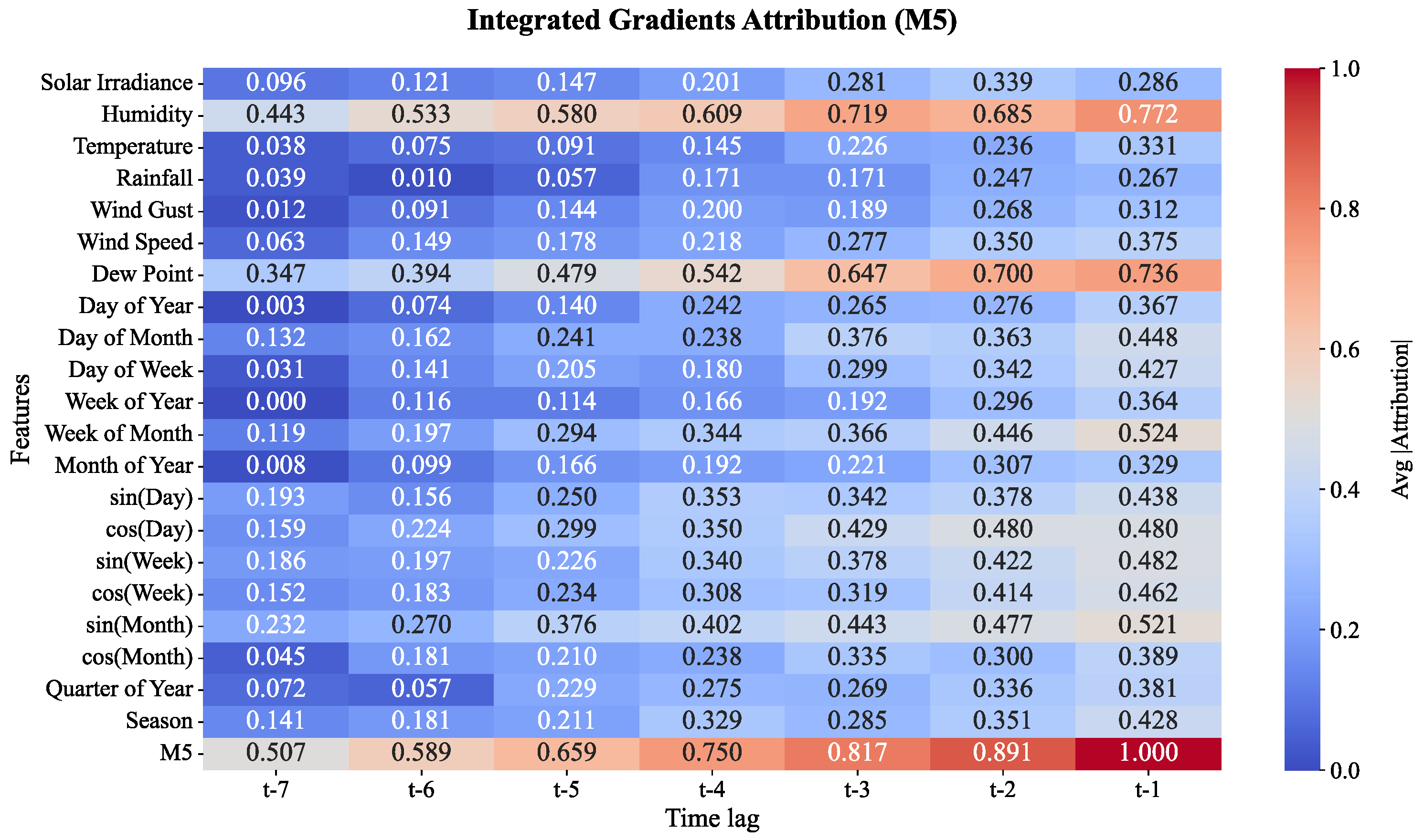
Figure 21.
Prediction plots after adding noise (0%, 5%, 10%, 15% and 20%) for Zone 1 across (a) M1, (b) M2, (c) M3, (d) M4 and (e) M5.
Figure 21.
Prediction plots after adding noise (0%, 5%, 10%, 15% and 20%) for Zone 1 across (a) M1, (b) M2, (c) M3, (d) M4 and (e) M5.
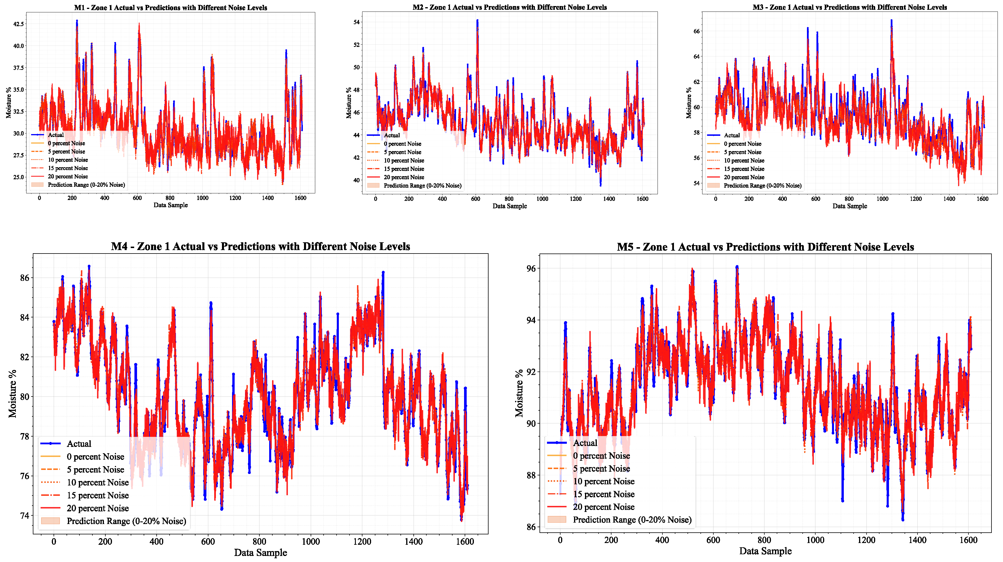

Table 1.
Layers and hyper-parameters of the proposed improved CNN-LSTM architecture.
| Layer Name | Hyper-parameters | Output Shape (Details) |
|---|---|---|
| Input Layer | - | (None, WINDOW_SIZE, 21) - Input shape with 21 features per time step |
| Conv1D (1st) | Filters: 128, Kernel size: 3, Activation Function: Rectified Linear Unit (ReLU) | (None, 64) - Output after 1D convolution, reduced sequence length by 2 due to kernel size |
| Conv1D (2nd) | Filters: 64, Kernel size: 3, Activation Function: Rectified Linear Unit (ReLU) | (None, 64) - Another 1D convolution, sequence length reduces by 2 |
| Conv1D (3rd) | Filters: 32, Kernel size: 3, Activation Function: Rectified Linear Unit (ReLU) | (None, 64) - Another 1D convolution, sequence length reduces by 2 |
| Conv1D (4th) | Filters: 64, Kernel size: 3, Activation Function: Rectified Linear Unit (ReLU) | (None, 64) - Final 1D convolution, sequence length reduces by 2 |
| LSTM (1st) | Units: 50, Recurrent Dropout: 0.1, Return Sequences: True | (None, 50) - Output of LSTM, preserving sequence length for further processing |
| LSTM (2nd) | Units: 50, Recurrent Dropout: 0.1, Return Sequences: True | (None, 50) - Output of LSTM, sequence length preserved |
| LSTM (3rd) | Units: 50, Recurrent Dropout: 0.1, Return Sequences: True | (None, 50) - Output of LSTM, sequence length preserved |
| LSTM (4th) | Units: 50, Recurrent Dropout: 0.1, Return Sequences: True | (None, 50) - Output of LSTM, sequence length preserved |
| LSTM (5th) | Units: 50, Recurrent Dropout: 0.1, Return Sequences: False | (None, 50) - Output of LSTM, final step, no sequence preserved |
| Dense (1st) | Units: 128, Activation Function: Rectified Linear Unit (ReLU) | (None, 128) - Fully connected layer with ReLU activation, output size of 128 |
| Dense (2nd) | Units: 1, Activation: Linear | (None, 1) - Final output layer, output size of 1 (regression output) |
Table 2.
Comparison of training, explanation (IGA), and inference times on CPU and GPU across soil moisture layers (M1–M5) in Zone 1.
Table 2.
Comparison of training, explanation (IGA), and inference times on CPU and GPU across soil moisture layers (M1–M5) in Zone 1.
| Mode | Moisture Level | Train Time | IGA Time | Inference Time |
|---|---|---|---|---|
| CPU | M1 | 10m 15s | 1m 28s | 342ms |
| M2 | 10m 18s | 1m 30s | 341ms | |
| M3 | 10m 20s | 1m 32s | 340ms | |
| M4 | 10m 25s | 1m 35s | 343ms | |
| M5 | 10m 30s | 1m 38s | 345ms | |
| GPU | M1 | 2m 15s | 1m 4s | 130ms |
| M2 | 2m 17s | 1m 6s | 132ms | |
| M3 | 2m 18s | 1m 5s | 131ms | |
| M4 | 2m 22s | 1m 7s | 129ms | |
| M5 | 2m 25s | 1m 9s | 128ms |
Table 3.
Evaluation results for lag 7 of all the layers in zone 1.
| Layer | MSE | RMSE | MAE | MAPE | R² | AVG R² |
|---|---|---|---|---|---|---|
| M1 | 0.5141 | 0.7170 | 0.3024 | 0.0090 | 0.9728 | 0.9704 |
| M2 | 0.4236 | 0.6508 | 0.2694 | 0.0052 | 0.9632 | |
| M3 | 0.4245 | 0.6516 | 0.6516 | 0.0045 | 0.9604 | |
| M4 | 1.0016 | 1.0008 | 1.0008 | 0.0071 | 0.9702 | |
| M5 | 0.5810 | 0.7622 | 0.3145 | 0.0036 | 0.9855 |
Table 4.
Evaluation results for lag 7 of all the layers in zone 2.
| Layer | MSE | RMSE | MAE | MAPE | R² | AVG R² |
|---|---|---|---|---|---|---|
| M1 | 0.2648 | 0.5146 | 0.4035 | 0.0117 | 0.9725 | 0.9435 |
| M2 | 0.3268 | 0.5717 | 0.4428 | 0.0092 | 0.9415 | |
| M3 | 0.2277 | 0.4772 | 0.3797 | 0.0062 | 0.9535 | |
| M4 | 0.4904 | 0.7003 | 0.5108 | 0.0062 | 0.9442 | |
| M5 | 0.3348 | 0.5786 | 0.4201 | 0.0046 | 0.9060 |
Table 5.
Evaluation results for lag 7 of all the layers in zone 3.
| Layer | MSE | RMSE | MAE | MAPE | R² | AVG R² |
|---|---|---|---|---|---|---|
| M1 | 0.7873 | 0.8873 | 0.6947 | 0.0253 | 0.9572 | 0.9411 |
| M2 | 0.8181 | 0.9045 | 0.7072 | 0.0175 | 0.9461 | |
| M3 | 1.0252 | 1.0125 | 0.8202 | 0.0135 | 0.9402 | |
| M4 | 0.7448 | 0.8630 | 0.6509 | 0.0077 | 0.9321 | |
| M5 | 0.2441 | 0.4941 | 0.3653 | 0.0039 | 0.9298 |
Table 6.
Impact of noise injection on model performance at Zone 1 across all the moisture levels.
| Layer | Noise | Zone | MSE | RMSE | MAE | M APE | R² | Layer AVG R² |
|---|---|---|---|---|---|---|---|---|
| M1 | 0% | Zone 1 | 0.2469 | 0.4969 | 0.3748 | 0.0122 | 0.9769 | 0.9343 |
| 5% | Zone 1 | 0.995 | 0.9975 | 0.4782 | 0.0143 | 0.947 | ||
| 10% | Zone 1 | 0.6026 | 0.7763 | 0.6065 | 0.0199 | 0.9218 | ||
| 15% | Zone 1 | 0.71 | 0.8426 | 0.6671 | 0.0219 | 0.9078 | ||
| 20% | Zone 1 | 0.9035 | 0.9505 | 0.7504 | 0.0248 | 0.8827 | ||
| M2 | 0% | Zone 1 | 0.2087 | 0.4568 | 0.353 | 0.0079 | 0.9681 | 0.9297 |
| 5% | Zone 1 | 0.2074 | 0.4555 | 0.35 | 0.0077 | 0.9522 | ||
| 10% | Zone 1 | 0.2504 | 0.5004 | 0.3819 | 0.0085 | 0.9423 | ||
| 15% | Zone 1 | 0.2917 | 0.5401 | 0.4202 | 0.0093 | 0.9327 | ||
| 20% | Zone 1 | 0.3759 | 0.6131 | 0.4793 | 0.0106 | 0.9133 | ||
| M3 | 0% | Zone 1 | 0.1905 | 0.4365 | 0.3424 | 0.0057 | 0.9687 | 0.931 |
| 5% | Zone 1 | 0.2074 | 0.4554 | 0.3426 | 0.0057 | 0.9421 | ||
| 10% | Zone 1 | 0.2389 | 0.4888 | 0.3733 | 0.0063 | 0.9332 | ||
| 15% | Zone 1 | 0.2886 | 0.5372 | 0.4174 | 0.007 | 0.9194 | ||
| 20% | Zone 1 | 0.3579 | 0.5982 | 0.4664 | 0.0078 | 0.9 | ||
| M4 | 0% | Zone 1 | 0.3949 | 0.6284 | 0.484 | 0.0059 | 0.9573 | 0.9299 |
| 5% | Zone 1 | 0.3433 | 0.586 | 0.4578 | 0.0057 | 0.9513 | ||
| 10% | Zone 1 | 0.4226 | 0.6501 | 0.5164 | 0.0064 | 0.9401 | ||
| 15% | Zone 1 | 0.5462 | 0.7391 | 0.5816 | 0.0073 | 0.9226 | ||
| 20% | Zone 1 | 0.6426 | 0.8016 | 0.6365 | 0.0079 | 0.9089 | ||
| M5 | 0% | Zone 1 | 0.1537 | 0.392 | 0.3151 | 0.0034 | 0.9462 | 0.8797 |
| 5% | Zone 1 | 0.2188 | 0.4678 | 0.3757 | 0.0041 | 0.927 | ||
| 10% | Zone 1 | 0.3281 | 0.5728 | 0.4566 | 0.005 | 0.8906 | ||
| 15% | Zone 1 | 0.388 | 0.6229 | 0.497 | 0.0054 | 0.8706 | ||
| 20% | Zone 1 | 0.3963 | 0.6295 | 0.4966 | 0.0054 | 0.8679 |
Table 7.
Evaluation results for lag 7 of all the layers across all three zones.
| Layer | Zone | MSE | RMSE | MAE | MAPE | R2 | AVG R2 | All Zone AVG R2 |
|---|---|---|---|---|---|---|---|---|
| M1 | Zone 1 | 0.5141 | 0.7170 | 0.3024 | 0.0090 | 0.9728 | 0.9675 | 0.9517 |
| Zone 2 | 0.2648 | 0.5146 | 0.4035 | 0.0117 | 0.9725 | |||
| Zone 3 | 0.7873 | 0.8873 | 0.6947 | 0.0253 | 0.9572 | |||
| M2 | Zone 1 | 0.4236 | 0.6508 | 0.2694 | 0.0052 | 0.9632 | 0.9503 | |
| Zone 2 | 0.3268 | 0.5717 | 0.4428 | 0.0092 | 0.9415 | |||
| Zone 3 | 0.8181 | 0.9045 | 0.7072 | 0.0175 | 0.9461 | |||
| M3 | Zone 1 | 0.4245 | 0.6516 | 0.6516 | 0.0045 | 0.9604 | 0.9514 | |
| Zone 2 | 0.2277 | 0.4772 | 0.3797 | 0.0062 | 0.9535 | |||
| Zone 3 | 1.0252 | 1.0125 | 0.8202 | 0.0135 | 0.9402 | |||
| M4 | Zone 1 | 1.0016 | 1.0008 | 1.0008 | 0.0071 | 0.9702 | 0.9488 | |
| Zone 2 | 0.4904 | 0.7003 | 0.5108 | 0.0062 | 0.9442 | |||
| Zone 3 | 0.7448 | 0.8630 | 0.6509 | 0.0077 | 0.9321 | |||
| M5 | Zone 1 | 0.5810 | 0.7622 | 0.3145 | 0.0036 | 0.9855 | 0.9404 | |
| Zone 2 | 0.3348 | 0.5786 | 0.4201 | 0.0046 | 0.9060 | |||
| Zone 3 | 0.2441 | 0.4941 | 0.3653 | 0.0039 | 0.9298 |
Table 8.
Comparative analysis of prediction accuracy of benchmark models.
| Study | Method(s) | Data Sources | Performance Metrics | Key Findings |
|---|---|---|---|---|
| [21] | XGBR with GA optimization | Sentinel-1, Sentinel-2, ALOS DSM | R² = 0.891, RMSE = 0.875% | High-resolution (10 m) SM mapping; suitable for regional-scale water management. |
| [22] | RFR, BRT, SVR | Soil/crop/weather station data | R² = 0.72 (RFR), RMSE = 0.045 m³/m³ | Weather data and rainfall most influential for SM prediction. |
| [29] | NN, RF, SVR | Low-cost soil sensors | R² > 0.92 (1-day NN) | NN with feature selection optimal for short-term SWP forecasts in potatoes. |
| [30] | RF vs. pySEBAL/ EFSOIL | Remote sensing (vineyards) | R² = 0.85 (RF), RMSE = 0.012–0.036 cm³/cm³ | RF outperformed semi-empirical models for RZSM. |
| [31] | RF | Sensor/remote sensing data | R² = 0.84, RMSE = 0.02 cm³/cm³ | RF trained on 70–80% data outperformed semi-empirical models. |
| [28] | Multi-head LSTM ensemble | Aggregated temporal data | R² = 0.95 (monthly) | Weighted ensemble improved long-term SM forecasts. |
| [25] | Conv-LSTM + XAI | Meteorological/static variables (China) | R² = 0.92, MAE = 0.028 m³/m³ | Precipitation most critical; SG revealed regional SM dynamics. |
| [23] | CNN-LSTM, Bi-LSTM | Climate/soil data | R² = 0.9838, RMSE = 0.3672 | CNN-LSTM leveraged spatio-temporal features best. |
| [24] | LSTM | Sentinel-1, SMAP, climate | R² = 0.87, RMSE = 0.046 | Best performance in arid/low-vegetation regions. |
| [26] | CLA (CNN-LSTM-Attention) | Hydrus-1D simulations, MODIS | R² = 0.9298 (80–100 cm) | Physical + DL integration reduced RMSE by 49–57%. |
| [32] | LSTM vs. Triple Collocation | SMAP/AMSR2/ASCAT fusion | ubRMSE = 0.052 cm³/cm³, R = 0.77 | LSTM captured spatio-temporal variability better. |
| [33] | CNN-LSTM | UAV (RGB, multispectral, thermal) | R² = 0.80–0.88, RMSE = 2.46–2.99 m³/m³ | Multi-sensor fusion boosted accuracy in citrus. |
| [20] | Hybrid LSTM + Aquacrop 7.0 | Soil/weather/satellite (maize) | R² = 0.8163–0.9181 | Aquacrop-simulated data enhanced LSTM predictions. |
| Proposed Study | Hybrid LSTM+CNN | Soil and weather | R² = 0.9517, RMSE = 0.71908 | Development of an improved hybrid CNN-LSTM model for accurate multi-layer soil moisture prediction in root zone for Cocoa plantations. |
Disclaimer/Publisher’s Note: The statements, opinions and data contained in all publications are solely those of the individual author(s) and contributor(s) and not of MDPI and/or the editor(s). MDPI and/or the editor(s) disclaim responsibility for any injury to people or property resulting from any ideas, methods, instructions or products referred to in the content. |
© 2025 by the authors. Licensee MDPI, Basel, Switzerland. This article is an open access article distributed under the terms and conditions of the Creative Commons Attribution (CC BY) license (http://creativecommons.org/licenses/by/4.0/).
Copyright: This open access article is published under a Creative Commons CC BY 4.0 license, which permit the free download, distribution, and reuse, provided that the author and preprint are cited in any reuse.


