Submitted:
03 March 2025
Posted:
04 March 2025
You are already at the latest version
Abstract
Distinguishing galaxies as either fast or slow rotators plays a vital role in understanding the processes behind galaxy formation and evolution. Standard techniques, which are based on the λR-spin parameter obtained from stellar kinematics, frequently face difficulties to classify fast and slow rotators accurately. These challenges arise particularly in cases where galaxies have complex interaction histories or exhibit significant morphological diversity. In this paper, we evaluate the performance of a Convolutional Neural Network (CNN) on classifying galaxy rotation kinematics based on stellar kinematic maps from the SAMI survey. Our results show that the optimal CNN architecture achieves an accuracy and precision of approximately 91% and 95% on the test dataset, respectively. Subsequently, we apply our trained model to classify previously unknown rotator galaxies for which traditional statistical tools have been unable to determine whether they exhibit fast or slow rotation, such as certain irregular galaxies or those in dense clusters. We also used Integrated Gradients (IG) to reveal the crucial kinematic features that influenced the CNN’s classifications. This research highlights the power of CNNs to improve our comprehension of galaxy dynamics and emphasizes their potential to contribute to upcoming large-scale Integral Field Spectrograph (IFS) surveys.
Keywords:
galaxy
; kinematics
; classifications
; CNN
1. Introduction
One of the key factors in investigating galaxy formation and evolution is defining the spin of the galaxy (rotation). As outlined by [1], the spin parameter () provides a robust way to quantify the stellar angular momentum in galaxies. This parameter enables a clear distinction between fast and slow rotators, representing different evolutionary paths and formation mechanisms [2,3,4]. Fast rotators, characterized by high values, are thought to have formed through gas-rich minor mergers or secular processes, including the inflow of external gas [5]. In contrast, slow rotators, characterized by low values, are believed to result from dissipationless processes, such as dry minor mergers [6,7]. Furthermore, they note that the distribution of values in different environments can provide insights into the role of galaxy interactions and environmental effects on galaxy evolution [8,9,10,11,12,13].
The methods for measuring galaxy spin have evolved significantly over the years, encompassing both observational and theoretical approaches. A significant advancement came with the introduction of the parameter [14], which compared the ratio of rotation velocity to velocity dispersion and was introduced as an indicator of the observed rotation [15]. In this method, integrated quantities such as and are measured, representing the sky-averaged values of V (velocity) and (velocity dispersion)1, as observed using integral-field spectrographs like SAURON [1]. However, this method has limitations. For instance, galaxies such as NGC 3379, which exhibits global rotation, and NGC 5813, which shows spatially confined non-zero velocities, yield similar values despite having distinct kinematic structures. On the other hand, the advent of integral-field spectroscopy, allowing for spatially resolved kinematics across entire galaxies. This led to the development of the parameter by [1], which provided a more robust measure of specific angular momentum.
The origin of angular momentum captured by the kinematic parameter , has been a topic of significant theoretical interest. For instance, [16] propose an explanation for the origin of angular momentum in dark matter halos. On the theoretical front, numerical simulations have played a crucial role in understanding the origins and evolution of galaxy spin. In particular, [17] conducted hydrodynamical simulations to show that the topology of the merging regions (specifically the number of intersecting filaments), accurately predicts the spin of both dark matter and gas. They found that halos located at the centres of knots exhibit low spin, whereas those at the centres of filaments exhibit high spin.
Upcoming sky surveys, such as the Hector instrument [18,19] and the Wide-field Spectroscopic Telescope (WST) [20], are expected to provide even larger databases with billions of galaxies. However, identifying slow/fast rotators within such an enormous number of galaxies cannot be achieved using traditional statistical methods and requires specialized tools. Convolutional neural networks (CNNs) [21], a branch of machine learning models, have gained prominence in cosmology and astronomy. Their power lies in elucidating patterns within complex datasets, proving to be highly effective for diverse scientific tasks. In the field of exoplanet detection, CNN methods have been employed to enhance the process of identification and examination of potential exoplanets from large-scale datasets [22,23]. In radio astronomy, deep learning approaches like DECORAS [24] has been applied to differentiate and characterize radio-astronomical sources. They have also been helpful in Active galactic nuclei (AGNs) data [25] such as detection and classification of AGN host galaxies [26]. They have also been valuable in strong lensing searches [27,28,29], improving efficiency by reducing the time required while enhancing accuracy. Furthermore, CNNs have proven to be valuable in cosmology, showing potential to address computational limitations faced by conventional statistical methods in dark energy [30,31,32], dark matter [33,34,35], Cosmic Microwave Background (CMB) maps [36,37,38], and Gravitational Wave (GW) [25,39,40]. These applications showcase the remarkable versatility and capability of CNNs n deepening our understanding of the universe. [41,42,43] provided an extensive overview of CNN applications in addressing a wide range of astronomical and cosmological challenges.
In this study, we leverage CNNs to classify galaxies as slow or fast rotators based on their stellar kinematics maps. We adopt a supervised learning approach, utilizing labeled data from the SAMI catalog as our training, testing, and validation datasets2. Through this process, we seek to find the best CNN architecture, achieving an accuracy of approximately 91% on the test dataset. Subsequently, we apply our trained model to classify previously unknown rotators galaxies for which traditional statistical tools have been unable to determine whether they exhibit fast or slow rotation. We utilized interpretability techniques, including Integrated Gradients (IG), to uncover the key kinematic features that guided the CNN’s classification decisions. Ultimately, this work highlights the effectiveness of CNNs in distinguishing between slow and fast rotators, demonstrating their potential to advance our understanding of galaxy dynamics and informing future observational strategies.
The structure of this paper is organized as follows. In Section 2, we describe the data source, preprocessing steps, and dataset preparation from the SAMI survey [44,45], which are used for the CNN-based classification of slow and fast galaxy rotators. In this section, we also provide a detailed explanation of the network architecture, data preprocessing, and evaluation methods. Our results and their physical interpretations are discussed in Section 3. In this Section, we also present a series of studies aimed at elucidating how our CNN model makes decisions when classifying images. Finally, we discuss and summarize the main results of this work in Section 4.
2. Dataset and Machine Learning Methods
The data source used in this study is the SAMI survey. The SAMI instrument [44] was installed on the 3.9 meter Anglo-Australian Telescope (AAT) and connected to the AAOmega spectrograph [46,47,48,49,50,51]. This setup provides a median resolution of in the range of and in the range of [52]. We concentrate on a sample that includes stellar kinematics, selecting only the Brightest Group Galaxies (BGGs) with stellar masses of , ensuring the inclusion of massive galaxies with high signal-to-Noise (S/N > 5). In our study, we processed a dataset comprising 2,444 galaxies containing stellar kinematics data from the SAMI survey. We systematically iterated through the directory containing the galaxies FITS (Flexible Image Transport System) files, and extracting relevant information from each file. Specifically, we retrieved the primary data array from each FITS file and associated it with a unique identifier derived from the its filename. Then, we stored these data arrays and their corresponding identifiers in separate files.
For our data processing pipeline, we applied several crucial steps to ensure data quality and relevance for our analysis of galaxy stellar kinematics. First, we addressed the issue of duplicated labels in our dataset and removed any duplicate entries from our label array, ensuring each galaxy in our sample was represented uniquely. Thereafter, we handled missing values in our stellar kinematics data by replacing NaN values with zeros, a common practice in astronomical data processing when dealing with regions of low signal-to-noise ratio. We categorised galaxies based on their rotational properties. Based on the spin-ellipticity relations from [53], we categorized each galaxy as either a fast rotator (designated as 1) or a slow rotator (designated as 0). Finally, to standardize our spatial analysis, we extracted a central region of each galaxy’s kinematic map, creating a consistent spatial scale across our sample. By selecting a square region of pixels centered on each galaxy, we ensured that our analysis focused on the most relevant and well-measured parts of each galaxy while maintaining a uniform spatial coverage across our sample. These data processing steps were crucial in preparing a clean, consistent, and well-characterized dataset for making our training, test and validation datasets. These datasets can used in our CNN binary classification problem. Then, we applied a CNN to classify stellar kinematics maps that were previously labeled as fast or slow rotators.
2.1. Convolutional Neural Network Architecture
CNNs is a highly effective and widely used technique for object recognition and classification in the field of Machine Learning (ML) [54]. These neural networks employ a hierarchical architecture consisting of multiple layers, including convolutional and pooling operations. Through this architecture, the CNN can automatically learn and extract meaningful features from input images, enabling it to process complex visual data with remarkable accuracy [55]. In our study, we applied a CNN on two-dimensional stellar kinematics maps to distinguish fast/slow rotators.
We employed a systematic approach to design an optimal CNN architecture for classifying galaxies based on their stellar kinematic properties. We utilized Keras Tuner [56], an automated hyperparameter optimization framework, to explore a wide range of model configurations efficiently. We varied the number of convolutional layers (between 1 and 4), the number of filters in each layer (from 32 to 256 in steps of 32), and the learning rate (choosing from 1e-2, 1e-3, or 1e-4). This approach enabled us to systematically evaluate different model complexities and training parameters. The resulting optimal architecture, as determined by Keras Tuner is showed in Table 1.
In the CNN architecture, our goal is to minimise the binary cross-entropy loss. To achieve this, we employ the Adam optimiser [57] with a learning rate of 0.0002 and a beta parameter () of 0.9. Additionally, we implemented two checkpoints in the model. The first one is the ModelCheckpoint, which saves the best model during training based on the validation accuracy. The second one is the ReduceLROnPlateau, which reduces the learning rate when there is no progress in training. Moreover, we incorporate the EarlyStopping callback, which stops the training process if the validation accuracy does not improve. To monitor the training progress, we recorded the loss function and accuracy computed on the training data after each epoch. We also calculate the validation loss and accuracy on a separate validation dataset. These metrics provide insights into the performance of the model during training and helped track its progress.
2.2. Data Preprocessing
We enhanced our dataset using a custom data augmentation function. This function takes the original data and labels as input and applies various transformations to generate additional training samples, thereby increasing the diversity of the training set. Specifically, we utilized the ImageDataGenerator from Keras, configured with parameters such as a rotation range of 360 degrees, width and height shifts of up to 4 pixels, zoom range from 1.0 to 1.05, and horizontal flipping, with the fill mode set to nearest to maintain the integrity of the images. To balance the number of fast and slow rotator samples in the dataset, the function performed seven times more augmentations on the slow rotator samples. These transformed images were added to the dataset along with their corresponding labels, ensuring an equal representation of fast and slow rotators.
After preprocessing, the dataset consists of 1,112 samples, with 980 classified as fast rotators and 132 as slow rotators. To address the class imbalance, we applied data augmentation, specifically aimed at balancing the number of slow and fast rotators. As a result, the final dataset comprises 19,332 samples, with 9,603 fast rotators and 9,729 slow rotators, ensuring a more balanced distribution for training the model. Then we divided it into three subsets: 70% for training, 15% for testing, and the remaining for validation. This split ensured that the model was trained on a substantial portion of the data, while also being evaluated and validated on separate, unseen subsets to gauge its performance and generalization capabilities. This augmentation and splitting strategy was crucial for improving the robustness and accuracy of our CNN in classifying stellar kinematics maps as fast or slow rotators.
2.3. Loss Function
Loss functions are used to evaluate our network’s accuracy by measuring the inequality between predicted and true class labels. For our binary classification problem of distinguishing fast from slow rotators, we employed the Binary Cross Entropy (BCE) [58] loss function. Optimization was carried out using the Adam optimizer with a learning rate of 0.001 and the BCE loss function is formulated as:
In this context, corresponds to the actual class label of the ith sample within our dataset of N training samples, and is the probability predicted by the model for the ith sample being a fast or slow rotator.
2.4. Evaluation Criteria
To evaluate and compare the effectiveness of the CNN on the test dataset, it is crucial to establish appropriate evaluation criteria. In the context of stellar kinematics maps, which is treated as a classification problem distinguishing between fast/slow rotators samples, we can utilize the following confusion matrix for evaluation purposes:
In this context, True Positive (TP) indicates correctly identified fast rotator, True Negative (TN) corresponds to accurately recognized slow rotator, False Positive (FP) denotes misclassification of slow rotator sources as fast one, and False Negative (FN) refers to fast rotator missed by the algorithm and classified as slow one.
| True Data | |||
| Test Results | Fast | Slow | |
| Fast | TP | FP | |
| Slow | FN | TN | |
These terms allow us to define various evaluation metrics. Accuracy measures the fraction of correctly identified samples (TP and TN) out of the total number of samples. Precision quantifies the ratio of true positives to the sum of true positives and false positives, showing the reliability of positive predictions [59]. These metrics are defined as:
The Receiver Operating Characteristic (ROC) curve [60] is another useful metric, which depicts the trade-off between TP and the FP for the CNN model. Each point on the ROC curve corresponds to a different threshold for categorizing samples as slow or fast rotator based on their predicted probabilities. By analyzing the ROC curve, we can determine how well the model distinguishes between fast and slow rotator samples. A model with superior performance will have a curve that closely approaches the top-left corner of the plot, signifying a higher TP rate and a lower FP rate for various thresholds.
3. Results
In this section, we present the results that show the performance of our CNN-based model in classifying fast and slow rotator using the stellar kinematics maps from the SAMI survey. We first investigate the model’s classification performance through the confusion matrix and the ROC curve, and analyse the distribution of the model’s predictions. Afterward, we apply the CNN model to unknown rotational samples and analyze the key features in the stellar maps that influence its decision-making process. To achieve this, we utilize an explainable CNN approach, including Integraded Gradients (IG).
3.1. Training CNN on Galaxies with Known Fast/Slow Rotation
Using SAMI observations, the stellar kinematics maps of galaxies can be estimated and the parameter is used as a proxy for the spin parameter. Following [1] it is calculated using:
where the subscript i refers to the ith spaxel within the ellipse, is the flux of the ith spaxel, is the stellar velocity in km s−1, and is the velocity dispersion in km s−1. We train the CNN on a training data including stellar kinematics maps with the defined 7697 fast and 7835 slow rotators which defined by the parameter .
In Figure 1 we show the confusion matrix for the CNN model which is demonstrates a strong performance of the model, especially in terms of precision, suggesting that it effectively minimizes false positives for the slow rotator category. The overall accuracy further reinforces the model’s reliability in making predictions between the two classes. Since the model output represents the probability of an object being a fast rotator, ranging between 0 and 1, setting a threshold is necessary to classify objects into two classes: fast and slow rotators. Figure 2 illustrates the ROC plot which is followed a steep ascent, quickly reaching high TP rates even at low FP rates, which is indicative of a strong classifier. The Area Under the ROC Curve (AUC) is reported as 0.95, which is very close to the ideal value of 1.0. This high AUC score suggests that the model has excellent discriminative ability between the slow/fast rotator category. Figure 3 reveals a distribution for both the CNN predictions (blue) and the real data (pink). There are two prominent peaks at the extreme ends (0 and 1) for both distributions, indicating that the model is making confident predictions for a large number of samples, classifying them as either strongly slow rotators (close to 0) or strongly fast rotators (close to 1). The CNN’s predictions closely align with the real data distribution, especially at the extremes. This suggests that the model is performing well in identifying clear-cut cases. However, there are some discrepancies in the middle range (around 0.2 to 0.8), where the CNN shows more varied predictions compared to the real data. This could indicate that the model is less certain about borderline cases and produces a wider range of probability estimates for these samples.
Figure 4 displays different visualizations of false positive samples from the CNN model. Each visualization represents a different instance where the model incorrectly classified a slow rotator sample as a fast one. Figure 5 displays visualizations of false negative samples from the CNN model. Each visualization represents a different instance where the model incorrectly classified a fast rotator sample as a slow one. These false positive and false negative cases are crucial for understanding where and why the model is making mistakes. They could represent edge cases or challenging inputs that share some characteristics with positive samples, leading to misclassification. Analyzing these false positives can provide insights into the model’s decision-making process and highlight areas where it might be overfitting or misinterpreting certain features. This information is valuable for refining the model, adjusting its architecture, or enhancing the training data to improve overall performance and reduce such misclassifications in future iterations.
3.2. Testing the CNN on Unknown Rotators
Figure 7 illustrates the CNN prediction probabilities for unknown fast and slow rotator samples. Traditional techniques that rely on the -spin parameter derived from stellar kinematics often face significant challenges, including the misclassification of galaxies with complex rotation patterns and the inability to effectively analyze low surface brightness galaxies [61]. These limitations stem from the conventional methods’ struggles to capture the intricate details of stellar motion across diverse galaxy environments. For example, galaxies with non-axisymmetric features or those affected by interactions with neighboring galaxies can yield misleading values. Moreover, low surface brightness galaxies, which often exhibit considerable structural complexity, may fall below the detection thresholds of standard techniques, resulting in gaps in our understanding of their dynamics.
Figure 6.
Histogram of CNN prediction probabilities (P) for unknown samples. The distribution is marked by two threshold regions: fast rotators (, red dashed line) and slow samples (, blue dashed line). The total count of fast () and slow () samples are 678 and 39 respectively.
Figure 6.
Histogram of CNN prediction probabilities (P) for unknown samples. The distribution is marked by two threshold regions: fast rotators (, red dashed line) and slow samples (, blue dashed line). The total count of fast () and slow () samples are 678 and 39 respectively.
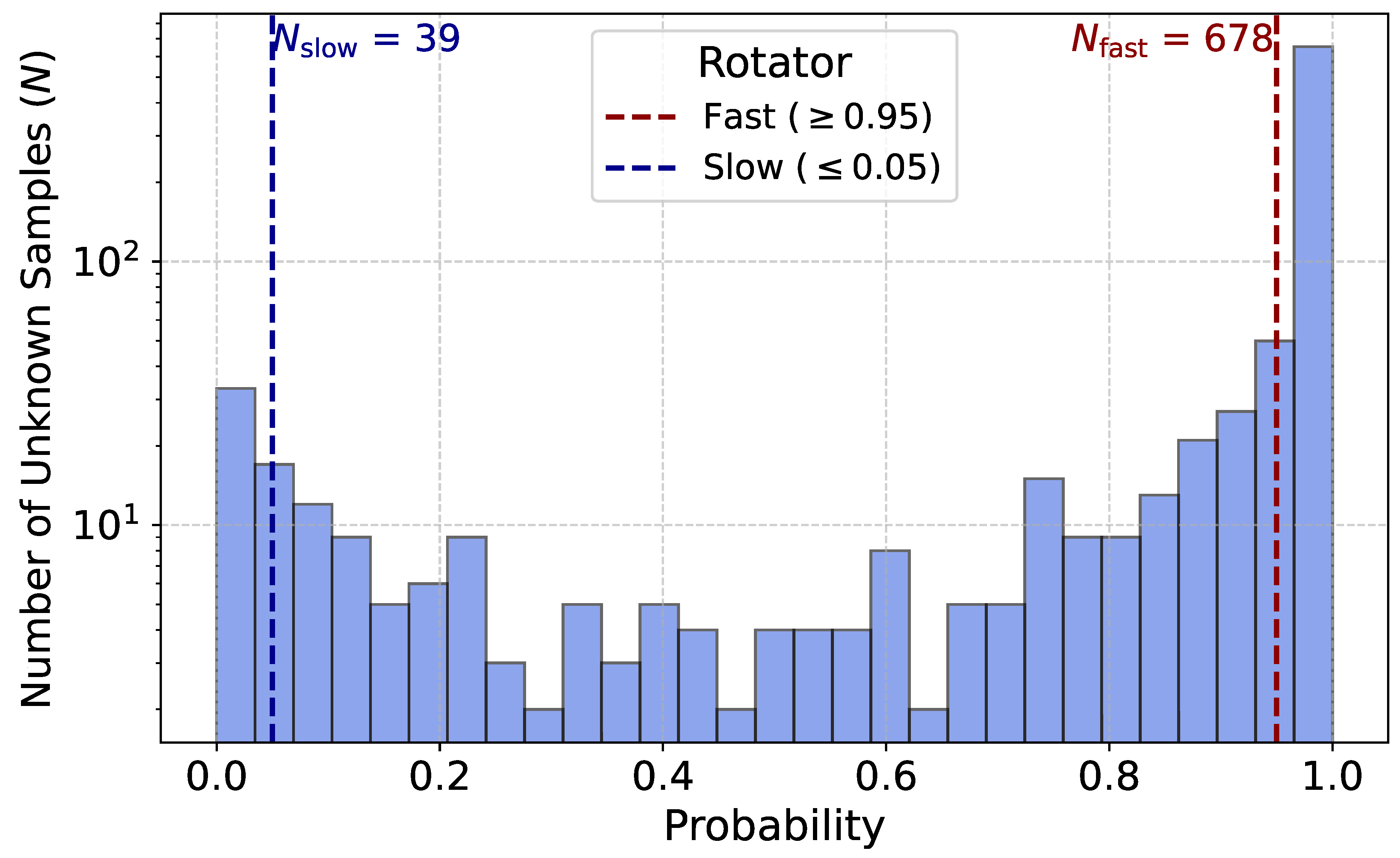
Among the 1,112 samples in the SAMI catalogue, a significant portion, 854 samples were not classified as either slow or fast rotators due to these limitations. To tackle these complexities, we utilize the strengths of CNNs, which are adept at recognizing patterns in high-dimensional data. By training our CNN on stellar kinematic maps, we can effectively identify subtle variations in rotational dynamics that traditional methods might miss. In Figure 7, we present the probability distribution of our CNN model’s predictions for the unknown samples. In this analysis, we consider samples with a probability greater than 0.95 as fast rotators and those with a probability lower than 0.05 as slow rotators. Based on this criterion, our model identifies 678 fast rotators and 39 slow rotators.
The CNN’s capability to learn from extensive datasets enables it to discern and classify intricate rotational signatures, thereby enhancing the accuracy of galaxy classification. This methodology not only improves our ability to categorize fast and slow rotators but also allows us to investigate previously ambiguous cases involving complex rotations or low surface brightness galaxies, ultimately advancing our comprehension of galaxy formation and evolution.
3.3. Interpretability of the Model’s Classifications
This subsection outlines a series of studies aimed at elucidating how our CNN model arrives at its decisions when classifying images. Two primary techniques are used to gain insight into the decision-making processes of the CNN model:
(i) Measuring the clustering of velocity variations in the stellar kinematics maps using Global Moran’s I (GMI) tool [62,63].
(ii) Utilizing Integrated Gradients (IG) [64] to emphasize the areas of input images that significantly respond to the fast or slow classes.
We analyze the histograms of GMI values for the fast and slow rotators, emphasizing the significance of clustering in high- and low-velocity stars for defining these categories. Afterwards, we employ IG to identify key regions within the velocity stellar maps that influence the decision-making process of our CNN model. Finally, we investigate the model’s decisions for true positives and true negatives cases, exploring the relationship between clustering in velocities of stars and the IG values outcomes.
3.3.1. Clustering of High- and Low- Velocity Stars
Visual inspection of the velocity variations in the stellar kinematics maps reveals a more pronounced clustering of high- and low-velocity stars in fast rotators compared to slow rotators. In this direction, we utilize the GMI tool to assess the spatial autocorrelation of stellar maps by considering both the locations and values of features simultaneously. Specifically, these observed patterns indicate a clustering of high- and low-velocity stars within the stellar maps. GMI index value measure the spatial autocorrelation, which quantifies how similar or dissimilar data values are based on their spatial proximity. It’s often used in spatial statistics to determine whether there is clustering, dispersion, or randomness in a data sample. The formula for the GMI index is:
where n is the number of observations, is the value of the variable of interest at location i, is the mean of the variable, is the spatial weight between locations i and j. The interpretation of the GMI index value can be categorized as follows:
(i): Positive GMI index (close to +1): Indicates clustering or positive spatial autocorrelation, meaning similar values (either high or low) tend to be close to each other.
(ii): Negative GMI index (close to -1): Indicates dispersion or negative spatial autocorrelation, suggesting that high and low values are intermixed and tend to avoid clustering.
(iii): Zero or near-zero GMI index: Suggests a random spatial pattern with no clear clustering or dispersion.
Figure 8 shows the histograms of GMI values for fast and slow rotators. The distribution shows that there are significantly more slow rotators in the lower ranges (0.0 to 0.4) of Moran’s I. The fast rotators more prominently in the middle to higher ranges (approximately 0.4 to 1.0), suggesting a different distribution pattern between the two categories. In Figure 9 we show the spatial autocorrelation in star velocities maps for two fast rotators from the SAMI dataset which is predicted correctly by our CNN model. The central scatter plot presents Moran scatter plot for each fast rotator, where the spatial lag of standardized velocity is plotted against the standardized star velocity. High Moran’s I values (0.910, and 0.930) indicate strong spatial autocorrelation in all cases, suggesting coherent kinematic structures within these fast rotators. The top row shows spatial velocity maps, with red and blue regions indicating higher and lower velocities, respectively. In contrast, in Figure 10 we show the previous analysis for the two slow rotators. Lower Moran’s I values (0.385, and 0.180) suggest weaker spatial autocorrelation, indicating less coherent kinematic structures compared to the fast rotating galaxies.
The examination of stellar kinematics and the Global Moran’s I (GMI) index reveals substantial differences between fast and slow rotators in terms of velocity distribution. Fast rotators exhibit more distinct clustering of both high and low velocities, with GMI values between 0.4 and 1.0, indicating a higher degree of spatial autocorrelation and more uniform kinematic structures. Conversely, slow rotators display lower GMI values (0.0 to 0.4), pointing to weaker spatial autocorrelation and less coherent velocity distributions. This suggests that fast rotators have more cohesive velocity arrangements than slow rotators, which exhibit more scattered and irregular distributions.
3.3.2. Integrated Gradients
Integrated Gradient (IG) [64] is a systematic method used to evaluate the contribution of individual pixels or regions in an input image to the model’s final classification decision. To thoroughly understand IG, it is crucial to explore the concept of alpha, a key parameter in this approach. Alpha, is a real number ranging from 0 to 1. It establishes a path along which the gradients of the model’s predicted probabilities are evaluated. Specifically, dictates the proportional contribution of information from a baseline image relative to the target image being analysed. This proportional contribution is calculated as an integral along the defined path. Recently IGs has numerous applications in astronomy, including strong lensing searches [65] and weak lensing analysis [66].
IG is applied on the slow and fast rotators in the Figure 9 and Figure 10, respectively. In Figure 9, in the right row of each sample, we show the IG value for each pixels of these samples. It should be noted that pixels with IG values higher than zero have positive effect on the our model decision and vice versa. The majority of these IG images highlight the pixels in the coherent kinematic structures in the image. So according to this analysis we can say one of the the CNN model features that is used in distinguishing fast and slow rotators is the coherent kinematic structures in the fast rotators. While, in Figure 10, slow rotators IG images the majority of pixels are concentration in the weaker spatial autocorrelation, indicating less coherent kinematic structures.
4. Discussion and Conclusions
In this work, we have demonstrated the success of convolutional neural networks (CNNs) in effectively classifying galaxies into fast and slow rotators based on their stellar kinematic maps. Using data from the SAMI survey, we developed and fine-tuned a CNN architecture that delivered an accuracy of 91% and a precision of 95%, proving its reliability in distinguishing between the two categories. These results illustrate the the potential of the CNNs to overcome challenges in galaxy classification, particularly when traditional methods relying on -spin parameters, encounter uncertainties.
The analysis of stellar kinematics using the Global Moran’s I (GMI) index reveals distinct differences between fast and slow rotators in their velocity distributions. This suggests that fast rotators have more organized and structured velocity fields, whereas slow rotators exhibit more scattered and irregular distributions, highlighting fundamental differences in the kinematic properties of slow and fast rotators. The interpretability of CNN classifications is a important component of this study. By applying Integrated Gradients, we uncovered the primary kinematic feature that that significantly effected the model’s outputs. Our findings indicate that the CNN focuses on coherent kinematic structures within stellar velocity maps to classify galaxies, confirming its ability to detect meaningful physical patterns. Using this interpretable CNN model we can enhance confidence in the model’s predictions.
The scalability and adaptability of CNNs are essential given the emergence of current and future large-scale integral field spectroscopy (IFS) surveys, such as the Hector instrument [18,19] which is designed to characterize 15,000 galaxies and Wide-field Spectroscopic Telescope (WST) [20], which generate datasets comprising billions of galaxies. Under this condition, traditional statistical approaches will face significant challenges in handling such extensive data effectively. Our findings highlight the vital role of CNNs for processing and analysing stellar kinematic patterns in these large datasets, establishing their importance for the next generation of astronomical exploration.
Although the findings are promising, the study highlights some limitations. The model showed uncertainty in borderline cases, as shown in the probability distribution of predictions. Addressing this will need for larger and more diverse training datasets. Future research could aim to include expanding the approach to account for advanced kinematic features, like higher-order velocity moments, or leveraging transfer learning with pre-trained models on similar datasets. Furthermore, employing more explainable CNN models allows us to identify the most significant features in the decision-making process. This understanding can be leveraged to enhance the model’s accuracy by incorporating attention layers [67], which focus on the most relevant aspects of the data. We intend to broaden our analysis by investigating CNN alongside traditional machine learning classifiers, including random forests [68], support vector machines [69], and Naive Bayes [70], with a focus on both accuracy and model interpretability.
Author Contributions
The first two authors are considered the main contributors to this paper and are listed as co-first authors, acknowledged by first name. Conceptualization: A.CH. and F.F.; Methodology: A.CH. and F.F.; Software: M.R.; Validation: M.R., B.F., and F.V.; Formal Analysis: A.CH. and F.F.; Investigation: F.F.; Resources: M.R.; Data Curation: M.R.; Writing—Original Draft Preparation: M.R.; Writing—Review and Editing: M.R.; Visualization: A.CH.; Supervision: M.R. and F.V. and B.F; Project Administration: A.CH. and F.F.; Funding Acquisition: F.F. All authors have read and agreed to the published version of the manuscript. , please turn to the CRediT taxonomy for the term explanation. Authorship must be limited to those who have contributed substantially to the work reported.
Funding
This research received no external funding
Data Availability Statement
The codes used in this study are publicly available on GitHub at the following repository: https://github.com/AM-Chegeni/galaxy_kinematics_CNN. The data underlying this article will be shared on reasonable request to the corresponding author. The SAMI data presented in this paper are available from Astronomical Optics’ Data Central service at: https://datacentral.org.au/.
Acknowledgments
F.F and M.R would like to express her heartfelt appreciation to EuroSpaceHub and LUNEX EuroMoonMars Earth Space Innovation for their generous funding and unwavering support. A.CH. was supported by the MUR PRIN2022 project 20222JBEKN with title "LaScaLa" - funded by the European Union - NextGenerationEU.
Conflicts of Interest
The authors declare no conflicts of interest.
| 1 | The angle brackets indicate a sky-average weighted by surface brightness. |
| 2 | We obtained results similar to those from the MaNGA dataset; however, we prefer to focus on the SAMI survey for this study, as it offers the advantage of higher signal-to-noise stellar kinematics in galaxies compared to MaNGA. While we did apply our method to a small sample of MaNGA data with known and ellipticity values, the limited sample size and lower signal-to-noise ratio in MaNGA made it less valuable for inclusion at this stage.
|
References
- Emsellem, E.; Cappellari, M.; Krajnović, D.; Van De Ven, G.; Bacon, R.; Bureau, M.; Davies, R.L.; De Zeeuw, P.; Falcón-Barroso, J.; Kuntschner, H.; et al. The SAURON project–IX. A kinematic classification for early-type galaxies. Monthly Notices of the Royal Astronomical Society 2007, 379, 401–417. [Google Scholar]
- aouf, M.; Smith, R.; Khosroshahi, H.G.; Sande, J.v.d.; Bryant, J.J.; Cortese, L.; Brough, S.; Croom, S.M.; Hwang, H.S.; Driver, S.; et al. The SAMI Galaxy Survey: Kinematics of Stars and Gas in Brightest Group Galaxies—The Role of Group Dynamics. 2021, 908, 123, [arXiv:astro-ph.GA/2012.08634]. [CrossRef]
- Raouf, M.; Viti, S.; García-Burillo, S.; Richings, A.J.; Schaye, J.; Bemis, A.; Nobels, F.S.J.; Guainazzi, M.; Huang, K.Y.; Schaller, M.; et al. Hydrodynamic simulations of the disc of gas around supermassive black holes (HDGAS) - I. Molecular gas dynamics. 2023, 524, 786–800, [arXiv:astro-ph.GA/2306.14573]. [Google Scholar] [CrossRef]
- Raouf, M.; Purabbas, M.H.; Fazel Hesar, F. Impact of Active Galactic Nuclei Feedback on the Dynamics of Gas: A Review across Diverse Environments. Galaxies 2024, 12, 16, [arXiv:astro-ph.GA/2404.05027]. [Google Scholar] [CrossRef]
- Cappellari, M.; Emsellem, E.; Bacon, R.; Bureau, M.; Davies, R.L.; De Zeeuw, P.; Falcón-Barroso, J.; Krajnović, D.; Kuntschner, H.; McDermid, R.M.; et al. The SAURON project–X. The orbital anisotropy of elliptical and lenticular galaxies: revisiting the (V/σ, ε) diagram with integral-field stellar kinematics. Monthly Notices of the Royal Astronomical Society 2007, 379, 418–444. [Google Scholar]
- Hernquist, L. Structure of merger remnants. II-Progenitors with rotating bulges. Astrophysical Journal 1993, 409, 548–562. [Google Scholar] [CrossRef]
- Burkert, A.; Naab, T.; Johansson, P.H.; Jesseit, R. SAURON’s Challenge for the Major Merger Scenario of Elliptical Galaxy Formation. The Astrophysical Journal 2008, 685, 897. [Google Scholar]
- Blanton, M.R.; Moustakas, J. Physical properties and environments of nearby galaxies. Annual Review of Astronomy and Astrophysics 2009, 47, 159–210. [Google Scholar]
- Naab, T.; Oser, L.; Emsellem, E.; Cappellari, M.; Krajnović, D.; McDermid, R.M.; Alatalo, K.; Bayet, E.; Blitz, L.; Bois, M.; et al. The ATLAS3D project–XXV. Two-dimensional kinematic analysis of simulated galaxies and the cosmological origin of fast and slow rotators. Monthly Notices of the Royal Astronomical Society 2014, 444, 3357–3387. [Google Scholar]
- Raouf, M.; Khosroshahi, H.G.; Ponman, T.J.; Dariush, A.A.; Molaeinezhad, A.; Tavasoli, S. Ultimate age-dating method for galaxy groups; clues from the Millennium Simulations. 2014, 442, 1578–1585, [arXiv:astro-ph.CO/1405.3962]. [Google Scholar] [CrossRef]
- Raouf, M.; Khosroshahi, H.G.; Dariush, A. Evolution of Galaxy Groups in the Illustris Simulation. 2016, 824, 140, [arXiv:astro-ph.GA/1604.05315]. [CrossRef]
- Raouf, M.; Khosroshahi, H.G.; Mamon, G.A.; Croton, D.J.; Hashemizadeh, A.; Dariush, A.A. Merger History of Central Galaxies in Semi-analytic Models of Galaxy Formation. 2018, 863, 40, [arXiv:astro-ph.GA/1803.02363]. [CrossRef]
- Raouf, M.; Smith, R.; Khosroshahi, H.G.; Dariush, A.A.; Driver, S.; Ko, J.; Hwang, H.S. The Impact of the Dynamical State of Galaxy Groups on the Stellar Populations of Central Galaxies. 2019, 887, 264, [arXiv:astro-ph.GA/1911.02976]. [CrossRef]
- Illingworth, G. Rotation in 13 elliptical galaxies. Astrophysical Journal 1977, 218, L43–L47. [Google Scholar]
- Binney, J. Rotation and anisotropy of galaxies revisited. Monthly Notices of the Royal Astronomical Society 2005, 363, 937–942. [Google Scholar] [CrossRef]
- Vitvitska, M.; Klypin, A.A.; Kravtsov, A.V.; Wechsler, R.H.; Primack, J.R.; Bullock, J.S. The origin of angular momentum in dark matter halos. The Astrophysical Journal 2002, 581, 799. [Google Scholar] [CrossRef]
- Prieto, J.; Jimenez, R.; Haiman, Z.; González, R.E. The origin of spin in galaxies: clues from simulations of atomic cooling haloes. Monthly Notices of the Royal Astronomical Society 2015, 452, 784–802. [Google Scholar] [CrossRef]
- Bryant, J.J.; Bland-Hawthorn, J.; Lawrence, J.; Norris, B.; Min, S.S.; Brown, R.; Wang, A.; Bhatia, G.S.; Saunders, W.; Content, R.; et al. Hector: a new multi-object integral field spectrograph instrument for the Anglo-Australian Telescope. In Proceedings of the Ground-based and Airborne Instrumentation for Astronomy VIII. SPIE, 2020, Vol. 11447, pp. 201–207.
- Bryant, J.J.; Oh, S.; Gunawardhana, M.; Quattropani, G.; Bhatia, G.S.; Bland-Hawthorn, J.; Broderick, D.; Brown, R.; Content, R.; Croom, S.; et al. Hector: performance of the new integral field spectrograph instrument for the Anglo-Australian Telescope. In Proceedings of the Ground-based and Airborne Instrumentation for Astronomy X. SPIE, 2024, Vol. 13096, pp. 88–98.
- Mainieri, V.; Anderson, R.I.; Brinchmann, J.; Cimatti, A.; Ellis, R.S.; Hill, V.; Kneib, J.P.; McLeod, A.F.; Opitom, C.; Roth, M.M.; et al. The Wide-field Spectroscopic Telescope (WST) Science White Paper. arXiv e-prints 2024, p. arXiv:2403.05398. [arXiv:astro-ph.IM/2403.05398]. [CrossRef]
- Koushik, J. Understanding Convolutional Neural Networks, 2016, [arXiv:stat.OT/1605.09081]. [CrossRef]
- Valizadegan, H.; Martinho, M.J.; Wilkens, L.S.; Jenkins, J.M.; Smith, J.C.; Caldwell, D.A.; Twicken, J.D.; Gerum, P.C.; Walia, N.; Hausknecht, K.; et al. ExoMiner: A highly accurate and explainable deep learning classifier that validates 301 new exoplanets. The Astrophysical Journal 2022, 926, 120. [Google Scholar] [CrossRef]
- Cuéllar, S.; Granados, P.; Fabregas, E.; Curé, M.; Vargas, H.; Dormido-Canto, S.; Farias, G. Deep learning exoplanets detection by combining real and synthetic data. PLoS One 2022, 17, e0268199. [Google Scholar] [CrossRef]
- Rezaei, S.; McKean, J.P.; Biehl, M.; Javadpour, A. DECORAS: detection and characterization of radio-astronomical sources using deep learning. Monthly Notices of the Royal Astronomical Society 2022, 510, 5891–5907. [Google Scholar] [CrossRef]
- Cuoco, E.; Powell, J.; Cavaglià, M.; Ackley, K.; Bejger, M.; Chatterjee, C.; Coughlin, M.; Coughlin, S.; Easter, P.; Essick, R.; et al. Enhancing gravitational-wave science with machine learning. Machine Learning: Science and Technology 2020, 2, 011002. [Google Scholar] [CrossRef]
- Chang, Y.Y.; Hsieh, B.C.; Wang, W.H.; Lin, Y.T.; Lim, C.F.; Toba, Y.; Zhong, Y.; Chang, S.Y. Identifying AGN host galaxies by machine learning with HSC+ WISE. The Astrophysical Journal 2021, 920, 68. [Google Scholar] [CrossRef]
- He, Z.; Er, X.; Long, Q.; Liu, D.; Liu, X.; Li, Z.; Liu, Y.; Deng, W.; Fan, Z. Deep learning for strong lensing search: tests of the convolutional neural networks and new candidates from KiDS DR3. Monthly Notices of the Royal Astronomical Society 2020, 497, 556–571. [Google Scholar] [CrossRef]
- Cheng, T.Y.; Li, N.; Conselice, C.J.; Aragón-Salamanca, A.; Dye, S.; Metcalf, R.B. Identifying strong lenses with unsupervised machine learning using convolutional autoencoder. Monthly Notices of the Royal Astronomical Society 2020, 494, 3750–3765. [Google Scholar] [CrossRef]
- Rezaei, S.; Chegeni, A.; Nagam, B.C.; McKean, J.P.; Baratchi, M.; Kuijken, K.; Koopmans, L.V.E. Reducing false positives in strong lens detection through effective augmentation and ensemble learning. Monthly Notices of the Royal Astronomical Society 2025, p. staf327, [https://academic.oup.com/mnras/advance-article-pdf/doi/10.1093/mnras/staf327/62115277/staf327.pdf]. [CrossRef]
- Chegeni, A.; Hassani, F.; Sadr, A.V.; Khosravi, N.; Kunz, M. Clusternets: A deep learning approach to probe clustering dark energy. arXiv preprint arXiv:2308.03517 2023. [CrossRef]
- Escamilla-Rivera, C.; Quintero, M.A.C.; Capozziello, S. A deep learning approach to cosmological dark energy models. Journal of Cosmology and Astroparticle Physics 2020, 2020, 008. [Google Scholar] [CrossRef]
- Goh, L.; Ocampo, I.; Nesseris, S.; Pettorino, V. Distinguishing coupled dark energy models with neural networks. Astronomy & Astrophysics 2024, 692, A101. [Google Scholar]
- Khosa, C.K.; Mars, L.; Richards, J.; Sanz, V. Convolutional neural networks for direct detection of dark matter. Journal of Physics G: Nuclear and Particle Physics 2020, 47, 095201. [Google Scholar] [CrossRef]
- Lucie-Smith, L.; Peiris, H.V.; Pontzen, A. An interpretable machine-learning framework for dark matter halo formation. Monthly Notices of the Royal Astronomical Society 2019, 490, 331–342. [Google Scholar]
- Herrero-Garcia, J.; Patrick, R.; Scaffidi, A. A semi-supervised approach to dark matter searches in direct detection data with machine learning. Journal of Cosmology and Astroparticle Physics 2022, 2022, 039. [Google Scholar]
- Sadr, A.V.; Farsian, F. Filling in Cosmic Microwave Background map missing regions via Generative Adversarial Networks. Journal of Cosmology and Astroparticle Physics 2021, 2021, 012. [Google Scholar] [CrossRef]
- Ni, S.; Li, Y.; Zhang, X. CMB delensing with deep learning. arXiv preprint arXiv:2310.07358 2023. [CrossRef]
- Mishra, A.; Reddy, P.; Nigam, R. Cmb-gan: Fast simulations of cosmic microwave background anisotropy maps using deep learning. arXiv preprint arXiv:1908.04682 2019. [CrossRef]
- Razzano, M.; Cuoco, E. Image-based deep learning for classification of noise transients in gravitational wave detectors. Classical and Quantum Gravity 2018, 35, 095016. [Google Scholar]
- Vajente, G.; Huang, Y.; Isi, M.; Driggers, J.C.; Kissel, J.S.; Szczepańczyk, M.; Vitale, S. Machine-learning nonstationary noise out of gravitational-wave detectors. Physical Review D 2020, 101, 042003. [Google Scholar]
- Rezaei, S.; Chegeni, A.; Javadpour, A.; VafaeiSadr, A.; Cao, L.; Röttgering, H.; Staring, M. Bridging gaps with computer vision: AI in (bio)medical imaging and astronomy. Astronomy and Computing 2025, 51, 100921. [Google Scholar] [CrossRef]
- Baron, D. Machine learning in astronomy: A practical overview. arXiv preprint arXiv:1904.07248 2019. [CrossRef]
- Ntampaka, M.; Avestruz, C.; Boada, S.; Caldeira, J.; Cisewski-Kehe, J.; Di Stefano, R.; Dvorkin, C.; Evrard, A.E.; Farahi, A.; Finkbeiner, D.; et al. The role of machine learning in the next decade of cosmology. arXiv preprint arXiv:1902.10159 2019. [CrossRef]
- Croom, S.M.; Lawrence, J.S.; Bland-Hawthorn, J.; Bryant, J.J.; Fogarty, L.; Richards, S.; Goodwin, M.; Farrell, T.; Miziarski, S.; Heald, R.; et al. The Sydney-AAO multi-object integral field spectrograph. Monthly Notices of the Royal Astronomical Society 2012, 421, 872–893. [Google Scholar]
- Bryant, J.J.; Owers, M.S.; Robotham, A.; Croom, S.M.; Driver, S.P.; Drinkwater, M.J.; Lorente, N.P.; Cortese, L.; Scott, N.; Colless, M.; et al. The SAMI Galaxy Survey: instrument specification and target selection. Monthly Notices of the Royal Astronomical Society 2015, 447, 2857–2879. [Google Scholar]
- Sharp, R.; Saunders, W.; Smith, G.; Churilov, V.; Correll, D.; Dawson, J.; Farrel, T.; Frost, G.; Haynes, R.; Heald, R.; et al. Performance of AAOmega: the AAT multi-purpose fiber-fed spectrograph. In Proceedings of the Ground-based and Airborne Instrumentation for Astronomy. SPIE, 2006, Vol. 6269, pp. 152–164.
- Sharp, R.; Allen, J.T.; Fogarty, L.M.; Croom, S.M.; Cortese, L.; Green, A.W.; Nielsen, J.; Richards, S.; Scott, N.; Taylor, E.N.; et al. The SAMI Galaxy Survey: cubism and covariance, putting round pegs into square holes. Monthly Notices of the Royal Astronomical Society 2015, 446, 1551–1566. [Google Scholar]
- Bland-Hawthorn, J.; Bryant, J.; Robertson, G.; Gillingham, P.; O’Byrne, J.; Cecil, G.; Haynes, R.; Croom, S.; Ellis, S.; Maack, M.; et al. Hexabundles: imaging fiber arrays for low-light astronomical applications. Optics Express 2011, 19, 2649–2661. [Google Scholar]
- Allen, J.T.; Croom, S.M.; Konstantopoulos, I.S.; Bryant, J.J.; Sharp, R.; Cecil, G.; Fogarty, L.M.; Foster, C.; Green, A.W.; Ho, I.T.; et al. The SAMI Galaxy Survey: early data release. Monthly Notices of the Royal Astronomical Society 2015, 446, 1567–1583. [Google Scholar]
- Green, A.W.; Croom, S.M.; Scott, N.; Cortese, L.; Medling, A.M.; D’eugenio, F.; Bryant, J.J.; Bland-Hawthorn, J.; Allen, J.T.; Sharp, R.; et al. The SAMI Galaxy Survey: Data Release One with emission-line physics value-added products. Monthly Notices of the Royal Astronomical Society 2018, 475, 716–734. [Google Scholar]
- Scott, N.; van de Sande, J.; Croom, S.M.; Groves, B.; Owers, M.S.; Poetrodjojo, H.; D’Eugenio, F.; Medling, A.M.; Barat, D.; Barone, T.M.; et al. The SAMI Galaxy Survey: Data Release Two with absorption-line physics value-added products. Monthly Notices of the Royal Astronomical Society 2018, 481, 2299–2319. [Google Scholar]
- Van De Sande, J.; Bland-Hawthorn, J.; Fogarty, L.M.; Cortese, L.; d’Eugenio, F.; Croom, S.M.; Scott, N.; Allen, J.T.; Brough, S.; Bryant, J.J.; et al. The SAMI Galaxy Survey: revisiting galaxy classification through high-order stellar kinematics. The Astrophysical Journal 2017, 835, 104. [Google Scholar]
- Emsellem, E.; Cappellari, M.; Krajnović, D.; Alatalo, K.; Blitz, L.; Bois, M.; Bournaud, F.; Bureau, M.; Davies, R.L.; Davis, T.A.; et al. The ATLAS3D project - III. A census of the stellar angular momentum within the effective radius of early-type galaxies: unveiling the distribution of fast and slow rotators. 2011, 414, 888–912, [arXiv:astro-ph.CO/1102.4444]. [Google Scholar] [CrossRef]
- Zhao, Z.Q.; Zheng, P.; Xu, S.t.; Wu, X. Object detection with deep learning: A review. IEEE transactions on neural networks and learning systems 2019, 30, 3212–3232. [Google Scholar]
- Wersing, H.; Körner, E. Learning optimized features for hierarchical models of invariant object recognition. Neural computation 2003, 15, 1559–1588. [Google Scholar]
- O’Malley, T.; Bursztein, E.; Long, J.; Chollet, F.; Jin, H.; Invernizzi, L.; et al. KerasTuner. https://github.com/keras-team/keras-tuner, 2019.
- Kingma, D.P.; Ba, J. Adam: A Method for Stochastic Optimization, 2017, [arXiv:cs.LG/1412.6980]. [CrossRef]
- Mao, A.; Mohri, M.; Zhong, Y. Cross-entropy loss functions: Theoretical analysis and applications. In Proceedings of the International conference on Machine learning. PMLR, 2023, pp. 23803–23828.
- Liang, J. Confusion matrix: Machine learning. POGIL Activity Clearinghouse 2022, 3. [Google Scholar]
- Hanley, J.A.; et al. Receiver operating characteristic (ROC) methodology: the state of the art. Crit Rev Diagn Imaging 1989, 29, 307–335. [Google Scholar] [PubMed]
- Harborne, K.E.; Power, C.; Robotham, A.S.G.; Cortese, L.; Taranu, D.S. A numerical twist on the spin parameter, λR. 2019, 483, 249–262. [arXiv:astro-ph.GA/1811.06148]. [CrossRef]
- Moran, P.A. The interpretation of statistical maps. Journal of the Royal Statistical Society. Series B (Methodological) 1948, 10, 243–251. [Google Scholar] [CrossRef]
- Chen, Y. New approaches for calculating Moran’s index of spatial autocorrelation. PloS one 2013, 8, e68336. [Google Scholar] [CrossRef] [PubMed]
- Sundararajan, M.; Taly, A.; Yan, Q. Axiomatic attribution for deep networks. In Proceedings of the International conference on machine learning. PMLR, 2017, pp. 3319–3328.
- Wilde, J.; Serjeant, S.; Bromley, J.M.; Dickinson, H.; Koopmans, L.V.; Metcalf, R.B. Detecting gravitational lenses using machine learning: exploring interpretability and sensitivity to rare lensing configurations. Monthly Notices of the Royal Astronomical Society 2022, 512, 3464–3479. [Google Scholar] [CrossRef]
- Matilla, J.M.Z.; Sharma, M.; Hsu, D.; Haiman, Z. Interpreting deep learning models for weak lensing. Physical Review D 2020, 102, 123506. [Google Scholar] [CrossRef]
- Cordonnier, J.B.; Loukas, A.; Jaggi, M. On the relationship between self-attention and convolutional layers. arXiv preprint arXiv:1911.03584 2019. [CrossRef]
- Breiman, L. Random forests. Machine learning 2001, 45, 5–32. [Google Scholar] [CrossRef]
- Suthaharan, S.; Suthaharan, S. Support vector machine. Machine learning models and algorithms for big data classification: thinking with examples for effective learning 2016, pp. 207–235.
- Webb, G.I.; Keogh, E.; Miikkulainen, R. Naïve Bayes. Encyclopedia of machine learning 2010, 15, 713–714. [Google Scholar]
Figure 1.
Confusion matrix illustrating model performance with an accuracy of 91% and a precision of 95%, highlighting its effectiveness in classifying slow and fast rotators.
Figure 1.
Confusion matrix illustrating model performance with an accuracy of 91% and a precision of 95%, highlighting its effectiveness in classifying slow and fast rotators.
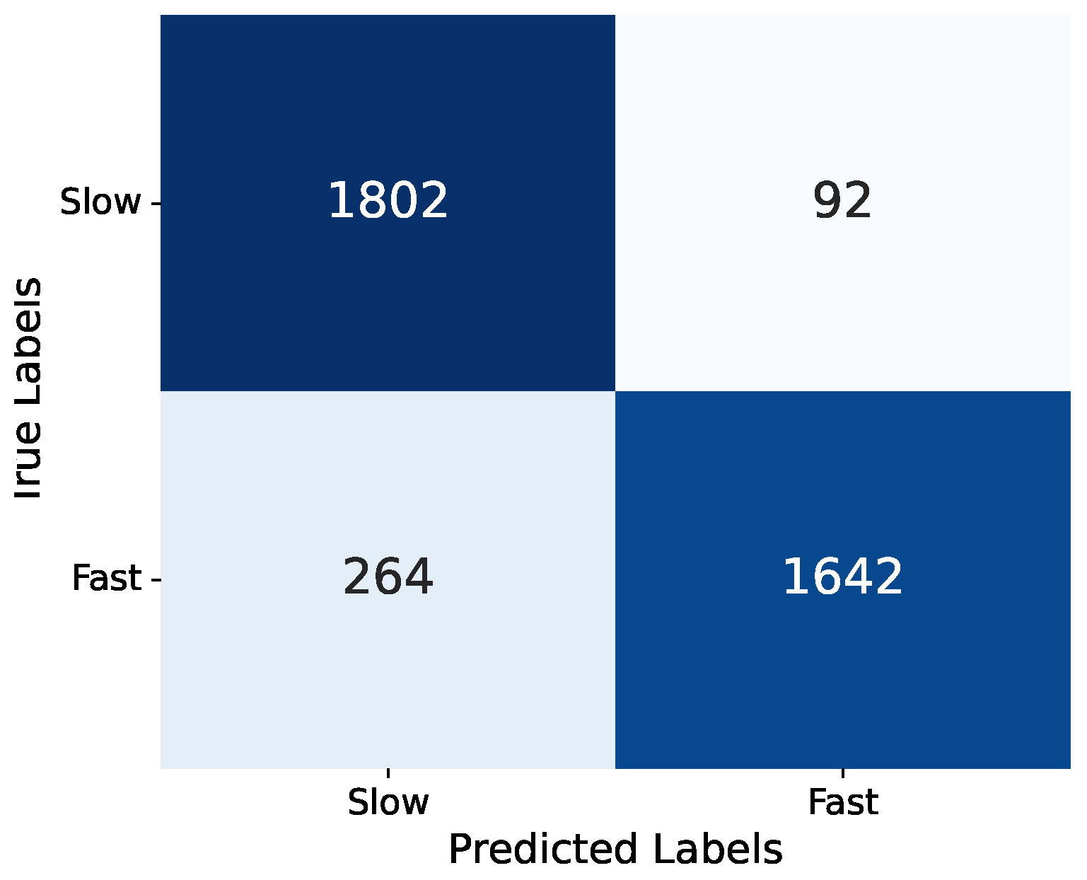
Figure 2.
The ROC plot demonstrates how the CNN model perform in distinguishing between fast/slow rotators samples across various thresholds, balancing true positive (TP) and false positive (FP) rates. The plot uses a logarithmic scale for the x-axis (FP rate), allowing for a more detailed view of the model’s performance at low FP rates
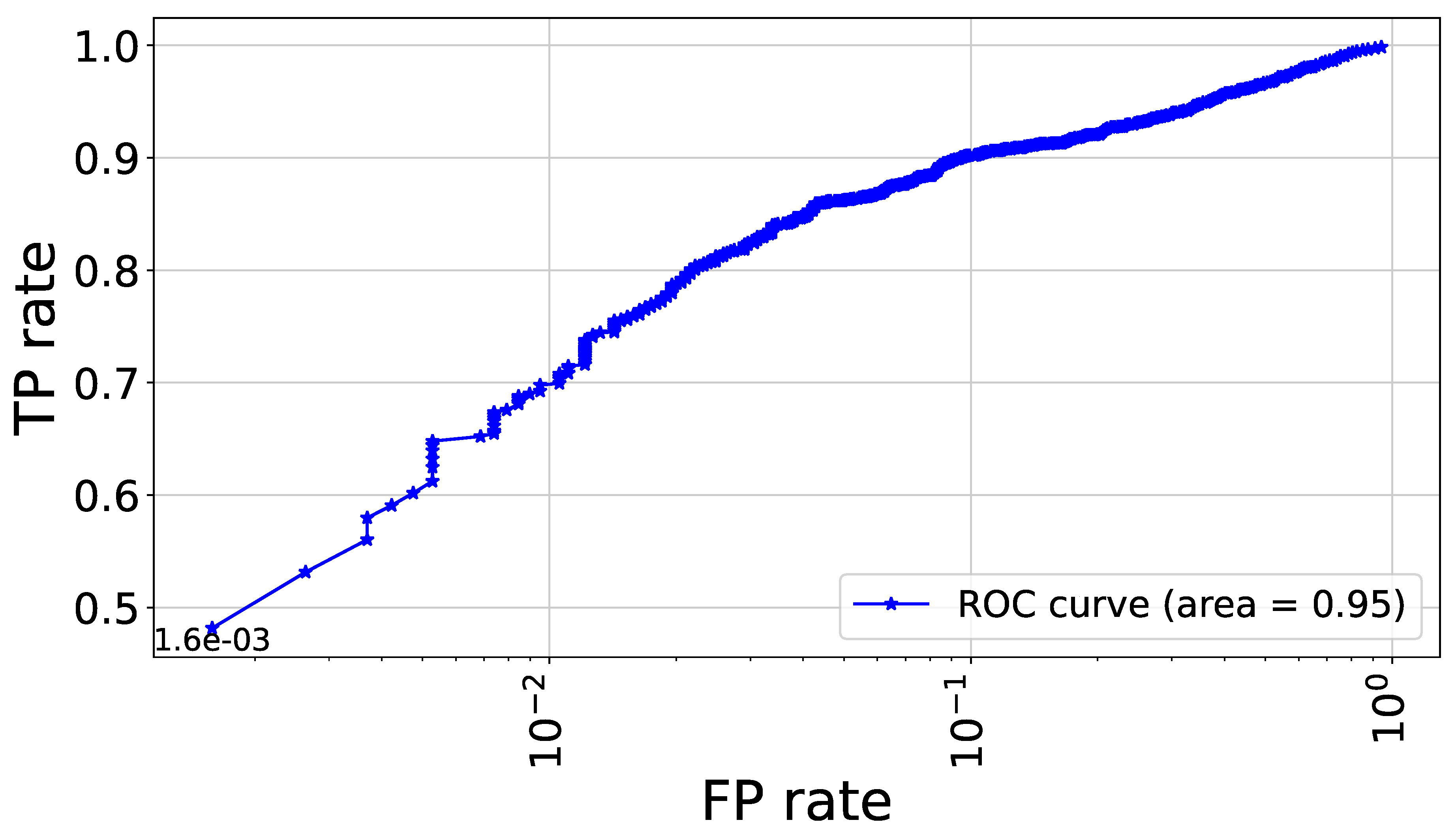
Figure 3.
This distribution plot compares the predictions made by the CNN model against the real test data. The x-axis represents the prediction probability from 0 to 1, while the y-axis shows the number of samples on a logarithmic scale.
Figure 3.
This distribution plot compares the predictions made by the CNN model against the real test data. The x-axis represents the prediction probability from 0 to 1, while the y-axis shows the number of samples on a logarithmic scale.
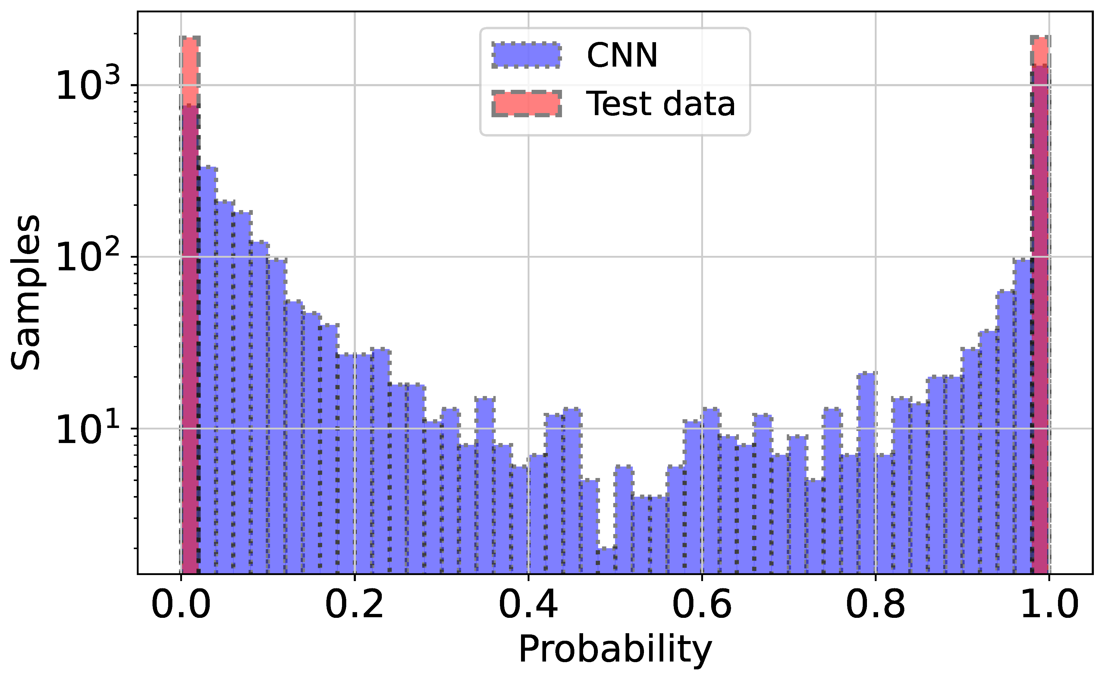
Figure 4.
These images presents distinct visualizations of false positive samples generated by the CNN model. Each visualization illustrates a different instance where the model mistakenly identified a slow rotator sample as fast one.
Figure 4.
These images presents distinct visualizations of false positive samples generated by the CNN model. Each visualization illustrates a different instance where the model mistakenly identified a slow rotator sample as fast one.
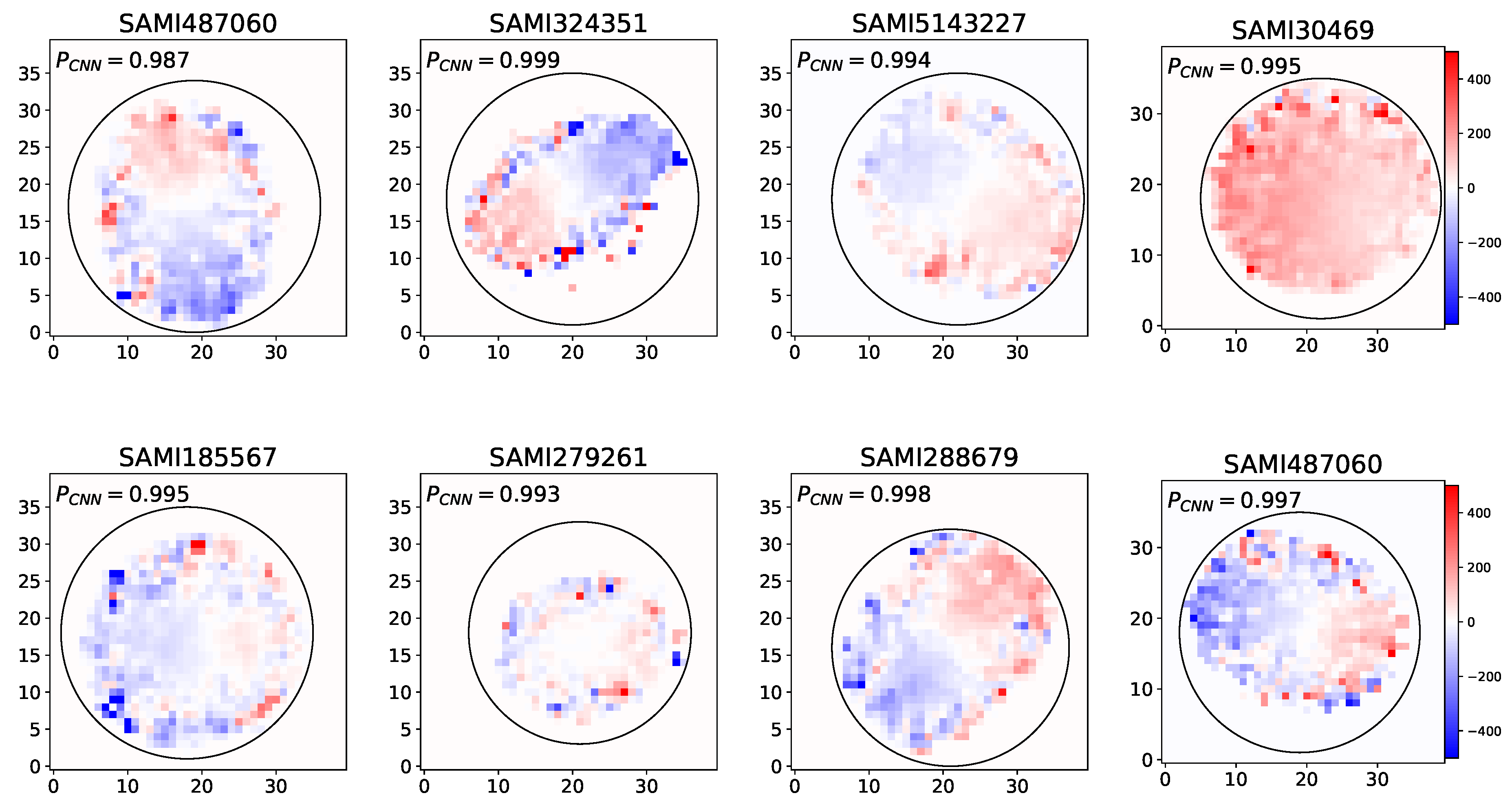
Figure 5.
These images presents distinct visualizations of false negative samples generated by the CNN model. Each visualization illustrates a different instance where the model mistakenly identified a fast rotator sample as slow one.
Figure 5.
These images presents distinct visualizations of false negative samples generated by the CNN model. Each visualization illustrates a different instance where the model mistakenly identified a fast rotator sample as slow one.
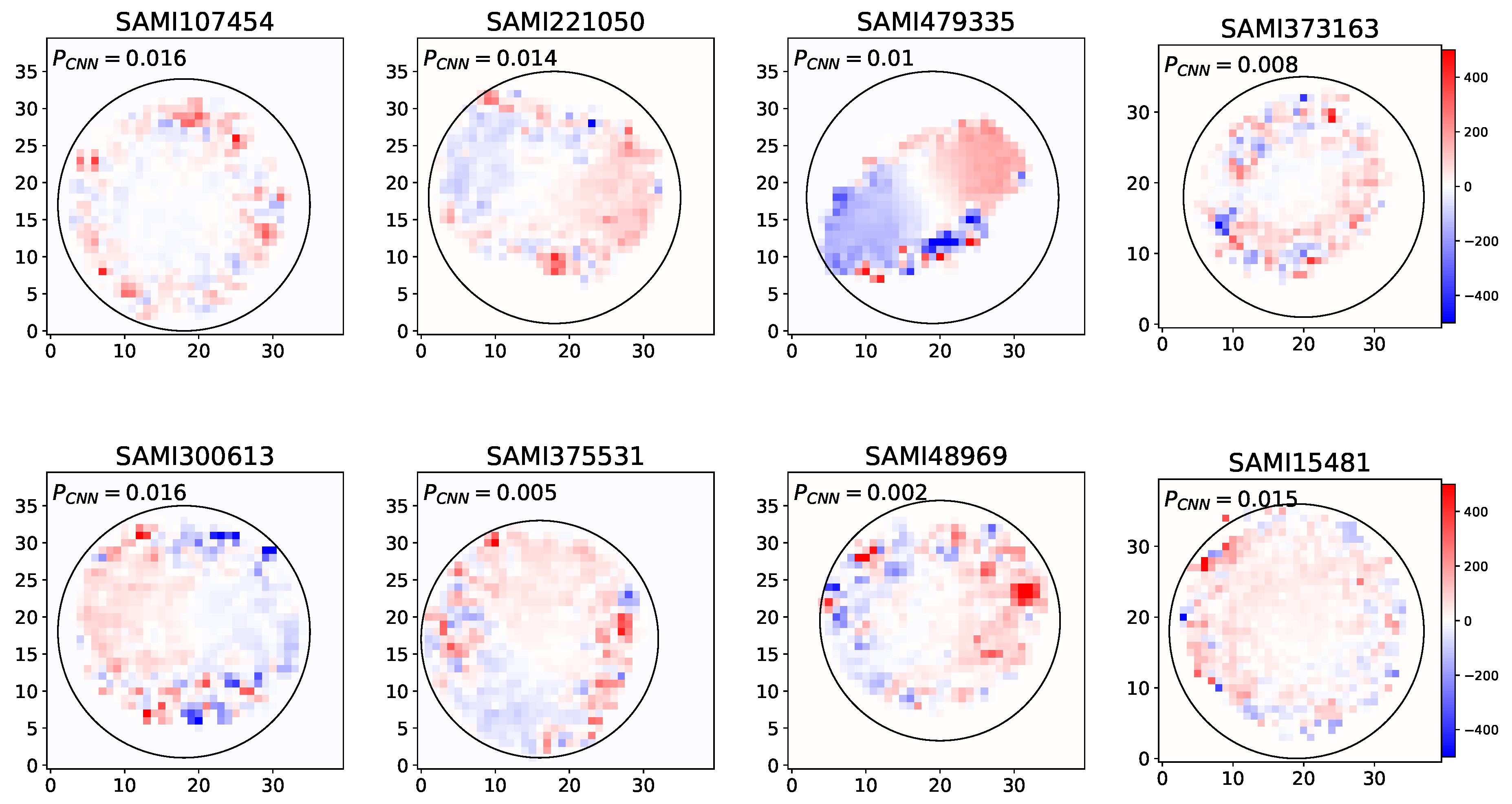
Figure 7.
These images showcases various visualizations of the unknown rotators samples that are face significant challenges in deriving -spin parameter. Our CNN model applied on these images and the probability predicted by CNN reported on the top of each image.
Figure 7.
These images showcases various visualizations of the unknown rotators samples that are face significant challenges in deriving -spin parameter. Our CNN model applied on these images and the probability predicted by CNN reported on the top of each image.
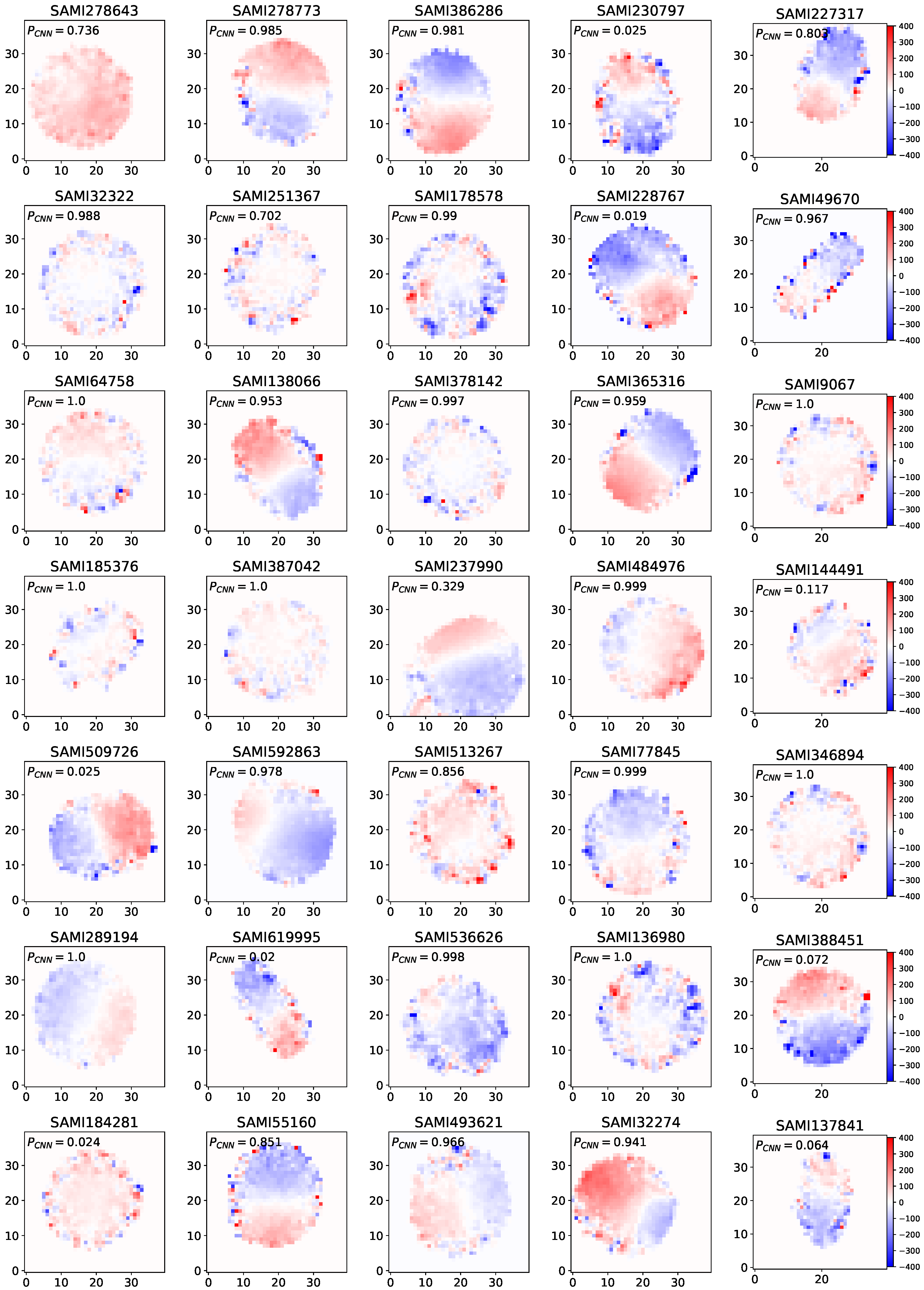
Figure 8.
Distribution of Moran’s I for slow and fast rotators, illustrating differences in spatial autocorrelation. Slow rotators (blue) exhibit a narrower distribution centered around lower values, while fast rotators (red) display a broader distribution at higher values.
Figure 8.
Distribution of Moran’s I for slow and fast rotators, illustrating differences in spatial autocorrelation. Slow rotators (blue) exhibit a narrower distribution centered around lower values, while fast rotators (red) display a broader distribution at higher values.
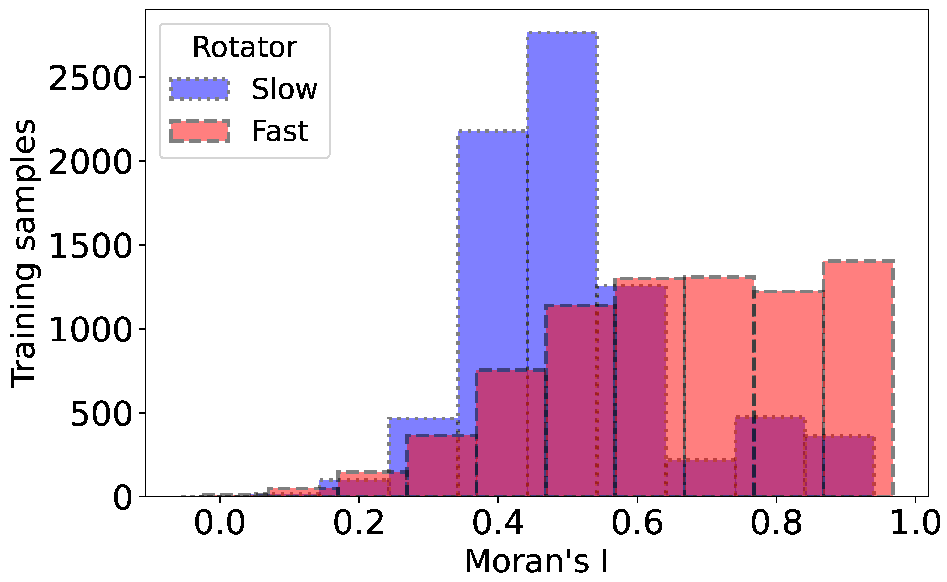
Figure 9.
Spatial autocorrelation of star velocities for two fast rotators from the SAMI dataset predicted by our CNN model. The central scatter plot shows the Moran scatter plot for each fast rotator, where the spatial lag of standardized velocity is plotted against the standardized star velocity. The top row presents spatial velocity maps, with red and blue regions representing higher and lower velocities, respectively. The right row displays the Integrated Gradients (IG) values for each pixel, where positive IG values contribute positively to the model’s decision.

Figure 10.
Spatial autocorrelation of star velocities for two slow rotators from the SAMI dataset. The central scatter plot shows the Moran scatter plot for each slow rotator, where the spatial lag of standardized velocity is plotted against the standardized star velocity. Lower Moran’s I values (0.385 and 0.180) suggest weaker spatial autocorrelation, indicating less coherent kinematic structures compared to the fast rotators analyzed in Figure 9. The bottom row displays the Integrated Gradients (IG) values for each pixel, highlighting that the majority of IG values are concentrated in regions with weaker spatial autocorrelation, further indicating less coherent kinematic structures in the slow rotators.
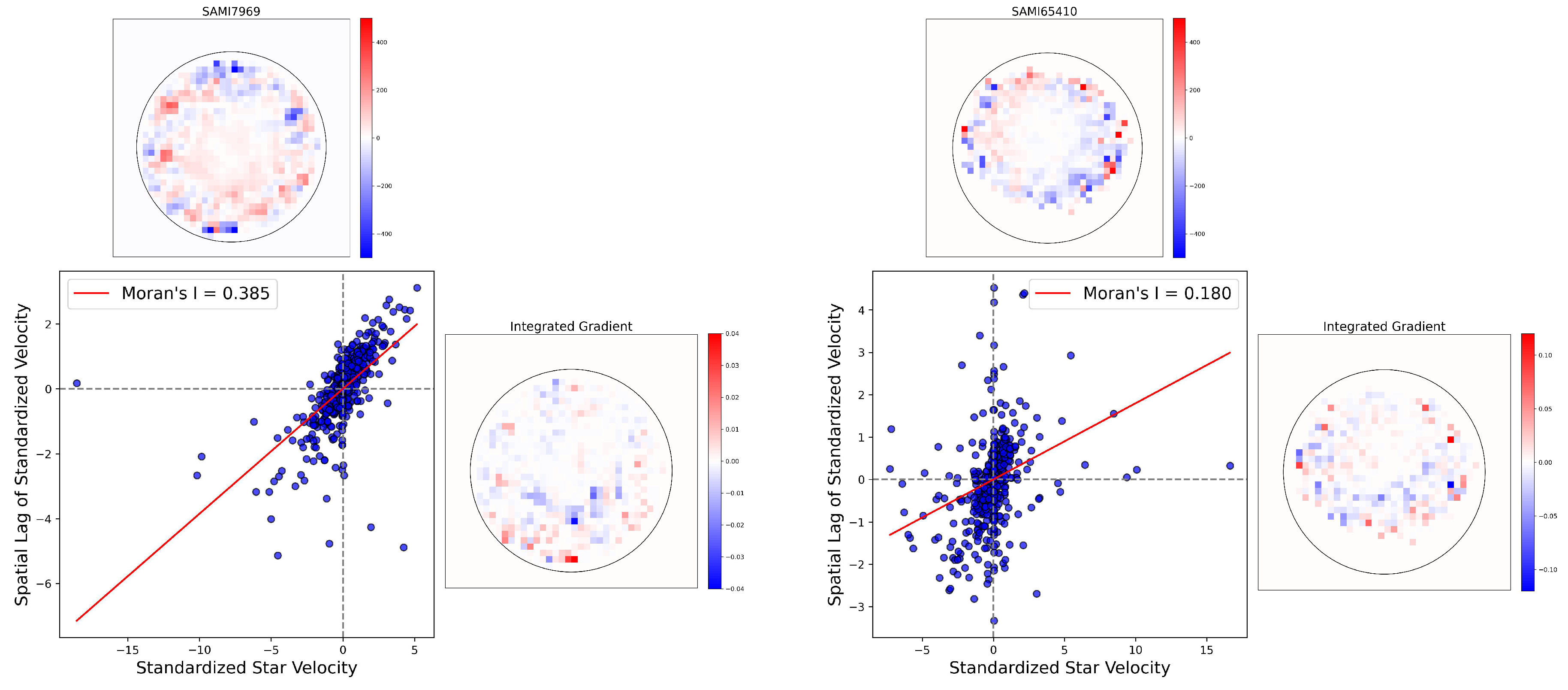

Table 1.
Summary of the Convolutional Neural Network (CNN) architecture, including layer types, output shapes, and parameter counts.
Table 1.
Summary of the Convolutional Neural Network (CNN) architecture, including layer types, output shapes, and parameter counts.
| Layer Type | Output Shape | Parameters |
|---|---|---|
| Conv2D | (None, 38, 38, 64) | 640 |
| MaxPooling2D | (None, 19, 19, 64) | 0 |
| BatchNormalization | (None, 19, 19, 64) | 256 |
| Conv2D | (None, 17, 17, 128) | 73,856 |
| MaxPooling2D | (None, 8, 8, 128) | 0 |
| BatchNormalization | (None, 8, 8, 128) | 512 |
| Conv2D | (None, 6, 6, 256) | 295,168 |
| MaxPooling2D | (None, 3, 3, 256) | 0 |
| BatchNormalization | (None, 3, 3, 256) | 1,024 |
| Flatten | (None, 2304) | 0 |
| Dense | (None, 96) | 221,280 |
| Dropout | (None, 96) | 0 |
| Dense | (None, 32) | 3,104 |
| Dropout | (None, 32) | 0 |
| Dense | (None, 1) | 33 |
Disclaimer/Publisher’s Note: The statements, opinions and data contained in all publications are solely those of the individual author(s) and contributor(s) and not of MDPI and/or the editor(s). MDPI and/or the editor(s) disclaim responsibility for any injury to people or property resulting from any ideas, methods, instructions or products referred to in the content. |
© 2025 by the authors. Licensee MDPI, Basel, Switzerland. This article is an open access article distributed under the terms and conditions of the Creative Commons Attribution (CC BY) license (http://creativecommons.org/licenses/by/4.0/).
Copyright: This open access article is published under a Creative Commons CC BY 4.0 license, which permit the free download, distribution, and reuse, provided that the author and preprint are cited in any reuse.


