Submitted:
03 March 2025
Posted:
04 March 2025
You are already at the latest version
Abstract
This study conducts a spatiotemporal analysis of groundwater data to map freshwater availability in Northern New Jersey, defining "freshwater coverage" as areas with groundwater specific conductance ≤750 µS/cm. Using ambient groundwater monitoring well data, salinity levels are predicted through geostatistical modeling, with specific conductance serving as a proxy for salinity. Kriging interpolation is employed to assess spatial variations in groundwater quality, utilizing optimal semivariogram models (e.g., Gaussian, Spherical, Exponential) for log-transformed data. Model accuracy is evaluated using metrics such as mean error (ME), mean standard error (MSE), root mean square error (RMSE), and root mean square standard error (RMSSE). The analysis reveals significant spatial and temporal variations in specific conductance, highlighting declining freshwater coverage, particularly in the Northeast region, which is most impacted by anthropogenic activities compared to the Northwest and Raritan regions. Overlaying highways and major roads on interpolation surfaces demonstrates a strong correlation between groundwater quality changes, changes in land use, and the widespread use of deicing salts on road networks. The findings highlights the decline in freshwater coverage and the influence of land use changes and road salt application on groundwater quality in Northern New Jersey.
Keywords:
spatiotemporal analysis
; kriging interpolation
; Northern New Jersey
; groundwater quality
; land use change
; specific conductance
; freshwater coverage
; salinity
1. Introduction
Water resource is critical to virtually every sector of human activities; from domestic water supply, agriculture, industrial use to other varied public water supply purposes [1,2,3,4]. Groundwater is a critical source of this water supply, as the United States utilized about 281 billion gallons of freshwater per day in 2015. About 30% of the total freshwater withdrawn was from groundwater sources. The same year, New Jersey withdrew about half a billion gallon of freshwater per day from groundwater supplies [1]. Since groundwater represents a vital component of the United States’ water supply, it is critical to ensure the long-term sustainability and quality of this valuable resource. Due to the huge demand, several studies across the United States are already observing the deteriorating quality of groundwater resources [4,5,6,7].
There are several controls driving the changes of groundwater quality. Lindsey et al. [8] studies of water chemical composition across the United States shows that increasing levels of Na and Cl ions serve as the main indicator for changes in groundwater chemistry. This was particularly observed in urbanized regions. In the United States' temperate regions, groundwater contamination poses a significant threat to water resources from varied sources. One major contamination source is urban runoff. During precipitation events, runoff carries pollution-ladened effluents into important water resources. Deicing salts applied on road surfaces during winter months infiltrate into groundwater, thereby compromising the water quality. Rural septic tank leaks are another source of contamination. Sewage waste from faulty septic systems contaminates groundwater, mostly impacting areas without centralized water and sewer infrastructure. The sewer system overflows carry every form of contaminant during heavy flooding events. Heavy storms and flooding cause combined sewer systems (such as found in New Jersey) to overflow, mixing with pollution-ladened runoff and seeping into groundwater. Aging sewer systems and inadequate infrastructure capacity often lead to overflows, leaks, and contamination. Generally, these combined sewer systems carry a mix of stormwater and sewage overflow during intense storms through manhole and line leaks, resulting in groundwater pollution [9].
Many studies in the United States have linked increased anthropogenic activities such as the use of deicing salt and rapid urbanization to continual deterioration of the groundwater quality [10,11,12]. Increasing groundwater contamination such as salinization has been observed to enhance the transport of contaminants from the land surfaces into the groundwater. Constituents like sodium ions from deicing salts application have been observed to release heavy metals from soil substrates into surface waters and groundwater [13,14]. The United States consumed about 58 million metric tons of salt in 2019, with about 43% of this salt (which are mainly in the form of sodium chloride) reported to be applied to Highway cleaning [11,15]. Roads in the urban regions of northern New Jersey consume about a third of a million metric tons of deicing salt annually. Reports from the New Jersey Department of Transportation (NJ DOT) reveal that New Jersey used about 10,000 kg of NaCl for every lane kilometer (0.621 mile) in 2017 [16]. The northern New Jersey's region covers about 18,000 miles of urban public roads [17]. This is the key reason for its much-needed application of deicing salt during wintry conditions.
Specific conductance serves as a valuable proxy for evaluating groundwater quality, especially in areas impacted by runoff from urbanization and agricultural activities, where increased levels of conductance indicate eutrophication and pollution [18]. Specific conductance indicates a broad insight into the levels of water quality, representing the various contaminant levels available in the water. Specific conductance values are largely used for extrapolating salinity levels in water [19,20,21]. Cartwright et al. [22] indicates that Specific conductance can be applied as a proxy technique for establishing salinity. The metric unit for specific conductance of water is in microsiemens per centimeter (μS/cm) and this provides a measure of salinity for various water sources; ocean water (55,000 μS/cm), distilled water (0.5 – 3.0 μS/cm), melted snow (2 – 24 μS/cm), portable water (30 – 1500 μS/cm), tap water (50 – 800 μS/cm) [23]. A level of 150 – 500 μS/cm is usually desired for general purposes [24,25]. United States Salinity Laboratory [26] classifies salinity with respect to specific conductance, as low salinity (100 – 250 μS/cm), medium salinity (250 – 750 μS/cm), high salinity (750 – 2250 μS/cm), and very high salinity (> 2250 μS/cm).
Increases in salinity have been observed in northern New Jersey, as several anthropogenic sources (such as the use of deicing salt) have been ascertained to influence the quality of water resources [12,27]. In recent times, rapid urbanization that occurred in New Jersey has seen an increase of about 23% during the short period of 1995 – 2000, compared to observation from 1986 to 1995. These land use modifications were observed all across the state of New Jersey, with Morris, Sussex, and Somerset counties suffering the most intense loss of forested areas in northern New Jersey [28].
Continuous assessment of groundwater resources is essential to provide decision-makers and stakeholders with critical information on freshwater availability, ensuring it meets the growing demand for supply. However, to ensure the public can easily understand the status of their groundwater quality, there is a need to present this information in a simplified and accessible manner. Such clear and concise data is vital during community engagement meetings, enabling informed discussions and the development of sustainable solutions to address water quality challenges. Visualizing these data would provide a better understanding of the current status and trend of the groundwater quality. It is necessary to know whether a particular region is heading in the right direction in terms of work that needs to be done to ensure continual availability of freshwater.
The power of visualization in GIS can be adapted to provide a characterization of groundwater quality across the study area. The use of GIS would provide spatial variability of the water quality in the region across varied land uses. This study focuses on the use of geospatial analysis to estimate the specific conductance as a measure of the groundwater quality in watersheds across northern New Jersey. The study uses GIS to provide spatial and temporal variability in specific conductance in the various WMAs, considering land use and Highways in the region. The study provides a mapped-out correlation between land use, Highways and spatial variability of specific conductance across different WMAs in northern New Jersey. The total extent of areas with available freshwater across northern New Jersey are outlined using freshwater metrics as indicated by United States Salinity Laboratory Staff [26]. The study methodology provides an estimate of salinity as an indication of freshwater in areas without measured specific conductance and indicates the various levels of water quality in the WMAs in the region. The aim is to develop a geostatistical model to predict salinity levels as a measure of groundwater quality, using specific conductance values already measured from specific locations to determine the areal coverage of freshwater. The analysis would reveal the salinity concentration distribution over time and indicate changes occurring over that period. A simple data visualization of the effect of deicing salts on groundwater across the region is provided. The kriging interpolation method in GIS is used to develop the geostatistical model which provides a representation of salinity in the area. This technique quantifies salinity in the entire region using data from measured locations to estimate data in unmeasured locations. Several studies have applied varied spatial interpolation techniques in assessing water quality using various parameters as indicators of suitability or state of quality [29,30,31,32,33]. Research indicates that the Kriging interpolation technique outperforms other interpolation methods [34,35,36]. This technique is known for its ability to generate accurate estimates at unsampled points using values from neighboring measured points [29,37], while minimizing error [38]. It is also known to provide a more accurate distribution of parameters across geographical areas [39]. Currently, there is no spatial analysis study that provides a spatial distribution of water quality across northern New Jersey, nor any research identifying areas in the region with available freshwater. Therefore, this study provides decision makers and concerned individuals with valuable insights on the current status and availability of freshwater, as well as potential changes in groundwater quality overtime in northern New Jersey.
1.1. Study Area
Geologically, New Jersey is partitioned into two parts by a fall line, the north and south parts. The non – coastal plains region is the north part of the fall line while the coastal plains region is south of the fall line. This study is focused on New Jersey non - coastal plains water region which is also referred to as the northern New Jersey water region. Three water regions are located in northern New Jersey, the Northwest, Northeast, and Raritan water regions. There are eleven WMAs in the three regions; Upper Delaware (WMA - 1), Wallkill (WMA - 2), Pompton, Wanaque, Ramapo (WMA - 3), Lower Passaic and Saddle (WMA - 4), Hackensack and Pascack (WMA - 5), Upper Passaic, Whippany, and Rockaway (WMA - 6), Arthur Kill (WMA - 7), North and South Branch Raritan (WMA - 8), Lower Raritan, South River and Lawrence (WMA - 9), Milestone (WMA - 10), and Central Delaware [40,41] (Figure 1a). The study area is characterized by a unique bedrock geology. The physiographic provinces include, “the Valley and Ridge, Highlands, and Piedmont provinces.” [41]. Detailed literature on the bedrock geology of northern New Jersey is found in studies by Dalton et al. [42], Drake et al. [43] and NJDEP [44]. Northern New Jersey comprises primarily of old consolidated geological units covering about 3,116 square miles in area and makes up two-fifths of New Jersey State [41,45]. The area covers 12 counties of New Jersey; Sussex, Passaic, Bergen, Hudson, Essex, Morris, Warren, Hunterdon, Somerset, Union, and parts of Middlesex and Mercer [45]. The fall line cuts through WMAs 9, 10 and 11 (Lower Raritan, Millstone and Central Delaware WMAs), thereby placing some of these WMAs’ groundwater wells in the south part of the fall. In this study, all the wells within WMAs 9, 10 and 11 in both the north and south parts, were analyzed as part of the northern New Jersey region. This was done to harness as much data as possible.
The northern New Jersey region comprises agricultural, undeveloped, and urban land use (Figure 1b). The Northwest water region has the largest agricultural area. The Northeast water region has no agricultural land use area, and it is the most urbanized water region. The Land use areal markings of the data used in this study were obtained from “1986 and 1995 land-use geospatial mapping” [46].
2. Methods
2.1. Data Collection
To spatially assess the groundwater quality of the watersheds of northern New Jersey, available data were analyzed and mapped out. The data was obtained from the achieves of the New Jersey Ambient Groundwater Quality Monitoring Network (AGWQMN) database, containing hydrogeological data from shallow wells across New Jersey. The data furnish information on “nonpoint-source contaminants” impacting the groundwater. The New Jersey AGWQMN data used in this study cover four sampling time cycles (cycle 1: 1999 – 2004, cycle 2: 2004 – 2008, cycle 3: 2009 – 2013 and cycle 4: 2014 – 2016). Two hundred and ninety-five (295) well observations from the water regions in northern New Jersey were obtained for this study. Groundwater wells used in this study were completed in unconfined aquifers to enhance insights on groundwater contamination from the near surface [41]. This study was evaluated based on four sampling cycles. Cycles 1, 2, and 3 included data from 76, 77, and 77 wells, respectively, covering all three land use types: agricultural, undeveloped, and urban. Cycle 4 was split into Cycle 4 and 'Adjusted Cycle 4,' with data from 65 and 77 wells, respectively. Unlike the earlier cycles, Cycle 4 excluded data from 12 wells of undeveloped land use area. The 'Adjusted Cycle 4' combines well data from Cycle 4 with a set of "well data from the undeveloped land use" taken from Cycle 3. This adjustment assumes a scenario where the well data from the undeveloped land use during the Cycle 3 sampling period remained unchanged and were observed again in Cycle 4. As a result, Cycle 4 does not include undeveloped land use well data, while 'Adjusted Cycle 4' incorporates well data from the undeveloped land use area.
The collected data were cleaned and prepared for analysis using R, an analytical software [47], along with QGIS [48] and ArcGIS [49] for geospatial analysis in this study. The choice of the geochemical parameter ‘specific conductance’ for the spatial modeling and estimation of the groundwater quality was based on well documented literature [18,22].
The analysis process is computationally intensive, following a workflow (Figure 2) to meet the goal of the study. The process can be divided into four major tasks: (1) data collection and processing – exploratory data analysis, (2) develop/fit semivariogram model, (3) Cross – validation and (4) Kriging interpolation. The kriged predictions were then mapped out and freshwater areas calculated.
2.2. Data Analysis
This study uses kriging interpolation to provide a clear understanding of the level of salinity and the overall quality of the groundwater in Northern New Jersey’s 11 WMAs, over a time period. Specific conductance values, which are a measure of salinity, were used to spatially evaluate the groundwater quality in the WMAs across the region, indicating varied water quality distribution over the several water sampling cycles.
2.2.1. Kriging Interpolation
Kriging is a geostatistical interpolation technique utilized for predicting values at unsampled locations based on measurements from known locations. Kriging interpolation is distinguished by its ability to assess estimation errors and to quantify uncertainty in the interpolated surfaces. Studies have indicated that Kriging provides more accurate predictions compared to other deterministic and stochastic methods, making it a preferred technique for spatial analysis [35]. Kriging interpolation is one of the most efficient and widely applied techniques in geospatial analysis of environmental variables [2,31,32,33,50]. The interpolation methods include universal kriging (UK), simple kriging (SK), ordinary kriging (OK), and cokriging (CK) [51,52,53]. Among these, ordinary kriging is widely recognized, and it is applied in this study due to its simplicity, minimal assumptions, and superior prediction accuracy relative to other kriging variants [32,54]. Ordinary kriging can be used for the interpolation of spatial distribution with trend [53]. This variant is particularly suitable when the primary objective is to produce a prediction map. In addition to the prediction map, kriging interpolation also produces uncertainty, which makes it a more reliable interpolation techniques for prediction of unknown points [55].
2.2.2. Exploratory Data Analysis
Exploratory Data Analysis is aimed at analyzing the statistical and spatial attributes of the data. The data is explored to indicate the distribution patterns, data uniformity and trends. A plot of histogram is used to determine the normality of the data distribution. In occasions when the data is not normally distributed as commonly found among environmental data, the data undergoes transformation (commonly applied is the log transformation) to make the data log-normal [32].
It is important to note that for a spatial distribution of data to undergo ordinary kriging interpolation, the data has to meet the assumption of normality and stationarity (constant variance), to provide accurate predictions. Data transformation is a quick fix to the issue of normality assumption, and also an applicable solution during instances when the data fails to meet the stationarity assumption. The Log transformation of skewed data sets during the exploratory data analysis draws the data closer to normality and satisfaction of the stationarity assumptions [54]. In order to minimize the deviation from the assumptions and/or avoid the violation of these assumptions, it is therefore important for skewed data to be transformed. The primary basis for analyzing the trend during geostatistical interpolation is to satisfy stationarity assumptions [53]. Since the log transformation of the data fixes the issue of normality assumption and satisfaction of stationarity assumption, it is inferred that there is no trend in the data distribution and the stationarity assumption is satisfied. Johnston et al. [53] and Chiu [56] indicate that the Voronoi map provides a deeper understanding of the distribution patterns of points and examines the trend and stationarity assumption.
2.2.3. Experimental Semivariogram
The Kriging method is based on the principle of spatial autocorrelation, which is central to geostatistical applications. To analyze the spatial distribution of data values and their parameters, semivariograms serve as a key descriptive tool. Spatial dependence between measured points is determined by calculating semivariance, which considers the distances between these points. The use of plotted semi-variogram indicates the relationship between the lag distance and the semi-variance, the variogram evaluates the sampling errors [35]. The lag distance refers to the separation between measurements of a given property. Typically, the semivariance values increase with decreasing lag distance, indicating stronger spatial autocorrelation [57]. Various models, such as Gaussian, Spherical, and Exponential, are then applied to fit the semivariogram and identify the most appropriate model for generating optimal interpolation weights [52]. Kriging is a highly versatile interpolation method that can produce both exact and smooth surfaces. It supports a range of output surfaces, including predictions, standard errors of prediction, and probabilities. The Kriging technique facilitates optimal, unbiased estimation of regionalized variables at unsampled locations by leveraging the properties of semivariograms and initial data points [35].
In geostatistics, the semivariance function is utilized to calculate and interpret spatial correlation patterns, particularly when the sampled data values follow a normal distribution, and the skewness falls within the range of -1 to +1 [35]. Semivariogram analysis is a key technique for visually indicating spatial correlations among neighboring data points. A semivariogram plot is generated by calculating semivariance values across various lags. The models—circular, spherical, exponential, and Gaussian—furnish insights into the spatial structure for Kriging interpolation. Key characteristics of the semivariogram (as shown in Figure 3) include range (a), sill (C0 + C), and nugget effect (C0) [32]. The nugget refers to the Y-intercept of the semivariogram model, while the sill is the semivariogram value at which the model stabilizes or levels off [58]. The selection of the appropriate lag size is calculated based on multiplying the number of lags times the lag size, which should be ‘half the farthest distance between any point’ [53] or about the ‘whole farthest distance between any point,’ as applied in this study. However, the range of the fitted semivariogram model is highly influenced by the lag size [53]. The equations below indicate how the semi-variance function, γ(h) and unmeasured values at a given distance, h are calculated [59,60]:
where: γ(h) = semi variance value at lag distance, h,
Z = regionalized variable,
Z () = measured value at point, ,
Z( = measured value at point, (,
n = number of pairs separated by distance, h.
where: Z (Xo) = estimate of unknown true value,
λi = weighted coefficient, n = number of neighboring observations.
2.2.4. Cross-Validation
Experimental semivariogram values were tested for different types of semivariogram models (Circular, Spherical, Exponential, and Gaussian) and were evaluated to identify the most suitable model for salinity estimation. The predictive performance of each fitted model is assessed using spatial cross-validation metrics. Various error metrics are calculated, these include “mean error (ME), mean square error (MSE), root mean square error (RMSE), average standard error (ASE), and root mean square standardized error (RMSSE).” Ideally, if the predictions are unbiased, the ME should be close to zero, though this statistical inference has limitations, as it is scale-dependent and does not fully capture inaccuracies in the variogram. Therefore, MSE, which builds on ME by squaring the errors, is often used, with an ideal MSE value approaching zero, indicating an accurate model [32].
As MSE should be close to zero to ensure prediction accuracy, RMSE also should be as minimal as possible [29,51,53]. If RMSE aligns with ASE and their values are close, it indicates that the prediction errors were correctly estimated. However, if RMSE value is smaller than ASE, the prediction is overestimated, while an RMSE greater than ASE suggests that the prediction is underestimated. Similarly, RMSSE values close to one indicate correct estimation of variability. Values above one suggests underestimation, while values below one imply overestimation of variability. After completing the cross-validation process, Kriging-generated maps were produced, providing a visual depiction of the spatial distribution of groundwater quality [31].
2.2.5. Kriging Map Generation
After cross-validation, the estimated kriging values of the groundwater for all sampling cycles are mapped out, and the maps are graded according to the level of salinity as indicated by USSL [26]. Available freshwater quality of the WMAs in northern New Jersey is evaluated, as the study uses 750 μS/cm value of specific conductance as the threshold for salinity, and any value higher than 750 μS/cm is not considered to be freshwater. Total area with available freshwater is assessed for the four sampling cycle periods – indicating the freshwater coverage and changes in freshwater per the study area coverage over time. Thereafter, layers of WMAs, major roads and highways in northern New Jersey are overlaid on the generated kriging maps and are assessed to observe their relationship and influences in the varied levels of groundwater quality across the region.
2.2.6. Limitation
It is important to recognize that actual spatial variations can significantly differ from the values predicted by spatial interpolation, which may present limitations in the Kriging method, particularly when data is sparse or unevenly distributed. Therefore, understanding both the number of data points and the geographical coverage of the region is crucial. The kriging interpolations are executed based on two primary assumptions: the stationarity of the target variable and its conformity to a normal distribution. Nevertheless, environmental data often deviate from these assumptions, exhibiting complex patterns and distributions. In response to this challenge, this study undertakes a data transformation to attempt to satisfy the assumptions [52]. One of the most challenging aspects in such cases is accurately estimating the variogram model, which becomes more difficult with fewer data points [31]. Additionally, ME statistical metric used for evaluating prediction performance has notable limitations, as it is scale-dependent and does not fully account for variogram inaccuracies. To address this, MSE which builds on ME by squaring the errors, is often used, with an ideal MSE value close to zero indicating an accurate model [32].
3. Results and Discussion
Rapid urbanization and industrialization across the world are degrading freshwater resources, as anthropogenic activities continue to alter land use and introduce contaminants into the environment. Kriging interpolation provides visual insight into the state of groundwater quality, clearly indicating the freshwater coverage in any region. Groundwater specific conductance value of 750 μS/cm or lesser is used as a marker for freshwater.
3.1. Exploratory Data Analysis
First an exploratory analysis process, which is crucial for spatial relationship of the data and appropriate selection of model is performed for all sampling cycles. The histogram in Figure 4a reveals that the groundwater data is highly skewed, does not have a bell-shape, and therefore, unsuitable for kriging interpolation. Figure 5a shows the use of normal Q-Q plots to provide an analysis of univariate normality. Data for all the sampling cycles indicated to be asymmetric, and most of the points are drifting from the line of best fit. The Normal Q-Q plots and histograms indicate that the data is not normally distributed and needs to be transformed before further analysis. After the log transformation of the data, the histograms and normal Q-Q plots show that the distributions are close to normal (Figure 4b and 5b). The log normal statistics (Table 1) reveal close values of the means and medians, the skewness is near zero (falls within the range of -1 to +1), and the kurtosis values are close to 3. These statistics of the log transformed data show that the data are normalized and meet at least one of the assumptions for kriging interpolation – the normality assumption.
This log transformation ensures equal variance across the data, thereby possibly satisfying the other assumption (stationarity). The Voronoi maps (Figure 6) of the transformed data provide a visual and qualitative assessment of trends, as well as an analysis of the spatial variability of the data [56,61]. The Voronoi maps indicate that there is no clear existence of linear global trend in the data and provide satisfaction towards the stationarity assumption. Figure 6 has an Illustration of trend occurrence in spatial data, as the Voronoi map shows the occurrence of a visually noticeable linear trend.
The removal of trend from data during kriging interpolation should be based on a proper justification [53]. When spatial coordinates indicate an observed or suggested trend in the data [49], as seen in this study where land use significantly influences water quality, it would make sense to retain the trend.
Furthermore, Jarmołowski et al. [62], in their study on "drawbacks of trend removal during kriging interpolation," provide rationales for retaining trends in heterogeneous spatial data, such as data significantly influenced by land use type. Their rationales include (1) maintaining the trend of a spatial data can help capture the underlying spatial structure more effectively, (2) unbiasedness of ordinary kriging must be ensured, and retaining the global trend can help achieve this by providing a more stable reference for predictions, (3) In scenarios where data is sparse, keeping the trend can provide a more reliable framework for interpolation. Following the logarithmic transformation of the data in this study, a deliberate decision was made to refrain from detrending the data. This approach was adopted to minimize complexity and ensure reliability of the results. Considering that groundwater quality in this study is influenced by varied land use patterns and non-point pollution sources, which are spatially heterogeneous and linked to specific locations, detrending may mask these spatial relationships. Therefore, not removing the trend (if any) in the data is justified. This study relies on the predictive performance metrics of the kriging interpolation to measure the performance of the kriging interpolation.
3.2. Experimental Semi-Variogram
The plotted semi-variograms (Figure 7) show the relationship between the lag distance and the semi-variance. The variogram evaluates the sampling errors across the spatial data for all the sampling cycles. The selection of the appropriate lag size for this study is evaluated based on multiplying the number of lags by the lag size, which is about the ‘whole farthest distance between any point.’ This is in contrast with the approach suggested by Johnston et al. [53], that the ‘golden rule’ for the selection of lag size is based on half of the “farthest distance between any points.” Applying ‘about the whole distance’ instead of ‘half the distance’ in this study (410,000 – 450,000 meters) showed to support more prediction accuracy as reflected in the prediction performance metrics (MSE, RSME, etc.). Using the established lag size and lag number, the experimental semivariograms are fitted for various types of semivariogram models (Circular, Spherical, Exponential, and Gaussian). Nugget and sill parameters were calculated using the Geostatistical Analyst tool for each model, and no adjustments were deemed necessary. The nugget represents the Y-intercept of the semivariogram model, while the sill refers to the semivariogram value at which the model stabilizes or levels off [58]. The gaussian model showed to be the best fit for all the sampling cycles, and the statistics metrics (Table 2) were used to evaluate the performance of each model.
3.3. Cross-Validation
Cross-Validation facilitates model evaluation by estimating prediction accuracy at unmeasured locations, with ideal model performance characterized by near zero MSE, minimal RMSE, standardized RMSE near 1 and equivalent values of RMSE and ASE. Table 2 shows the model performance metrics for all the sampling cycles, indicating that the selected models are of optimal performance level. The metrics show that RMSE and ASE have equivalent values, both close to zero, while MSE and RMSSE are near 1, suggesting that the model was neither overestimated nor underestimated.
3.4. Kriging Map Generation
After evaluating the model performance metrics, the estimated kriging values of specific conductance of the groundwater for all sampling cycles are mapped out, and the maps are graded according to the level of salinity as indicated by USSL [26]. The kriging interpolation produced a raster map of salinity indicating various levels of groundwater quality. The kriging interpolation provided a salinity distribution representing the groundwater quality of northern New Jersey WMAs, from sampling cycling 1 to 4, plus sampling cycle 4 – adjusted. This study uses 750 μS/cm value of specific conductance as the threshold for salinity, and any water with salinity higher than 750 μS/cm is not considered to be freshwater. The kriged maps (Figure 9) provide an insightful visualization of the groundwater quality various across the land use types in the study area. The legend of the kriged map shows color patterns from blue to red, with blue indicating the lowest levels (best water quality), and red the highest levels of salinity. Several layers were overlaid on the kriged surface to provide better understanding with varied influences from anthropogenic activities. These layers include highways, all major roads, sampling points, and 11 WMAs of northern New Jersey.
The major highway and WMA layers are overlaid onto the land use layer map (Figure 1b) to visually illustrate the region’s urbanized area and their relationship with varied levels of groundwater quality. The highway overlay suggests potential contributions to pollution, from major highways, likely from plying vehicle and the application of deicing salts during icy and snowy conditions. The land use map revealed that the Northeast water region is the most urbanized, followed by Raritan water region. The Northwest region has the most coverage of undeveloped and agricultural land use areas. The urbanized Northeast region is characterized by a dense network of roads, including highways and major roads. When these roads were overlaid on the kriged map, they nearly covered the entire Northeast region, making it difficult to clearly recognize the patterns (colors) on the kriged map beneath (as shown in Figure 8). This high road density highlights the prevalence of impermeable surfaces, which serve as areas where contaminants accumulate. During precipitation events, runoff carries these contaminants to areas not originally associated with such pollution, exacerbating water quality issues linked to non-point pollution sources. Also, the larger the impervious surfaces (such as roads), the larger the volume of deicing salts applied during snowy and icy conditions, indicating that areas with heavily dense roads will have their water resources more impacted by the applied deicing salts. The overlaid sampling points reveal that the sampling points are sparse and evenly distributed, covering an area of about 3,400 square miles. The sampling points are considered sparse because certain WMAs have very few points such as WMA 03 – Pompton WMA in the Northeast region. This WMA has only two wells (in an area of about 240 square miles) for monitoring the ambient water quality. The Pompton WMA is mostly undeveloped forested area (as indicated in the land use map), that is observed to have better water quality relative to other land use areas. That the location of WMA is mostly forested area, may be one reason the AGWQMN monitoring network has only two wells. However, with the rapid urbanization occurring as indicated by Lathrop [28], more wells may need to be developed in such regions so as to capture any possible water quality deterioration that could result from anthropogenic activities. The rapid change in land use towards urbanization could cause the groundwater to deteriorate in quality.
Figure 9 provides a kriging interpolation prediction map of groundwater quality in northern New Jersey across four ambient groundwater sampling cycles (1999 – 2004, 2004 – 2008, 2009 – 2013 and 2014 – 2016). The map provides a prediction of specific conductance values, which serves as an indicator of salinity levels, and an overall metric for the quality of the groundwater in the region. The map aims to quantify the coverage of available freshwater in northern New Jersey, while also highlighting the WMAs that are exhibiting increasing salinity and/or characterized as ‘non-freshwater’. On the kriged map, colors ranging from blue to yellow indicate freshwater. The yellow color indicates a specific conductance value of 750 μS/cm, which serves as the threshold for freshwater in this study. In contrast, brownish or reddish areas on the kriged map indicate high salinity levels, reflecting poor groundwater quality. As shown in Figure 9a, the spatial distribution of salinity reveals a distinct pattern. The Northwest water region, predominantly blue, exhibits low salinity, while the Raritan region shows low to moderate salinity (ranging from green to yellow). In contrast, the Northeast region displays the highest salinity, predominantly red, during the first sampling cycle. The distinctive levels of kriged salinity in the study area is highly associated with the varied land use of the region. The most urbanized area exhibits the worst water quality, while regions with less urbanization and more undeveloped land use showed better water quality with respect to salinity. This expression of salinity is also associated with the density of road network across the study area. The Northeast water region, which has the most densely concentrated road network, exhibited the highest salinity. This is likely attributed to the widespread use of deicing salts, facilitated by the region's large areas of impermeable surfaces [5,63] Aside from the influences of deicing salts, various studies [5,63,64] have revealed that wastewater contributes to increasing salt ion levels in water resources. This heavily urbanized Northeast water region is serviced by old sewer collection systems (combined sewer system) that combine sanitary sewer waste and stormwater in one line. During heavy storm events, overflow through the manholes of these combine sewer systems could bring up heavy salt-laden wastewater to the subsurface, thereby infiltrating into the groundwater system and contaminating water resources.
Figure 9b illustrates the kriging prediction for the second sampling cycle. The spatial distribution of salinity across the study area closely resembles that of the first sampling cycle, with the northeast water region again showing the highest salinity. This is consistent with the region's heavy urbanization, as previously discussed. However, the kriged map reveals an overall increase in salinity across all water regions. Notably, areas that were previously blue, green, or even brown color in the first sampling cycle now exhibit more yellow coloration, indicating fluctuating salinity levels across the region. The Northwest region shows more of the yellow color in this sampling cycle. The increasing salinity in this region may be attributed to use of agricultural fertilizer, an activity that is prominent in the Northwest region’s land use. Kaushal et al. [5] and Marghade et al. [64] indicate that agrochemicals contribute to freshwater salinization, however, the Northwest region still has a good coverage of freshwater compared to other water regions.
During the third sampling cycle, the kriged map (Figure 9c) reveals that the spatial distribution of the salinity across the study area remains similar to those of the two previous sampling cycles. The Northeast water region has a larger coverage of poor groundwater quality compared to other water regions in northern New Jersey. The water quality in the water regions were chiefly influenced by their varied land use activities. There is one visually observable difference in sampling cycle 3 within the Northwest region. In this region, there appears to be a reduction in salinity, as indicated by areas that were yellow during cycle 2, now turning green in cycle 3, suggesting a decrease in salinity. For instance, an area with a specific conductance value of 750 µS/cm (yellow) during cycle 2 may now measure 700 µS/cm (green) in cycle 3. While this change demonstrates a decline in salinity, it does not necessarily imply an increase in freshwater coverage. This is because, from the cycle 2 to cycle 3, any area with specific conductance value of 750 µS/cm or less is considered to be freshwater. Thus, the observed reduction in salinity is not accompanied by clear evidence of expanded freshwater availability in the region. The reduced salinity in the Northwest region could be attributed to adequate freshwater flushing in the groundwater system, as reported by Rossi et al. [63] and Sun et al. [65]. Their studies stated that adequate freshwater flushing of the groundwater system from rainfall can influence groundwater chemistry by diluting the contaminated effluent entering the groundwater system.
Figure 9.
Northern New Jersey Salinity for all Sampling Cycles.
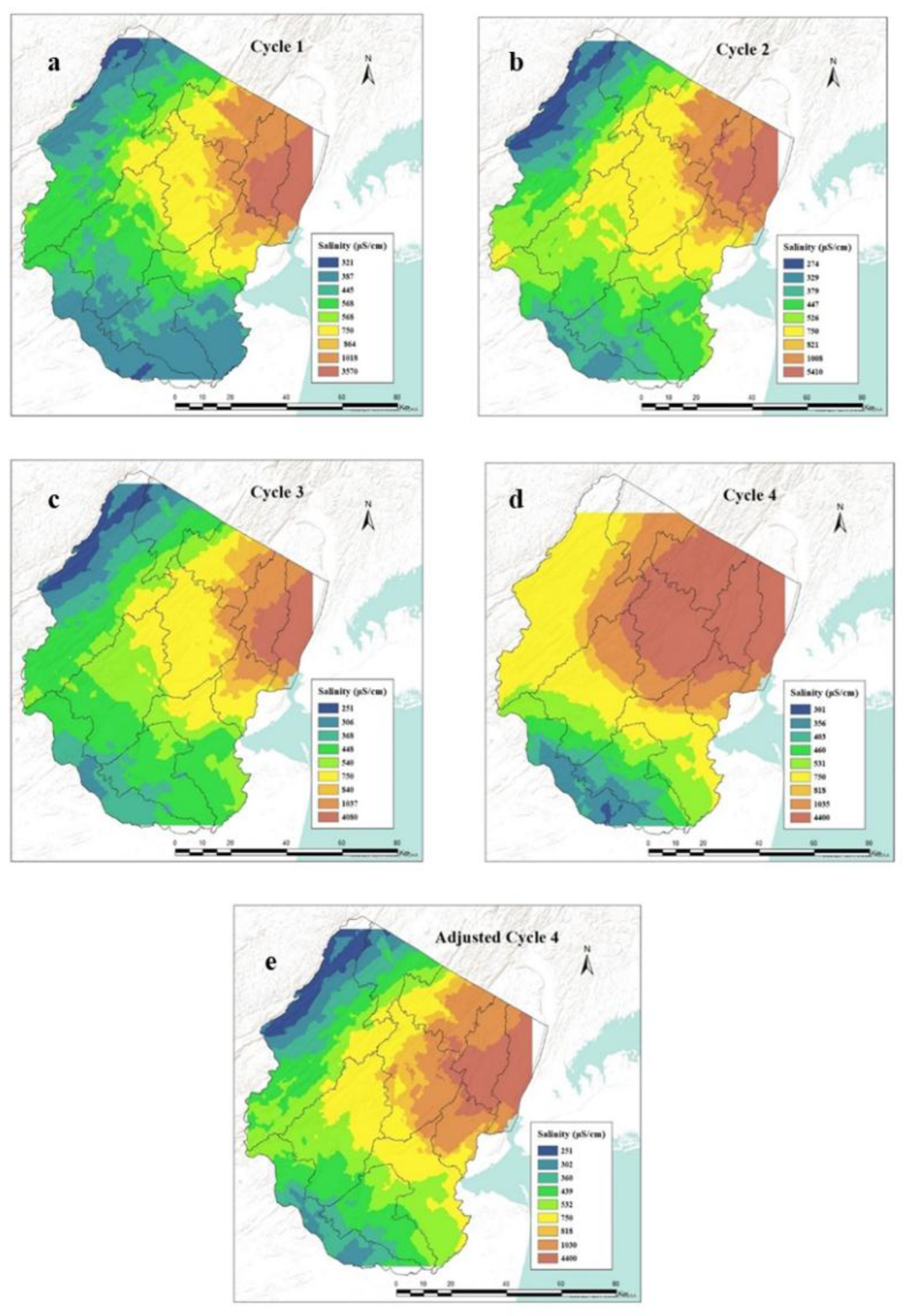
The kriged prediction in sampling cycle 4 (Figure 9d) is unique, showing a concentration pattern that is different from the earlier three sampling cycles. The only noticeable similarity with the previous sampling cycles is that anthropogenic activities have a major influence on the groundwater quality. The kriged map shows that the Northeast is still the region with the most coverage of poor water quality. The uniqueness of sampling cycle 4 is associated with the number of observation wells monitored during this sampling period. This sampling cycle did not include 12 observation wells (about 15 % of the total observations) that were used in the previous three sampling cycles. Sampling cycle 4 had only 65 observation wells as compared to 77 wells in previous sampling cycles. These 12 wells are located within the undeveloped land use (forested) areas that have been shown to have better water quality compared to the other land uses. Nine of these wells are located in the upper part of the study area and two are in the lower part. The omitted wells from the undeveloped land use area in the region usually have low specific conductance values and some of them may be regarded as outliers. As indicated by Johnston et al. [53], such outliers can highly influence kriging estimation values. The kriged prediction map reveals that the Northwest region which had the best groundwater quality coverage in the previous sampling cycles, now shows increased salinity, although most of the specific conductance values are not beyond the 750 μS/cm threshold for freshwater. The omitted observation wells highly influenced the overall spatial autocorrelation of the study area, and this has a major influence on the kriging prediction. The kriging interpolation is not based entirely on the distance between the observed and the estimated points like in other spatial interpolations, but it is based mostly on the weighted average of all the observed points [53]. The kriged map looks different because of the dissimilarity between the measured points and the overall spatial arrangement in the previous sampling cycles. It is known that additional data enhances the performance of kriging predictions. The kriged maps of sampling cycles 1, 2, and 3, showed minimal changes of salinity in the ‘undeveloped (forested) land use’ areas over time. Assuming that this minimal change in salinity will continue into the 4th cycle, it was decided in this study to incorporate the ‘undeveloped land use’ well data from sampling cycle 3 into the sampling cycle 4. This modified sampling cycle is referred to as the ‘Adjusted sampling cycle 4’.
The kriged map from the ‘Adjusted sampling cycle 4’(Figure 9e) shows that spatial distribution of groundwater quality across northern New Jersey is highly related to land use and rapid urbanization. The analysis indicates a general rise in groundwater salinity in the Northeast and Raritan water regions, while the northwest region experienced a decline in salinity. Notably, the Raritan water region displayed a notable increase in salinity for the first time in the adjusted cycle 4. Similarly, the Northeast water region saw some increase in groundwater salinity, making it the water region with the poorest water quality during all the sampling periods.
This study quantifies the coverage of freshwater across the WMAs in northern New Jersey. All the WMAs in northern New Jersey have about 3,400 square miles coverage representing the total coverage of groundwater in the study area. Quantifying the extent of the freshwater coverage in the region enhances the understanding of available freshwater resources, offering insights that go beyond the visual interpretation of the kriged maps. To determine the coverage of freshwater from the kriged map, the raster surfaces were converted to polygons using ArcGIS geostatistical analytical tool and the area of polygons with 750 μS/cm and lesser were calculated to determine the area of freshwater in the study area. During sampling cycle 1 (1999 – 2004), about 80 % of the total coverage of the study area was freshwater. Non-freshwater coverage was observed in sections of WMA – 03 (Pompton), WMA – 04 (lower Passaic), WMA – 05 (Hackensack), WMA – 06 (upper Passaic), and WMA – 07 (Authur Kills). Among these, WMA-04 (Lower Passaic) and WMA-05 (Hackensack) exhibited the highest levels of salinity impact, marking them as the most affected WMAs. Sampling cycle 2 (2004 – 2008) had more coverage of freshwater, about 82.5 % of the total coverage of the study area was freshwater. This is an increase of about 2.5% coverage of freshwater in the study area. Similar to sampling cycle 1, in cycle 2, non-freshwater coverage was also observed in parts of WMA – 03 (Pompton), WMA – 04 (lower Passaic), WMA – 05 (Hackensack), WMA – 06 (upper Passaic), and WMA – 07 (Arthur Kills), with poorer groundwater quality observed in WMA – 04 (lower Passaic) and WMA – 05 (Hackensack). Sampling cycle 3 (2009 – 2013) has similar freshwater coverage as cycle 2, with about 82.4 % of the total coverage of the study area indicating freshwater. Non-freshwater coverage was observed in WMA – 03 (Pompton), WMA – 04 (lower Passaic), WMA – 05 (Hackensack), WMA – 06 (upper Passaic), and WMA – 07 (Arthur Kills), with the poorest groundwater quality observed in WMA – 04 (lower Passaic) and WMA – 05 (Hackensack). WMA – 03 (Pompton) had more freshwater coverage during sampling cycle 3, while there was a decrease in freshwater coverage in Arthur Kills WMA in the same sampling cycle. Sampling cycle 4 (2014 – 2016), which has sparse distribution and influenced by the data’s spatial autocorrelation indicated that about 51% of the total coverage of the study area had freshwater. This is about 30% less freshwater coverage compared to sampling cycle 3. Though statistics of the sampling cycle 4 indicated the highest ‘minimal, maximum and average” value of specific conductance, the spatial prediction of the data was heavily influenced by unavailability of important undeveloped land use data. This concern brought about the ‘adjusted sampling cycle 4’ which includes undeveloped land use data from cycle 3. For the ‘adjusted sampling cycle 4’, the freshwater coverage was about 74%, resulting in a decrease of about 8% in the groundwater quality when compared to sampling cycle 3. Non-freshwater coverages were observed in parts of WMA – 03 (Pompton), WMA – 04 (lower Passaic), WMA – 05 (Hackensack), WMA – 06 (upper Passaic), WMA – 07 (Arthur Kills), WMA – 08 (north Branch Raritan), and WMA – 10 (Millstone), with poorer groundwater quality observed in WMA – 04 (lower Passaic) and WMA – 05 (Hackensack) while WMA – 08, and WMA – 10, indicated a generalized increase in salinity. The kriging interpolation reveals a disturbing trend after four sampling cycles: a steady decline in freshwater coverage. The Northeast water region particularly WMA – 04 (lower Passaic) and WMA – 05 (Hackensack) experienced the most significant impact of freshwater depletion.
4. Conclusions
Kriging interpolation technique proves effective and invaluable for groundwater resources management. This study employed kriging interpolation to spatially analyze groundwater in WMAs across northern New Jersey. Kriging effectively modeled salinity distribution by developing models for the prediction of specific conductance values in locations lacking direct observation. Kriging also facilitated the identification of fresh groundwater coverage in the study area. The spatial and temporal distribution of groundwater quality was assessed.
The findings provide critical insights into freshwater availability and groundwater quality trends over four sampling cycles (1999–2016). Using kriging and GIS tools, the study quantified freshwater distribution, revealing that the Northeast water region had significantly less freshwater coverage compared to the Northwest and Raritan regions. Specific problem areas, such as WMA-04 (Lower Passaic) and WMA-05 (Hackensack) in the Northeast region, consistently exhibited poor groundwater quality due to high salinity, highlighting the need for good water management practices in the area.
The study reveals that anthropogenic activities have had a significant impact on groundwater quality, particularly in the Northeast water region. The spatial analysis identified strong influences of road network density and land use activities on the groundwater quality. The rapid change in land use towards urbanization and the application of deicing salts on the large surface area of the road network appears to be a major control of the deteriorating groundwater quality.
This spatial investigation of groundwater quality in northern New Jersey provides a great insight into groundwater quality in the region. It serves as a beneficial guide to decision-makers and stakeholders, highlighting the need for effective water management strategies in the region. This study is a prelude to more research in the study area. A regionalized and localized study is needed to provide a better understanding of the poor groundwater quality revealed in parts of the northeast water region. It is pertinent to know whether the groundwater contamination is entirely localized or regional. A comprehensive groundwater transport study could indicate if salinity contributions in the Northeast water region originate from activities from surrounding watersheds. It will also be important to know whether the rivers (surface-water bodies) around the watershed are saline, and whether they are losing water into and contaminating the surrounding groundwater.
Author Contributions
Conceptualization, T.O.; methodology, T.O.; software, T.O. and D.O.; validation, T.O.; formal analysis, T.O.; writing—original draft preparation, T.O.; data curation, T.O.; writing—review and editing, T.O. and D.O.; supervision, T.O. and D.O.
Funding
This research was funded by New Jersey Water Resources Research Institute (NJWRRI), grant number, G21AP10595-02.
Data Availability Statement
All data are publicly available and can be accessed at http://wdr.water.usgs.gov.
Conflicts of Interest
The authors declare no conflicts of interest. The funders had no role in the design of the study; in the collection, analyses, or interpretation of data; in the writing of the manuscript; or in the decision to publish the results.
References
- Dieter, C. A., Maupin, M. A., Caldwell, R. R., Harris, M. A., Ivahnenko, T. I., Lovelace, J. K., Barber, N. L., & Linsey, K. S., Estimated use of water in the United States in 2015, U.S. Geological Survey Circular 2018, 1441, 65. [CrossRef]
- Khan, M., Almazah, M. M. A., EIlahi, A., Niaz, R., Al-Rezami, A. Y., and Zaman, B., Spatial interpolation of water quality index based on Ordinary kriging and Universal kriging, Geomatics, Natural Hazards and Risk 2023, 14, 1. [CrossRef]
- Maupin, M. A., Kenny, J. F., Hutson, S. S., Lovelace, J. K., Barber, N. L., and Linsey, K. S., Estimated use of water in the United States in 2010, U.S. Geological Survey Circular 2014, 1405, 56. [CrossRef]
- Reilly, T. E., Dennehy, K. F., Alley, W. M., and Cunningham, W. L., Ground-Water Availability in the United States, U.S. Geological Survey Circular 2008, 1323, 70 Available: https://pubs.usgs.gov/circ/1323/pdf/Circular1323_book_508.pdf.
- Kaushal, S. S., Likens, G. E., Pace, M. L., Reimer, J. E., Maas, C. M., Galella, J. G. … Woglo, S. A. Freshwater salinization syndrome: from emerging global problem to managing risks,” Biogeochemistry 2021 154:2, 255–292, Apr. 2021. [CrossRef]
- Sathe, S. S., and Mahanta, C., Groundwater flow and arsenic contamination transport modeling for a multi aquifer terrain: Assessment and mitigation strategies, J Environ Manage 2019, 231, 166–181. [CrossRef]
- Serfes, M., Bousenberry, R., and Gibs, J., New Jersey Ambient Ground Water Quality Monitoring Network: Status of shallow ground-water quality, 1999-2004, Geological Survey Information Circular 2007. Available: https://www.nrc.gov/docs/ML1408/ML14086A280.pdf.
- Lindsey, B. D., Fleming, B. J., Goodling, P. J., and Dondero, A. M., Thirty years of regional groundwater-quality trend studies in the United States: Major findings and lessons learned, J Hydrol (Amst) 2023, 627, 130427. [CrossRef]
- U.S. Geological Survey, Groundwater Quality, U.S. Geological Survey Water Science School, 2025. Available: https://www.usgs.gov/special-topics/water-science-school/science/groundwater-quality.
- Kaushal, S. S., Groffman, P. M., Likens, G. E., Belt, K. T., Stack, W. P., Kelly V. R. … Fisher, G. T., Increased salinization of fresh water in the northeastern United States, Proceedings of the National Academy of Sciences 2005, 102, 38, 13517–13520. [CrossRef]
- Novotny, E. V., Sander, A. R., Mohseni, O., and Stefan, H. G., Chloride ion transport and mass balance in a metropolitan area using road salt, Water Resour Res 2009, 45, 12. [CrossRef]
- Ophori, D., Firor, C., and Soriano, P., Impact of road deicing salts on the Upper Passaic River Basin, New Jersey: a geochemical analysis of the major ions in groundwater, Environ Earth Sci 2019, 78, 16, 1–13.
- Novotny, V., Muehring, D., Zitomer, D. H., Smith, D. W., and Facey, R., Cyanide and metal pollution by urban snowmelt: impact of deicing compounds, Water Science and Technology 1998, 38, 10, 223–230. [CrossRef]
- Sarkar, D., Preliminary studies on mercury solubility in the presence of iron oxide phases using static headspace analysis, Environmental Geosciences 2003, 10, 4, 151–155, Dec. [CrossRef]
- Bolen W, P., Mineral Commodity Summaries, U.S. Geological Survey 2020.
- New Jersey Department of Transportation (NJDOT), Winter Readiness, Expenditures, About NJDOT, NJDOT 2018, Available: https://www.nj.gov/transportation/about/winter/expenditures.shtm.
- NJDOT, New Jersey’s Roadway Mileage and Daily VMT by Functional Classification Distributed by County, NJDOT 2020, Available: https://www.nj.gov/transportation/refdata/roadway/pdf/hpms2019/VMTFCC_19.pdf.
- Harwell, M. C., Surratt, D. D., Barone, D. M., and Aumen, N. G., Conductivity as a tracer of agricultural and urban runoff to delineate water quality impacts in the northern Everglades, Environ Monit Assess 2008, 147, 1–3, 445–462. [CrossRef]
- Hems, J. D., Study and interpretation of the chemical characteristics of natural water, 3rd ed. U.S. Geological Survey Water-Supply Paper, 1985. Available: https://pubs.usgs.gov/wsp/wsp2254/pdf/wsp2254a.pdf.
- McCleskey, R. B., New method for electrical conductivity temperature compensation, Environ Sci Technol 2013, 47, 17, 9874–9881.
- U.S. Geological Survey, Specific conductance: U.S. Geological Survey Techniques and Methods, book 9, chap. A6.3, 2019. [CrossRef]
- Cartwright, I., Gilfedder, B., and Hofmann, H., Contrasts between estimates of baseflow help discern multiple sources of water contributing to rivers, Hydrol Earth Syst Sci 2014, 18, 1, 15–30, Jan. [CrossRef]
- Clean Water Team (CWT), Electrical conductivity/salinity Fact Sheet, FS-3.1.3.0(EC). in: The Clean Water Team Guidance Compendium for Watershed Monitoring and Assessment, California State Water Resources Control Board 2004.
- Balachandar, D., Sundararaj, P., Murthy, K., and Kumaraswamy, K., An Investigation of Groundwater Quality and Its Suitability to Irrigated Agriculture in Coimbatore District, Tamil Nadu, India - A GIS Approach, International Journal on Environmental Sciences 2010, 1, 176-190.
- US EPA, 5.9 Conductivity | Monitoring & Assessment. US EPA 2012, Available: https://archive.epa.gov/water/archive/web/html/vms59.html.
- United States Salinity Laboratory Staff (USSL), Diagnosis and Improvement of Saline and Alkaline Soils, Soil Science Society of America Journal 1954, 18, 3, 348–348. [CrossRef]
- Raritan Basin Watershed Management Project, Raritan Basin: Portrait of a Watershed. New Jersey Water Supply Authority – Watershed Protection Programs, 2002. Available: https://rucore.libraries.rutgers.edu/rutgers-lib/17036/.
- Lathrop, R. G., Measuring Land Use Change in New Jersey: Land Use Update to Year 2000, A Report on Recent Development Patterns 1995 to 2000, Grant F. Walton Center for Remote Sensing & Spatial Analysis (CRSSA) 2004, 17-2004-1. Available: https://crssa.rutgers.edu/projects/lc/docs/landuse_upd.pdf.
- Arslan, H., Spatial and temporal mapping of groundwater salinity using ordinary kriging and indicator kriging: The case of Bafra Plain, Turkey, Agric Water Manag 2012, 113, 57–63. [CrossRef]
- Belkhiri, L., Tiri, A., and Mouni, L., Spatial distribution of the groundwater quality using kriging and Co-kriging interpolations, Groundw Sustain Dev 2020, 11, 100473. [CrossRef]
- Elubid, B. A., Ahmed, E. H., Zhao, J., Elhag, K. M., Abbass, W., and Babiker, M. M., Geospatial Distributions of Groundwater Quality in Gedaref State Using Geographic Information System (GIS) and Drinking Water Quality Index (DWQI), Int J Environ Res Public Health 2019, 16, 5, 731. [CrossRef]
- Gharbia, A. S., Gharbia, S. S., Abushbak, T., Wafi, H., Aish, A., Zelenakova, M. & Pilla, F., Groundwater Quality Evaluation Using GIS Based Geostatistical Algorithms, Journal of Geoscience and Environment Protection 2016, 04, 02, 89–103. [CrossRef]
- Johnson, C. D., Nandi, A., Joyner, T. A., and Luffman, I., Iron and Manganese in Groundwater: Using Kriging and GIS to Locate High Concentrations in Buncombe County, North Carolina, Groundwater 2018, 56, 1, 87–95. [CrossRef]
- Li, J., Heap, A. D., Potter, A., Huang, Z., and Daniell, J. J., Can we improve the spatial predictions of seabed sediments? A case study of spatial interpolation of mud content across the southwest Australian margin, Cont Shelf Res 2011, 31, 13, 1365–1376. [CrossRef]
- Jalan, S., Chouhan, D. S., and Chaure, S., Geospatial Analysis of Spatial Variability of Groundwater Quality Using Ordinary Kriging: A Case Study of Dungarpur Tehsil, Rajasthan, India, Journal of Geomatics 2022, 16, 2, 176–187. [CrossRef]
- Van Beers, W. C. M., and Kleijnen, J. P. C., Kriging Interpolation in Simulation: A Survey, in Proceedings of the 2004 Winter Simulation Conference, R. G. Ingalls, M. D. Rossetti, J. S. Smith, and B. A. Peters, Eds., 2004. Available: https://informs-sim.org/wsc04papers/014.pdf.
- Tyagi, A., and Singh, P., Applying Kriging Approach on Pollution Data Using GIS Software, International Journal of Environmental Engineering and Management 2013, 4, 3, 185–190, Available: http://www.ripublication.com/ijeem.htm.
- Siska, P. P., and Hung, I., Assessment of Kriging Accuracy in the GIS Environment, in The 21st Annual ESRI International User Conference, San Diego, CA, 2001, Available: https://proceedings.esri.com/library/userconf/proc01/professional/papers/pap280/p280.htm.
- Royle, J. A., and Nichols, J. D., Estimating Abundance from Repeated Presence-Absence Data or Point Counts - Tulane University, Ecology 2003, 84, 3, 777–790, Available: https://library.search.tulane.edu/discovery/fulldisplay?docid=cdi_proquest_miscellaneous_18770213&context=PC&vid=01TUL_INST:Tulane&lang=en&search_scope=MyInst_and_CI&adaptor=Primo%20Central&query=null,,PDF,AND&facet=citing,exact,cdi_FETCH-LOGICAL-c2640-4cc3ab70d55b63c5a41a56af47e37e4d20dae7847301f73cc0489de23a2d78ec3&offset=2.
- New Jersey Department of Environmental Protection, New Jersey’s Watersheds, Watershed management Areas and Water Regions, NJDEP Division of Watershed Management 1997. Available: https://dep.nj.gov/earthday/timeline/m1997/.
- Watt, M. K., A Hydrologic Primer for New Jersey Watershed Management, USGS Water-Resources Investigations Report, West Trenton, New Jersey, 2000. Available: https://pubs.usgs.gov/wri/2000/4140/report.pdf.
- Dalton, R. F., Monteverde, D. H., Sugarman, P. J., and Volkert, R. A., Bedrock Geologic map of New Jersey, New Jersey Geological Survey 2014. Available: https://www.nj.gov/dep/njgs/pricelst/Bedrock250.pdf.
- Drake, A. A., Jr., Volkert, R. A., Monteverde, D. H., Herman, G. C., Houghton, H. F., Parker, R. A., & Dalton, R. F., Bedrock geologic map of northern New Jersey, U. S. Geological Survey 1997. [CrossRef]
- New Jersey Department of Environmental Protection, Bedrock Geologic Map of New Jersey and Bedrock Geology of New Jersey, NJDEP – New Jersey Geological and Water Survey - U. S. Geological Survey 2016. Available: https://www.nj.gov/dep/njgs/enviroed/freedwn/psnjmap.pdf.
- Dalton, R., Physiographic Provinces of New Jersey, New Jersey Geological Survey Informational Circular 2003. Available: https://www.nj.gov/dep/njgs/enviroed/infocirc/provinces.pdf.
- Bousenberry, R., New Jersey Ambient Ground Water Quality Monitoring Network: New Jersey Shallow Ground-Water Quality, 1999 – 2008, New Jersey Geological and Water Survey Information Circular 2016. Available: https://www.nj.gov/dep/njgs/enviroed/infocirc/NJAGWQMN.pdf.
- R – Core Team, R: A Language and Environment for Statistical Computing, R Foundation for Statistical Computing, Vienna, Austria 2023.
- QGIS.org, QGIS Geographic Information System. Open-Source Geospatial Foundation Project, n.d. Available: https://qgis.org/.
- ESRI, ArcGIS Pro: Understanding how to remove trends from the data, ESRI – ArcGIS n.d. Available: https://pro.arcgis.com/en/pro-app/latest/help/analysis/geostatistical-analyst/understanding-how-to-remove-trends-from-the-data.htm.
- Almodaresi, S. A., Mohammadrezaei, M., and Dolatabadi, M., Qualitative Analysis of Groundwater Quality Indicators Based on Schuler and Wilcox Diagrams: IDW and Kriging Models, J Environ Health Sustain Dev 2019, 4, 4, 903–915. [CrossRef]
- Boudibi, S., Sakaa, B., and Zapata-Sierra, A. J., Groundwater Quality Assessment Using GIS, Ordinary Kriging and WQI in an Arid Area, PONTE International Scientific Researchs Journal 2019, 75, 12. [CrossRef]
- Hengl, Tomislav, A Practical Guide to Geostatistical Mapping of Environmental Variables. Office for Official Publications of the European Communities; JRC38153, 2007. Available: https://publications.jrc.ec.europa.eu/repository/handle/JRC38153.
- Johnston, K., Ver Hoef, J. M., Krivoruchko, K., and Lucas, N., Using ArcGIS geostatistical analyst: GIS by ESRI, Redlands, California: Esri Press, 2001.
- Krivoruchko, K., Spatial statistical data analysis for GIS users, 1st ed. Redlands, California: Esri Press, 2011.
- Bajjali, W., ArcGIS for Environmental and Water Issues, Springer Textbooks in Earth Sciences, Geography and Environment 2018. [CrossRef]
- Chiu, S. N., Spatial Point Pattern Analysis by using Voronoi Diagrams and Delaunay Tessellations – A Comparative Study, Biometrical Journal 2003, 45, 3, 367–376. [CrossRef]
- Nayanaka, V., Vitharana, W., and Mapa, R., Geostatistical Analysis of Soil Properties to Support Spatial Sampling in a Paddy Growing Alfisol, Tropical Agricultural Research 2011, 22, 1, 34. [CrossRef]
- Thomas, E. O., Spatial evaluation of groundwater quality using factor analysis and geostatistical Kriging algorithm: a case study of Ibadan Metropolis, Nigeria, Water Pract Technol 2023, 18, 3, 592–607. [CrossRef]
- Al-Omran, A. M., Aly, A. A., Al-Wabel, M. I., Al-Shayaa, M. S., Sallam, A. S., and Nadeem, M. E., Geostatistical methods in evaluating spatial variability of groundwater quality in Al-Kharj Region, Saudi Arabia, Appl Water Sci 2017, 7, 7, 4013–4023. [CrossRef]
- Trangmar, B. B., Yost, R. S., and Uehara, G., Application of Geostatistics to Spatial Studies of Soil Properties, Advances in Agronomy 1985, 38, 45–94. [CrossRef]
- Lloyd, C. D., Local models for spatial analysis, 2nd ed. CRC Press, 2010.
- Jarmołowski, W., Wielgosz, P., Ren, X., and Krypiak-Gregorczyk, A., On the drawback of local detrending in universal kriging in conditions of heterogeneously spaced regional TEC data, low-order trends and outlier occurrences, J Geod 2021, 95, 1, 2. [CrossRef]
- Rossi, M. L., Kremer, P., Cravotta, C. A., Seng, K. E., and Goldsmith, S. T., Land development and road salt usage drive long-term changes in major-ion chemistry of streamwater in six exurban and suburban watersheds, southeastern Pennsylvania, 1999–2019, Front Environ Sci 2023, 11. [CrossRef]
- Marghade, D., Malpe, D. B., and Subba Rao, N., Identification of controlling processes of groundwater quality in a developing urban area using principal component analysis, Environ Earth Sci 2015, 74, 7, 5919–5933. [CrossRef]
- Sun, H., Huffine, M., Husch, J., and Sinpatanasakul, L., Na/Cl molar ratio changes during a salting cycle and its application to the estimation of sodium retention in salted watersheds, J Contam Hydrol 2012, 136–137, 96–105. [CrossRef]
Figure 1.
Map of northern New Jersey (a) water regions and WMAs, and (b) Land use, adapted from Watt [41].
Figure 1.
Map of northern New Jersey (a) water regions and WMAs, and (b) Land use, adapted from Watt [41].
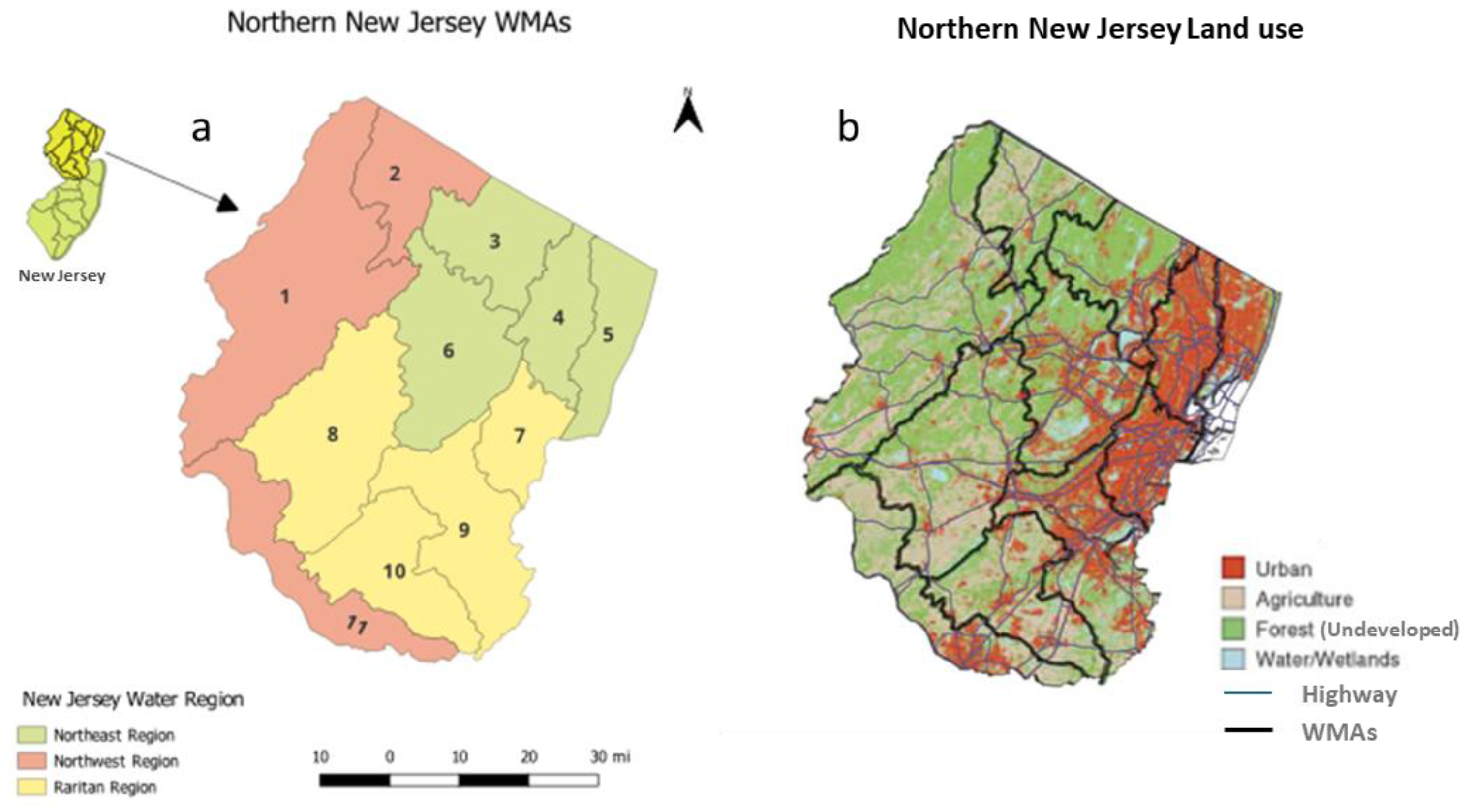
Figure 2.
Flowchart of spatial analysis (kriging interpolation).
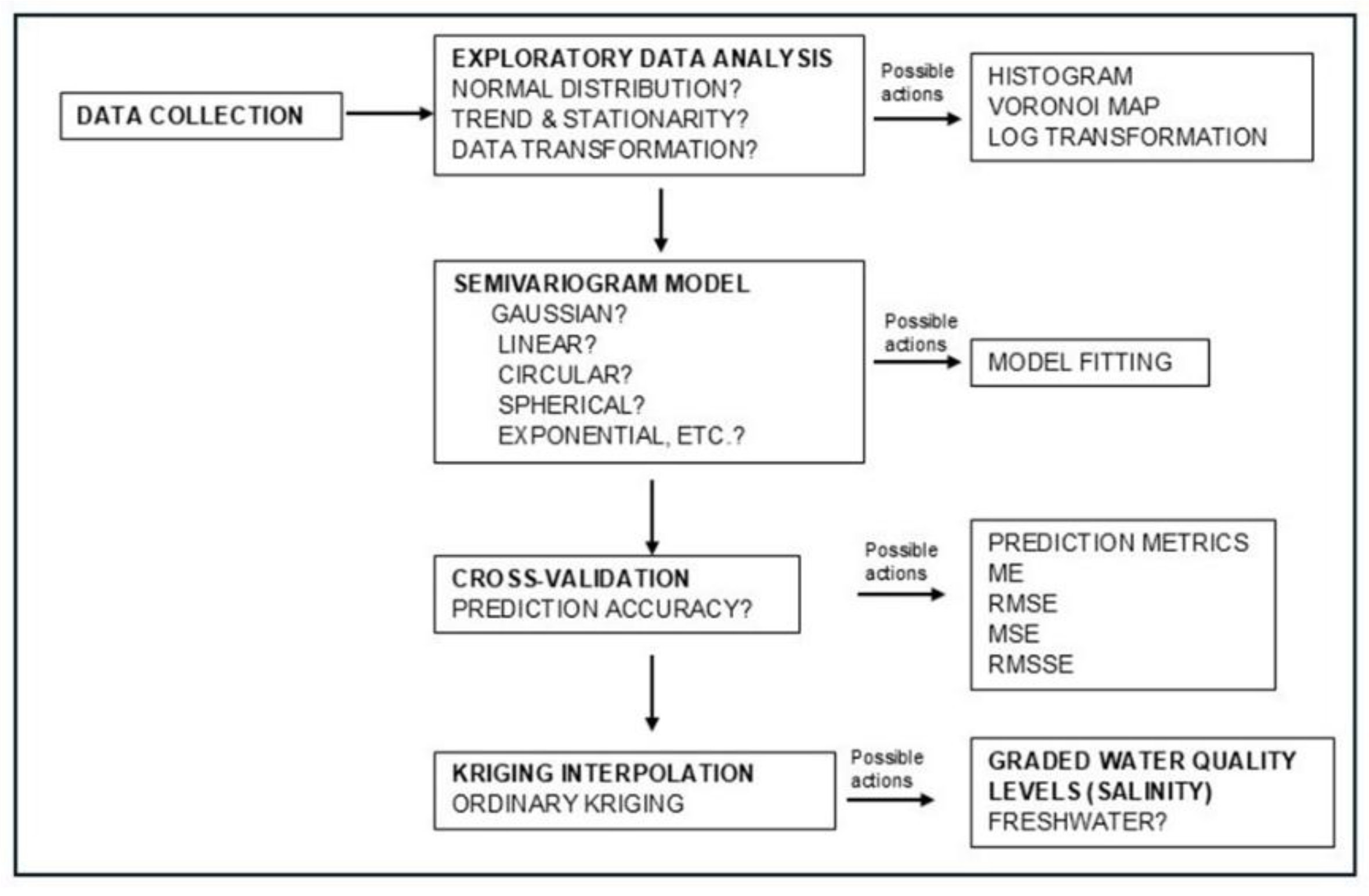
Figure 3.
Semivariogram graph (adapted from Jalan et al. [35]).
Figure 3.
Semivariogram graph (adapted from Jalan et al. [35]).
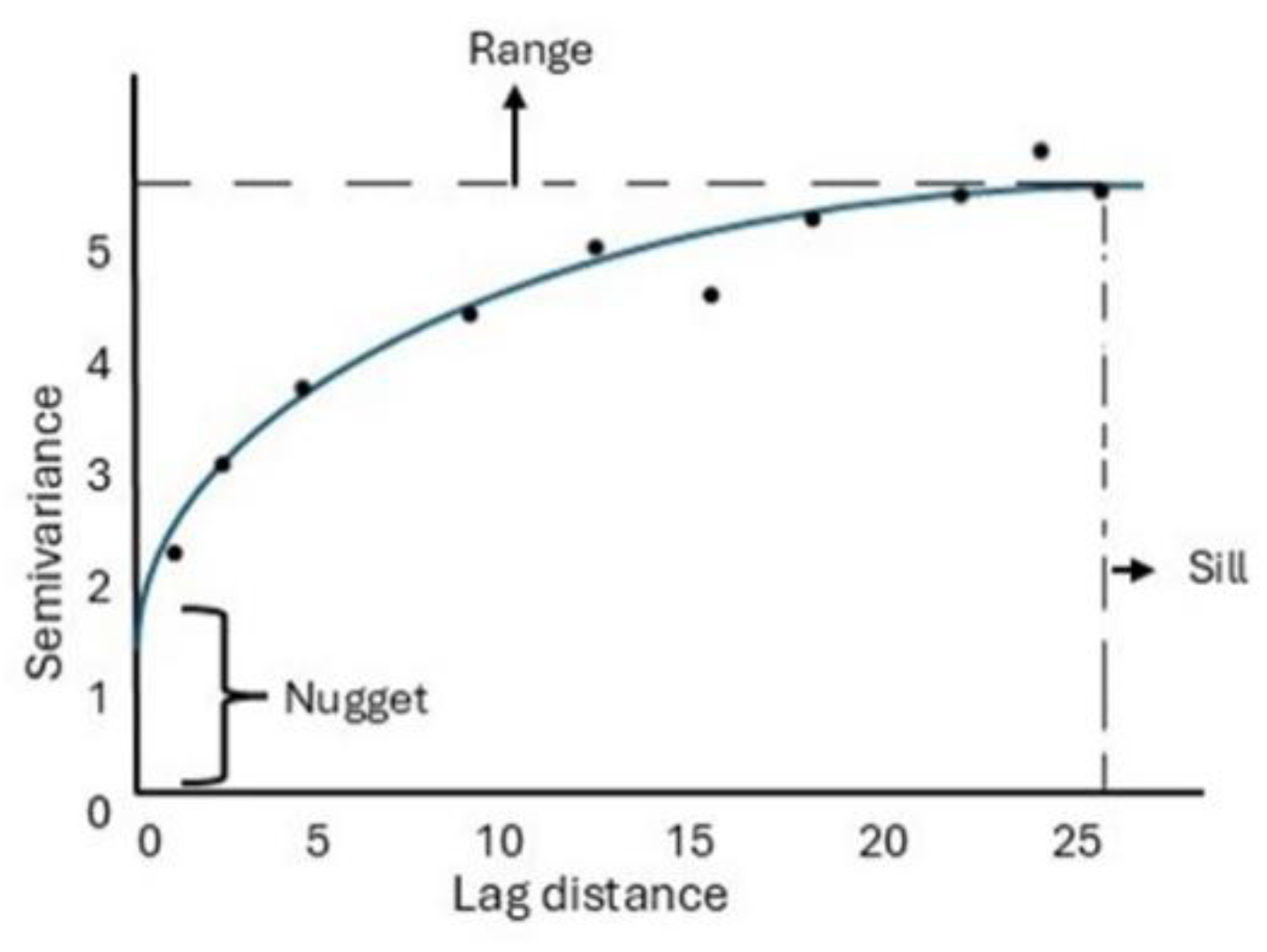
Figure 4.
Histogram of the data for all sampling cycles.
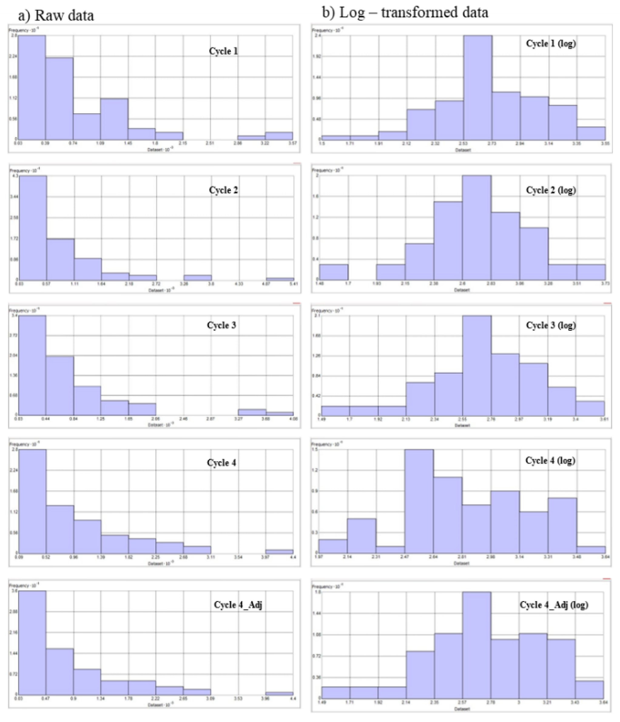
Figure 5.
Q-Q Plots of data for all Sampling cycles.
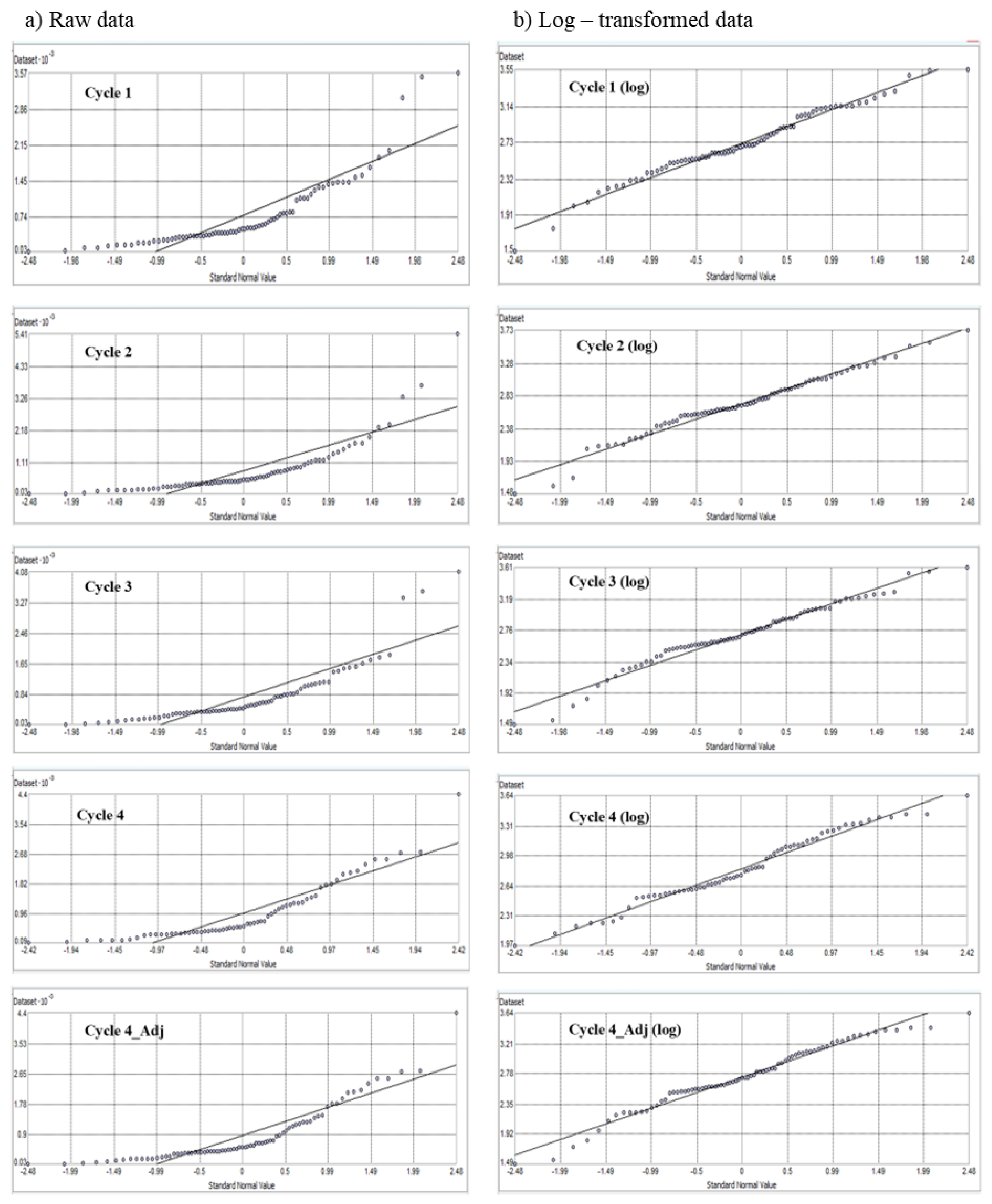
Figure 6.
Voronoi map of data for all Sampling cycles (including an Illustration of trend).
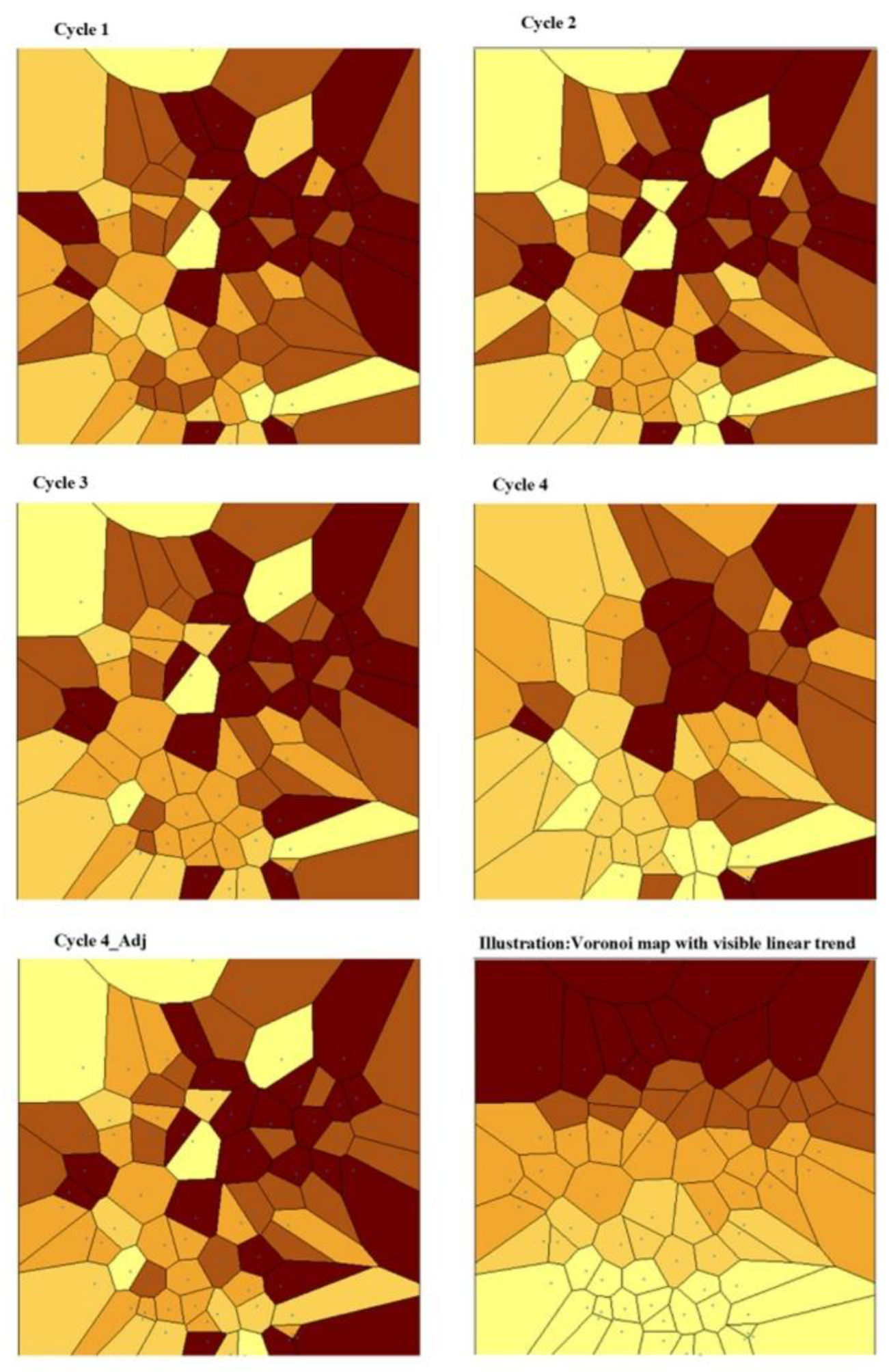
Figure 7.
Plotted Semivariograms for all Sampling cycles.
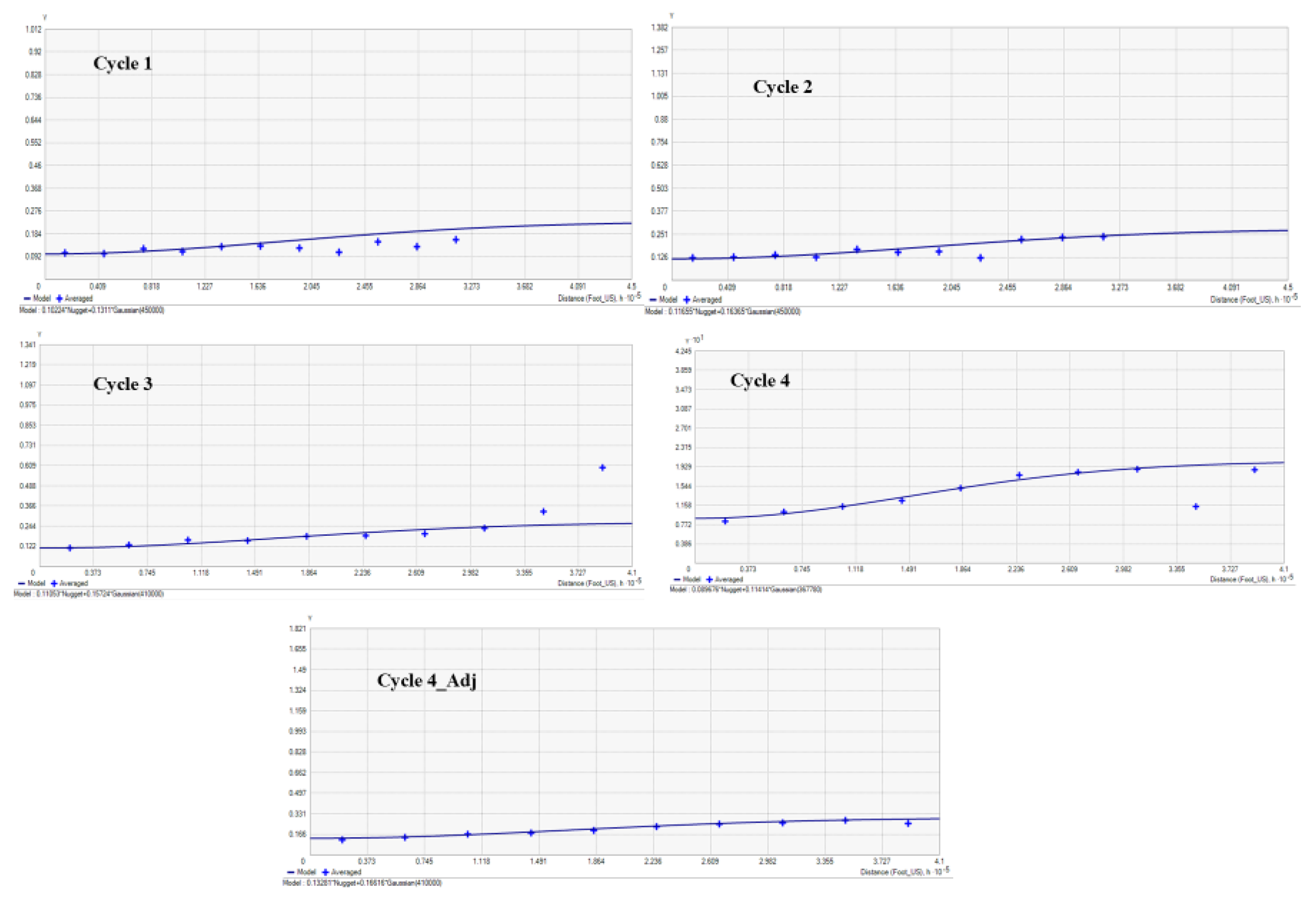
Figure 8.
Salinity map overlaid with (a) Highway (b) All major roads.
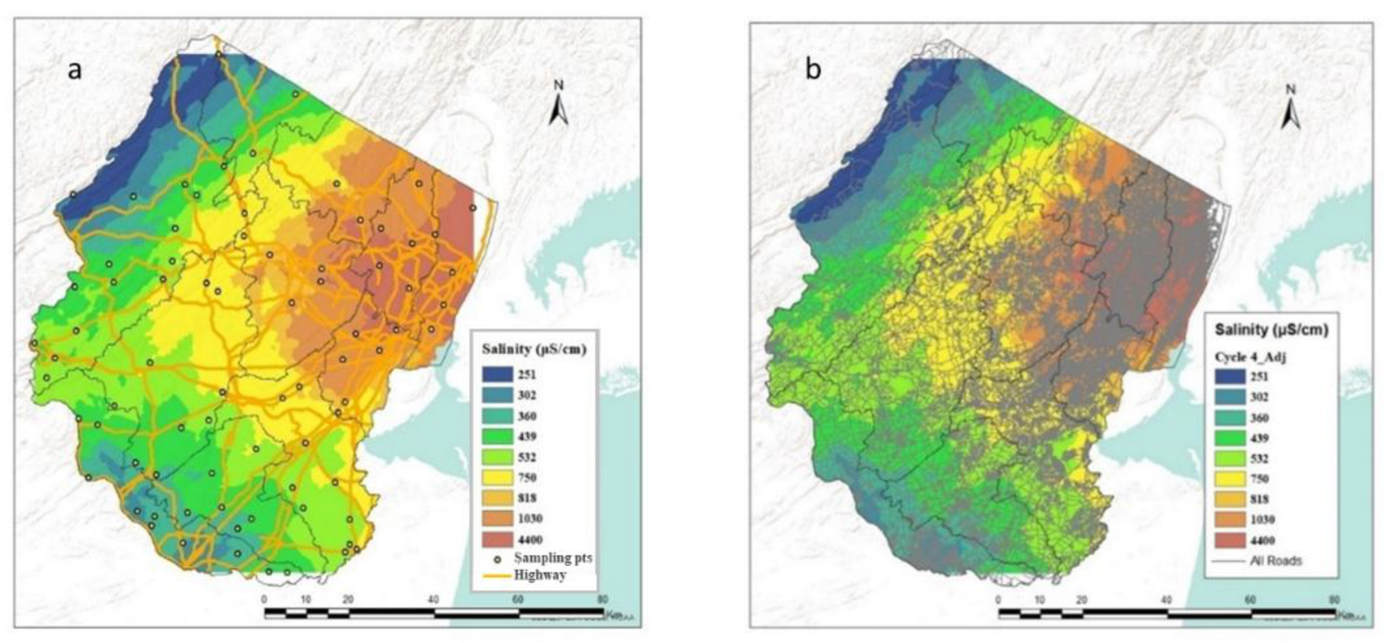

Table 1.
Statistics summary for Specific Conductance.
| Sampling cycles | SC | Log SC | |
|---|---|---|---|
| Cycle 1 | mean | 755.28 | 2.718 |
| n =76 | median | 485 | 2.686 |
| skewness | 2.1455 | -0.2679 | |
| kurtosis | 8.1825 | 3.039 | |
| Cycle 2 | mean | 799.03 | 2.717 |
| n =77 | median | 494 | 2.694 |
| skewness | 2.9129 | -0.362 | |
| kurtosis | 13.645 | 3.773 | |
| Cycle 3 | mean | 759.53 | 2.7043 |
| n =76 | median | 487 | 2.687 |
| skewness | 2.4312 | -0.50483 | |
| kurtosis | 9.8845 | 3.7461 | |
| Cycle 4 | mean | 955.66 | 2.8261 |
| n =65 | median | 577 | 2.761 |
| skewness | 1.616 | 0.00639 | |
| kurtosis | 5.9171 | 2.3403 | |
| Cycle 4Adj | mean | 848.27 | 2.7319 |
| n =77 | median | 527 | 2.7218 |
| skewness | 1.756 | -0.44241 | |
| kurtosis | 6.5282 | 3.1793 |
Note. SC – Specific Conductance values, n = number of samples, Adj – Adjusted.
Table 2.
Semivariogram model performance metrics.
| Sampling cycles | MSE | RMSSE | RMSE | ASE |
|---|---|---|---|---|
| Cycle 1 | - 0.0096 | 1.0899 | 0.3706 | 0.3347 |
| Cycle 2 | - 0.01329 | 1.1382 | 0.4148 | 0.3576 |
| Cycle 3 | - 0.00997 | 1.1478 | 0.4095 | 0.3496 |
| Cycle 4 | - 0.01506 | 1.0265 | 0.3254 | 0.3165 |
| Cycle 4_Adj | - 0.01296 | 1.1094 | 0.4309 | 0.3824 |
Note. Adj – Adjusted.
Disclaimer/Publisher’s Note: The statements, opinions and data contained in all publications are solely those of the individual author(s) and contributor(s) and not of MDPI and/or the editor(s). MDPI and/or the editor(s) disclaim responsibility for any injury to people or property resulting from any ideas, methods, instructions or products referred to in the content. |
© 2025 by the authors. Licensee MDPI, Basel, Switzerland. This article is an open access article distributed under the terms and conditions of the Creative Commons Attribution (CC BY) license (http://creativecommons.org/licenses/by/4.0/).
Copyright: This open access article is published under a Creative Commons CC BY 4.0 license, which permit the free download, distribution, and reuse, provided that the author and preprint are cited in any reuse.


