Preprint
Article

This version is not peer-reviewed.

Small Defects Detection of Galvanized Strip Steel via Schatten-p Norm-Based Low-Rank Tensor Decomposition

A peer-reviewed article of this preprint also exists.

Submitted:

28 February 2025

Posted:

03 March 2025

You are already at the latest version

Abstract

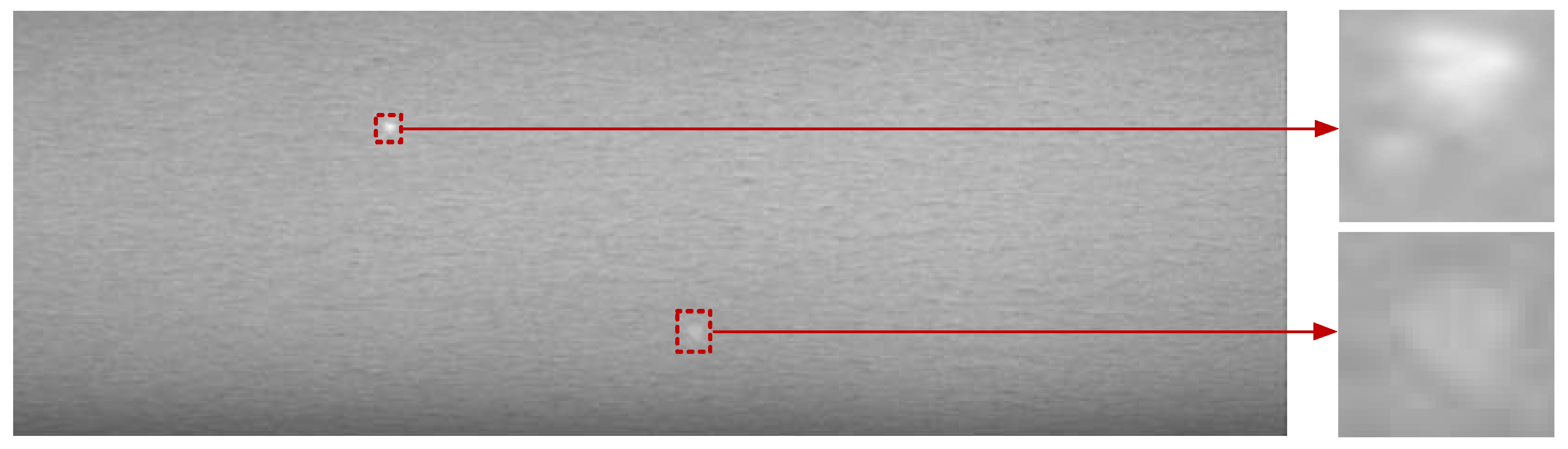
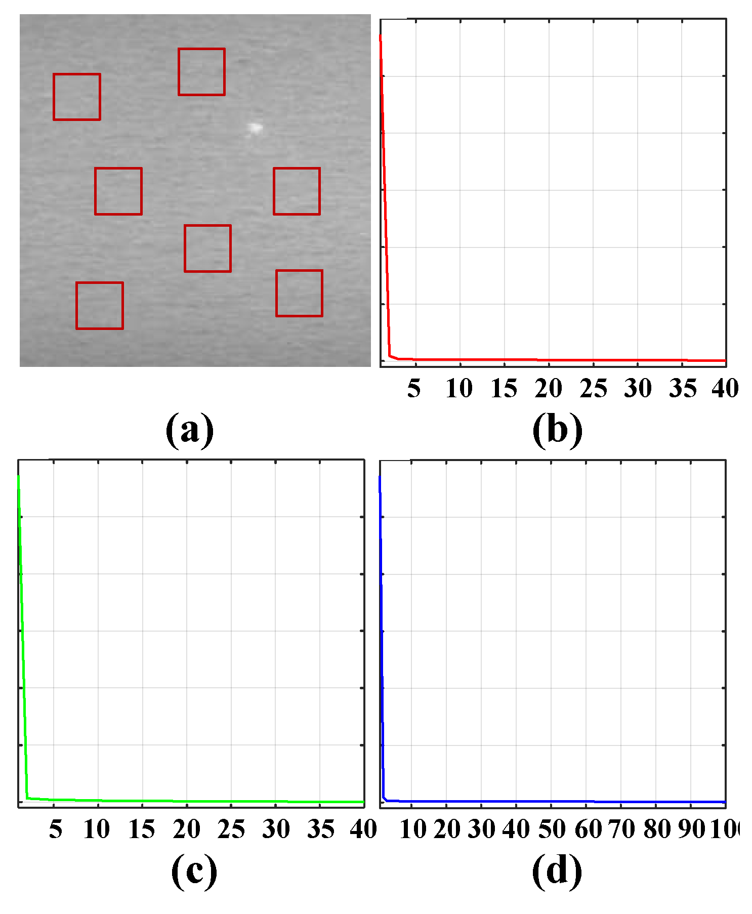
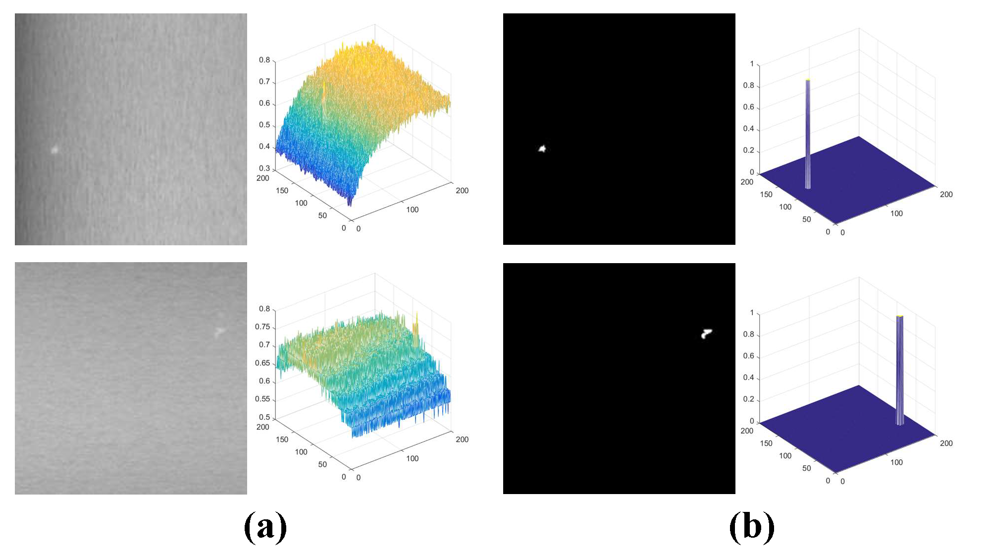
Accurate and efficient white-spot defects detection for the surface of galvanized strip steel is one of the most important guarantees for the quality of steel production. It’s a fundamental but “hard” small target detection problem due to its small pixel occupation in low-contrast images. By fully exploiting the low-rank and sparse prior information of surface defect image, a Schatten-p norm-based low-rank tensor decomposition (SLRTD) method is proposed to decomposes the defect image into low-rank background, sparse defect, and random noise. Firstly, the original defect images are transformed into a new patch-based tensor mode through data reconstruction for mining valuable information of defect image. Then, considering the over-shrinkage problem in low-rank component estimation caused by vanilla nuclear norm and weighted nuclear norm, a nonlinear reweighting strategy based on Schatten p-norm is incorporated to improve the decomposition performance. Finally, a solution framework is proposed via a well-designed alternating direction method of multipliers to obtain the white-spot defect target image by a simple segmenting algorithm. The white-spot defect dataset from real-world galvanized strip steel production line is constructed, and the experimental results demonstrate that the proposed SLRTD method outperforms existing state-of-the-art methods qualitatively and quantitatively.

Keywords: 
;  ;  ;  

1. Introduction

The galvanized strip steel is widely used in automobile manufacturing, household electrical appliances and other daily-use products, surface defects might lead to some product quality issues for both in-progress and downstream products. Among various types of surface defects, white-spot defects that as shown in Figure 1, mainly caused by random zinc dross and ash in the hot dip or electro galvanizing process, are considered as the most serious threat to the steel surface quality due to their high concurrence and typical periodicity. This defect can be detected and recorded by the surface defect inspection based on machine vision, and then the quality issues with strip steel will be controlled at the early stage [1,2].
For galvanized steel sheet, the white-spot defects are always ultra-tiny in size, occupying less than 5% of the whole raw image, the shape and size of each defect are greatly different, and the defect does not have a clear semantic relationship with the complex background. Not only are these objects tiny in size, they also lack feature information of color or texture. In fact, industrial production images frequently contain some prior information, for example, defect rarely appears, the vast majority of images is no defect. The inherent issues of tiny size and low-contrast of white-spot defect under complex clutters and heavy noise. poses a challenge on the localization and segmentation of this defect: (a) they are sensitive to tiny defects because of their extreme small sizes, and (b) they cannot accurately locate the random appeared defects whose semantic relationship with the background context is weak.
In the field of machine vision, small or tiny object detection has always been a hot study issue, especially in industrial applications [3,4,5,6,7]. These researches can be classified into three categories: traditional filtering-based methods, sparse and low-rank representation-based methods, and data-driven methods [8]. Filtering-based methods typically design relevant filtering operators in either grayscale or derivative spaces to suppress background noise and enhance targets. While these methods offer a certain level of real-time performance, they often require manual design of operators tailored to specific scenes when facing complex backgrounds, which limits their generalization ability and adaptability. Unlike the methods above that rely on manually designed features based on data priors, data-driven approaches utilize convolutional neural networks (CNNs) for deep feature extraction automatically [9,10]. Although these methods perform well and can extract deeper information, they depend heavily on image samples, which affects their real-time applicability. Additionally, the cost of obtaining a large amount of labeled datasets is often prohibitively high. Furthermore, most deep learning methods exhibit poor generalization capabilities in test datasets that differ from the training datasets. Moreover, due to the size limitations of small targets, which typically consist of only a few pixels, there is a risk of losing critical information during target detection, which may be ineffective or even degrade detection performance. In contrast, some traditional methods offer strong interpretability and maintain a certain level of robustness when faced with complex scenarios, maintaining certain advantages.
In recent years, tensor decomposition-based sparse and low-rank representation methods have achieved remarkable success, especially in infrared or remote sensing small target detection [11,12,13,14,15]. These methods leverage the low-rank nature of the infrared background and the sparse characteristics of small infrared targets, the background is modeled as a low-rank component, while the infrared targets are typically modeled as sparse components. The tensor model effectively preserves spatial structures and utilizes temporal information across multiple frames, which helps achieve more accurate target detection. These methods can combine spatial and temporal local information and iteratively optimize to approach the optimal detection results, significantly improving robustness to detect small targets in complex scenes. Due to distinct domains and different concerns, the aforementioned methods are less widely applied for defect detection in real-world industrial field, such as surface defect detection for the printed circuit board [16], tiny target detection for steel sheet. They may fail without temporal information across frames.
As the defect is random in the production line of strip steel, different image frames are irrelated, and the spatial and temporal information between different image frame is lost. As single-frame information is limited, these methods often miss targets or retain excessive false alarms when dealing with edge overlapping or complex backgrounds, thus failing to provide optimal decomposition guidance. As shown in Figure 1, the white-spot defect of galvanized steel sheet is random and keeps changing all the time, small or tiny white-spot among 4096×2048 raw images, are still easily ignored due to insufficient appearance information. At the same time, the highly varied nature of the background image and small target characteristics make the detection process extremely difficult.
Motivated by the above discussions, there is a need to develop an advanced object detection framework for tiny defect detection for steel sheet. This article thoroughly takes into account the production intrinsic prior to emphasizes the importance of establishing adaptive tensor model to accurately detect small defects on galvanized steel sheet.
The main contributions of this article are outlined as follows:
  • We propose a SLRTD method by digging out inter-patch correlation-ships of surface defect images of galvanized strip steel. The separated defect foreground target information with sparse outliers is embedded in the background of low-rank representation.
  • To achieve an accurate estimation of non-defect background rank, we incorporate weighted Schatten p-norm regularization for the background component, allowing for better noise removal while preserving edges, ultimately leading to improved detection results. Concurrently, a nonlinear reweighting strategy and tensor singular value decomposition (t-SVD) are adopted to help the model more delicately balance the low-rank and sparse components throughout the iterative process, which elevates the separation accuracy between the defect target and non-defect background.
  • On the basis of the alternating direction method of multipliers (ADMM), an effective approach is introduced to solve the sparse and low-rank component decomposition problem. Experiments validate the feasibility and effectiveness of the proposed SLRTD method.
The remainder of this paper is structured as follows: Section 2 provides a concise overview of related work. Section 3 presents a comprehensive introduction to the architecture and components of the proposed SLRTD approach. Section 4 demonstrates numerical comparisons and module analysis. Finally, Section 5 concludes with a discussion of future research prospects. In our paper, tensors, matrices, and vectors are denoted using calligraphic letters, uppercase, and lowercase italics.

2. Related Works

In this section, we provide a brief overview of existing defect detection methods based on filtering, data-driven and tensor decomposition methods.

2.1. Filtering-Based Methods

Generally, filter-based methods design relevant filtering operators in grayscale or derivative spaces to suppress background clutter and enhance the target. These methods can be further classified into threshold method (e.g., Otsu, cross-entropy), morphological method (e.g., morphological operations, template matching), and spectral method (e.g., Fourier transform, Gabor transform, wavelet transform). However, threshold and morphological methods often have difficulties to determine the optimal threshold and need manual adjustments to find the defect regions, especially when the distributions of scene intensity and texture are complicated. The spectral method transform digital images from time-domain into frequency-domain are not sensitive to small objects in the image, so that often miss some small defects in metal surface inspection. Machine learning methods usually include the two-stage of feature extraction and pattern classification [17]. Man-made features are extracted and used by the classifier to predict the defect types. These features include the local binary pattern features, histogram of oriented gradient features, and some other grayscale statistical features. However, these man-made features are still sensitive to defect shape variances, different lighting conditions and background conditions, lacking generalization ability, and showing poor adaptability and robustness.

2.2. Data-Driven-Based Methods

During the past few years, tremendous efforts have been devoted to small defect target detection based on deep learning [18]. Zhang et al. [19] constructed a novel feature enhancement network to improve the performance of small object detection. Hou et al. [20] proposed a contextual information and spatial attention that is based network for detecting small defects in manufacturing industry. Yang et al. [21] introduced RSADUnet model for metal surface tiny defect inspection. However, the satisfactory performance of these methods relies heavily on expensive labeled images, big numbers of parameters and computational complexity to obtain strong feature awareness. Additionally, they are mainly used for natural scene or objects and medical images detection that the shape of these objects does not change much, but the shapes of the metal surface defects are quite different. Thus, these methods may not suitable for metal surface defect inspection in the industry, especially for small defects with varied shapes. At the same time, small defect targets occupy little pixels and lack obvious texture and structure characteristics. These small defects with fewer pixels coverage are not easy to draw attention and provide reliable features.

2.3. Tensor Decomposition-Based Methods

In contrast, tensor decomposition-based sparse and low-rank model always transform the detection problem into an iterative optimization task by exploring new representations of the target and background features. Each patch is directly used as the obverse side slice to construct tensor data, which can guarantee the local features of defect image can be reserved and is conductive to withdrawing the prior information. Many methods proposed different regularization to constrain low-rank and sparse attributes. The reweighted infrared patch-tensor model (RIPT) model proposed by Dai et al. [22] utilizes the target sparse prior and background nonlocal self-correlation prior, and the local structure weight is designed for the target tensor term and served as an edge indicator in the weighted model. However, RIPT still has limitations because the nuclear norm cannot accurately estimate the background. To alleviate this issue, inspired by t-SVD and non-convex approximation of rank based on the tensor nuclear norm, Lu et al. [23] exploited tensor robust principal component (TRPCA) method, which regularizes all singular values of tensor data equally and shrinks all singular values with the same parameter. Zhang et al. [24] introduced a novel nonconvex low-rank constraint, partial sum of the tensor nuclear norm (PSTNN), combining with a weighted l1 norm to effectively suppress the background while that effectively preventing target over-shrinkage. Gao et al. [25] developed an enhanced TRPCA (ETRPCA) model by the weighted tensor Schatten p-norm minimization, which makes the large singular values shrink less in tensor nuclear norm minimization. The Schatten p-norm can better approximate the NP-Hard problem, optimize the recovery of its convex relaxation and will not over-shrink the low-rank components of the data. Chen et al. [26] introduced logarithmic norm regularization as the nonconvex surrogate of matrix and tensor rank, which achieves more accurate low-rank approximation and high computational efficiency.
As it does not consider the influence from noise and clutter, the target detection effect will be reduced greatly in the face of defect image in more complex background. Luo et al. [27] utilized the sparse components of small targets along with a background dictionary, employing the fully connected tensor nuclear norm for low-rank estimation. Wang et al. [28] built a unique regularization term as tensor correlated total variation, which essentially encodes both low-rank and sparse priors of a tensor simultaneously. Geng et al. [29] developed a nonconvex and nonlocal TRPCA (NN-TRPCA) model based on the tensor adjustable logarithmic norm, which adaptively shrink small singular values more and shrink large singular values less. The weighted parameters are manually set as per different scene demands, and they cannot achieve self-adaptive adjustment to avoid influencing the detection effect. Huang et al. [30] introduced a two-stage feature complementary improved tensor low-rank sparse decomposition method, which is divided into two stages: tensor initialization and tensor decomposition, effectively integrating local and nonlocal features. Based on above analysis, the detection capability of these methods is dependent on the contrast between the target and the background. When there is strong contrast, these methods yield good detection results, otherwise, they tend to have a high false positive rate. Moreover, these methods depend on the measurement of background rank in terms of accuracy, and obviously reduces performance and is time-consuming in the face of dim target with complex background.

3. Methodology

The overall framework of the proposed SLRTD method is shown in Figure 2, which consists of construction of tensor model for defect image, model solution, and model analysis.

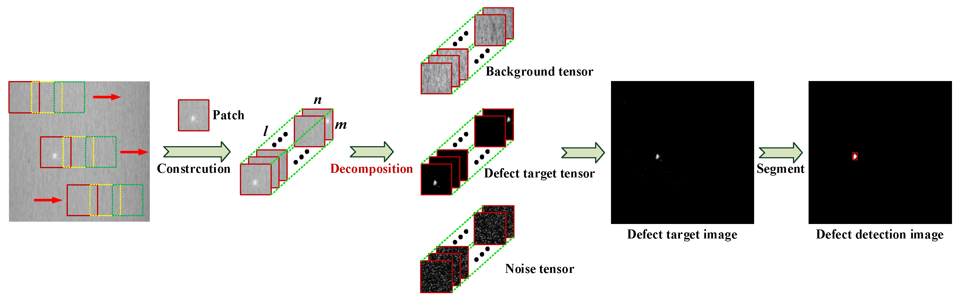
3.1. Construction of Tensor Model for Defect Image

Tensor can be expanded into matrix along n-modes and its i-th frontal slice are denote as X i . We denote X ¯ R n 1 × n 2 × n 3 as the result of Discrete Fourier Transformation (DFT) along its third dimension by using X ¯ , that is, X ¯ = f f t X , [ ] , 3 . The inverse operator computes X from X ¯ , that is, X = f f t X ¯ , [ ] , 3 . The tensor nuclear norm is defined as X * = i = 1 r S i , i , j = 1 n 3 i = 1 r j = 1 n 3 S ¯ i , i , j , where, r = r a n k t X , and S ¯ i , i , 1 are the entries on the diagonal of the first slice of S ¯ , which has a decreasing order property. And we denote the l0 norm, the l1 norm and the Frobenius norm of as X 0 , X 1 , X F , respectively.
In defect image, the small defect targets will often be submerged in the background clutter, with low SNR. The target image carries very little information, causing difficulty of target detection. Such defect image data are mainly composed of defect target, the background, and noise, which can be expressed as
f D = f T + f B + f N
where, f D , f T , f B , and f N represent the input of original defect image, defect image, background image, and noise defect, respectively.
The original gray image of small defect target belongs to two-dimensional data, and the two-dimensional gray image will be converted to tensor data structure. Assuming the gray image is D and the tensor structure obtained after data reconstruction is D . The whole image shall be browsed by sliding window, the small patch obtained each time as the obverse side slice of D is shown in Figure 2.
Specific reconstruction steps are as follows:
(i) The sliding window’s size and step length are m × n and k , respectively. The image I is browsed from left to right and from top to bottom. The image patch with size of m × n is an obverse side slice in tensor data.
(ii) After ergodicity, assume the total sliding times of window is l . The obverse side slice obtained by image small patch constitutes the patch tensor D R m × n × l .
The tensor model of defect image can be constructed as follow:
D = T + B + N
where, D , T , B , and N represent the surface defect patch tensor, defect target patch tensor, background patch tensor, and random noise, respectively.
Target patch-tensor T: For defect image from the strip steel production line, defects with fewer pixels with respect to the whole image, it’s sparse compared to the large background regions. Thus, the surface defect image can be considered as a sparse matrix, which makes the corresponding defect target patch-tensor is an extremely sparse tensor, which can be depicted as:
T 0 d
where, d is an integer that is related with defect target characteristics of number and size.
Background patch-tensor B: As illustrated in Figure 1, the gray-value of normal area in defect image is considered to be uniform, which means that the local and non-local patches are highly correlated with each other even though the pixel distance between two patches may be large in an image.
Actually, the mode-1, mode-2 and mode-3 unfolding matrices of the background patch-tensor are also low-rank. In Figure 3 (b)-(d), the singular values convergence characteristics of all the unfolding matrices decline into approximate zero rapidly, which demonstrates that every unfolding mode of the background patch-tensor is intrinsically low-rank. Based on this property, we can consider the background patch-tensor B as a low-rank tensor, and their unfolding matrices are also all low-rank defined as:
r a n k B 1 r 1 r a n k B 2 r 2 r a n k B 3 r 3
where, B 1 , B 2 , and B 3 represent the background patch tensor’s model-1, model-2, and model-3 unfolding matrices, respectively; r 1 , r 2 , and r 3 are positive numbers that constrains the complexity of the background image, the larger the value is, the more complex the background is
Noise patch-tensor N : The noise is usually modeled as additive white Gaussian noise, and it satisfies N F 2 δ , where, δ > 0 denotes the Gaussian noise level.
Based on above analysis, the small white-spot defects detection on galvanized strip steel based on tensor decomposition can be formulated as the following optimization problem:
min T , B , N r a n k B + λ T 0 + η N F 2 s . t . D = B + T + N
where, r a n k represents the matrix rank and 0 represents the 0 norm that indicates the number of non-zero elements in matrix, F 2 indicates F normal which is used to depict the random noise.; λ , η represent the regularization parameter that indicates the sparse error and random noise, which are used to adjust the low-rank characteristics and sparse characteristics.
In general, weights are inversely correlated to singular values, since the larger values help retain the edges in the background area and should be less regularized, weights are inversely proportional to singular values. A reweighted strategy is always added to recover the low-rank and sparse tensor of existing noise and clutter. The empirical results show that the weighted nuclear norm minimization (WNNM) based methods outperform the nuclear norm minimization (NNM) to some extent. Nevertheless, it still suffers from the over-shrinkage problem as the same as NNM. Both NNM and WNNM are actually special cases of weighted Schatten p-norm minimization (WSNM) [31,32]. The principle of WSNM is to assign different weights to different singular values. WSNM has been validated in theory and experiments that it can recover the low-rank component more accurately than WNNM and NNM by adjusting power p to a more suitable value, which can also be applied to separate target from background. Therefore, we incorporate the WSNM as low-rank regularization for improving the accuracy of low-rank and sparse tensor decomposition framework. Thus, we need to generalize the definition of WSNM for tensor, which can be defined as below:
B W p = 1 n 3 i = 1 r j = 1 n 3 W i , i , j S ¯ i , i , j p 1 p
where, n 3 is the number of patches, W i , i , j = ξ n 1 n 2 S ¯ i , i , j + E B denotes a weight tensor, which is defined in Algorithm 1; S ¯ : , : , j represents the singular values of B : , : , j , ξ is a tunning parameter, E is a positive constant.
In order to solve the model, l2,1-norm replaces l0 -norm for relaxation processing. Hence, the convex optimization model is finally solved as follows:
min T , B , N B W p + λ T 2,1 + η N F 2 s . t . D = B + T + N

3.2. Model Solution

In order to solve the Equation (7), the ADMM are selected to solve the separable convex optimization problem. The Lagrange function can be constructed as shown in Equation (8), which can be converted to Equation (9), where Y R r × r × n 3 , μ , and represent the Lagrangian multiplier tensor, penalty factor and inner product among tensors, penalty factor and inner product among tensors.
O B , T , N , Y , μ = B W p + λ T 2,1 + η N F 2 + μ 2 D B T N F 2 + Y , D B T N
O B , T , N , Y , μ = B W p + λ T 2,1 + η N F 2 + μ 2 D B T N + Y μ F 2
Based on ADMM, O can be broken into several sub-problems for iterative update.
(i) Fixation of the rest of the variables and update of B , which is defined by Equation (10).
B k + 1 = arg min B 1 2 D T k N k + Y k μ k B k F 2 + 1 μ k B W p
The Generalized Soft-Thresholding (GST) [33] is incorporated into tensor singular value thresholding (t-SVT) as follows:
B k + 1 = F 1 μ k D T k N k + Y k μ k
where, F denotes solving WSNM-tensor problem, and the detailed process is given in Algorithm 1. k represents the value of variables in k-th iteration.
Algorithm 1: Solving Equation (11)
Input: X R n 1 × n 2 × n 3 , power p
Output: F λ X
step 1: Conduct FFT operation: X ¯ = f f t X , [ ] , 3
step 2: Conduct SVD operation on each frontal slice X ¯ i of X ¯ :
for i = 1 , 2 , , n 3 + 1 2 do
U , Σ , V = s v d X ¯ i , Σ = d i a g σ 1 , , σ r
Compute w = w 1 , w 2 , , w r
for j = 1,2 , , r do
δ i = G S T σ i , λ w i , p ;
end for
Σ = d i a g δ 1 , , δ r , W ¯ i = U Σ V T ;
end for
for i = n 3 + 1 2 + 1 , , n 3 do
W ¯ i = c o n j W ¯ n 3 i + 2 ;
end for
step 3: Compute F X = i f f t W ¯ , [ ] , 3
(ii) Fixation of the rest of the variables and update of T , which is confirmed by Equation (12).
T k + 1 = arg min T λ T 2,1 + μ k 2 D B k + 1 N k + Y k μ k T F 2
As l 2,1 -norm of T is defined as the sum of l 2 -norm of each mode-2 fiber, we matricize each tensor along the 2nd mode, so T k + 1 2,1 = T 2 k + 1 2,1 . It can be transformed into the matrix form with Equation (13).
T 2 k + 1 = arg min T 2 λ T 2 2,1 + μ k 2 D 2 B 2 k + 1 N 2 k + Y 2 k μ k T 2 F 2
Let X = D 2 B 2 k + 1 N 2 k + Y 2 k μ k , so
T 2 k + 1 = arg min T 2 λ T 2 2,1 + μ k 2 X T 2 F 2
According to [34], it has the following close-form solution with Equation (15), where X : , j represents the j-th column of the matrix X .
T 2 k + 1 : , j = X : , j 2 λ μ k X : , j 2 X : , j ,     i f   X : , j 2 > λ μ k 0 ,                                                                   o t h e r w i s e
After T 2 k + 1 is solved, it can be transformed into tensor form T k + 1 .
(iii) Fixation of the rest of the variables and update of N is obtained by Equation (16).
N k + 1 = arg min N η N F 2 + μ k 2 D B k + 1 T k + 1 + Y k μ k N F 2
Differentiating it with respect to N , and let it to be zero:
2 η N μ k D B k + 1 T k + 1 + Y k μ k N = 0
Then, we have
N k + 1 = μ k 2 η + μ k D B k + 1 T k + 1 + Y k μ k
(iv) Fixation of the rest of the variables and update of Y
Y k + 1 = Y k + μ k D B k + 1 T k + 1 N k + 1
(v) Update of μ
μ k + 1 = min ρ μ k , μ m a x
where 0 < ρ < 1 , μ m a x = 10 5 .
(vi) Inspection of termination condition
D B k + 1 T k + 1 N k + 1 F D F < ε
where 10 3 < ε < 10 5 .
The empirical condition r a n k t T k + 1 = r a n k t T k can help reduce the computational time, and its effectiveness has been validated in the experiments. Finally, we summarize the algorithmic process of the proposed SLRTD method in Algorithm 2.
From target-background separation, the tensor D is decomposed into the defect target T and background B . As the sliding step is less than the window size, and then the small block will overlap in replacement. To eliminate the possible artefacts at the patch borders, we use the mean filter to handle with the overlapping area. The defect target image f T and background image f B are reconstructed from T and B , respectively. Finally, the defect targets can be extracted and segmented by the adaptive thresholding segmentation method.
Algorithm 2: Solving Equation (7) by ADMM
Input: Original defect image sequence tensor D R ^ ( m × n × l ) , power p, λ , η
Output: B , T , N
Initialize: D , T 0 = B 0 = N 0 = 0 , W = I , Y = 0 , μ m a x = 10 5 , ρ = 1.1 , k = 0
While: not converged, do
step 1: Update B k + 1 by Equation (11)
step 2: Update T k + 1 by Equation (15)
step 3: Update N k + 1 by Equation (16)
step 4: Update Y k + 1 by Equation (19)
step 5: Update μ k + 1 by Equation (20)
step 6: Check the convergence condition
step 7: Update k = k + 1
end while

3.3. Model Analysis

3.3.1. Computational Complexity

For surface defect image D, it could be constructed into the tensor D R m × n × l with sliding window’s size m × n and times l. The complexity of computing is mainly depending on the optimization of B , which includes three parts: FFT operator, SVD and GST. The computation complexity of FFT operation is O A m n l l o g l , and A represents number of iterations in Algorithm 1. For SVD operators, t-SVT can reduce its number of calculations in half, i.e., only l + 1 2 times. Therefore, the cost of this part is O A m n 2 l + 1 2 . The GST algorithm costs O B m n , and B denotes the number of iteration for GST. In conclusion, the whole complexity of updating B is O A m n l l o g l + A m n 2 l + 1 2 + B m n . For updating T , the computational cost is O m n . Therefore, the whole computational cost of optimizing variables is O C A m n l l o g l + A m n 2 l + 1 2 + B m n + m n , where C is the number of iterations in ADMM.

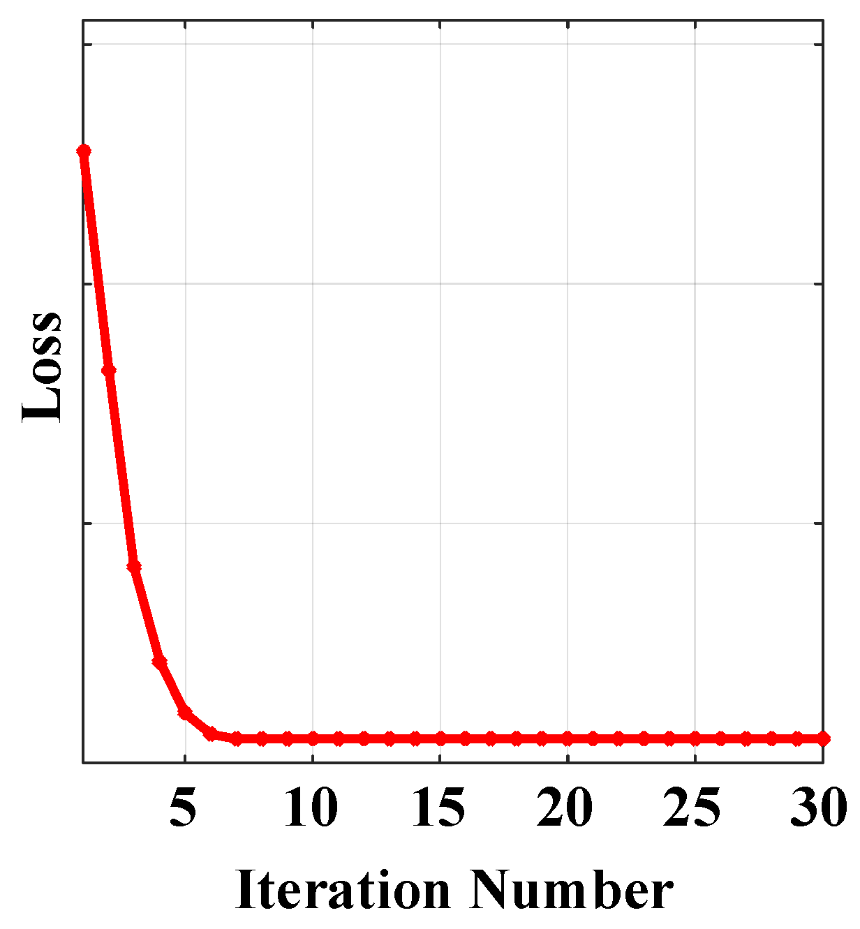
3.3.2. Convergence of Algorithm

The convergence of model Equation (9) has been proven in [25]. We evaluate the convergence of the proposed SLRTD method to empirically show the convergence through experiments in different iterations. We set a convergence error value of D B T N F / D F and found that the algorithm takes approximately 0.5 seconds per frame for small target detection. Figure 4 shows the variation in convergence error as the number of iterations progresses from 0 to 30. It can be observed that after 10 iterations, the error of our algorithm gradually decreases, and the convergence curve stabilizes, indicating that our method meets the convergence requirements and successfully achieves optimal or near-optimal solutions

4. Experiment

To fully verify the effectiveness of the proposed SLRTD method, we conduct a series of qualitative and quantitative experiments. The details of data collection and preprocessing, evaluation metrics are firstly introduced. Secondly, the influence of the key parameters used in our model is analyzed. Finally, four baseline methods are included for performance comparison.

4.1. Experimental Setup

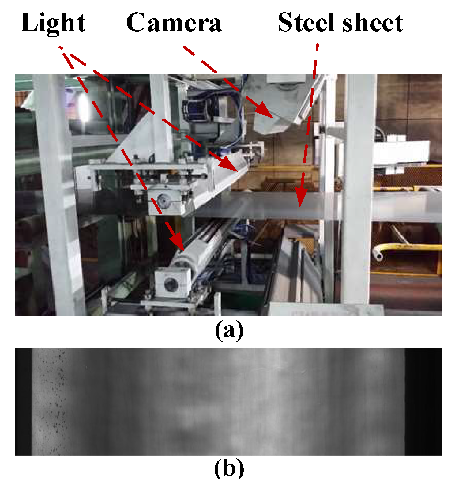
4.1.1. Data Collection and Preprocessing

The proposed SLRTD method is validated on a dataset from real-world galvanized strip steel production line, and the image acquisition platform can be observed in Figure 5. Considering the calculation speed and to ensure the generalization of the model, we crop the raw images 4096×1024 pixels into 200×200 pixels to make the dataset. In total, we get 100 defect images and 100 non-defect images. For each image, the pixel-level ground truth is manually marked by using “1”to denote defective pixels and “0” to denote defect-free pixels. The size of the white-spot defect in the production line is about 1 mm to 3 mm, which is about 5 to 8 pixels in the image with the 200×200 resolution. Defect samples and the corresponding masks of the constructed datasets are shown in Figure 6.

4.1.2. Evaluation Metrics

In order to evaluate the performance of the proposed SLRTD model on defect inspection. The Precision, Recall, precision-recall (P-R) curve, receiver operating characteristic (ROC) curve, area under ROC curve (AUC) and mean square error (MAE) are adopted as evaluation metrics.
Precision is used to evaluate how many pixels, which are predicted positive, are correctly classified, and is calculated by:
P r e c i s i o n = T P T P + F P
where, true positive ( T P ) means the number of defect pixels which are correctly classified into defect categories, false positive ( F P ) indicates the number of background pixel mistakenly identified as defect.
Recall is used to evaluate how many pixels of the same class are correctly classified, and is calculated by:
R e c a l l = T P T P + F N
where, false negative ( F N ) means the number of defect pixels which are not classified to their actual defect class.
Accuracy is used to show the percentage of all the correctly classified pixels, and is calculated by:
A c c u r a c y = T P + T N P + N
where, true negative ( T N ) means the number of non-defect pixels which are correctly classified into background, and P + N (Positive+Negative) is the total number of pixels of the defect image.
M A E = i = 1 H j = 1 W B W i j G i j H × W
where, H and W denotes height and width of surface defect image.
Using Otsu’s threshold, we determine the Precision and Recall by changing thresholds from 0 to 255 to obtain pairs of Precision and Recall.

4.2. Validation of the Proposed Method

4.2.1. Parameter Analysis

The parameters in our model have a key influence on defect target detection performance. The regularized parameter represents the influence of defect target patch-tensor, and it is set to λ = l max m , n , which is adaptive to the patch size of the input image, and number of patches. For the proposed SLRTD method, the patch size, sliding step size and power p are very important parameters which usually affect its robustness. In this subsection, we evaluate the effects of the three parameters by the AUC and MAE on defect images. It should be noted that the performances obtained by changing one of the parameters with the others fixed may not be globally optimal.
a. Patch size
From the perspective of detection performance, we want the patch size to be as large as possible to improve the sparsity and low-rank of small target. However, the larger patch size would also increase the computational complexity simultaneously. To balance the detection performance and computational complexity, we vary the patch size from 20 to 50 with 10 intervals and give the corresponding AUC and MAE in Table 1. As the patch size increases, the overall detection probability of proposed SLRTD method tends to decrease. The degradation is more serious especially when the patch size is 50×50. It is because that the larger patch size would destroy the correlation between the non-local patches, affecting the separation of targets and backgrounds
b. Step size
The choice of sliding step also impacts the patch image size. In practice, we hope to take a larger step in exchange for the reduction of computational complexity. In this experiment, we fix the patch size and vary the step size from 10 to 40 with 10 intervals. The evaluation results are shown in Table 1. It could be observed that the performances of larger steps are always better than that of smaller ones, but when the step size is similar with the patch size, the performance becomes worse.
c. Value of Schatten-p
The WSNM is adopted in our model to solve the over-shrink problem of the low rank estimation, and power p is a decisive factor. Table 2 shows the AUC and MAE on defect datasets with p varying from 0.4 to 1 with 0.3 intervals. The performance of p = 1 is worse than the results of p = 0.7 and p = 0.4 , since the over-shrinkage problem is serious in this case, which validates the effectiveness of WSNM. With p decreasing, the low-rank components can be closer to true rank, while more high rank components would become zeros. However, the performance is not good when p = 0.7 , since too small p would also make some low-rank components become zeros, which also degrade the accuracy of estimation. Therefore, we set p = 0.7 in the following experiments.
.

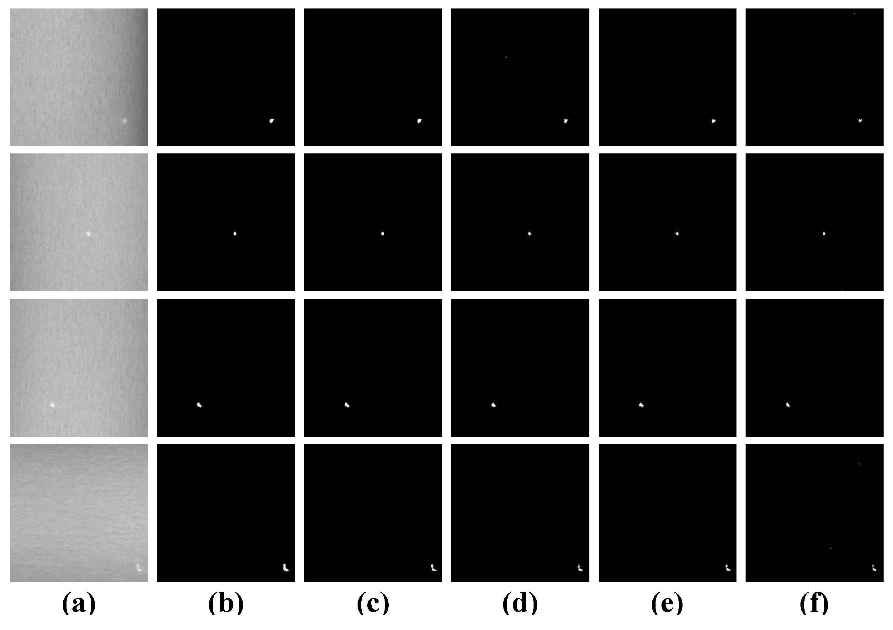
4.2.2. Robustness to Noise

The noise conditions of real factories are complex and random, thus the robustness to noise is very vital in evaluating small defect target detection method. Here we evaluate the proposed SLRTD method’s performance in the noise case with different levels. Additive Gaussian noise with different signal to noise ratio (SNR) is introduced to the original defect image, including 36dB, 32dB, and 28dB. The experimental results are shown in Figure 7 and Table. 3. It could be observed that the SLRTD is robust to noise in most cases, binarization defect images obtained by SLRTD are clear and accurate. When SNR decreases gradually, the AUC and MAE metrics can remain a relative high level, for example, AUC still remain around 0.85 under the condition of S N R = 28 d B , which is considered as less sensitive to noise. However, there are still a few cases that the small targets could not be detected accurately, for example, some pixels of background are misclassified for defect. We think this failure is acceptable, since the small target is totally overwhelmed by the noise. Therefore, it is difficult for SLRTD to discriminate the noise from target, and the detection of small defect target under heavy noise is still a great challenge.

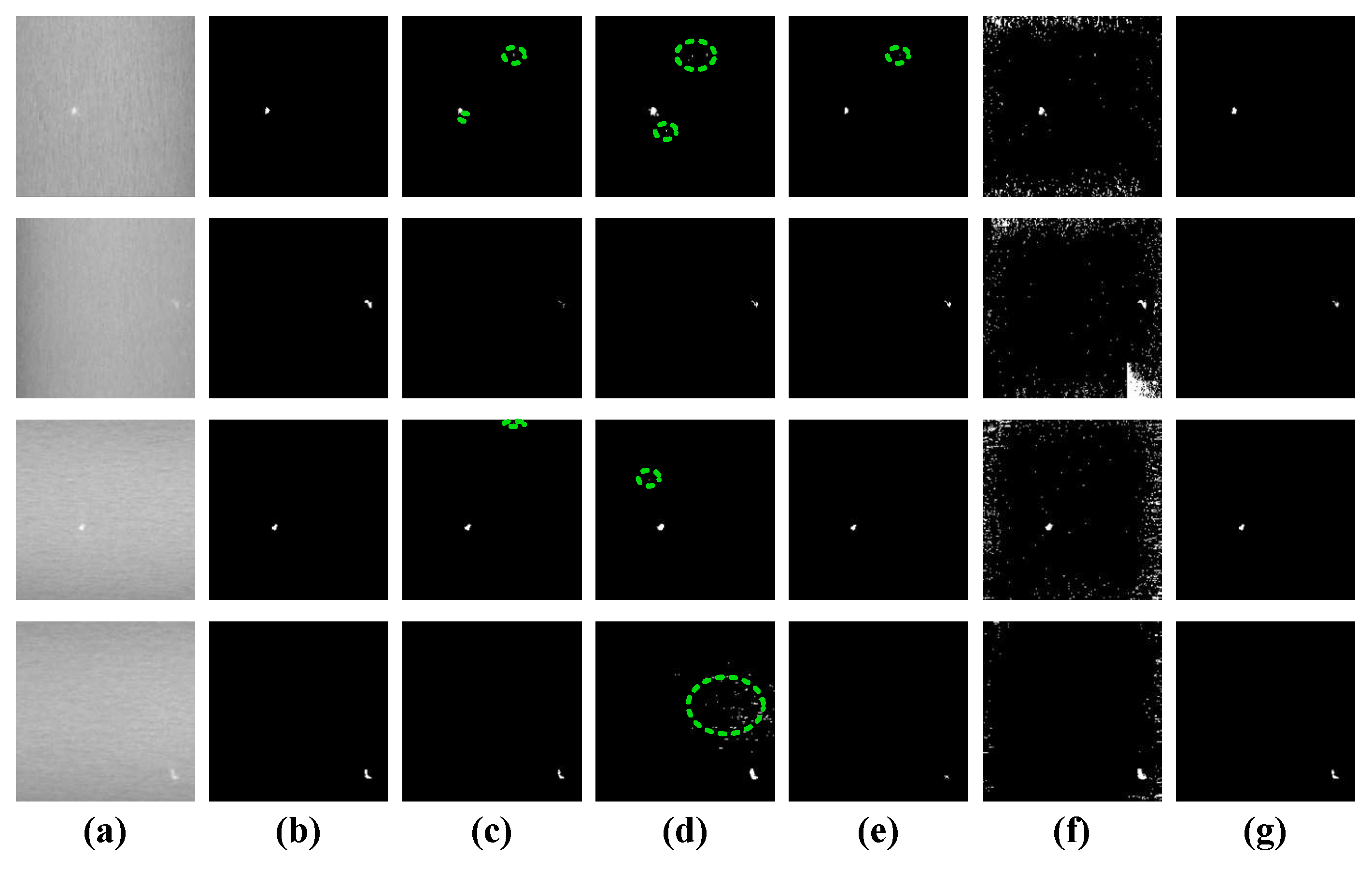
4.3. Comparison with the State-of the-Art Methods

The proposed SLRTD method is compared with four state-of-the-art algorithms, including TRPCA [23], PSTNN [24], ETRPCA [25], and NN-TRPCA [29]

4.3.1. Qualitative Comparison

To facilitate a more intuitive comparison of the performance of each algorithm, we selected representative defect image from the dataset. The false detected targets are highlighted with green circle, which are shown in Figure 8. The qualitative comparison results between the proposed SLRTD method and other four methods are shown in Figure 8. These images are various illumination and gray levels. NN-TRPCA and PSTNN could enhance defect targets, but it also enhances many clutters and noises of background and the defect object could not be uniformly highlighted, which would cause high false alarm rate. These methods may lose the targets with heavy noise. NN-TRPCA exhibits poor robustness in detecting small targets against complex backgrounds, resulting in considerable background residue. TRPCA and ETRPCA method can suppress most of the clutters and detect the targets in 2nd, 4th row, but it still remains some background residuals. There are many pixels that belonging to the background are misjudged by defect, which leads to low accuracy. By contrast, SLRTD separates the defect objects from the image background successfully and locates various defects precisely. It more efficiently highlights the whole defect object with well-defined boundaries than the other methods. It can be concluded from the difference of the results between ETRPCA and SLRTD that WSNM regularization could improve the performance. Besides, WSNM regularization of SLRTD contributes to the good performance, and thus, is the important factor to obtain more precise segmentation results than other methods. What’s more, it’s reasonable to conclude that treat the matrix singular values differently by which the most important characteristics of defects or background can be preserved
The superiority of the proposed SLRTD method is shown in comparison with other competitive approaches, which could suppress the clutters and noise clearly and detect the targets, which can generate high-quality binary segmentation results by simple threshold method.

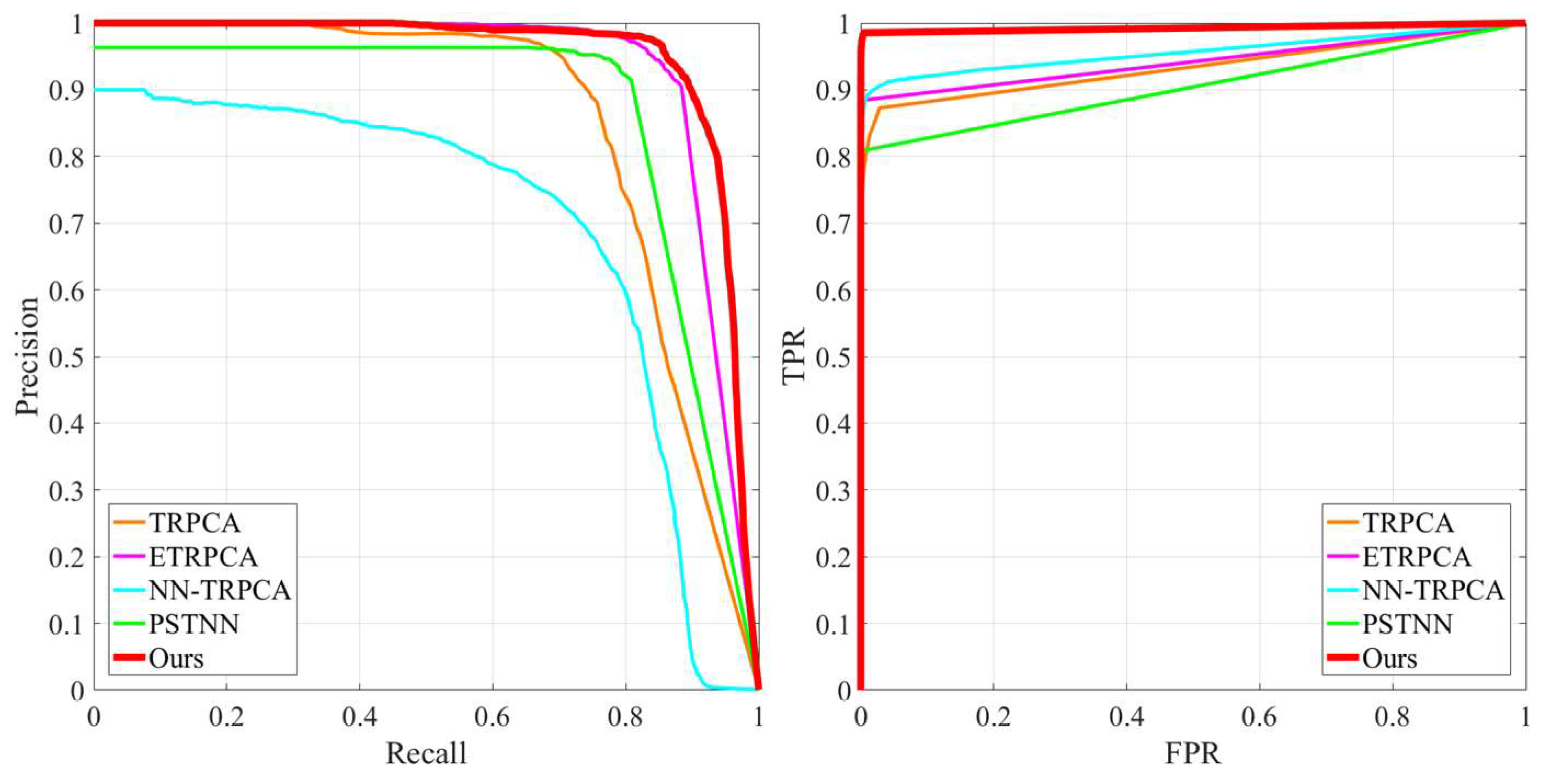
4.3.2. Quantitative Comparison

To further demonstrate the superiority of the proposed SLRTD method, the P-R and ROC curves are displayed in Figure 9. Here, we take four competitive methods TRPCA, ETRPCA, NN-TRPCA, PSTNN for comparison. It could be observed that for the same false alarm ratio, our method can achieve the highest detection probability compared with other methods in most cases, meaning that it has the best performance. By imposing p-norm to the patch-image, SLRTD can suppress backgrounds effectively for all defect image and lay a good foundation for the subsequent target segmentation. Table 4 summarizes the quantitative results of five methods, and the best results are marked in bold. It demonstrates that SLRTD also has better performance than other four methods. Most of AUC results are higher than 85%, and SLRTD achieves 0.9560. MAE of SLRTD is typically the lowest among all the methods. Compared with TRPCA, it’s increased by 2.08% and 1.55% in AUC and MAE, respectively. Based on the above qualitative and quantitative analyses, it confirms that our proposed SLRTD method consistently outperforms some state-of-the-art methods and verifies the effectiveness of the proposed SLRTD method.

5. Conclusion

In order to accurately and rapidly and detect small white-spot defect of surface of galvanized strip steel, the SLRTD method is proposed in the paper. The nonlinear reweighting strategy based on Schatten p-norm are adopted to separate the defect image into smooth non-defect background and random noise. A solution framework is proposed by ADMM algorithm to obtain the defect target image. Based on the self-constructed defect dataset, experiments are conducted by the qualitative and quantitative method, which achieves the best performance among the state-of-the-art defect detection methods. In the future, we will focus on improving the ability of the proposed SLRTD method to detect the other tiny defect under weak illumination conditions or irregular defect-like textures surfaces. In addition, more three-dimensional information about the surface defect through binocular and structured-light stereo vision, which can provide more feedback and reference for industrial production.

Author Contributions

Shiyang Zhou designed the SLRTD model and performed the evaluation experiments. Xuguo Yan collaborated closely and contributed valuable comments and ideas. Huaiguang Liu arranged the datasets, as well as reviewed the article. Caiyun Gong developed the automatic optical inspection procedure. All authors contributed to writing the article.

Funding

This research was funded by National Natural Science Foundation of China, grant number 52205537 and 51805386, the open fund of State Key Laboratory of Intelligent Manufacturing Equipment and Technology (Huazhong University of Science and Technology), grant number IMETKF2025024, the Innovative Research Group Project of National Natural Science Foundation of Hubei Province of China, grant number 2024AFA026.

Institutional Review Board Statement

Not applicable.

Informed Consent Statement

Not applicable.

Data Availability Statement

The data are not publicly available due to privacy issues.

Acknowledgments

The authors would like to thank the editor and anonymous reviewers for their helpful comments and suggestions.

Conflicts of Interest

The authors declare no conflicts of interest.

References

  1. Diers, J.; Pigorsch, C. A survey of methods for automated quality control based on images. INT. J. COMPUT. VISION 2023, 131, 2553–2581. [Google Scholar] [CrossRef]
  2. Zhu, J.P.; He, G.H.; Zhou, P. MFNet: a novel multilevel feature fusion network with multibranch structure for surface defect detection. IEEE T. INSTRUM. MEAS. 2023, 72, 1–11. [Google Scholar] [CrossRef]
  3. Cheng, G.; Yuan, X.; Yao, X.W.; Yan, K.B.; Zeng, Q.H.; Xie, X.X.; Han, J.W. Towards large-scale small object detection: survey and benchmarks. IEEE T. PATTERN. ANAL. 2023, 45, 13467–13488. [Google Scholar] [CrossRef]
  4. Li, J.; Wu, R.; Zhang, S.; Chen, Y.L.; Dong, Z.C. FASCNet: an edge-computational defect detection model for industrial parts. IEEE INTERNET. THINGS. 2023, 11, 6622–6637. [Google Scholar] [CrossRef]
  5. Luo, Q.W.; Chen, Y.W.; Su, J.J.; Yang, C.H.; Silvén, O.; Liu, L. Prior-guided YOLOX for tiny roll mark detection on strip steel. IEEE SENS. J. 2024, 24, 15575–15587. [Google Scholar] [CrossRef]
  6. Ameri, R.; Hsu, C.C.; Band, S.S. A systematic review of deep learning approaches for surface defect detection in industrial applications. ENG. APPL. ARTIF. INTEL. 2023, 130, 107717. [Google Scholar] [CrossRef]
  7. Khanam, R.; Hussain, M.; Hill, R.; Allen, P. A comprehensive review of convolutional neural networks for defect detection in industrial applications. IEEE ACCESS 2024, 12, 94250–94295. [Google Scholar] [CrossRef]
  8. Zou, Z.X.; Chen, K.Y.; Shi, Z.W.; Guo, Y.H.; Ye, J.P. Object detection in 20 years: a survey. P. IEEE 2023, 111, 257–276. [Google Scholar] [CrossRef]
  9. Jha, S.B.; Babiceanu, R.F. Deep CNN-based visual defect detection: survey of current literature. COMPUT. IND. 2023, 14, 103911. [Google Scholar] [CrossRef]
  10. Liu, G.H.; Chu, M.X.; Gong, R.F.; Zheng, Z.H. Global attention module and cascade fusion network for steel surface defect detection. PATTERN RECOGN. 2024, 158, 110979. [Google Scholar] [CrossRef]
  11. Zare, A.; Ozdemir, A.; Iwen, M.A.; Aviyente, S. Extension of PCA to higher order data structures: an introduction to tensors, tensor decompositions, and tensor PCA. P. IEEE 2018, 106, 1341–1358. [Google Scholar] [CrossRef]
  12. Sun, Y.; Yang, J.G.; An, W. Infrared dim and small target detection via multiple subspace learning and spatial-temporal patch-tensor model. IEEE T. GEOSCI. REMOTE. 2020, 59, 3737–3752. [Google Scholar] [CrossRef]
  13. Yu, Q.; Yang, M. Low-rank tensor recovery via non-convex regularization, structured factorization and spatio-temporal characteristics. PATTERN RECOGN. 2023, 137, 109343. [Google Scholar] [CrossRef]
  14. Wang, M.H.; Hong, D.F.; Han, Z.; Li, J.X.; Yao, J.; Gao, L.R.; Zhang, B.; Chanussot, J. tensor decompositions for hyperspectral data processing in remote sensing: a comprehensive review. IEEE GEOSC. REM. SEN. M. 2023, 11, 26–72. [Google Scholar] [CrossRef]
  15. Luo, Y.; Li, X.R.; Chen, S.H. 5-D spatial-temporal information-based infrared small target detection in complex environments. PATTERN RECOGN. 2024, 158, 111003. [Google Scholar] [CrossRef]
  16. Zeng, N.Y.; Wu, P.S.; Wang, Z.D.; Li, H.; Liu, W.; Liu, X.H. A small-sized object detection oriented multi-scale feature fusion approach with application to defect detection. IEEE T. INSTRUM. MEAS. 2022, 71, 3507014. [Google Scholar] [CrossRef]
  17. Wen, X.; Shan, J.; He, Y.; Song, K. Steel surface defect recognition: a survey. COATINGS 2024, 37, 1–30. [Google Scholar] [CrossRef]
  18. Li, D.; Li, Y.; Xie, Q.; Wu, Y.; Yu, Z.; Wang, J. Tiny defect detection in high-resolution aero-engine blade images via a coarse-to-fine framework. IEEE T. INSTRUM. MEAS. 2021, 70, 1–11. [Google Scholar] [CrossRef]
  19. Zhang, H.Y.; Li, M.; Miao, D.Q.; Pedrycz, W.; Wang, Z.G.; Jiang, M.H. Construction of a feature enhancement network for small object detection. PATTERN RECOGN. 2023, 143, 109801. [Google Scholar] [CrossRef]
  20. Hou, X.Q.; Liu, M.Q.; Zhang, S.L.; Wei, P.; Chen, B.D. CANet: contextual information and spatial attention based network for detecting small defects in manufacturing industry. PATTERN RECOGN. 2023, 140, 109558. [Google Scholar] [CrossRef]
  21. Yang, B.Y.; Liu, Z.Y.; Duan, G.F.; Tan, J.R. Residual shape adaptive dense-nested Unet: redesign the long lateral skip connections for metal surface tiny defect inspection. PATTERN RECOGN. 2023, 147, 110073. [Google Scholar] [CrossRef]
  22. Dai, Y.; Wu, Y.Q. Reweighted infrared patch-tensor model with both nonlocal and local priors for single-frame small target detection. IEEE J-STARS. 2017, 10, 3752–3767. [Google Scholar] [CrossRef]
  23. Lu, C.Y.; Feng, J.S.; Chen, Y.D.; Liu, W.; Lin, Z.C.; Yan, S.C. Tensor robust principal component analysis with a new tensor nuclear norm. IEEE T. PATTERN ANAL. 2019, 42, 925–938. [Google Scholar] [CrossRef] [PubMed]
  24. Zhang, L.D.; Peng, Z.M. Infrared small target detection based on partial sum of the tensor nuclear norm. REMOTE SENS-BASEL 2019, 11, 382–392. [Google Scholar] [CrossRef]
  25. Gao, Q.X.; Zhang, P.; Xia, W.; Xie, D.Y.; Gao, X.B.; Tao, D.C. Enhanced tensor RPCA and its application. IEEE T. PATTERN ANAL. 2020, 43, 2133–2140. [Google Scholar] [CrossRef]
  26. Chen, L.; Jiang, X.; Liu, X.Z.; Zhou, Z.X. Logarithmic norm regularized low-rank factorization for matrix and tensor completion. IEEE T. IMAGE PROCESS. 2021, 30, 3434–3449. [Google Scholar] [CrossRef]
  27. Luo, Y.; Li, X.R.; Yan, Y.F.; Xia, C.Q. Spatial-temporal tensor representation learning with priors for infrared small target detection. IEEE T. AERO. ELEC. SYS. 2023, 59, 9598–9620. [Google Scholar] [CrossRef]
  28. Wang, H.L.; Peng, J.J.; Qin, W.J.; Wang, J.J.; Meng, D.Y. Guaranteed tensor recovery fused low-rankness and smoothness. IEEE T. PATTERN ANAL. 2023, 45, 10990–11007. [Google Scholar] [CrossRef]
  29. Geng, X.Y.; Guo, Q.; Hui, S.X.; Yang, M.; Zhang, C.M. Tensor robust PCA with nonconvex and nonlocal regularization. COMPUT. VIS. IMAGE UND. 2024, 243, 104007. [Google Scholar] [CrossRef]
  30. Huang, Z.X.; Zhao, E.W.; Zheng, W.; Peng, X.D.; Niu, W.L.; Yang, Z. Infrared small target detection via two-stage feature complementary improved tensor low-rank sparse decomposition. IEEE J-STARS. 2024, 17, 17690–17709. [Google Scholar] [CrossRef]
  31. Xie, Y.; Gu, S.H.; Liu, Y.; Zuo, W.M.; Zhang, W.S.; Zhang, L. Weighted Schatten p-norm minimization for image denoising and background subtraction. IEEE T. IMAGE PROCESS. 2016, 25, 4842–4857. [Google Scholar] [CrossRef]
  32. Sun, Y.; Yang, J.G.; Li, M.; An, W. Infrared small target detection via spatial-temporal infrared patch-tensor model and weighted Schatten p-norm minimization. INFRARED PHYS. TECHN. 2019, 102, 103050. [Google Scholar] [CrossRef]
  33. Zuo, W.M.; Meng, D.Y.; Zhang, L.; Feng, X.C.; Zhang, D. A generalized iterated shrinkage algorithm for non-convex sparse coding. ICCV. 2013, 217–224. [Google Scholar] [CrossRef]
  34. Xie, D.Y.; Yang, M.; Gao, Q.X.; Song, W. Non-convex tensorial multi-view clustering by integrating l1-based sliced-Laplacian regularization and l2,p-sparsity. PATTERN RECOGN 2024, 154, 110605. [Google Scholar] [CrossRef]
Figure 1. White-spot defects on the surface of galvanized steel sheet: the rightmost is the proportion of defective pixels in the whole image.
Preprints 150910 g001
Figure 2. The flowchart of the proposed SLRTD method for surface defect detection.
Preprints 150910 g002
Figure 3. Illustration of the nonlocal similarity and the low-rank property of background patch-tensors: (a) one representative defect image; (b)-(d) corresponding singular values distributions curve of the mode-1, mode-2, and mode-3 unfolding matrices of background patch-tensors.
Preprints 150910 g003
Figure 4. Convergence curve of the proposed SLRTD method.
Preprints 150910 g004
Figure 5. Industrial image acquisition platform in the galvanized strip steel production line: (a) Strip steel production line; (b) Image captured from the steel surface.
Preprints 150910 g005
Figure 6. 3D maps of defect samples and the corresponding ground-truth.
Preprints 150910 g006
Figure 7. Detection results of binarization by Otsu’s method in different noise case: (a) original image; (b) ground truth; (c) 0dB; (d) 36dB; (e) 32dB; (f) 28dB.
Preprints 150910 g007
Figure 8. Qualitative comparison results: (a) input image; (b) ground-truth image; (c) TRPCA; (d) ETRPCA; (e) NN-TRPCA; (f) PSTNN; (g) Ours.
Preprints 150910 g008
Figure 9. Figure 9. Quantitative comparison results with P-R curves, and ROC curves.
Preprints 150910 g009
Table 1. Experimental results of AUC and MAE with different patch sizes and step sizes.
Patch Step AUC MAE
20×20 10 0.9341 0.0009
20 0.9712 0.0030
30×30 10 0.9501 0.0007
20 0.9728 0.0019
30 0.9775 0.0046
40×40 10 0.9560 0.0005
20 0.9737 0.0017
30 0.9769 0.0034
40 0.9762 0.0034
50×50 10 0.9589 0.0006
20 0.9732 0.0014
30 0.9760 0.0021
40 0.9744 0.0018
50 0.9731 0.0015
Table 2. Experiment of AUC and MAE with Different p
p AUC MAE
0.4 0.9776 0.0017
0.7 0.9560 0.0005
1 0.9050 0.0005
Table 3. Experiment with different noise level.
SNR No Noise 36dB 32dB 28dB
Index
AUC 0.9560 0.9386 0.9058 0.8272
MAE 0.005 0.1610 0.1731 0.1939
Table 4. Comparison of AUC and MAE of different methods.
Method TRPCA ETRPCA NN-TRPCA PSTNN Ours
Index
AUC 0.9352 0.9259 0.9427 0.8925 0.9560
MAE 0.0160 0.0004 0.0071 0.0003 0.0005
Disclaimer/Publisher’s Note: The statements, opinions and data contained in all publications are solely those of the individual author(s) and contributor(s) and not of MDPI and/or the editor(s). MDPI and/or the editor(s) disclaim responsibility for any injury to people or property resulting from any ideas, methods, instructions or products referred to in the content.
Copyright: This open access article is published under a Creative Commons CC BY 4.0 license, which permit the free download, distribution, and reuse, provided that the author and preprint are cited in any reuse.
Prerpints.org logo

Preprints.org is a free preprint server supported by MDPI in Basel, Switzerland.

Subscribe

Disclaimer

Terms of Use

Privacy Policy

Privacy Settings

© 2025 MDPI (Basel, Switzerland) unless otherwise stated