
Submitted:
17 December 2024
Posted:
18 December 2024
You are already at the latest version
Abstract
In this paper, we extend the definition of tensor products from using invertible transformations to utilising right-invertible matrices, exploring the algebraic properties of these new tensor products. On the basis of this new definition, we define the concepts of tensor rank and tensor nuclear norm and investigate their properties, ensuring consistency with their matrix counterparts. We then derive a singular value thresholding (SVT) formula to approximately solve the subproblems in the alternating direction method of multipliers (ADMM), which is a key component of our proposed tensor robust principal component analysis (TRPCA) algorithm. We conduct a complexity analysis of the proposed algorithm, demonstrating its computational efficiency, and apply it to grayscale video denoising and motion detection problems, where it shows significant improvements in efficiency while maintaining a similar level of quality. This work provides a promising approach for handling large-scale data, offering new insights and solutions for advanced data analysis tasks.
Keywords:
tensor robust principal component analysis (TRPCA)
; right invertible matrices
; tensor nuclear norm
; image processing
1. Introduction
Principal component analysis (PCA) is a fundamental technique in data analysis that is widely used for dimensionality reduction and feature extraction. It is particularly effective in uncovering low-dimensional structures in high-dimensional data, which is prevalent in various fields, such as images, text, videos, and bioinformatics. PCA simplifies the complexity of high-dimensional data while retaining trends and patterns by transforming the data into fewer dimensions, which act as summaries of features. This type of data presents several challenges that PCA mitigates: computational expense and an increased error rate due to multiple test corrections when testing each feature for association with an outcome. Despite its computational efficiency and robustness to minor noise, PCA is highly sensitive to gross corruptions or outliers, which are common in real-world datasets. Recent advancements in robust PCA have addressed these limitations, providing more accurate and stable results in the presence of outliers [1,2,3,4,5,6].
To address this limitation, numerous robust variants of PCA have been developed, but many suffer from high computational costs [7,8,9]. Among these robust variants, robust principal component analysis (RPCA) stands out as a significant advancement [1]. RPCA is the first polynomial-time algorithm with strong recovery guarantees [10]. Given an observed matrix , which can be decomposed as , where is low-rank and is sparse, RPCA demonstrates that if the singular vectors of meet certain incoherence conditions, and can be accurately recovered with high probability by solving the following convex optimisation problem:
Here, represents the nuclear norm (the sum of the singular values of L), and denotes the norm (the sum of the absolute values of all entries in E) [1,3]. The parameter is typically set to , which performs well in practice [1]. Algorithmically, this problem can be efficiently solved at a cost comparable to that of PCA [7,9]. Recent research has focused on improving the efficiency and robustness of RPCA, with novel approaches such as nonconvex RPCA (N-TRPCA) and learned robust PCA (LRPCA) showing promising results [6,11].
However, a primary limitation of RPCA is its applicability only to two-way (matrix) data. Real-world data, especially in modern applications, are often multidimensional and represented as multiway arrays or tensors [12,13]. For example, a colour image is a three-way object with column, row, and colour modes, whereas a grayscale video is indexed by two spatial variables and one temporal variable [12]. To apply RPCA, one must first reshape the multiway data into a matrix, a process that often leads to information loss and performance degradation [3,14]. This limitation has prompted researchers to extend RPCA to handle tensor data directly, leveraging its multidimensional structure [6,15]. Such extensions aim to preserve the inherent structures of the data and avoid the pitfalls associated with reshaping, thus improving the robustness and accuracy of RPCA in handling high-dimensional data [16,17].
To address this issue, recent research has focused on extending RPCA to handle tensor data directly, leveraging its multidimensional structure. One notable approach is tensor robust principal component analysis (TRPCA), which aims to precisely recover a low-rank tensor corrupted by sparse errors[3,15]. Lu et al.[15] introduced a new tensor nuclear norm based on the tensor-tensor product (t-product)[18], which is a generalisation of the matrix-matrix product. This new tensor nuclear norm is the convex envelope of the tensor average rank within the unit ball of the tensor spectral norm, providing a strong theoretical foundation for TRPCA[15].
Building upon this work, we propose a novel TRPCA model that utilises a new concept of tensor products defined via right invertible linear transforms. Specifically, we define new tensor products for third-order tensors via right invertible matrices. These new tensor products generalise the concept of tensor products defined by invertible linear transforms and offer several advantages in terms of computational efficiency and robustness.
Our contributions are summarised as follows:
- Motivated by the new tensor product in Reference [19], which is a natural generalisation of the tensor product with invertible linear transforms, such as the t-product and c-product, we rigorously deduce a new class of tensor products for third-order tensors via right invertible linear transforms. These new tensor products generalise existing tensor product definitions and preserve many fundamental properties of the tensor product defined by invertible linear transforms. This forms the foundation for extending models, optimisation methods, and theoretical analysis techniques from t-products to new products with the right linear transforms.
- Novel TRPCA models that leverage new tensor products to increase computational efficiency and robustness are given. Equipped with the tensor nuclear norm, this model provides a more efficient and robust solution for tensor data.
- We provide theoretical guarantees for the exact recovery of low-rank and sparse components via the new tensor nuclear norm. Under certain assumption conditions, the solution to the convex TRPCA model perfectly recovers the underlying low-rank component and sparse component . The recovery guarantees of RPCA[1] fall into our special cases.
- Numerical experiments are presented to validate the efficiency and effectiveness of the proposed algorithms in various applications, including grayscale video recovery and motion detection. Our experiments show the superiority of the new TRPCA over TRPCA on the basis of the c-product.
This paper is organised as follows: Section 2 introduces the necessary background and notation. Section 3 defines the new tensor products and explores their properties. Section 4 presents the TRPCA model and the theoretical guarantees. Section 5 provides numerical experiments and applications. Finally, Section 6 concludes the paper and discusses future directions.
2. Preliminaries
2.1. Notations
Throughout this paper, vectors are denoted by italic lowercase letters such as and , matrices by uppercase letters such as A and B, and tensors by calligraphic capital letters such as and . Scalars are denoted by lowercase letters, such as a. The notation represents the set of tensors over the field , where can be either the field of real numbers or the field of complex numbers . This notation can also be written as when emphasising two particular dimensions.
For a third-order tensor , the -th entry is denoted as or . Let represent the -th tube of , that is, . A slice of a tensor is a two-dimensional section defined by fixing all but two indices. The -th frontal slice is denoted as , the -th horizontal slice is denoted as , and the -th lateral slice is denoted as .
The inner product between matrices A and B in is defined as , where denotes the conjugate transpose of A and denotes the matrix trace. The inner product between tensors and in is defined as . Several norms are used for vectors, matrices, and tensors. The norm of a tensor is defined as . The Frobenius norm is defined as . These norms reduce to the corresponding vector or matrix norms when is a vector or a matrix. For a vector , the norm is defined as . The matrix nuclear norm is defined as .
2.2. Right invertible transform operator
Consider a matrix M of size with . If M is a right invertible matrix, then there exists a matrix N of size such that . When , M, as a right invertible matrix, is an invertible matrix. A right invertible matrix is a matrix with linearly independent rows. One way to construct a right invertible matrix is by removing some rows from an invertible matrix. Let us consider an discrete cosine transform (DCT) matrix C. Suppose that we want to form a new matrix of size by removing the last m rows from the original matrix F, where . This operation is equivalent to truncating the matrix. The resulting matrix will no longer be square and thus does not have an inverse effect in the traditional sense. However, we can find a right inverse G such that where is the identity matrix. In general, the right inverse of a matrix is not unique. To construct G, we can use the Moore-Penrose pseudoinverse. For a given matrix A, its pseudoinverse is defined as provided that is invertible, where denotes the conjugate transpose of A. Therefore, the right inverse G of is given by: Thus, we form a right invertible pair .
Now, we can define two functions to convert between tube tensors and vectors in . The function converts a tube tensor into a vector in , , where is the vector obtained by stacking the elements of in a column vector. The function converts a vector into a tube tensor, , where is the tube tensor obtained by reshaping the vector into a tensor.
Definition 1.
The mode-3 (matrix) product between and an matrix U is defined as
Definition 2.
Let M be a right invertible matrix of size . We define the right invertible operator L on tube tensors as
and its inverse as
where N is the right invertible matrix of M.
Using the functions vec and unvec, we can also express the operators L and R in terms of vector operations
It can be seen that is not equal to the original tensor in general because is not an identity matrix, although is an identity matrix.
3. Definition and Properties of the New Tensor Product
Definition 3
(Face-wise Product[20]). Let and be two third-order tensors. Theface-wise productbetween and is defined as:
Here, and denote the -th frontal slices of and , respectively, which are matrices of sizes and . The product is the standard matrix multiplication.
Definition 4.
Let M be a right invertible matrix of size . We define theright invertible operator Lon two third-order tensors as
and its inverse as
where N is the right inverse matrix of M.
In the following, if no confusion arises, we do not distinguish the right invertible operator L defined by the same matrix M on different tensor spaces.
Proposition 1.
The operator L is surjective (onto), the operator R is injective (one-to-one), and is the identity mapping.
Proof.
To show that L is surjective, we need to show that for any , there exists a such that . Consider . Then, Using the property , the identity matrix, we obtain . Thus, , showing that L is surjective.
To show that R is injective, we need to show that if , then . Assume that . Then, . Applying the operator L to both sides, we obtain . We have . Using the property , we obtain which simplifies to . Thus, . This shows that R is injective.
To show that is the identity mapping, we need to show that for any , . Consider . Using the property , we obtain . Thus, , showing that is the identity mapping.
□
Definition 5.
Let L be the right invertible operator between and , R be its inverse between and . We define thekernelof the right invertible operator L as
Proposition 2.
Let L and R be defined as above; then, we have
where I is the identity map on .
Proof.
First, we show that . Assuming , then , we need to show that there exists an such that . Consider ; then, , since , we have . Therefore,. Thus, , which shows that .
On the other hand, we show that . Assume . Then, there exists an such that . Thus, . By Proposition 1, is the identity mapping, so . Thus, . This shows that .
Therefore, we have . This completes the proof. □
Using the functions and , we can give an equivalent description of the operators L and R in terms of tube tensors
for all and ,
for all and .
Definition 6.
Let L be the right invertible operator defined by matrix M of size between and , R be its inverse defined by matrix N of size between and . Theright invertible transform productfor two third-order tensors and based on is denoted by
and is defined as
If there is no confusion and for simplicity, we denote
Proposition 3.
Let L be the right invertible operator between and , and R be its inverse between and . For and , the -th tube fibre of can be computed as the appropriate sum of tube fibre products; i.e.,
where and are the tube fibres of and , respectively.
Proof.
According to the definition, L maps to and to . Therefore, and By definition, ▵ is a matrix multiplication operation, so Apply R to map the result back from to , we have By definition, is the -th tube fibre of . We can express it as According to the properties of matrix multiplication, the -th element of can be written as Apply R to each term in the sum By the definition of the product, we have Therefore, the -th tube fibre of can be expressed as This completes the proof. □
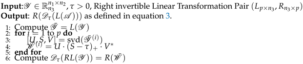
Now, we provide the algorithm for computing the product of two tensors in Algorithm 1.
| Algorithm 1 Compute the product of two tensors |
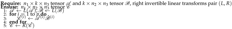 |
The product retains several properties of the tensor product defined via invertible linear transformations[20]. However, owing to the generally noninvertible properties of the right invertible transformation used to define the product, several properties exhibit notable differences.
Lemma 1.
If are third-order tensors of appropriate sizes, then the following statements are true:
- Associative Property:
- Distributive Property:
- Noncommutative Property: In general,
Proof.
Associativity: Let be third-order tensors in ; then, by the linear properties of operators L and R and the fact that is the identity transformation, we have
Distributivity:
Similarly,
Noncommutativity: In general, the product is not commutative. This is because in most cases, leading to . □
The above proof of associativity shows that the transformation is the identity transformation. This also indicates that, under this definition, if L is a left invertible transformation, the associative property does not hold.
Theorem 1.
(Commutativity of the product for tube tensors). If , then the product is commutative. Specifically,
Proof.
Recall the definition of the product, where L is a linear transformation and R is its right invertible transformation. For tube tensors , let be the matrix of the linear transformation L and the right invertible transformation R, respectively; then, . For vectors, the operation ▵ is typically a component-wise multiplication for these vectors. Since component-wise multiplication is commutative, we have
that is, Applying the right invertible transformation R to both sides, we obtain By the definition of the product, this implies Thus, the product is commutative for scalar tensors in . □
Definition 7
( conjugate transpose). Let L be the right invertible operator between and . Theconjugate transposeof a third-order tensor , denoted by , is the tensor obtained by conjugate transposing each of the frontal slices in the transform domain. Specifically,
where denotes the i-th frontal slice of and denotes the conjugate transpose of the i-th frontal slice. However, since L is not necessarily invertible, different tensors may transform into the same tensor. Therefore, the conjugate transpose of is not necessarily unique.
If is the conjugate transpose of , then where is also a conjugate transpose of . This is because for any , we have ; thus, . Therefore, satisfies the same properties as in the transform domain, making it another valid conjugate transpose of .
Proposition 4.
The multiplication reversal property of the conjugate transpose holds: .
Proof.
By definition, we have
The result follows from equality in the transform domain by definition. □
Definition 8
( identity tensor). Let L be the right invertible operator between and . Theidentity tensor is defined such that its frontal slices in the transform domain are all identity matrices. Formally, for ,
where denotes the identity matrix.
It is clear that . It is easy to say that , for all .
Definition 9
( unitary tensor). Let . is said to beunitaryif .
It is clear that if is unitary, then for all is also unitary according to the definition above.
Definition 10
(F-diagonal/F-upper/F-lower tensor). Let L be the right invertible operator between and and . Then, is called anF-diagonal/F-upper/F-lower tensorif all frontal slices of are diagonal/upper triangular/lower triangular matrices in the transform domain.
Having established the requisite algebraic framework, we are equipped to define a product-based tensor singular value decomposition. This formulation closely parallels the L SVD introduced in Reference[20].
Theorem 2
( SVD). Let L be the right invertible operator defined by matrix M of size between and , R be its inverse defined by matrix N of size between and . Let ; then, we have the following SVD:
where and are unitary tensors and is an F-diagonal tensor. The main steps for computing the tensor SVD are summarised in the following algorithm.
Definition 11.
Define the SVD error of the SVD decomposition as where
When L is an invertible linear transformation, the SVD error of the SVD decomposition is a zero tensor.
| Algorithm 2 SVD under the product |
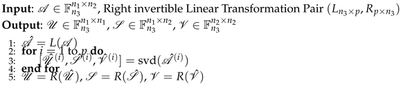 |
Now, we can define the tensor multirank and tubal rank associated with the tensor product and the SVD as follows.
It is known that the singular values of a matrix have a decreasing order property. Let be the SVD of . The entries on the diagonal of the first frontal slice have the same decreasing property, i.e.,
where . This property holds since the matrix N in the definition of the product gives
and the entries on the diagonal of are the singular values.
Definition 12
( tensor multirank and tubal rank). Let L be the right invertible operator defined by matrix M of size between and , R be its inverse defined by matrix N of size between and . Let , the tubal rankof under the product is defined by the number of nonzero tubes of , where is obtained from the SVD, i.e.,
Definition 13
( tensor average rank). For a tensor , the tensor average rankof , denoted as , is defined as
where represents the i-th frontal slice of in the transform domain and L is the right invertible linear transformation used in the definition of the product.
Theorem 3.
Let be an invertible matrix, and let be the matrix formed by retaining the first p rows of . Then, for any tensor ,
with , where is the tubal rankof associated with , .
Note that similar conclusions hold for the tensor average rank.
Theorem 4.
For any tensor , the relationship between the tensor average rank and the tensor tube rank of satisfies
Proof.
Given that the SVD of has k nonzero singular values in , that is, , the inequality of the singular value of each frontal slice decreases. Therefore, for each i, we have:
Summing the above inequality over all i and taking the average, we obtain
Thus, we have
This theorem demonstrates that the tensor average rank is always less than or equal to the tensor tube rank. This relationship indicates that the tensor tube rank can be seen as an upper bound on the average rank of the frontal slices of the tensor. This result is significant in tensor decomposition and low-rank approximation problems, especially in the design and analysis of robust tensor decomposition algorithms.
Theorem 5.
The average rank of a tensor is less than or equal to its CP rank.
Proof.
Assume that the CP decomposition of the tensor is where R is the CP rank Consider the i-th frontal slice of the tensor in the transform domain. According to the CP decomposition, each frontal slice can be expressed as . Since is a linear combination of R rank-1 matrices, the rank of is at most R:
According to the definition of tensor average rank, we have Since each has a rank of at most R, we obtain
Therefore, we have This completes the proof. □
Recall the inequality , we have
Corollary 1.
The average rank of a tensor is less than or equal to its Tucker rank.
These results provide insights into the structure of tensors and are useful in various applications involving tensor decompositions and low-rank approximations.
4. Tensor Robust Principal Component Analysis with Novel Tensor Multiplication
In the field of image processing, the low-rank property of images is an important characteristic. However, the low-rank function is nonconvex and highly sensitive to parameter choices and noise, making the optimisation problem challenging to solve. Because the properties of the rank function are poor, researchers have proposed the use of the nuclear norm, which approximates the tensor rank. This convex relaxation of the tensor rank not only simplifies the optimisation problem but also improves its convergence properties and robustness. In the following, the nuclear norm is defined as a measure that captures the low-rank structure of the tensor after the right invertible linear transformation pair is applied.
4.1. Tensor Nuclear Norm with New Tensor Multiplication
Definition 14.
Let and be a right invertible matrix for defining the product, and then define thenuclear normof under the product as follows:
By this definition, we have for all .
Since both definitions are based on slices, combining the conclusion that the nuclear norm is the convex envelope of the matrix rank, the convex envelope of the tensor average rank in the meaning of the product is the tensor nuclear norm .
The standard alternating direction method of multipliers (ADMM) is used in the process of solving the tensor robust principal component analysis with tensor nuclear norm problem. A crucial step in this process is the computation of the proximal operator of the tensor nuclear norm (TNN).
The optimisation subproblem for the TRPCA can be formulated as follows:
where denotes the tensor nuclear norm based on the product, denotes the Frobenius norm, and is a regularisation parameter.
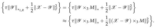
We provide an approximate solution for this optimisation problem[21], which can be interpreted as the proximal operator of the matrix nuclear norm. Let represent the singular value decomposition (SVD) of tensor . For each , we define the tensor singular value thresholding ( SVT) operator as follows:
where
where is the R transformation in the product, which applies the soft-thresholding operation to the frontal slices of the tensor along the k-th dimension. Specifically, for each frontal slice of the tensor , the soft-thresholding operation is given by
Note that represents the singular value tensor obtained from the SVD decomposition of in the transform field. The notation denotes the positive part of r, i.e., . This operator applies a soft-thresholding rule to the singular values of the frontal slices of , effectively shrinking these values towards zero. The SVT operator is the proximity operator associated with the TNN.
This formulation ensures that the solution is a low-rank approximation of the original tensor while maintaining a balance between rank minimisation and the data fidelity term. The SVT operator effectively reduces the rank of the tensor by thresholding the singular values, making it a powerful tool in tensor completion and robust principal component analysis tasks.
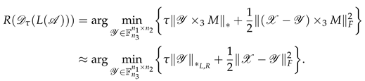
Theorem 6.
Let , , and L be a right inverse linear transformation. Let the matrix representation of L be , which consists of the first p rows of an orthogonal matrix. Then,
where denotes the tensor nuclear norm based on the product, denotes the Frobenius norm, and is a regularisation parameter.
The closed-form expression for the SVT operator is a natural extension of the t-SVT operator[3].
Proof.
By using the properties of the Frobenius norm and the tensor nuclear norm under orthogonal transformations:
and
where and are the matrices and tensors obtained through the orthogonal transformations L and R.
Since L and R are orthogonal transformations, they preserve the Frobenius norm and the nuclear norm, i.e.,
and
Therefore, the original problem can be written as follows:
By Theorem 2.1 in Reference[7], the i-th frontal slice of solves the i-th subproblem of the above minimisation problem. Hence, solves the entire problem. □
Theorem 7.
Let and . Let be the matrix corresponding to L, satisfying , then
where denotes the tensor nuclear norm based on the product, denotes the Frobenius norm, and is a regularisation parameter.
Proof.
Let be the matrix corresponding to the truncated orthogonal transformation L. The condition implies that
 By Theorem 6, we have
□
| Algorithm 3 Tensor Singular Value Thresholding ( SVT) |
 |
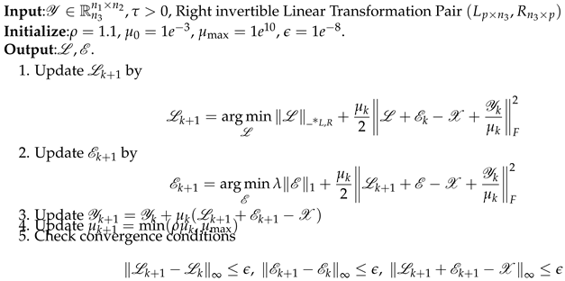
4.2. ADMM Algorithm for Tensor Robust Principal Component Analysis
We consider the following optimisation problem
where is the low-rank tensor; is the sparse tensor; is the observed tensor; is the tensor nuclear norm (low-rank regularisation term); is the tensor norm (sparsity regularisation term); and is the balancing parameter between low-rank and sparsity.
To solve this problem via the alternating direction method of multipliers (ADMM), we introduce the augmented Lagrangian function as follows:
where is the Lagrange multiplier and is the penalty parameter.
The ADMM algorithm updates , , and iteratively.
Update :
Update :
Update :
Convergence Conditions:
where is a small positive tolerance.
In the following, we present the solution of the subproblem in the ADMM.
Solution of Update : Approximate solution of the subproblem to update the low-rank tensor
First, we set
then, the objective function can be rewritten as
This problem can be solved via the tensor singular value thresholding operation , as defined in Equation 3; here, we denote it as t-SVT. The t-SVT operation is defined as
where is the threshold parameter. In our subproblem, and ; thus,
Substituting back , we obtain
Solution of Update : Subproblem 2 can be solved via the soft-thresholding operator
where the soft-thresholding operator is defined as
This operation effectively shrinks the singular values of the tensor towards zero, promoting a low-rank structure in the tensor .
4.3. Computational Complexity Analysis
In this section, we analyse the computational complexity of the proposed method, which uses the alternating direction method of multipliers (ADMM) to solve the tensor robust principal component analysis (TRPCA) problem. The initialisation step, involving the setup of the low-rank component , the sparse noise component , and the penalty term , has a complexity of , where , , and are the dimensions of the tensor. Each ADMM iteration consists of updating by performing singular value decomposition (SVD) on each of the p slices of the transformed tensor, resulting in a complexity of . Updating via soft thresholding has a complexity of , whereas updating and checking the convergence conditions both have a complexity of . Assuming k iterations, the total complexity of the ADMM process is . From the complexity analysis, it is evident that the first dimension p of the right inverse matrix has a linear relationship with the computational complexity.
| Algorithm 4 Solve (5) via ADMM |
 |
5. Numerical Experiments
In this section, we apply the TRPCA algorithm to both randomly generated synthetic data and real-world data for grey video denoising and motion detection. This approach allows us to evaluate the performance of the algorithm and demonstrate its advantages. All the experiments were conducted on a personal computer equipped with an Intel(R) Core(TM) i7-9750H 2.30 GHz processor and 8 GB of RAM. We conduct our experiments via Python. We applied the TRPCA algorithm to recover the original tensor from those corrupted by random noise. To simulate sparse noise interference in real-world applications, we added sparse noise to the original data tensor . Specifically, we first created a zero matrix sparse_noise with the same shape as . Next, we randomly selected 1% of the elements in as noise points, ensuring that each position was chosen only once. For these selected positions, we assigned random values drawn from a uniform distribution . Finally, we added the generated sparse noise matrix sparse_noise to the original data to obtain the noisy data .
We use the peak signal-to-noise ratio (PSNR) for each slice along the third dimension, defined as
To evaluate the recovery performance of each slice, represents the k-th slice along the third dimension of the original tensor data; represents the k-th slice along the third dimension of the recovered tensor data after processing; represents the k-th slice along the third dimension of the observed tensor data, which may contain noise or other distortions; and represents the sizes of the first and second dimensions of the tensor slices. The PSNR is a measure of the quality of the recovered data compared with the original data. Higher PSNR values indicate better recovery performance.
The relative squared error (RSE) for each slice along the third dimension, used to measure the relative error between the recovered data and the original data, is defined as follows:
where represents the mean of the k-th slice along the third dimension of the observed tensor data, i.e., the average value of all the elements at each position in the slice. The RSE measures the relative squared error between the recovered data and the original data. Lower RSE values indicate better recovery performance. We choose the PSNR, relative squared error (RSE), and runtime as the evaluation metrics to assess the denoising performance of various TRPCA methods.
The right invertible matrix is obtained by removing some rows from a discrete cosine transform (DCT) matrix. The size parameter denotes the number of rows retained from the DCT matrix. Specifically, we set the size p to 20, 40, 60, 100, and 200. When the size is 200, it corresponds to the classical TRPCA method, which is based on the c-product[20]. The classical TRPCA method, which is based on the c-product method, outperforms robust principal component analysis (RPCA) and sparse nonnegative matrix factorisation (SNN) by providing better recovery accuracy and noise reduction in the processed data by Reference[15]. Therefore, in our comparative experiments, we only compare different size cases. On the basis of the related literature and our experimental calculations, we set to
5.1. Synthetic Data
In this section, we evaluate the performance of the proposed nuclear norm-based TRPCA method using synthetic data. The synthetic data are generated as a random tensor of dimensions normalised to the range [0, 1]. Sparse noise is added to the original tensor, affecting approximately of the elements. The noisy tensor is then used as input to the TRPCA algorithm. For simplicity, we will use the condition to approximate the analysis of .
The synthetic data are generated as a random tensor of dimensions , normalised to the range [0, 1]. We compute the ratio for different sizes of the right invertible matrix M.
Table 1 shows the computed ratios for different sizes of the right invertible matrix M. These ratios indicate that for artificial random data, the ratio approaches 1 as the size of M increases.
The experiment involves varying the size of the right invertible linear transformation matrix, denoted as p, from 20 to 200 in steps. For each size, the TRPCA algorithm is applied to the noisy tensor, and the results are evaluated via the peak signal-to-noise ratio (PSNR) and relative squared error (RSE) metrics. The PSNR and RSE values are calculated for all frames of the tensor.
The results show that the proposed method effectively recovers the low-rank component of the tensor while maintaining computational efficiency and stability. The PSNR values increase as the size of the right invertible matrix increases, indicating better recovery performance. The RSE values also decrease, confirming the improved accuracy of the low-rank approximation.
Table 2 summarises the runtime of the TRPCA algorithm for different sizes of the right invertible matrix. As the size increases, the runtime also increases, but the improvement in PSNR and reduction in RSE justify the additional computational cost.
5.2 Video Denoising and Anomaly Detection
In these experiments, we used the Test001 subset from the UCSD_Anomaly_Dataset directory. The UCSD anomaly detection dataset is a widely used benchmark for evaluating anomaly detection algorithms in video surveillance. Test001 includes 200 frames from a video sequence, which we used to construct a video tensor. For more information about the dataset, please refer to UCSD Anomaly Detection Dataset.
The video data are represented as a tensor of dimensions . We compute the ratio for different sizes of the right invertible matrix M.
Table 3 shows the computed ratios for different sizes of the right invertible matrix M. These ratios indicate that for real data, the ratio approaches 1 more closely than synthetic data do. This confirms that real data are more consistent with the condition
Figure 3 shows the PSNR values for different sizes across various frames. Figure 4 shows the RSE values for different sizes across various frames. Combining the information from the previous text and the new details about Figure 3 and Figure 4, we can analyse the experimental results as follows.
We can deduce that for most frames, the PSNR values remain relatively close across different sizes, suggesting consistent recovery quality. Interestingly, in certain specific frames, smaller sizes (such as 20 and 40) manage to achieve slightly higher PSNR values than larger sizes (such as 100 and 200), suggesting a possible advantage in terms of recovery performance.
Similarly, Figure 4 shows the relative squared error (RSE) values for different sizes across various frames. Upon examining this figure, we notice that for most frames, the RSE values are relatively close across different sizes, further supporting the notion of consistent recovery quality. Once again, in some specific bands, smaller sizes (e.g., 20 and 40) display slightly lower RSE values than larger sizes (e.g., 200), reinforcing the trend observed in the PSNR analysis.
In Table 4, we present the runtime analysis for the TRPCA method applied to video sequences with different DCT truncation sizes. The DCT truncation sizes considered are 20, 40, 60, 100, and 200. The runtime for each size is measured in seconds. As shown in Table 4, the runtime increases significantly with increasing DCT truncation size. This trend indicates that larger DCT truncation sizes, although providing better recovery performance, come at the cost of increased computational time. Therefore, a trade-off between recovery quality and computational efficiency must be considered when selecting the appropriate DCT truncation size for practical applications.
On the basis of the numerical results, several conclusions can be drawn regarding the impact of varying truncation levels in the definition of the TRPCA algorithm using different-sized right invertible matrices derived from the discrete cosine transform (DCT).
First, in Figure 5, the top row presents the original images from frames 40, 70, and 120, whereas the second row shows the corresponding noisy versions. The other row shows the recovery results achieved via the TRPCA method with a right invertible matrix constructed from the different truncations of the DCT matrix. The bottom row shows the recovery results when the TRPCA approach with a right invertible matrix formed by the top 200 rows of the DCT matrix. In Figure 6, the top row again features the original images from the same set of frames, followed by the noisy versions. The other row shows the residual results after denoising via the TRPCA method with a right invertible matrix constructed from the different truncations of the DCT matrix. Notably, these recovered images are significantly closer to the original images, suggesting that incorporating more DCT coefficients enhances the recovery process, albeit at the cost of increased computational complexity. These figures highlight the varying recovery efficacy across different frames within the video sequence. For example, frame 120, where a child quickly rides a bicycle into the scene, yields less satisfactory recovery results than slower-motion scenes such as frames 40 and 70 do. This observation highlights the impact of anomalous situations on video recovery, particularly how fast movements generally compromise recovery accuracy. Although the recovery results are not as good for larger sizes, this method can still detect anomalous situations effectively.
Nonetheless, adopting larger TRPCA truncation sizes enables superior denoising and recovery outcomes even in regions with rapid motion. Consequently, adjusting the number of DCT coefficients employed in the TRPCA method offers a trade-off between recovery quality and computational efficiency. Specifically, smaller sizes yield higher computational efficiency for frames with slow image transformations, whereas larger sizes enhance recovery quality in the presence of fast-moving objects because of the accelerated pixel variations at the same location, which facilitates dynamic detection.
To optimise both recovery quality and computational efficiency in video sequence denoising and recovery tasks, it is advisable to segment the video according to its motion intensity. Smaller transformation sizes can be applied to sections with slow motion to conserve computation time, whereas larger sizes can be utilised in parts with rapid motion to ensure better precision. This adaptive strategy strikes a balance between the two objectives, ensuring optimal performance tailored to specific application demands.
In light of these findings, it becomes evident that the TRPCA method offers a balance between recovery quality and computational efficiency. Smaller sizes tend to provide competitive recovery performance in certain situations, whereas larger sizes may offer advantages in other situations. By adapting the size of the right invertible matrix constructed from the DCT according to the motion intensity in the video sequence, users can strike a balance between speed and accuracy, optimising the overall performance of the algorithm for their specific needs. This adaptability makes the TRPCA method is a practical choice for real-world applications, particularly when factors such as dynamic detection and computational efficiency are considered.
In summary, the TRPCA method effectively balances recovery quality and computational efficiency, rendering it a practical choice for real-world scenarios. When prioritising anomaly detection, smaller sizes should be considered because of their enhanced computational efficiency. Thus, careful consideration must be given to balancing recovery quality and computational efficiency in practical applications to attain optimal performance.
6. Conclusion
This paper introduces a new method for tensor robust principal component analysis (TRPCA) by extending traditional tensor product definitions via right-invertible linear transformations. This extension addresses the limitations of existing tensor product algorithms in terms of the flexibility of linear transformations and significantly improves computational efficiency, reducing both runtime and storage requirements. As a result, the method is particularly well suited for handling large-scale multilinear datasets.
A new class of tensor products for third-order tensors is introduced via right-invertible linear transformations. This generalisation of existing tensor product definitions provides a more flexible framework for tensor operations. A novel TRPCA model is proposed that leverages these new tensor products to increase computational efficiency and robustness. The use of the tensor nuclear norm in this model offers a more efficient and robust solution for tensor data.
Theoretical analyses are provided for the exact recovery of low-rank and sparse components via the new tensor nuclear norm. Under certain conditions, the solution to the convex TRPCA model can perfectly recover the underlying low-rank and sparse components. The recovery guarantees of traditional robust principal component analysis (RPCA) are special cases of this broader framework.
Extensive numerical experiments were conducted to validate the efficiency and effectiveness of the proposed algorithms in various applications, including image recovery and background modelling. The results demonstrate that the TRPCA method outperforms traditional TRPCA on the basis of the c-product, which is a state-of-the-art method. The method is highly efficient and scalable, making it suitable for processing large volumes of data in applications such as hyperspectral imaging and video processing.
The reduced computational requirements and running time make the method ideal for use in embedded systems, mobile devices, and remote sensing applications where resources are limited. The method’s efficiency also ensures that it can handle real-time data processing, making it valuable for applications such as surveillance systems, financial market analysis, and healthcare monitoring. The potential future work includes extending the proposed tensor products and TRPCA model to higher-order tensors and further optimising the method’s computational efficiency and scalability for even larger datasets.
Potential applications of the TRPCA method in new domains, such as medical imaging, climate modelling, and social network analysis, are explored. In conclusion, the TRPCA method provides a robust and efficient solution for tensor data analysis, maintaining high recovery quality while significantly reducing running time. This makes it a valuable tool for a wide range of applications, especially in big data scenarios and resource-limited environments.
Author Contributions
Conceptualization, H.Z. and J.F.; methodology, H.Z.; software, H.Z.; validation, H.Z. and W.L.; formal analysis, H.Z.; investigation, H.Z.; resources, J.F.; data curation, H.Z.; writing—original draft preparation, H.Z.; writing—review and editing, H.Z.; visualization, H.Z.; supervision, W.L.; project administration, J.F.; funding acquisition, J.F. All authors have read and agreed to the published version of the manuscript.
Funding
Feng Jun’s work was supported in part by the Natural Science Foundation of Sichuan Province (Grant Nos. 2023NSFSC0020 and 2024NSFSC0083)
Institutional Review Board Statement
Not applicable.
Informed Consent Statement
Not applicable.
Data Availability Statement
Data are contained within the article.
Acknowledgments
The authors wish to thank the reviewers for suggestions and comments that helped to improve the manuscript.
Conflicts of Interest
The authors declare that they have no known competing financial interests or personal relationships that could have appeared to influence the work reported in this paper.
References
- Candès, E.J.; Li, X.D.; Ma, Y.; Wright, J. Robust principal component analysis? J. ACM. 2011, 58, 1–37. [Google Scholar] [CrossRef]
- Liu, G.; Lin, Z.; Yan, S.; Sun, J.; Yu, Y.; Ma, Y. Robust recovery of subspace structures by low-rank representation. IEEE Trans. Pattern Anal. Mach. Intell. 2013, 35, 171–184. [Google Scholar] [CrossRef] [PubMed]
- Lu C.; Feng J.; Chen Y.; Liu W.; Lin Z.; Yan S. Tensor robust principal component analysis: exact recovery of corrupted low-rank tensors via convex optimization. In: 2016 IEEE Conference on Computer Vision and Pattern Recognition (CVPR), 2016, 5249–5257.
- Netrapalli, P.; Niranjan, UN.; Sanghavi, S.; Anandkumar, A.; Jain, P. Non-convex Robust PCA. In: Advances in Neural Information Processing Systems. 2014, 27, 5443–5457. [Google Scholar]
- Lu C.; Peng X.; Wei Y. Low-rank tensor completion with a new tensor nuclear norm induced by invertible linear transforms. In: 2019 IEEE/CVF Conference on Computer Vision and Pattern Recognition (CVPR), 2019, 5989-5997.
- Geng, X.; Guo, Q.; Hui, S.; Yang, M.; Zhang, C. Tensor robust PCA with nonconvex and nonlocal regularization. Comput. Vis. Image Underst. 2024, 243, 104007. [Google Scholar] [CrossRef]
- Cai, J.F.; Candès, E.J.; Shen, Z. A singular value thresholding algorithm for matrix completion. SIAM J. Optim. 2010, 20, 1956–1982. [Google Scholar] [CrossRef]
- Fazel M. Matrix Rank Minimization with Applications. PhD thesis, Stanford University, Stanford, CA, 2002.
- Mu C.; Huang B.; Wright J.; Goldfarb D. Square Deal: Lower Bounds and Improved Relaxations for Tensor Recovery. In: Proceedings of the 31st International Conference on Machine Learning (ICML). 2014, 73-81.
- Wright, J.; Ganesh, A.; Rao, S.; Peng, Y.; Ma, Y. Robust principal component analysis: exact recovery of corrupted low-rank matrices via convex optimization. Advances in Neural Information Processing Systems. 2009, 22, 16977–16989. [Google Scholar]
- Cai H.; Liu J.; Yin W. Learned Robust PCA: A Scalable Deep Unfolding Approach for High-Dimensional Outlier Detection. In: Advances in Neural Information Processing Systems (NeurIPS), 2021, 16977–16989.
- Kolda, T.G.; Bader, B.W. Tensor Decompositions and Applications. SIAM Rev. 2009, 51, 455–500. [Google Scholar] [CrossRef]
- Kilmer, M.E.; Braman, K.; Hao, N.; Hoover, R.C. Third-order tensors as operators on matrices: a theoretical and computational framework with applications in imaging. SIAM J. Matrix Anal. Appl. 2013, 34, 148–172. [Google Scholar] [CrossRef]
- Zhang, A. , Xia D. Tensor SVD: statistical and computational limits. IEEE Trans. Inf. Theory 2018, 64, 7311–7338. [Google Scholar] [CrossRef]
- Lu, C.; Feng, J.; Chen, Y.; Liu, W.; Lin, Z.; Yan, S. Tensor robust principal component analysis with a new tensor nuclear norm. IEEE Trans. Pattern Anal. Mach. Intell. 2020, 42, 925–938. [Google Scholar] [CrossRef] [PubMed]
- Xu, Z.; Yang, J.H.; Wang, L.C.; Wang, F.; Yan, H.X. Tensor robust principal component analysis with total generalized variation for high-dimensional data recovery. Appl. Math. Comput. 2024, 483, 128980. [Google Scholar] [CrossRef]
- Tang, K.; Fan, Y.; Song, Y. Improvement of robust tensor principal component analysis based on generalized nonconvex approach. Appl. Intell. 2024, 54, 7377–7396. [Google Scholar] [CrossRef]
- Kilmer, M.E.; Martin, C.D. Factorization strategies for third-order tensors. Linear Algebra Appl., 2011, 435, 641–658. [Google Scholar] [CrossRef]
- Keegan K.; Newman E. Projected tensor-tensor products for efficient computation of optimal multiway data representations. arXiv preprint:2409.19402..2024.
- Kernfeld, E.; Kilmer, M.; Aeron, S. Tensor-tensor products with invertible linear transforms. Linear Algebra Appl. 2015, 481, 545–570. [Google Scholar] [CrossRef]
- Lu C.; Zhu C.; Xu C.; Yan S.; Lin Z. Generalized singular value thresholding. In: Proceedings of the Twenty-Ninth AAAI Conference on Artificial Intelligence, AAAI’15. AAAI Press 2015, 1805–1811.
Figure 1.
PSNR Comparison across Different Sizes
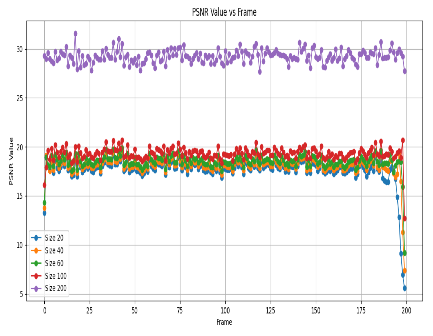
Figure 2.
RSE Comparison across Different Sizes
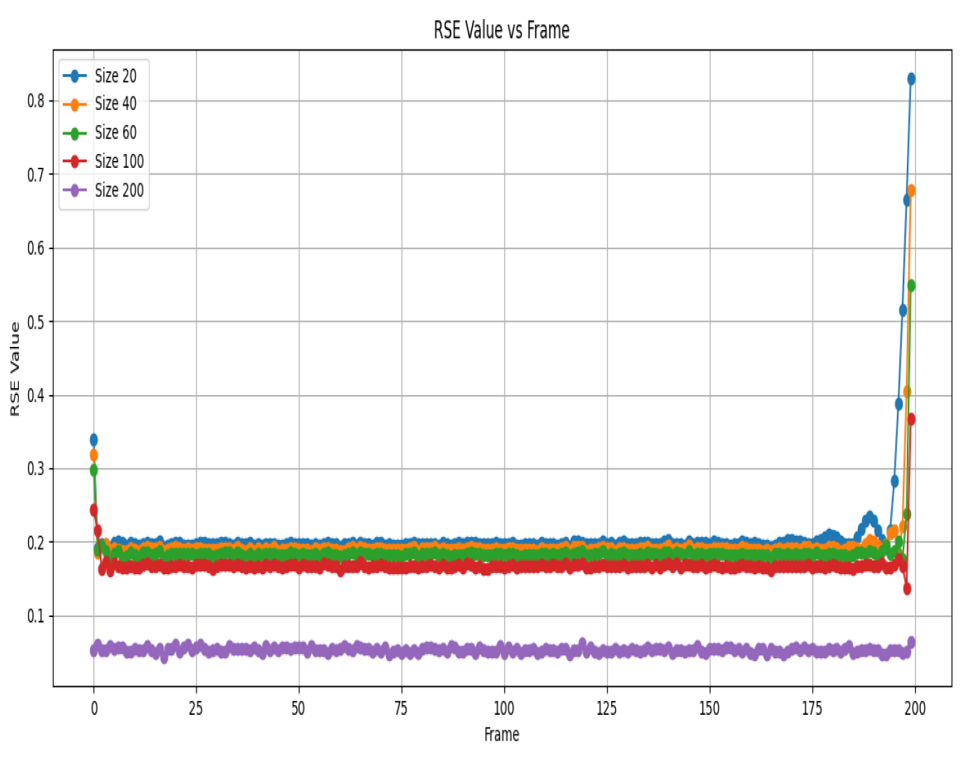
Figure 3.
PSNR Comparison across Different Sizess
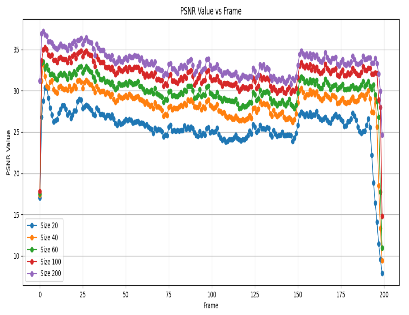
Figure 4.
RSE Comparison across Different Sizes
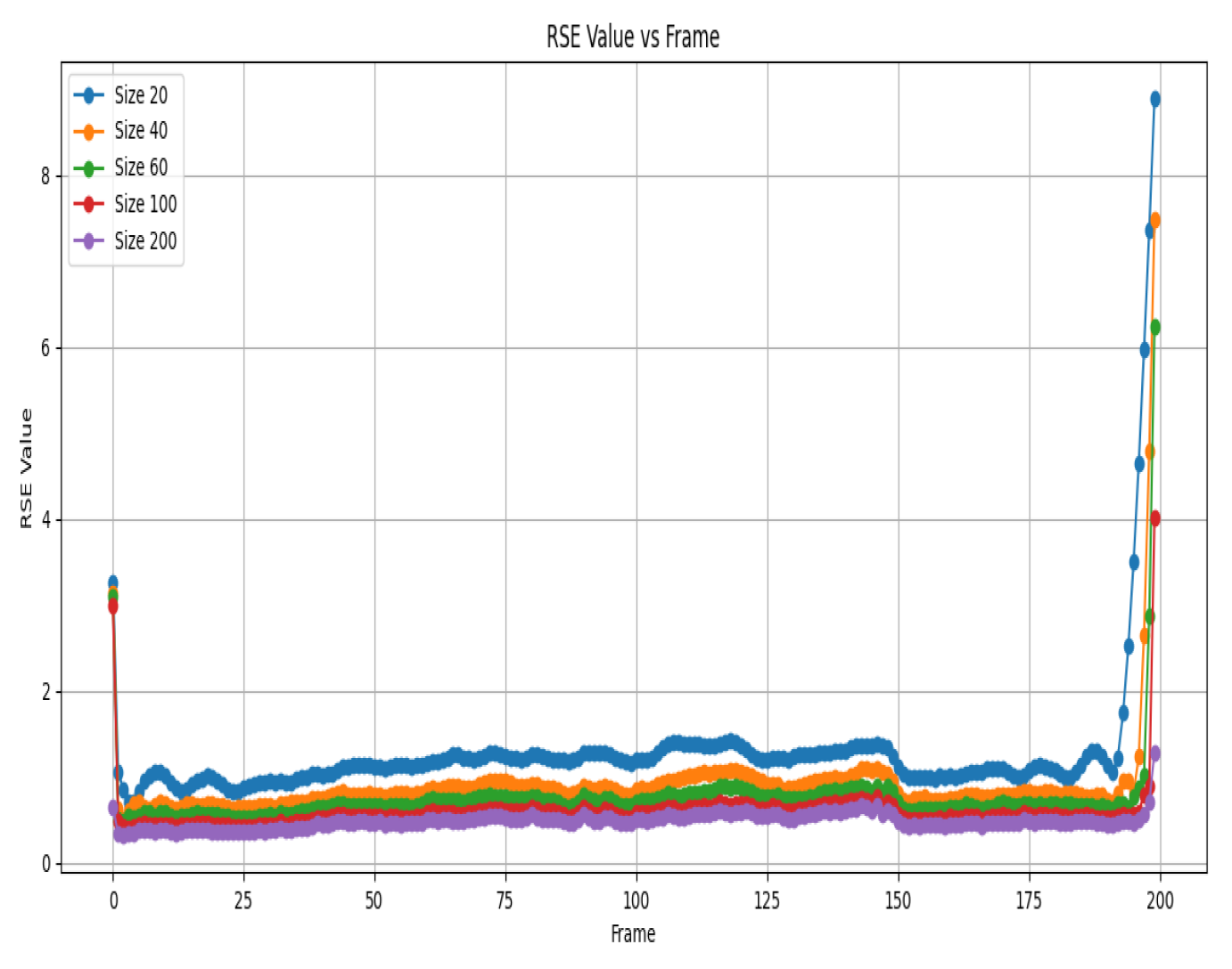
Figure 5.
Comparison of Denoised Images with TRPCA: Sizes = 20, 200(c-TRPCA) and frames=40,70,120
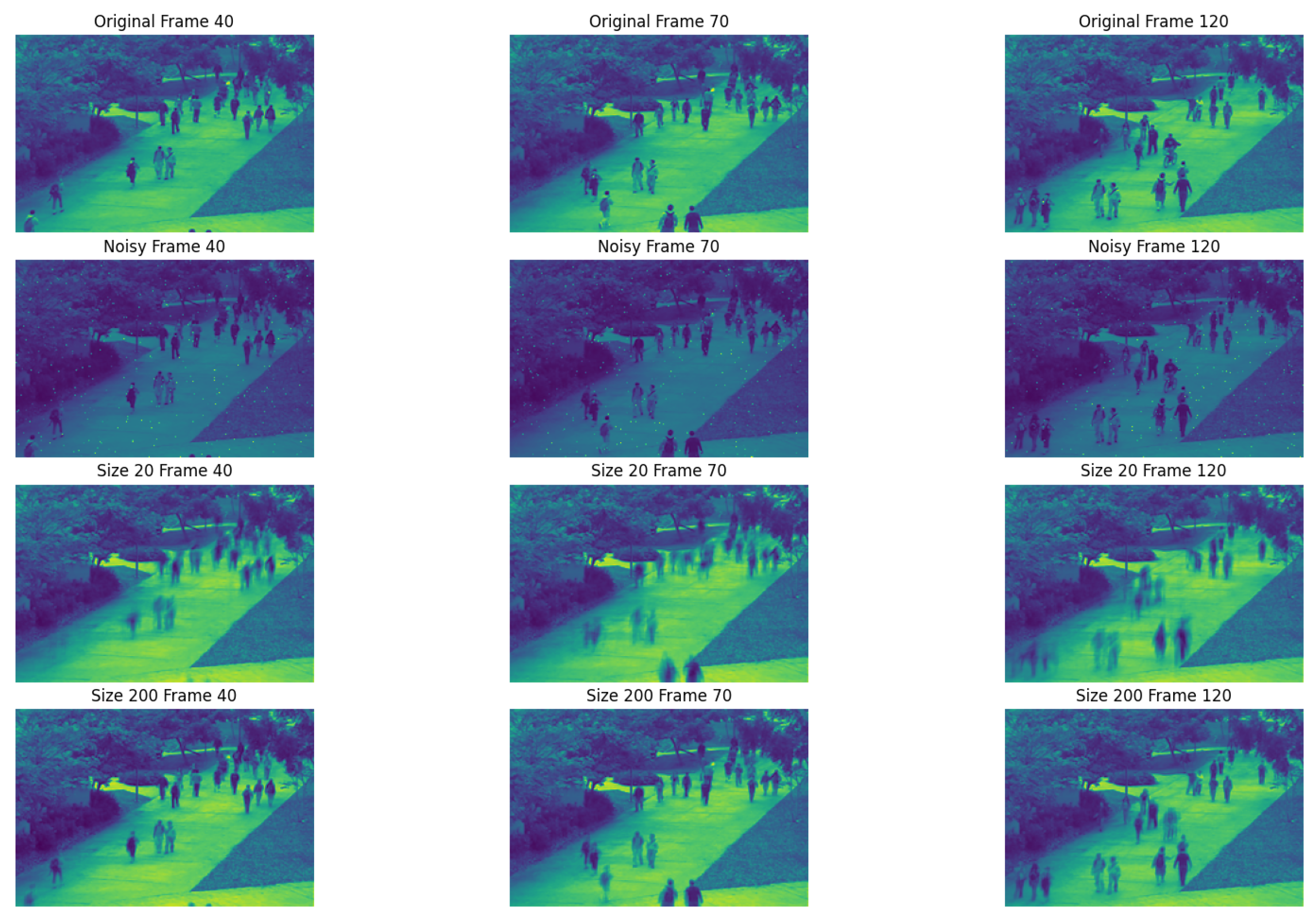
Figure 6.
Comparison of Residuals After Denoising with TRPCA: Sizes = 20,200(c-TRPCA) and frames=40,70,120
Figure 6.
Comparison of Residuals After Denoising with TRPCA: Sizes = 20,200(c-TRPCA) and frames=40,70,120
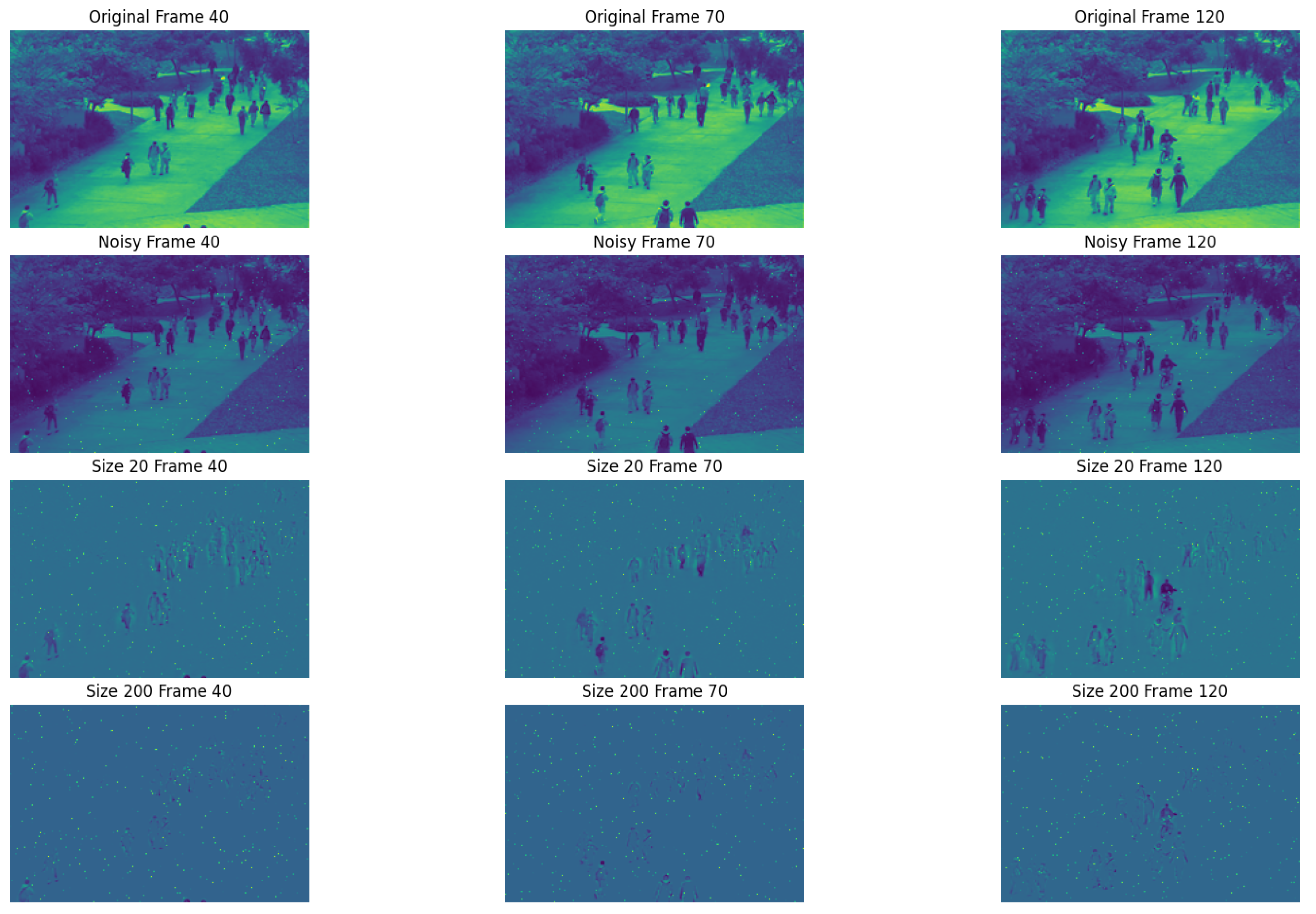

Table 1.
Ratio of Frobenius Norms for Different Sizes
| Size | 20 | 40 | 60 | 100 | 200(c-TRPCA) |
| Ratio | 0.9550 | 0.9639 | 0.9695 | 0.9788 | 1.0000 |
Table 2.
Comparison of runtime of different sizes
| Size | 20 | 40 | 60 | 100 | 200(c-TRPCA) |
| Run Time (seconds) | 128.2 | 150.9 | 258.8 | 314.2 | 694.7 |
Table 3.
Ratio of Frobenius Norms for Different Sizes
| Size | 20 | 40 | 60 | 100 | 200 |
| Ratio | 0.9824 | 0.9923 | 0.9957 | 0.9984 | 1.0000 |
Table 4.
Comparison of runtime of different sizes
| Size | 20 | 40 | 60 | 100 | 200 (c-product) |
| Run Time (seconds) | 402.63 | 550.03 | 664.75 | 1254.44 | 2026.47 |
Disclaimer/Publisher’s Note: The statements, opinions and data contained in all publications are solely those of the individual author(s) and contributor(s) and not of MDPI and/or the editor(s). MDPI and/or the editor(s) disclaim responsibility for any injury to people or property resulting from any ideas, methods, instructions or products referred to in the content. |
© 2024 by the authors. Licensee MDPI, Basel, Switzerland. This article is an open access article distributed under the terms and conditions of the Creative Commons Attribution (CC BY) license (http://creativecommons.org/licenses/by/4.0/).
Copyright: This open access article is published under a Creative Commons CC BY 4.0 license, which permit the free download, distribution, and reuse, provided that the author and preprint are cited in any reuse.


