
Submitted:
28 February 2025
Posted:
03 March 2025
You are already at the latest version
Abstract
Solid waste treatment and resourceization critically depend on waste characterization. Heavy metals and critical raw materials are found as trace elements in solid waste dumps. Their reliable quantification plays a critical role for decision risk regarding effective waste management. Reliable quantification of trace elements is a very difficult issue. Hence, the paper addresses a new conservative approach for data analysis in screening for trace element in waste dumps. We propose a theoretical model for statistical data interpretation to overcome the drawbacks of the conventional approaches that are based on unproved hypotheses, like binomial, Poisson or Gaussian distributions of the particles carrying the analyte. Our model addresses concentration values close to the limit of quantification (LOQ) of an analytical method. The model fills the gap of data analysis in case where a set of laboratory outcomes are uniform distributed. Our approach cope with results reported as lower than LOQ. The model was applied on XRFS results carried on tailings to emphasize the differences among classic, robust and conservative data analyses. Classical analyses overestimate the concentration values and sub-evaluate the associated uncertainties which enhances the decision risk. The paper demonstrates that conservative approach is mandatory in case of screening for trace elements if concentration values are uniform distributed. The model can be applied to any solid waste dump, regardless the analytical method used for trace element screening.
Keywords:
secondary resource
; solid waste
; surveying
; trace elements
; critical raw materials
; heavy metals
; chemical analysis
; statistical data analysis
; uncertainty
; decision risk
1. Introduction
Secondary resources, mainly solid wastes, are important part of the Circular Economy, as they can substitute genuine resources and reduce the carbon foot print caused by genuine resource extraction [1] The recycling of solid waste streams would be ideally if the recyclers received clean streams of waste products, which would allow them to produce recovered materials of sufficiently high quality for reused in the same, or similar, products. (so-called closed loop recycling) [1]. However, many solid wastes contain significant amount of heavy metals (e.g., As, Ba, Cd, Cr, Pb, Hg, Se, etc.) [2,3,4].
The presence of heavy metals in a solid waste stream can limit it potential for recovery. For example, ferrous slag recycling in agriculture (e.g., soil fertilizer, soil amendment, soil pH improvement) or in road and pavement construction can create environmental issues if slag pollutes the soil through leaching toxic elements under raining waters action. [5,6]. Consequently, Resource Conservation and Recovery Act enforced by the Environmental Protection Agency stated allowable limits for heavy metals in soils [7]. Hence, reliable measurement of heavy metal contents in a solid waste stream is mandatory for mostly recovery applications.
Another significant challenge in waste management is the screening for critical raw materials (CRMs) in industrial solid waste dumps, as required by Regulation (EU) 2024/1252 [8]. Notably, this regulation mandates that:: “By 24 November 2027, Member States shall adopt and implement measures to promote the recovery of critical raw materials from extractive waste, in particular from closed extractive waste facilities”. Additionally, Regulation (EU) 2024/1252 (Article 27) obligates operators of extractive waste facilities in each EU Member State “to provide to the competent authority a preliminary economic assessment study regarding the potential recovery of critical raw materials, from waste stored in their facilities by 24 November 2026. The study shall at least include an estimation of the quantities and concentrations of critical raw materials contained in the extractive waste and in the extracted volume and an assessment of their technical and economic recoverability. Operators shall specify the methods used to estimate those quantities and concentrations.”
The transition of mineral waste from ‘waste’ to an asset for re-mining and recovery of CRMs requires representative sampling and appropriate data processing methods to assess its economic potential [9]. Tailings deposits are typically low-grade deposits of CRMs i.e., CRMs incidence in such waste is at trace level. Also, contaminants such as Pb, Hg, Cd are at trace levels in tailings. Thus, an accurate estimation of the CRMs and associated contaminants concentrations is crucial for safe recovery of the valuable minerals and for the implementation of zero-waste approach to enable proper reclamation of pond sites.
In case where, materials are regulated at low levels, as heavy metal contents, but not only, the analyst must establish whether the analytical method is capable of detecting the analyte at all at the regulated level [10]. Also, the officers that evaluate the conformity of the regulated analytes must differentiate between statements about an analytical result, which is known, and inferences about the true value, which is not known. It is also essential to understand that there are at least two quite different limits involved in analytical measurement i.e., limit of detection (LOD) and limit of quantification (LOQ) [10]. In conformity assessment based on upper limits, the challenge is the expanded uncertainty associated with a low-level concentration value [11]. The issue of reliable assessing of the targeted analyte in case it belongs to CRMs list is complicated by the fact that the CRMs concentrations in earth crust are of the parts-per-million (ppm) range [12,13,14]. According to F. Pittard, ”There are no areas that are more vulnerable to such misfortune than sampling and assaying for trace amounts of constituents of interest in the environment, in high purity materials, in precious metals exploration, food chain, chemicals, and pharmaceutical products” [15]. Therefore, a correct evaluation of the concentration value of the targeted analyte at lot scale and of its uncertainty has two benefits i.e., 1) support triggering the investment for CRMs harvesting from a waste stream and 2) prevent the decision risk in mining for precursors of the CRMs or precious metals. Additionally, a conservative approach applied in conformity assessment can mitigate the erroneous decision regarding false positive and false negative when contents of the trace elements are tested [16].
The statistical data analysis in sampling of the grained/particulate solid wastes for trace constituents is often based on mass/discrete probability distributions like Poisson distribution, double Poisson distribution or binomial distribution [15,17,18,19,20,21,22]. In the frame of discrete distributions, a granular waste lot is conceptually modelled as a population of particles, each one having or not the targeted property like a chemical concentration, a nugget mineral or a generic property. In this context, sampling from a population of discrete material (e.g., a solid waste lot) is a random selection of a subset (i.e., a “sample”). The sample/subset is representative if it contains a reliably similar proportion between particles of interest and the particles occurring in the batch of materials to be characterized. In the case of tailings and other fine-grained substances, this approach has at least three drawbacks:
i) the concentration of an analyte in a waste particle is rather a continuous function. This contradicts the hypothesis of analyte distribution in a constant quantity in some particles while others contain zero analyte. Accordingly, the discrete distributions are unsuitable for statistical data interpreting in case of fine-grained solid wastes;
ii) an analyte can exist in different particles as part of dissimilar compounds. This contradicts the assumption that a particle contains a constant quantity of analyte, further rendering discrete probability models inappropriate.
iii) the discrete sampling (particle by particle) is inappropriate in case of fine-grained wastes like tailings, bottom ashes etc. Instead, incremental sampling is the standard approach in sampling of the fine-grained waste dumps [14].
Analytical procedure applied to trace elements require sample comminution i.e. crushing, milling and, sometimes, analyte extraction through chemical or physical methods [14,23,24]. A well-prepared sample results in a homogenized analyte distribution, meaning that analytical results reflect the mean concentration of the aliquot. However, even with homogenization, the dependence of analytical results on aliquot size cannot be eliminated..
Our proposed approach aims eliminate the unproven hypothesis of the granularity of the analyte (nudged distribution) contained in the targeted lot, which is often adopted in existing literature without supporting evidences [15,18,19,20]. To overcome the limitations of conventional approaches, we present a new theoretical model designed to enhance data interpretation for incremental sampling of fine-grained substances, including tailings, pharmaceutical powders, food etc. [24].
The key concept of the model is assigning of a uniform probability density function (pdf) to the analyte mass in aliquot and a triangular pdf to the aliquot mass. The rationale for assigning a uniform pdf to the mass of the targeted analyte is based on the evidence that a 1 g of fine-grained sub-sample may contain over a million particles of some mixed minerals. Also, an analyte may exist both as grains or in atomic state incorporated in different minerals. ISO 98-3 recommends using a uniform pdf when little information is available about an assessed quantity [25]. These considerations support attributing a uniform random variable to the targeted analyte mass .
It is worth noting that the concentration of the analyte, its uncertainty (standard or expanded) and the aliquot mass are the only data that a laboratory can provide for a sample that has undergone a chain of preparatory operations as to produce the analytical specimen, aka aliquot. Therefore, this data supports any decision regarding CRMs recovery from genuine and secondary resources.
Laboratory practice shows that the aliquot mass is weighed with high accuracy using a calibrated balance, whose uncertainty is certified. Usually, the calibration certificate of a balance does not specify the pdf of the assigned to the measurand. . When a calibration certificate specifies the volume of a flask as 1000 ± 5 mL, it is recommended to use a triangular distribution [26]. Therefore, triangular pdf is the best choice for the aliquot mass when it is considered as a random variable [25,26].
The theoretical model addresses both the ideal measurement case where analytical process does not introduce uncertainty and the practical one when analytical process distorts the results through unavoidable LOQ of the method and measurement uncertainty. The model emphasizes the critical role of mass reduction i.e., the primary sample mass of the order of kgs is reduced to aliquot mass of few grams. Accordingly, the weighing operation plays a critical role in the modeling of the probability distribution function ascribed to the concentration of a trace element.
The conservative approach for data analysis was applied in case of surveying iron ore tailings for CRMs through incremental sampling. The concentrations of major, minor and trace elements of the collected samples were measured by energy dispersive X-ray fluorescence spectrometry (ED-XRFS). Handheld and benchtop ED-XRFS techniques are frequently used for surveying purposes as they are fast, accessible and reliable for elemental analysis [14,27,28]. There are some other X-ray based techniques that can be used for advanced studies of solid waste like X-ray absorption spectrometry, total reflection X-ray fluorescence spectrometry etc., that have the ability to measure trace levels of elements in the ppb range, to provide important information on local state of the atoms etc. [27,28]. It is beyond the scope of this paper to discuss the advantages offered by recent developments of these techniques. The reader interested in the application of advanced X-ray based techniques may find valuable information in dedicated literature like [27,28].
The way of raw data processing for each X-ray base technique is a matter of intellectuals property of the producer. The statistical analysis of a suite of results provided by an X-ray technique in a laboratory is performed based on classical statistical approach [26]. The data analysis in the proficiency testing scheme is done both on classical and robust statistics [29].
This study contributes novel insights to the statistical analysis in the data analysis when surveying for trace elements, including CRMs, by addressing entire process of data acquisition i.e. sampling, sub-sampling and laboratory analysis. Furthermore, it introduces the novel idea of disregarded the analyte concentration from its carriers i.e. analytes can be found as atoms in compounds, as nugget whatever. Thus, this approach avoids using discrete distributions of the particles that carries targeted analyte, that is unfitted for purpose of data interpreting in screening for trace elements.
The superiority of the proposed conservative approach over classical and robust statistical data analyses is demonstrated in cases where it is found a uniform data distribution nearby detection limit. Additionally, the decision risk associated with solid waste recycling is highlighted, particularly when traditional statistical analyses lead to overestimated analyte concentrations and underestimated uncertainties. The approach we advance can facilitate a dipper insight view on analyte distribution in targeted batch (lot, stockpile) through statistical modelling of the entire measurement chain i.e., sampling and analytical measurement. The model is versatile i.e., it can be applied to any incremental sampled fine-grained substance in case where the distribution of the analyte in the lot is unknown.
2. Materials and Methods
This paper is largely theoretical; therefore, the first part of this section is dedicated to deriving the statistical background of the proposed conservative approach. The latter part discusses the SEM-EDS and XRFS investigations, which provide the data necessary to demonstrate the applicability of the conservative approach.
2.1. Derivation of the pdf Assigned to True Analyte Concentration into the Aliquot
The mass concentration of an analyte in a sub-sample is considered a random continuous variable (R), defined as the ratio of analyte mass (Y) to the aliquot mass (X). Both X and Y masses are considered random continuous variables. According to standard laboratory procedures, an aliquot is taken from a comminuted sample and carefully weighed for an intended analytical measurement. The laboratory practice under ISO EN 17025 standard imposed high exactness for the aliquot mass measurement [30]. The uncertainty of a laboratory weighing is less than 10-2 g for the masses of several grams. In such a case, a triangular probability density function (pdf) can be assigned to the X mass [26].
where m is the mean mass of the aliquot and a is the largest weighing error.
The analyte mass Y is considered a random variable whose value in a sample of X mass is unknown and very difficult to establish through experimental trials. The ISO 98-3 standard [25] recommends assigning a uniform pdf in case where no reliable information exists about a random variable. In this respect, a uniform pdf is assigned to the analyte mass Y contained in an aliquot.
where b is the maximum mass of the analyte in an aliquot.
2.2. Derivation of the pdf Assigned to True Analyte Concentration into the Aliquot
The analyte concentration into aliquot is the ratio R= Y/X. The cumulative distribution of R is [31]:
where fX(x) and fY(y) are the pdfs assigned to the variables X and Y, respectively.
The upper limit of integration in Eq. (4) depends on r value as it is shown in Figure 1 i.e., for r < b/(m+a), u belongs to the interval [m-a; m+a]. In case where rranges from b/(m+a) to b/(m-a), (green line in Figure 1), the upper limit of integration is b/r. Therefore, is a branched function defined on the intervals: [0; b/(m+a)], [b/(m+a); b/m] and [b/m; b/(m-a)].
The value of the R variable assigned to analyte concentration in a specimen ranges from 0 to b/(m-a). The range [0, b/(m-a)] is divided in 3 intervals [0; b/(m+a)], [b/(m+a); b/m] and [b/m; b/(m-a)] because the different ways of superposing between uniform distribution and the triangular distribution. In the range [0; b/(m+a)], R intersects entire distribution of X, while in the intervals [b/(m+a); b/m] and [b/m; b/(m-a)], R intersects only a part of the triangular distribution of X as is shown in Eqs. 5-7.
In case where r [0; b/(m+a)], the is calculated as:
Eq. (5) shows that R is uniform distributed for r [0; b/(m+a)].
In case where r [b/(m+a); b/m], the second branch of the pdf of R, denoted is calculated as:
respectively
In case where r [b/m; b/(m-a)], the third branch of the pdf of R, denoted is calculated as:
The true analyte concentration is calculated as the mean of R, denoted by i.e.
The mathematical expression of the expectance of R is:
where ln() is the natural logarithm.
Considering that a/m ≤ 10-2, then the expression of in Eq. (10) can be better perceived if its expression is expanded in Maclaurin series depending on z = a/m variable, respectively
The expression of the mean value of the analyte concentration in Eq. (11) is similar to that of a uniform distribution i.e., b/(2m) except a tiny increasing which is at least less than 1.7*10-5 %, depending mainly on weighing uncertainty.
The variance of the analyte concentration, denoted by σ2, is calculated as
where
The mathematical expression of the variance of the R variable is:
Based on the same argument as in case of Eq. (10), we used the Maclaurin series expansion of Eq. (14) to get a more significant form of i.e.,
The variance of R is close to the variance in case where it is uniform distributed, but it contains a supplementary positive term which increases its value. The increasing rate is i.e., in practice, less than 0.05%.
In case where z ≤ 10-2, the coefficient of variation (CV) of R is:
The CV value of R is specific to a uniform pdf in case where the weighing error is less than 10-2 g. Otherwise, CV will be a function of z = a/m, whose derivative is positive i.e. CV(z) is minimum for z = 0 and increases as z increases.
The model described above can be applied in the case of an ideal concentration measurement where the laboratory provides an exact concentration values in the range [0, b/(m-a)]. Laboratory practice shows that any analytical procedure is characterized by a limit of detection (LOD), LOQ, an analytical range and uncertainty of the result estimated as standard deviation (SD) or expanded uncertainty [10,32,33]. Therefore, the results provided by an analytical method will be altered to some extent. Therefore, further considerations are necessary to estimate the effects of the laboratory analysis on the resulting values.
2.3. Derivation of the Analyte Concentration with Laboratory Constrains
When the concentration of a sample is measured using an instrumental or wet chemical procedure, the measured value will differ from the true concentration R due to analytical errors and other uncontrollable factors. To account for measurement uncertainty, one has to introduce a random variable (error variable) E, provided that its pdf is known. In case of instrumental analysis (e.g., XRFS, ICP etc.) E is typical considered to be normally distributed due to many influence factors that contribute to the measurement uncertainty budget. According to the Central Limit Theorem when the number of influence factors exceeds 30, then the convolution of their pdfs results in a normal pdf [31]. A measurement procedure cannot tolerate large errors; therefore, a truncated normal pdf must be assigned to E, denoted fE(e) [34] i.e.
where ε is the largest error and KE is the normalized constant i.e.
where Φ() is the cumulative distribution function of the standard normal distribution N(0;1)
The variable assigned to the concentration provided by a laboratory that has a LOQ=0 is:
C=R+E
Assuming that the parameters of the pdf of E are known i.e. σE and ε, then the calculation of the mathematical expression of fC(c) can be done based on convolution method [32]:
where is the convolution operator.
As the is the convolution of fR (r) and fE(e) functions, then its characteristic function CC(t) is the product of the characteristic functions assigned to the pdfs of the variables R and E, respectively [36]. The characteristic functions of variable R, denoted is defined as:
The is defined in the same way.
According to convolution theorem the characteristic functions of C variable is:
Based on the mean of C, denoted , the square mean of C, denoted , were calculated as follows:
The variance of C is:
As could be observed in Eq. (25), a measurement process that introduce errors having a truncated normal distribution do not affect the mean value of the true concentration (R) but increases the variance of the true concentration (.
The measurement process imposes a constraint on the analytical domain [q, Q], where q is the minimum measurable value and Q is the maximum measurable value of the specific procedure. In practice, q can be considered equivalent to LOQ. Consequently, R values ranging from 0 to LOQ cannot be reported for a given analytical method. When an analyte concentration cannot be quantified with a certain confidence level it is reported as less than a q value which is frequently improper named as “lower limit of detection” [33]. Hence, the measurement procedure implies the truncation of the i.e., the left side of the distribution is removed in the interval [0, q]. The pdf of the truncated Cvariable, denoted g(c), is:
The truncation caused by analytical procedure will alter the mean concentration and variance calculated based on analytical data. As an example, in case where is supposed to be uniform in the range [0, b/m] then the expectation of g(c), is:
Eq. (27) shows that the mean value of a trace concentration (some ppm) obtained based on measurement results is greater than its true value with 0.5*q, which is 0.5*LOQ. If LOQ is 4 ppm and averaged value is 6 ppm than the true value of the mean is 4 ppm i.e. the relative error is 50%.
The variance of g(c), denoted s2, decreases
The decreasing of variance of g is caused by cancelation of the very low values of C equivalent with shortening the spreading range of C.
Notwithstanding that the truncation of C values introduces an additional risk in risk on decision making regarding CRM recovering, as it creates a positive confidence by false increasing of the concentration mean and decreasing its uncertainty.
An exact mathematical treatment of the truncation effects caused by the LOQ of the analytical method using the above derived expression is beyond the scope of this paper. However, an approach is proposed to overcome this drawback. Supposing a set of N specimens is measured under reproducible conditions in a qualified laboratory and the maximum value, cmax, is obtained. The range [0, cmax] can be divided into n intervals, n = [cmax/q]+1, where [cmax/q] is the integer part ofcmax/q. Subsequently, a histogram of the results should be constructed using n bins, each with a width of q. Data reported as lower than “limit of detection” are assigned to the first bin. If a statistical test confirms that the data are uniform distributed, then the concentration of the targeted analyte is uniform distributed in measured specimens. Therefore, the model posted in this paper can be applied for conservative data analysis i.e., the true mean and its standard deviation should be considered as:
In case where the histogram shows data clustering then another distribution of the analyte should be identified.
2.4. Sample preparation and characterization
The old and abandoned Teliuc tailings pond in Romania, was explored aiming the screening the presence of certain CRMs (Figure 2). It is located at 45°44′08″N 22°53′01″E coordinates and has an area of approximately 35 ha. Teliuc pond contains approximately 5.0*106 m3 waste resulting from iron ore processing through flotation. A large area of the Teliuc pond surface (Figure 2) is still not covered by vegetation. However, this pond still pollutes the surrounding area, at least with flying dust. Additionally, it can pollute the soil and underground water through heavy metals leached by the raining water. The screening for CRMs in tailings was suggested by literature reports [37,38]. There were collected 40 samples across the surface of the dump. The full characterization of the tailings is beyond the scope of this paper, as we address only an example of how to apply the data analysis model posted in this paper regarding the CRMs content in the pond.
The collected gross sample of tailings weighed approximately 4 kg. The gross sample was crushed, grinded, and milled until achieving a powdered state using home made laboratory crushers and grinding mills. The fraction that had been sieved using a 1 mm mesh was coned, then quartered, and a subsample weighing about 0.5 kg underwent advanced milling using a ball mill (Retsch GmbH, Haan, Germany). The milling process lasted until the residue on the sieve (65 μm mesh) was less than 10%. The powder that passed through a 65 μm mesh sieve underwent subsampling through coning and quartering, and circa 50 g of the powder was selected for XRFS measurements. Scanning Electron Microscopy with Energy Dispersive Spectroscopy (SEM-EDS) was used to evaluate the tailings heterogeneity, in terms of both mineralogy and elemental composition. This information is essential for a deeper understanding of the waste condition and to establish the methods for its adequate characterization. The SEM-EDS observations were performed with a Zeiss EVO 50 XVP (Carl Zeiss NTS , Jena, Germany) equipped with LaB6 electron gun and an EDS accessory from Bruker. The oxide and elemental concentration were measured through a Xepos ED(P)-XRF spectrometer (SPECTRO Analytical GmbH, Kleve, Germany)). The decision to use ED-XRFS technique was based on its figure of merit i.e., cost efficiency ratio. XRFS allow for simple, rapid and cheaper sample preparation while ICP-MS, ICP-AAS, AAS etc., need a complicated sample preparation process-like sample dissolution or digestion that may introduce a number of additional chemicals [36,37].
The aliquots for XRFS measurements were prepared as Pressed Pellet. The pellet contains 7.25 g of tailings. The XRF spectra were processed with the TurboQuant Pellets analytical program.
3. Results and Discussion
3.1. Assessment of the Tailings Heterogeneity at Micro-Scale
The particle size and morphology in tailings body vary in unpredictable ways as Figure 4 shows.
SEM images reveal aggregated particles that look like being amorphous (Figure 4a, b, c). Figure 4d shows the presence of particles with crystalline shapes. Point-specific EDS analysis performed on the tailings depicted in Figure 4 indicates chemical heterogeneity at micro-scale. (Figure 5).
The EDS analysis in Figure 5. a, shows concentration values that are significantly different from those in Figure 5. B. Notably U is measured in the second specimen (Figure 5. b), while in the first one (Figure 5. a) it is undetected. These findings from the SEM and EDS investigations support the hypothesis of assigning uniform distribution to the quantities of trace elements in the tailings aliquots.
The XRFS measurements yield results that must be interpreted as mean values at a scale of approximately one Kg, as the collected sample is homogenized prior to sub-sampling the aliquot used for testing. The XRFS results include both major and minor components of the tailings, as presented in Table 1, which lists the results for aliquots no.1 and no. 22 are posted. The aliquots no. 1 and no. 22 were randomly chosen to emphasize that there is no bias regarding XRFS analyses.
The analytical range of Xepos instrument covers many of the CRMs (V, Ga, Ge, Rb, Y, Nb, Mo, Ag, Cd, Sb, Te, La, Ce, Hf, Cs, Bi) as well as heavy metals (As, Cd, Cr, Hg, Pb Se). XRFS results indicate that these elements are at trace level in these tailings. (Table 1).
Given that the analysis of CRMs in tailings using XRFS is of greater current interest than that of heavy metals, the application of the developed model for statistical data analysis is focused on selected CRMs. For instance, the concentrations of La, Te, Hf are below their respective LOQ values, while those of Ga, Y, Sr exceed their respective LOQs. Bi and Ge serve as examples of CRMs whose concentrations fluctuate below and above their LOQ values. To better illustrate data analysis, Y, Ce, Ge and Bi were selected. Their measured concentration values in 40 specimens along with their associated standard uncertainties, are presented in Table 2.
The histograms of Y and Ce (Figure 6) show that their concentration values have a clustering tendency. The absolute frequency values posted on each bin in Figure 6 a, b, indicate that left side tails of the histograms are heavier than the right ones. This demonstrates that the empirical distributions of Y and Ce concentration values are burden with smaller values due to the prevalence of the aliquots with lower content of Y and Ce. The theoretical distribution that can be assigned to the empirical distributions in Figure 6 can be assumed as normal, but applying statistical inference to demonstrate the adequacy of normal distribution for the data in Figure 6 is beyond the scope of this paper. According to Central Limit Theorem, the arithmetic means of the Y and Ce concentrations follow normal distributions N(21.5, 0.3) and N(34.6, 1.2), respectively.
Robust statistical analysis conducted in accordance with ISO 13508 [29] and ISO 5725-5 [38] provided closer value for Y (median 21.4, with a standard deviation of 1.3) while for Ce the median is 34.5 ppm with a standard deviation of 1.8 ppm. The model we advance above is not applicable for Y and Ce elemental concentration, as their concentration values are all above the LOQs and exhibit a clustering tendency. However, for Ge and Bi the use of the proposed model is mandatory as some of their concentration values fall below their LOQs and the histograms of the data suggest a uniform distribution of the analytical outcomes (Figure 7).
The histogram of the concentration values for Ge and Bi do not exhibit a clustering tendency and suggest that the concentration values are uniform distributed (Figure 7 a, b). Clearly, a larger set of data would better underpin the hypothesis of their uniform distribution, but it would entail a higher cost and significantly more laboratory work.
An investment decision in mining for precursors of the CRMs and of the precious metal is mainly based on averaged values of the targeted analyte at lot scale and on the uncertainty assigned to this value. The averaged value and its assigned uncertainties depend on the statistical approach applied to averaged data as is shown in the paper. The comparative data analyses through classical, robust and comprehensive approaches (Table 3) aims demonstrating that in case of uniform distributed entry data, the approach posted in the paper yields the most reliable values of the concentration mean and its assigned uncertainty. To highlight the differences among the classical and robust statistical analyses of the data and the approach proposed in the paper, we performed classical and robust analysis of the data in Table 2. The classical statistical analysis of the data in Table 2 relies on arithmetic mean, the standard deviation (SD) and relative SD, denoted RSD, which is akin to the coefficient of variation. The data analysis according to our approach takes into account a=0.01 g, m=7.25 g, and analytical uncertainty equal to the LOQ specified by the TurboQuant analytical software as it is specified in Table 3.
4. Discussion
The XRFS reported a LOQ = 0.5 ppm for Ge and a LOQ = 1.0 ppm for Bi. 5 outcomes were reported as below the LOQ for Ge and 6 for Bi. Robust statistical analysis of the data for Ge yielded a median of 2.2 ppm and a standard deviation of 1.9 ppm, while for Bi a median of 3.2 ppm with a standard deviation of 1.9 ppm.
Applying the conservative model proposed in this study, the mean concentration of Ge is calculated as 2.9 ppm which is higher than that provided by the robust statistical analysis with approximately 0.7 ppm i.e. with approximative 32% greater. For Bi, the conservative approach yields a mean concentration value of 3.3 ppm, which is very close to the robust estimation value of 3.2 ppm representing an increase of approximative 3% greater. The conservative approach reveals higher standard uncertainties in these cases - approximately 3.4 ppm for Ge and circa 3.9 ppm for Bi, that exceed the concentration values themselves. In such cases, the data are deemed unreliable for decision-making regarding the recovery of Ge and Bi.
The data analysis model we proposed herein produced contradictory results for Y and Ce (Table 3), due to their concentration exhibiting a clustering tendency (Figure 5. a, b). This outcome aligns with the limitations of our model as it is valid only for uniformly distributed data, such as in the cases of Ge and Bi (Figure 6 a, b).
The classical statistical analysis overestimates the Ge and Bi concentration values with circa 59% and 15%, respectively. Similarly, robust statistical analysis overestimates the Ge and Bi concentration values with circa 43% and 7%, respectively. Additionally, the SDs assigned to the concentration values using the classical and robust data analysis are underestimated(Table 3). This evidence demonstrates that both classical and robust statistical analyses of the concentration values close to the LOQ of a suite of results that are uniform distributed yield higher values than real (true) ones. Such data analyses may lead to a false positive decision regarding investment in a trace element recovery business. Therefore, when there is evidence that analytical outcomes are uniform distributed, it is prudent to apply a statistical analysis based on the conservative approach outlined earlier in this paper.
5. Conclusions
The conservative approach is designed for data analysis when surveying for trace elements in fine-grained waste deposits, such as CRMs and heavy metals. The discrete distributions are inoperant in such cases. Given that that even-grained solid wastes are comminuted and milled before chemical and mineralogical analyses, it is evident that discrete distributions are inoperant for statistical data analysis in screening of solid waste.
The proposed model is designed to cover the gap of statistical data analysis as fundamental theoretical approach, particularly in cases where the outcomes indicate a uniform distribution of the targeted elemental concentration values.
The theoretical framework encompasses both the ideal and practical measurements scenarios. In an ideal measurement case, the analytical process does not introduce uncertainty, while in practical situations, the analytical process distorts the results due to unavoidable LOQ of the method and measurement uncertainty.
A key finding of the paper is the effect of the weighing on the derivation of the concentration pdf. The weighing exactness allows the assignment of a triangular pdf to the aliquot mass variable X with a very narrow CV, which effectively behaves as a Dirac distribution relative to the pdf of the analyte mass variable, X.
The conservative approach was applied to a survey of iron ore tailings for CRMs, using incremental sampling followed by XRFS analyses. This application aims to demonstrate the advantages of the conservative approach compared to classical and robust statistical analyses. It was found that classical and robust statistical analyses of the concentration values close to the LOQ, for a suite of results that are uniform distributed, yield higher values and smaller uncertainties. Consequently, classical statistical data analysis may present a false positive picture of a solid waste pile’s contents, potentially leading to an erroneous decision to invest in a trace element recovery.
The relative uncertainty in measurement reflect better the precision of the entire analytical chain, including statistical data processing. As the its value is smaller as the measurement prosses woks better. Additionally, the relative uncertainties allow comparing measuremet procedures in cases where they are correct asessed. The data posted in Table 3 highligth situations when diffrent statistical data processing yield diffrent relative uncertainties values. The proposed approach is deemed as the most reliable among classical, robust and comprehensive data analyses in case where data are uniform distributed.
The approach we propose offers dipper insight into analyte distribution within a targeted batch (e.g., lot, pile, pond, dump) through statistical modelling of the entire measurement chain, encompassing both sampling and analytical measurement. The model is versatile and can be applied to any fine-grained substance that is incrementally sampled when the distribution of the analyte in the lot is unknown.
Author Contributions
Conceptualization, A.L.T, I.P., A.P. and C.U.; methodology, A.L.T., I.P, A.P. Z.K. and D.F.M; software, A.P., R.-N.T. and G.I.; validation, I.P., C.U. F.N and A.C.M.; formal analysis, Z.K, R.N.T and D.F.M; investigation, A.L.T., I.P, C.U., F.N, G.I. and A.C.M.; resources, A.L.T., A.P., Z.K., G.I. D.F.M and A.C.M.; data curation, C.U., F.N., G.I. and A.C.M.; writing—original draft preparation, I. P., C.U., R.N.T. and G.I.; writing—review and editing, I. P., A.P., R.N.T. and G.I.; visualization, I.P., Z.K., F.N., R.N.T. and G.I.; supervision, A.L.T., I.P.; project administration, A.-L.T. and A.P.; funding acquisition, A.L.T., A.P., C.U., ZK. And D.F.M. All authors have read and agreed to the published version of the manuscript.
Funding
This research received no external funding.
Institutional Review Board Statement
Not applicable.
Informed Consent Statement
Not applicable.
Data Availability Statement
Data available on request.
Conflicts of Interest
The authors declare no conflict of interest.
References
- GACERE (2024). Circular Economy and Solid Waste - Working Paper. Available online: https://www.unido.org/sites/default/files/unido-publications/2024-06/orking%20Paper_Circular%20Economy%20and%20Solid%20Waste.pdf (accessed on 20 January 2024).
- European Commission DG ENV. E3 Project ENV.E.3/ETU/2000/0058 Heavy Metals in Waste Final Report February 2002, file:///D:/2025/heavy_metalsreport.pdf.
- Document number C(2009) 3013), (2009/360/EC), COMMISSION DECISION, 30 April 2009, completing the technical requirements for waste characterisation laid down by Directive 2006/21/EC of the European Parliament and of the Council on the management of waste from extractive industries. Available online: https://eur-lex.europa.eu/egal-content/EN/TXT/?uri=CELEX:32009D0360.
- Onwualu-John, J.N.; Uzoegbu, M.U. Physicochemical Characteristics and Heavy Metals Level in Groundwater and Leachate around Solid Waste Dumpsite at Mbodo, Rivers State Nigeria. J. Appl. Sci. Environ. Manag. 2022, 26, 2107–2112. [Google Scholar] [CrossRef]
- Simon, F.G.; Scholz, P. Assessment of the Long-Term Leaching Behavior of Incineration Bottom Ash: A Study of Two Waste Incinerators in Germany. Appl. Sci. 2023, 13, 13228. [Google Scholar] [CrossRef]
- Das, S.; Galgo, S.J.; Aam, M.A.; Lee, J.G.; Hwang, H.Y.; Lee, C.H.; Kim, P.J. Recycling of ferrous slag in agriculture: Potentials and challenges. Crit. Rev. Environ. Sci. Technol. 2020, 52, 1–35. [Google Scholar] [CrossRef]
- United States Department of Agriculture Natural Resources Conservation Service Soil Quality Institute 411 S. Donahue Dr. Auburn, AL 36832 334-844-4741 X-177 Urban Technical Note No. 3 September, 2000. Available online: https://semspub.epa.gov/work/03/2227185.pdf.
- REGULATION (EU) 2024/1252 OF THE EUROPEAN PARLIAMENT AND OF THE COUNCIL of 11 April 2024 establishing a framework for ensuring a secure and sustainable supply of critical raw materials and amending Regulations (EU) No 168/2013, (EU) 2018/858, (EU) 2018/1724 and (EU) 2019/1020. Available online: https://eur-lex.europa.eu/eli/reg/2024/1252/oj (accessed on 8 July 2024).
- Dino, G.A.; Rossetti, P.; Perotti, L.; Alberto, W.; Sarkka, H.; Coulon, F.; Wagland, S.; Griffiths, Z.; Rodeghiero, F. Landfill mining from extractive waste facilities: The importance of a correct site characterisation and evaluation of the potentialities. A case study from Italy. Resour. Policy 2018, 59, 50–61. [Google Scholar] [CrossRef]
- AMC Technical Brief, The edge of reason: Reporting and inference near the detection limit Analytical Methods Committee AMCTB No. 92. https://doi.org/10.1039/C9AY90188D. Anal. Methods 2020, 12, 401–403. [CrossRef]
- Thompson, M.; Ellison, S.L.R. Towards an uncertainty paradigm of detection capability. Anal. Methods 2013, 5, 5857–5861. [Google Scholar] [CrossRef]
- Wikipedia, Abundance of elements in Earth's crust. Available online: https://en.wikipedia.org/wiki/Abundance_of_elements_in_Earth%27s_crust (accessed on 30 March 2024).
- Baldassarre, G.; Fiorucci, A.; Marini, P. Recovery of Critical Raw Materials from Abandoned Mine Wastes: Some Potential Case Studies in Northwest Italy. Mater. Proc. 2023, 15, 77. [Google Scholar] [CrossRef]
- Pencea, I.; Turcu, R.N.; Popescu-Arges, A.C.; Timis, A.L.; Priceputu, A.; Ungureanu, C.; Matei, E.; Nedelcu, L.; Petrescu, M.I.; Niculescu, F. An improved balanced replicated sampling design for preliminary screening of the tailings ponds aiming at zero-waste valorization. A Romanian case study. J. Environ. Manag. 2023, 331, 117260. [Google Scholar] [CrossRef] [PubMed]
- Pitard, F.F. Theoretical, practical, and economic difficulties in sampling for trace constituents. J. S. Afr. Inst. Min. Metall. 2010, 110, 313–321. [Google Scholar]
- Araya, N.; Ramirez, Y.; Kraslawski, A.; Cisternas, L.A. Feasibility of re-processing mine tailings to obtain critical raw materials using real options analysis. J. Environ. Manag. 2021, 284, 112060. [Google Scholar] [CrossRef] [PubMed]
- Sarker, S.K.; Haque, N.; Bhuiyan, M.; Bruckard, W.; Pramanik, B.K. Recovery of strategically important critical minerals from mine tailings. J. Environ. Chem. Eng. 2022, 10, 107622. [Google Scholar] [CrossRef]
- Pitard, F.R. Pierre Gy’s Sampling Theory and Sampling Practice: Heterogeneity, Sampling Correctness, and Statistical Process Control, 2nd ed.; CRC Press: Boca Raton, FL, USA, 1993. [Google Scholar]
- Minkkinen, P.O.; Esbensen, K.H. Sampling of particulate materials with significant spatial heterogeneity - Theoretical modification of grouping and segregation factors involved with correct sampling errors: Fundamental Sampling Error and Grouping and Segregation Error. Anal. Chim. Acta 2019, 1049, 47–64. [Google Scholar] [CrossRef] [PubMed]
- Hennebert, P. The sorting of waste for a circular economy: Sampling when (very) few particles have (very) high concentrations of contaminant or valuable element, 2019, 17th International waste management and landfill symposium, Santa Margherita di Pula (CA), Italy in Proceedings SARDINIA2019, 2019 CISA Publisher. Available online: www.cisapublisher.com.
- Hennebert, P.; Beggio, G. Sampling representative waste samples based on particles size. Detritus 2022, 18, 3–11. [Google Scholar]
- Hennebert, P.; Beggio, G. Sampling and sub-sampling of granular waste: Size of a representative sample in terms of number of particles. Detritus 2021, 17, 30–41. [Google Scholar] [CrossRef]
- Ladenberger, A.; Arvanitidis, N.; Jonsson, E.; Arvidsson, R.; Casanovas, S.; Lauri, L. Identification and quantification of secondary CRM resources in Europe, SCRREEN - Contract Number: 730227. Available online: https://scrreen.eu/wp-content/uploads/2018/03/SCRREEN-D3.2-Identification-and-quantification-of-secondary-CRM-resources-in-Europe.pdf (accessed on 19 February 2024).
- Gerlach, R.W.; Nocerino, J.M. Guidance for Obtaining Representative Laboratory Analytical Subsamples from Particulate Laboratory Samples. EPA/600/R-03/027 November 2003, ID: 75176. Available online: https://www.researchgate.net/publication/242671015_Guidance_for_Obtaining_Representative_Laboratory_Analytical_Subsamples_from_Particulate_Laboratory_Samples (accessed on 20 December 2024).
- ISO/IEC 98-3:2008; Uncertainty of measurement —Part 3: Guide to the expression of uncertainty in measurement (GUM:1995). ed. ISO: Geneva, Switzerland, 2008.
- Coskun, A.; Oosterhuis, W. Statistical distributions commonly used in measurement uncertainty in laboratory medicine. Biochem. Med. 2020, 30, 010101. [Google Scholar] [CrossRef] [PubMed]
- Terzano, R.; Denecke, M.; Falkenberg, G.; Miller, B.; Paterson, D.; Janssens, K. Recent advances in analysis of trace elements in environmental samples by X-ray based techniques (IUPAC Technical Report). Pure Appl. Chem. 2019, 91, 1029–1063. [Google Scholar] [CrossRef] [PubMed]
- Allegretta, I.; Bilo, F.; Marguí, E.; Pashkova, G.V.; Terzano, R. Development and Application of X-rays. Met. Anal. Soil Plants. Agron. 2023, 13, 114. [Google Scholar] [CrossRef]
- ISO 13528:2015; Statistical Methods for Use in Proficiency Testing by Interlaboratory Comparison. 2nd ed. ISO: Geneva, Switzerland, 2015; 10–12, 32–33,44–51, 52–62.
- ISO/IEC 17025:2017; General requirements for the competence of testing and calibration laboratories, ed. ISO: Geneva, Switzerland, 2017.
- Pencea, I. Multiconvolutional Approach to Treat the Main Probability Distribution Functions Used to Assess the Uncertainties of Metallurgical Tests, chapter 6 in Metallurgy - Advances in Materials and Processes. InTech, 2012; p. 186. ISBN 978-953-51-0736-1. [Google Scholar] [CrossRef]
- Kadachia, A.N.; Al-Eshaikhb, M.A. Limits of detection in XRF spectroscopy. X-Ray Spectrom. 2012, 41, 350–354. [Google Scholar] [CrossRef]
- Badla, C.; Wewers, F. Optimization of X-ray Fluorescence Calibration through the Introduction of Synthetic Standards for the Determination of Mineral Sands Oxides. S. Afr. J. Chem. 2020, 73, 92–102. [Google Scholar] [CrossRef]
- Wikipedia, Truncated normal distribution. Available online: https://en.wikipedia.org/wiki/Truncated_normal_distribution (accessed on 25 March 2024).
- Wikipedia, Characteristic function (probability theory). Available online: https://en.wikipedia.org/wiki/Characteristic_function_(probability_theory) (accessed on 25 March 2024).
- Moran-Palacios, H.; Ortega-Fernandez, F.; Lopez-Castaño, R.; Alvarez-Cabal, J.V. The Potential of Iron Ore Tailings as Secondary Deposits of Rare Earths. Appl. Sci. 2019, 9, 2913. [Google Scholar] [CrossRef]
- Blannin, R.; Frenzel, M.; Tolosana-Delgado, R.; Gutzmer, J. Towards a sampling protocol for the resource assessment of critical raw materials in tailings storage facilities. J. Geochem. Explor. 2022, 236, 106974. [Google Scholar] [CrossRef]
- ISO 5725-5:1998; Accuracy (Trueness and Precision) of Measurement Methods and Results—Part 5: Alternative Methods for the Determination of the Precision of a Standard Measurement Method. 1st ed. ISO: Geneva, Switzerland, 1998; pp. 35–36.
Figure 1.
Schematic drawing of the dependence of upper limit of integration on r value.
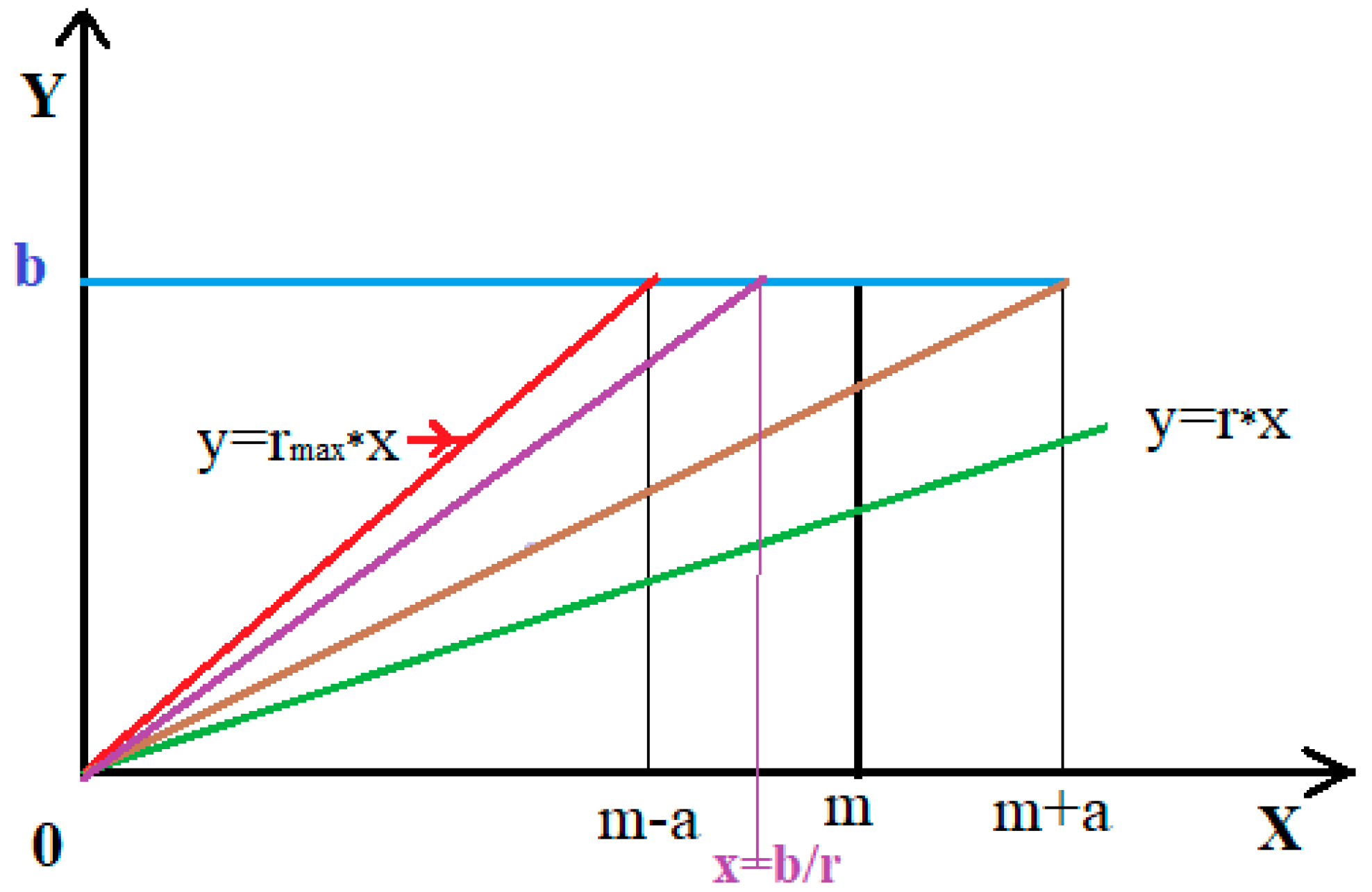
Figure 2.
Representative images collected from tailings pond Teliuc, Romania: a) access way to the pond; b) edge with boulders and minor rock; c) marginal grass and lack of vegetation on the pond; d) lunar aspect; e) detailed on lunar aspect; b) solid lumpy waste.
Figure 2.
Representative images collected from tailings pond Teliuc, Romania: a) access way to the pond; b) edge with boulders and minor rock; c) marginal grass and lack of vegetation on the pond; d) lunar aspect; e) detailed on lunar aspect; b) solid lumpy waste.
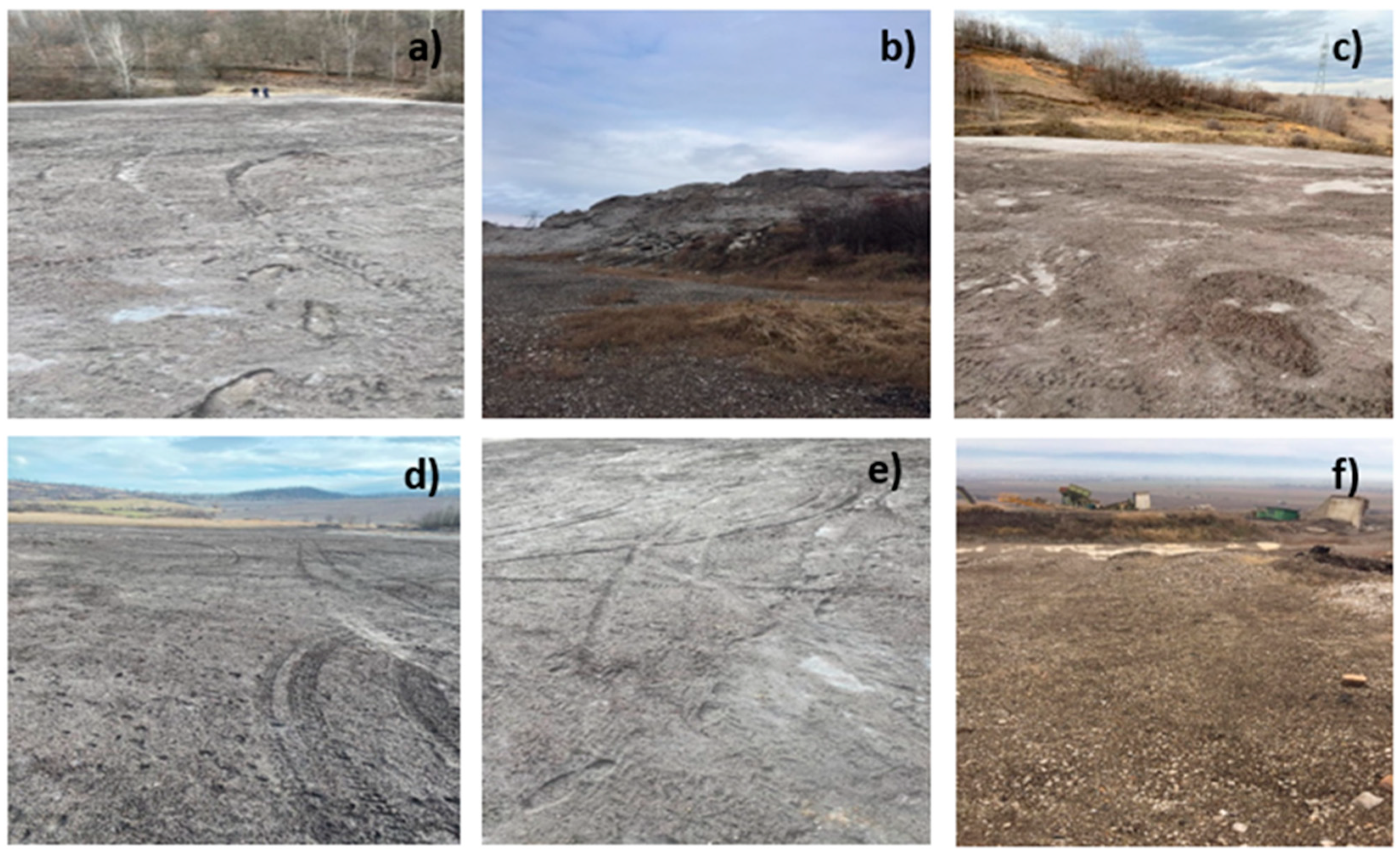
Figure 3.
Images regarding incremental sampling: a) sampling from a depth of 50 cm; b) fine waste sample; c) coarse waste sample.
Figure 3.
Images regarding incremental sampling: a) sampling from a depth of 50 cm; b) fine waste sample; c) coarse waste sample.
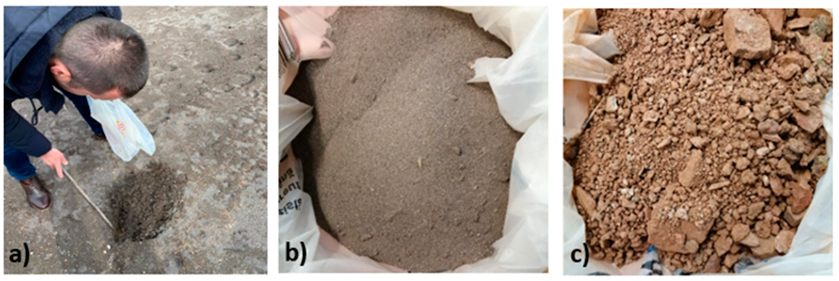
Figure 4.
Representative SEM images of the sampled tailings: a) an image of the fine particles; b) image of an aggregate of particles; c) image showing a rugged surface morphology of tailings; d) image specific to crystalline particles;.
Figure 4.
Representative SEM images of the sampled tailings: a) an image of the fine particles; b) image of an aggregate of particles; c) image showing a rugged surface morphology of tailings; d) image specific to crystalline particles;.
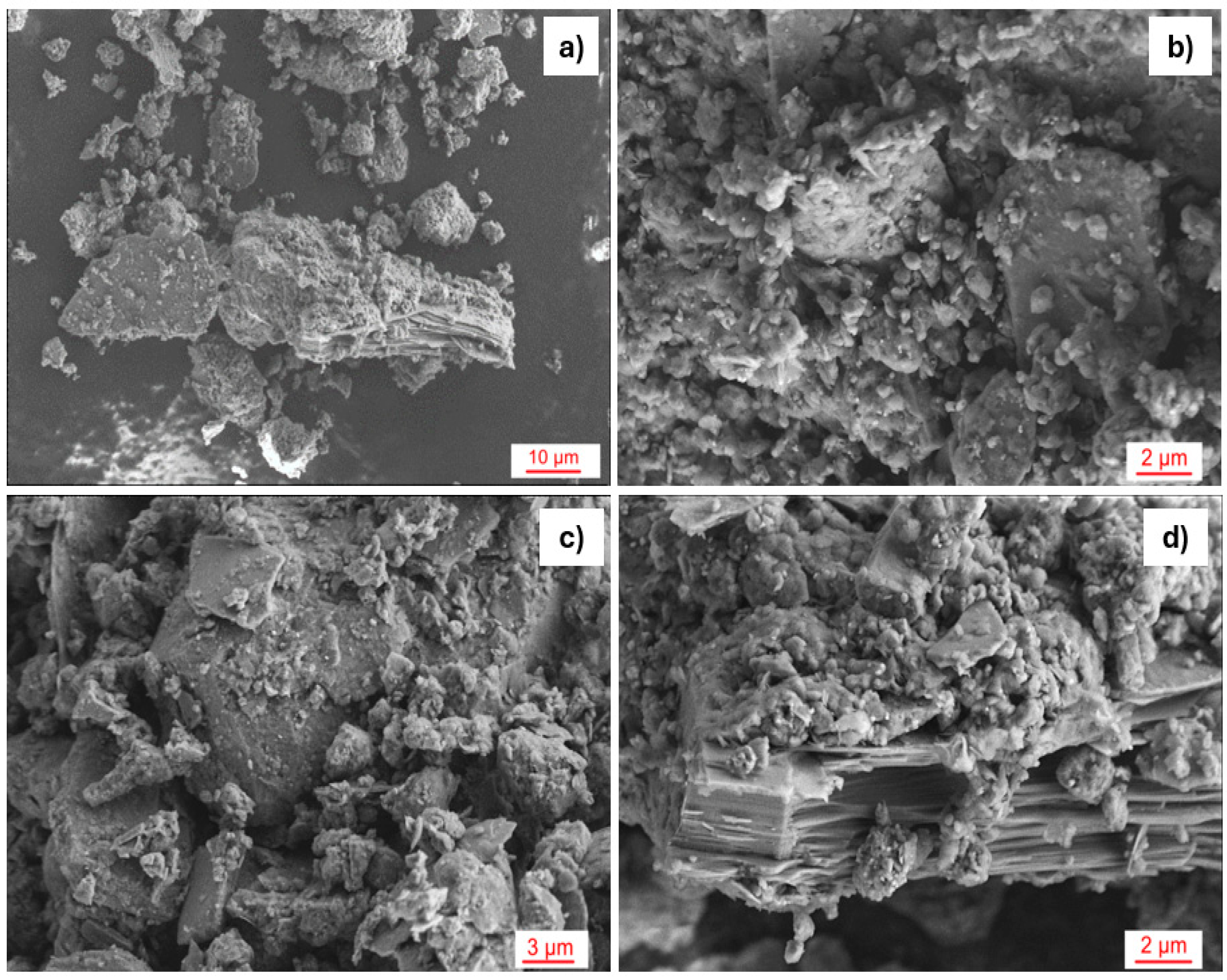
Figure 5.
EDS spectra associated to Figure 4 and elemental analyses associated with each spectrum: a) EDS spectrum associated with Figure 4 b); b) EDS spectrum associated with Figure 4 d.
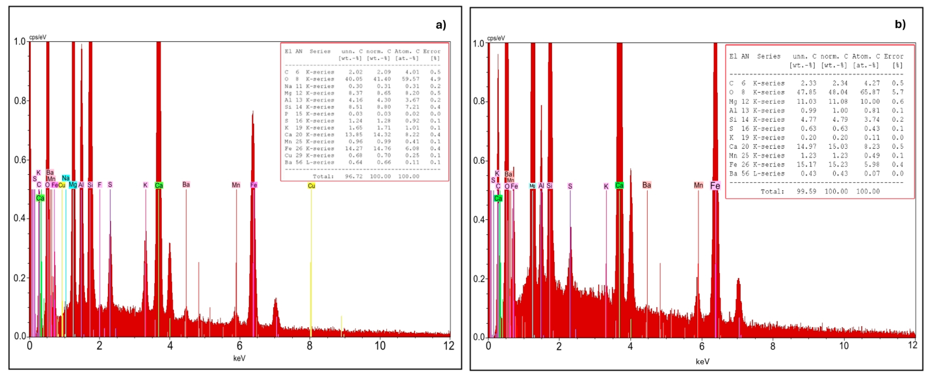
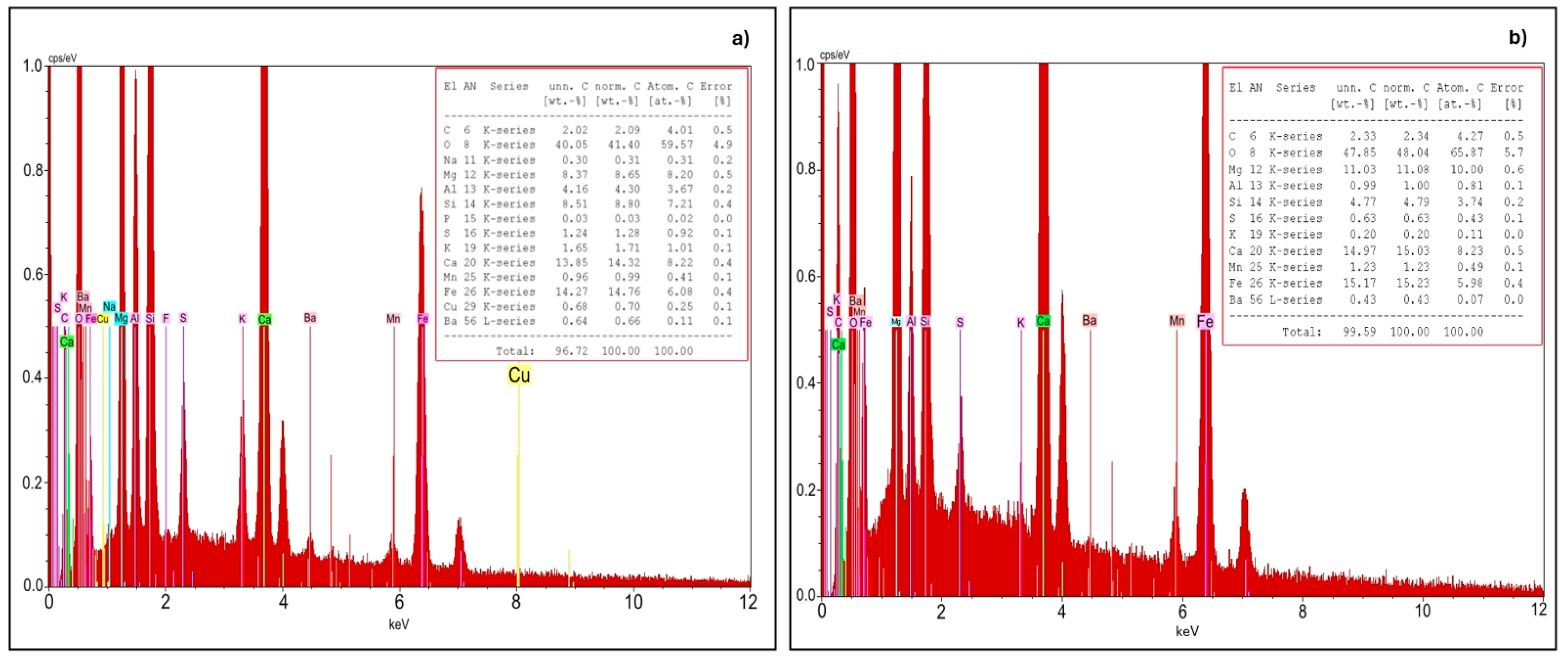
Figure 6.
Histograms of the concentration values in ppm for: a) Y and b) Ce.
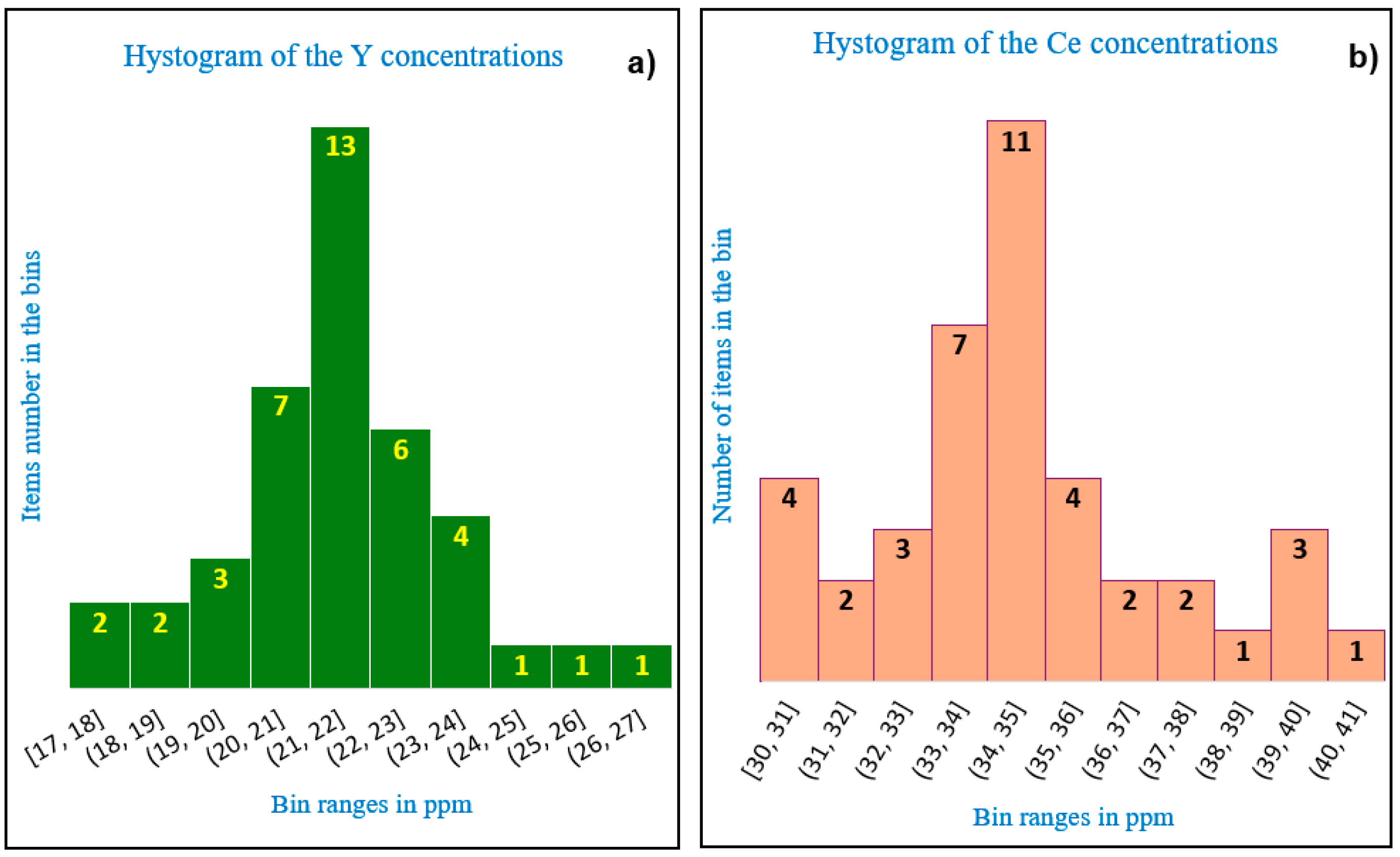
Figure 7.
Histograms of the concentration values in ppm for: a) Ge and b) Bi.
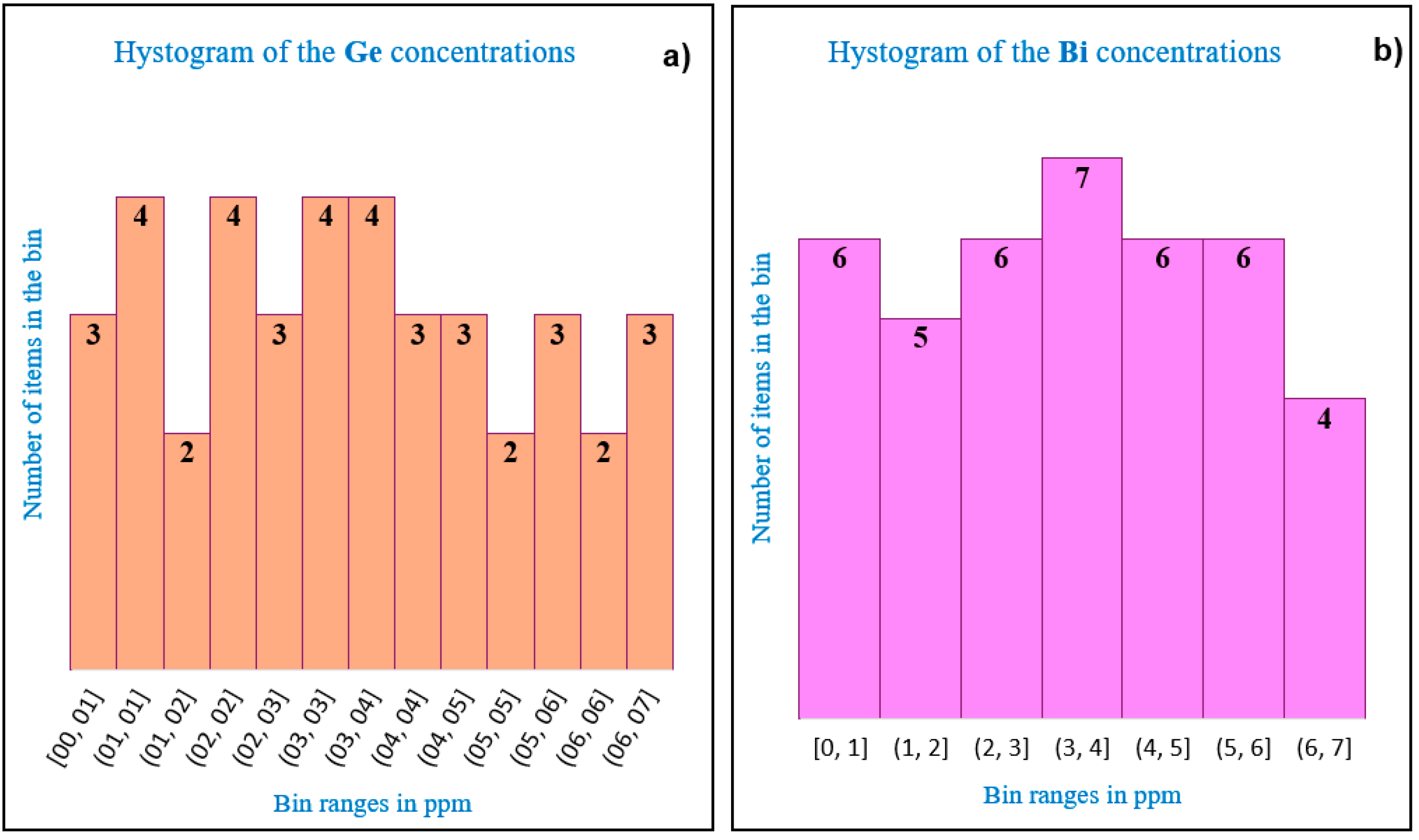

Table 1.
Representative XRFS Test Report for aliquots no. 1 and no. 22 belonging to the sampling set of 40 samples.
Table 1.
Representative XRFS Test Report for aliquots no. 1 and no. 22 belonging to the sampling set of 40 samples.
| Description Method - TurboQuant-Pelette | |||||
| Aliquot no. 1 | Aliquot no. 22 | ||||
| Z | Symbol | Concentration [%wt.] |
*SD [%wt.] |
Concentration [%wt.] |
SD [%wt.] |
| 11 | Na2O | 0.804056 | 0.024000 | 1.794032 | 0.023658 |
| 12 | MgO | 1.344708 | 0.009000 | 1.358216 | 0.007707 |
| 13 | Al2O3 | 9.817325 | 0.010000 | 9.686015 | 0.009131 |
| 14 | SiO2 | 52.68028 | 0.0300 | 49.572850 | 0.032995 |
| 15 | P2O5 | 0.642814 | 0.001700 | 0.642621 | 0.001823 |
| 16 | SO3 | 2.324803 | 0.000900 | 3.449874 | 0.000920 |
| 17 | Cl | 0.014883 | 0.000070 | 0.014575 | 7.19E-05 |
| 19 | K2O | 2.030205 | 0.006000 | 2.188351 | 0.005578 |
| 20 | CaO | 11.38931 | 0.00900 | 14.88444 | 0.008529 |
| 22 | TiO2 | 0.855457 | 0.004500 | 0.812547 | 0.004797 |
| 23 | V2O5 | 0.01414 | 0.00130 | 0.013785 | 0.001213 |
| 24 | Cr2O3 | 0.025996 | 0.000460 | 0.024948 | 0.000407 |
| 25 | MnO | 0.11524 | 0.00070 | 0.113313 | 0.000781 |
| 26 | Fe2O3 | 15.62105 | 0.00400 | 13.89942 | 0.003672 |
| 27 | CoO | 0.001607 | 0.000230 | 0.001600 | 0.000234 |
| 28 | NiO | 0.006846 | 0.000100 | 0.006134 | 0.00011 |
| 29 | CuO | 0.025287 | 0.000150 | 0.026669 | 0.000158 |
| 30 | ZnO | 0.125794 | 0.000300 | 0.120923 | 0.000281 |
| 31 | Ga | 0.001243 | 0.000040 | 0.001316 | 3.63E-05 |
| 32 | Ge | 0.000461 | 0.000040 | 0.000172 | 0.000040 |
| 33 | As2O3 | 0.000866 | 0.000090 | 0.000789 | 9.10E-05 |
| 34 | Se | 5.06E-05 | 0.00002 | 0.00005 | 2.05E-05 |
| 35 | Br | 0.001244 | 0.000020 | 0.00134 | 2.03E-05 |
| 37 | Rb2O | 0.00869 | 0.00003 | 0.007784 | 3.21E-05 |
| 38 | SrO | 0.016866 | 0.000040 | 0.018128 | 3.56E-05 |
| 39 | Y | 0.002172 | 0.000030 | 0.001990 | 3. 20E-05 |
| 40 | ZrO2 | 0.029554 | 0.000240 | 0.028678 | 0.000240 |
| 41 | Nb2O5 | 0.001186 | 0.000070 | 0.00122 | 6.65E-05 |
| 42 | Mo | 0.000831 | 0.000060 | 0.00081 | 6.38E-05 |
| 47 | Ag | 0.000535 | 0.000160 | 0.000530 | 0.000152 |
| 48 | Cd | 0.000398 | 0.000060 | 0.000410 | 5.50E-05 |
| 50 | SnO2 | 0.002718 | 0.000130 | 0.002817 | 0.000137 |
| 51 | Sb2O5 | 0.000882 | 0.000110 | 0.000900 | 0.000118 |
| 52 | Te | < 0.00030 | - | < 0.00030 | - |
| 53 | I | < 0.00030 | - | < 0.00030 | - |
| 55 | Cs | 0.000953 | 0.000590 | 0.000950 | 0.000532 |
| 56 | Ba | 0.069997 | 0.001000 | 0.062817 | 0.000879 |
| 57 | La | < 0.00020 | - | < 0.00020 | - |
| 58 | Ce | 0.003449 | 0.000760 | 0.003740 | 0.000840 |
| 72 | Hf | 0.00055 | 0.00007 | 0.000531 | 6.85E-05 |
| 73 | Ta2O5 | < 0.00063 | - | < 0.00063 | - |
| 74 | WO3 | 0.001896 | 0.000140 | 0.001834 | 0.000129 |
| 79 | Au | 0.000131 | 0.000060 | - | - |
| 80 | Hg | < 0.00010 | - | < 0.00010 | - |
| 81 | Tl | 0.000117 | 0.000020 | 0.00012 | 2.16E-05 |
| 82 | PbO | 0.021109 | 0.000100 | 0.0233090 | 0.000108 |
| 83 | Bi | 0.000172 | 0.000060 | < 0.00010 | - |
| 90 | Th | 0.000883 | 0.000040 | 0.000888 | 3.81E-05 |
| 92 | U | 6.94E-05 | 0.00001 | 6.51E-05 | 8.92E-06 |
| Total | 99.21829 | 98.7713 | |||
*SD-measurement standard deviation of the XRFS laboratory procedure.
Table 2.
Concentration (C) and associated standard deviation (SD) of Y, Ce, Ge and Bi in ppm, measured through ED(P)-XRFS on the 40 sampled tailings aliquots.
Table 2.
Concentration (C) and associated standard deviation (SD) of Y, Ce, Ge and Bi in ppm, measured through ED(P)-XRFS on the 40 sampled tailings aliquots.
| Sample No |
Y | Ce | Ge | Bi | ||||
|---|---|---|---|---|---|---|---|---|
| C | SD | C | SD | C | SD | C | SD | |
| 1 | 21.70 | 0.30 | 34.50 | 7.60 | 4.60 | 0.41 | 1.70 | 0.70 |
| 2 | 21.50 | 0.30 | 32.10 | 8.00 | 5.10 | 0.40 | 0.00 | 0.00 |
| 3 | 26.20 | 0.30 | 30.00 | 8.00 | 2.60 | 0.40 | 2.60 | 0.70 |
| 4 | 25.40 | 0.30 | 30.00 | 7.00 | 2.20 | 0.40 | 3.10 | 0.60 |
| 5 | 21.55 | 0.30 | 34.39 | 7.60 | 0.00 | 0.00 | 4.40 | 0.60 |
| 6 | 21.88 | 0.30 | 33.98 | 7.53 | 0.80 | 0.41 | 4.05 | 0.60 |
| 7 | 21.32 | 0.30 | 33.30 | 7.51 | 1.70 | 0.40 | 0.00 | 0.00 |
| 8 | 22.30 | 0.30 | 35.00 | 7.67 | 1.80 | 0.40 | 1.80 | 0.60 |
| 9 | 21.55 | 0.30 | 34.39 | 7.60 | 3.55 | 0.40 | 3.21 | 0.60 |
| 10 | 21.88 | 0.30 | 33.30 | 7.51 | 3.20 | 0.40 | 4.22 | 0.60 |
| 11 | 21.32 | 0.30 | 33.98 | 7.53 | 3.60 | 0.40 | 5.40 | 0.60 |
| 12 | 22.30 | 0.30 | 32.50 | 7.67 | 2.63 | 0.40 | 5.60 | 0.60 |
| 13 | 21.00 | 0.30 | 35.00 | 8.60 | 1.30 | 0.40 | 3.80 | 0.60 |
| 14 | 21.88 | 0.30 | 33.98 | 7.53 | 4.10 | 0.40 | 3.20 | 0.60 |
| 15 | 21.00 | 0.30 | 32.50 | 8.60 | 3.20 | 0.40 | 0.00 | 0.00 |
| 16 | 21.00 | 0.30 | 35.00 | 8.30 | 2.12 | 0.40 | 4.50 | 0.60 |
| 17 | 21.18 | 0.33 | 34.50 | 8.60 | 4.10 | 0.42 | 3.40 | 0.60 |
| 18 | 21.18 | 0.31 | 34.50 | 8.05 | 3.35 | 0.45 | 4.10 | 0.60 |
| 19 | 21.18 | 0.36 | 34.50 | 7.60 | 5.54 | 0.42 | 2.30 | 0.60 |
| 20 | 21.18 | 0.33 | 34.50 | 8.42 | 5.74 | 0.42 | 0.00 | 0.00 |
| 21 | 19.50 | 0.32 | 30.30 | 8.25 | 5.10 | 0.42 | 1.40 | 0.80 |
| 22 | 19.90 | 0.32 | 37.40 | 8.39 | 0.91 | 0.42 | 0.00 | 0.00 |
| 23 | 18.80 | 0.29 | 31.60 | 7.54 | 0.00 | 0.00 | 5.20 | 0.56 |
| 24 | 23.60 | 0.30 | 38.00 | 8.24 | 1.09 | 0.42 | 5.10 | 0.80 |
| 25 | 18.70 | 0.32 | 39.10 | 8.49 | 2.40 | 0.42 | 2.10 | 0.50 |
| 26 | 17.70 | 0.30 | 39.70 | 7.60 | 0.87 | 0.42 | 1.90 | 0.50 |
| 27 | 20.20 | 0.31 | 36.50 | 7.76 | 0.76 | 0.42 | 3.80 | 0.60 |
| 28 | 20.00 | 0.33 | 35.40 | 8.39 | 2.63 | 0.42 | 3.60 | 0.60 |
| 29 | 16.19 | 0.40 | 30.40 | 8.05 | 4.50 | 0.42 | 2.30 | 0.40 |
| 30 | 20.50 | 0.30 | 34.40 | 8.40 | 1.07 | 0.42 | 4.50 | 0.60 |
| 31 | 23.60 | 0.30 | 33.90 | 7.91 | 1.25 | 0.42 | 0.00 | 0.00 |
| 32 | 20.40 | 0.29 | 35.80 | 7.79 | 0.00 | 0.00 | 6.50 | 0.70 |
| 33 | 20.20 | 0.30 | 35.20 | 7.00 | 0.62 | 0.43 | 2.36 | 0.97 |
| 34 | 22.90 | 0.30 | 31.80 | 7.10 | 3.60 | 0.42 | 6.22 | 1.00 |
| 35 | 22.40 | 0.32 | 35.20 | 7.64 | 2.73 | 0.42 | 2.23 | 1.03 |
| 36 | 23.70 | 0.31 | 33.40 | 7.77 | 0.00 | 0.00 | 1.97 | 1.00 |
| 37 | 22.20 | 0.29 | 36.20 | 7.55 | 1.02 | 0.42 | 6.15 | 1.04 |
| 38 | 23.30 | 0.30 | 40.20 | 8.10 | 1.83 | 0.42 | 5.36 | 1.10 |
| 39 | 24.30 | 0.27 | 39.90 | 7.40 | 0.00 | 0.00 | 2.30 | 0.97 |
| 40 | 22.30 | 0.33 | 38.50 | 7.36 | 1.48 | 0.42 | 5.35 | 1.00 |
Table 3.
The outcomes of statistical data analyses through classical, robust and conservative approaches.
Table 3.
The outcomes of statistical data analyses through classical, robust and conservative approaches.
| Statistical parameters | Y | Ce | Ge | Bi |
| Classical statistical analysis of the data | ||||
| Arithmetic mean [ppm] | 22.01 | 36.50 | 3.54 | 3.05 |
| SD [ppm] | 1.85 | 2.62 | 1.97 | 1.82 |
| RSD (%) | 8 | 7 | 56 | 60 |
| Robust statistical analysis of the data | ||||
| Median [ppm] | 21.41 | 34.50 | 3.31 | 2.88 |
| SD* [ppm] | 0.89 | 2.97 | 2.69 | 2.32 |
| RSD* (%) | 4 | 9 | 81 | 81 |
| Conservative data analysis | ||||
| Mean [ppm] | 11.15 | 19.25 | 2.31 | 2.68 |
| LOQ [ppm] | 0.50 | 1.00 | 0.50 | 1.00 |
| Uncertainty [ppm] | 9.12 | 15.75 | 1.95 | 2.40 |
| Relative uncertainty (%) | 82 | 82 | 84 | 90 |
Disclaimer/Publisher’s Note: The statements, opinions and data contained in all publications are solely those of the individual author(s) and contributor(s) and not of MDPI and/or the editor(s). MDPI and/or the editor(s) disclaim responsibility for any injury to people or property resulting from any ideas, methods, instructions or products referred to in the content. |
© 2025 by the authors. Licensee MDPI, Basel, Switzerland. This article is an open access article distributed under the terms and conditions of the Creative Commons Attribution (CC BY) license (http://creativecommons.org/licenses/by/4.0/).
Copyright: This open access article is published under a Creative Commons CC BY 4.0 license, which permit the free download, distribution, and reuse, provided that the author and preprint are cited in any reuse.


