Hardware‐Based Open Switch Fault Diagnosis in Three‐Phase Voltage Source Inverters Using Single Neuron Implementation

1. Introduction

Nowdays, DC-AC converters have been effectively used in industrial equipment like adjustable speed drives, uninterruptible power supplies, flexible AC transmission systems, voltage compensators, photovoltaic inverters, and others [1]. DC-AC converters have advantages like high effectiveness, high accuracy, compactness, and high consistency. The consistency of the DC-AC converters is a most important disquiet. The fault-tolerant control to guarantee the uninterrupted and correct converter operation is compulsory [2]. This involves a quick and consistent fault diagnostic system. It is observed that the switching devices in the power converter are one of the weakest components, which report about 30% of the breakdown and cause interruptions [3].

Induction Motors (IMs) are driven by the space vector control approach and the process to be followed in controls is utilized by Voltage Source Inverter (VSI) [4]. However, as a result of the complications of the drive systems and the diversity of operation conditions, several faults take place in the VSI. When there are faults in the VSI, the whole induction motor drive system will not function under normal or usual conditions [5]. Moreover, the faults occurred in control techniques can affect financial losses or terrible accidents [6]. As a result, an investigation of the fault diagnosis in the VSI is the most significant.

The core components involved in power conversion are power switches such as Insulated Gate Bipolar Transistors (IGBT) or Metal Oxide Semiconductor Field Effect Transistors (MOSFET). It is well-known that there are six power switches in the three-phase VSI. The breakdown of these power switches can be broadly classified as short circuit faults (SCFs), Misfiring Faults (MFs), and Open-Circuit Faults (OCFs) [7].

The SCFs take place rapidly and IGBT can sustain against this fault for 10 µsec [8]. Hence, it is hard to identify SCFs using algorithmic techniques as protection time is very small. MFs are caused due to missing transistor gate pulses which result in poor performance of devices. Several methods should be utilized to diagnose OCFs[9]. As a result, much of that current research is going in the area of OCF diagnosis in the VSI, which is furthermore the research topic in this paper. Out of several open circuit Faultdiagnostic Methods(FDMs) of switching devices in power converters, Park’s Vector Transform (PVT)based diagnosis techniques have received a lot of interest in the past few decades. M. Trabelsi et al. proposed OCF diagnosis in the two power converters of a Permanent Magnet Synchronous Generators (PMSGs) drive for the online diagnosis of multiple OCFs. This has been implemented signal processing algorithms on the dSPACE DS1103 digital controller that needs only three-phase current and speed which are already sensed for internal control of the drive. The FDM shows high resistance to false alarms, sustaining under variable load or high-speed conditions[10].

Current trajectory’s midpoint [11], Normalized DC Current Method[12], Modified Normalized DC Current Method [13], and Slope Method [14] are based on PVT and have been implemented on MATLAB and Xmath package for diagnosis of OCF.

The author proposed in [15] the FDM for a three-phase Permanent Magnet Synchronous Motor (PMSM) drive based on the average current calculated using PVT. The Fault Diagnosis Variables (FDVs) are computed by using the average current. The Fuzzy based classifier is applied to process the FDVs to diagnose single or multiple OCFs with 96% accuracy. The algorithm is implemented on DSP (TMS320F2812) control board. A combination of PVT and Fuzzy Logic System (FLS) has been proposed in [16] for the diagnosis of single and multiple OCF under variable load conditions. The FLS is utilized for a threshold value adjustment to diagnose OCF under variable load conditions.

R. B. Dhumale, et al. proposed FDM based on the combination of signal preprocessing, feature extraction, feature selection technique, and fault classifier. The PVT is used to normalize current to diagnose fault under variable load conditions [17]. The features are extracted using Discrete Wavelet Transform (DWT) and max features are selected to train the Artificial Neural Network (ANN) based fault classifier. The results are shown for different fault patterns, single and multiple OCFs under variable load conditions at different frequencies. Also, the results are shown for the online fault diagnosis, with the incidence of fault occurrence and the incidence of diagnosis. This method requires Digital Signal Controller for the implementation of the proposed FDM as a result this algorithmic solution requires high processing time. An easy and reliable method for the diagnosis of OCFs based on a discrete wavelet transform (DWT) and the FLS has been proposed in [18]. The proposed FDM is checked for a variable load condition and experimental results are validated on dsPIC30F4011. In contrast, this technique is slower than other earlier proposed FDMs but gives satisfactory results for practical applications. The same combination of DWT-FLS has been implemented on an Intel 80C196KC 16-bit microcontroller for the diagnosis of single switch faults in Pulse Width Modulation (PWM)-VSI. This FDM shows a high potential for OCF diagnosis[19].

In [20] author proposed Artificial Neural Network (ANN) based FDM, four features like two-phase currents (I_α and I_β), angle to the current pattern (I_θ), and surface difference of the current patterns between healthy and faulty (E_s) are extracted from the current signal using PVT. An ANN of structure 4-15-13 is implemented onthe computerfor further processing. This FDM is quick, capable, and 100% perfect for single or multiple OCF diagnoses. The single and multiple OCF diagnoses of a phase-controlled three-phase full-bridge rectifier using the Deep Neural Network (DNN) have been proposed in [21]. Wavelet-Neural Network Method, Wavelet-ANFI System, Clustering-ANFI method, and Model-Based ANN Method have been proposed in [22,23,24,25] respectively. Simulation results show great accuracy of fault classification using ANN. Some manual methods have been proposed in [26,27] which are based on measured voltage and Bond Graph Model respectively. In [28], the current spectrum has been examined for the diagnosis of OCF. A Fast Fourier Transform (FFT) has been analyzed for the spectrum analysis. This needs comparatively high computing power.

The main disadvantages of the earlier techniques were the load dependence and the sensitivity to transients, whereas the drawbacks are overcome in recently proposed FDMs in review [10,15,16,17]. These recent methods have good efficiency for low load levels and during transients. The normalized average currents are proposed and processed to succeed in dealing with these limitations. As per the reviews and surveys in the literature, it is observed that several FDMs for OCFs in VSIs have been proposed but these methods are complicated and require either a DSP control board or computer for practical implementation. Therefore, the objective of this research paper is to propose an innovative idea to investigate new FDM based on fundamental hardware components. The Hardware-based Implementation of the Single Neuron Algorithm (HISNA) for Open Switch Fault Diagnosis in VSI is explained in section II, where the implementation of the proposed HISNA is reported in section III, and experimental results are presented to evaluate the fault diagnosis performance in section IV.

This research introduces a new online Fault Diagnosis System (FDS) for detecting OCF in switches using a Hardware-Based Intelligent Single Neuron Approach (HISNA). Unlike other methods, it does not require extra hardware like a DSP control board or a computer for practical use. A detailed study of existing research was done to understand the need for a simple hardware-based fault diagnosis system for Permanent Magnet Synchronous Motor (PMSM) drives working under different load conditions. The system is designed using a single-neuron ANN model, which can diagnosis all types of open-circuit faults, including single-phase faults, in PMSM drives. Additionally, the input and bias weights are carefully chosen by studying how different fault conditions affect the system under changing load conditions. This ensures accurate and reliable fault diagnosis.

2. Fault Diagnostic Method

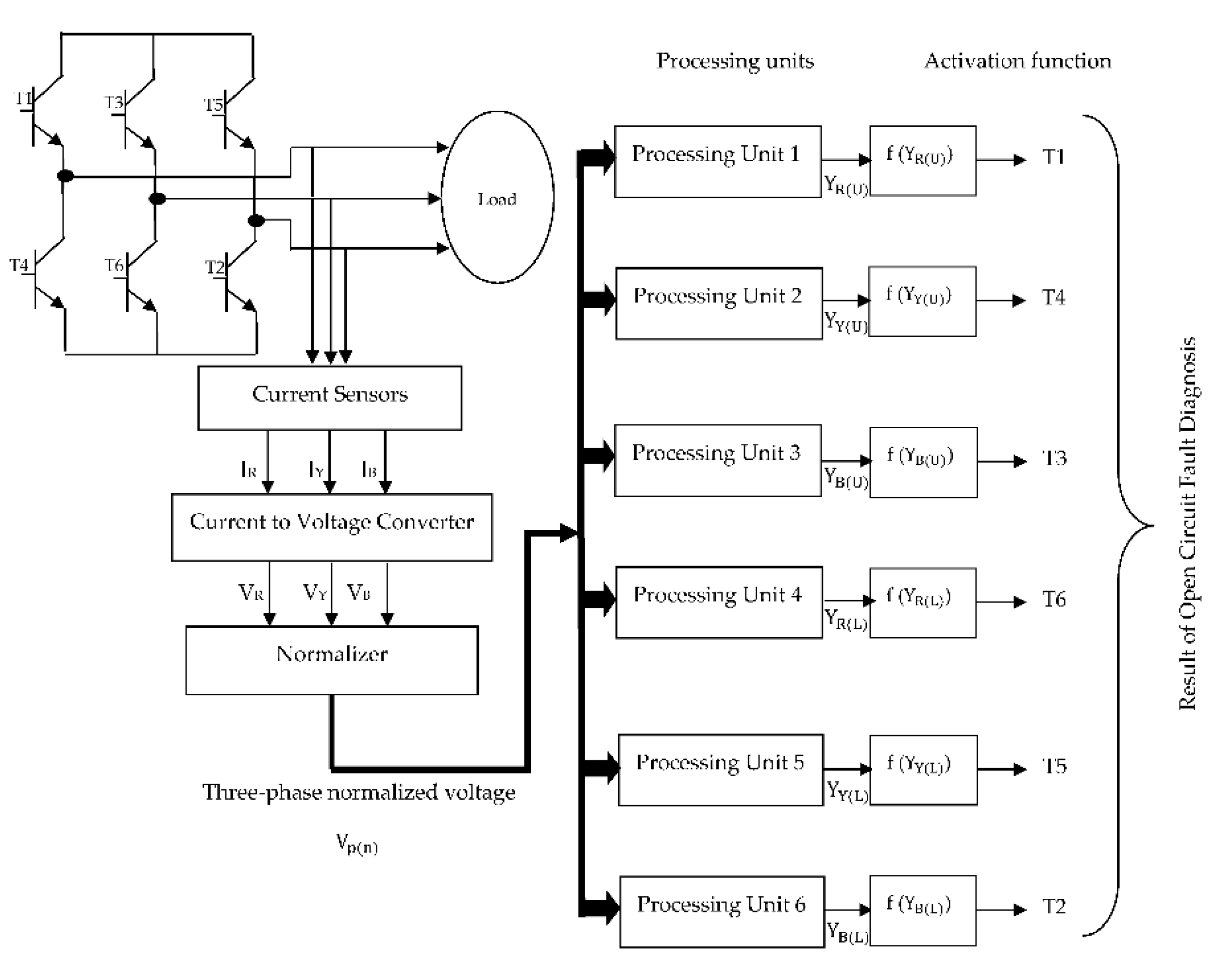
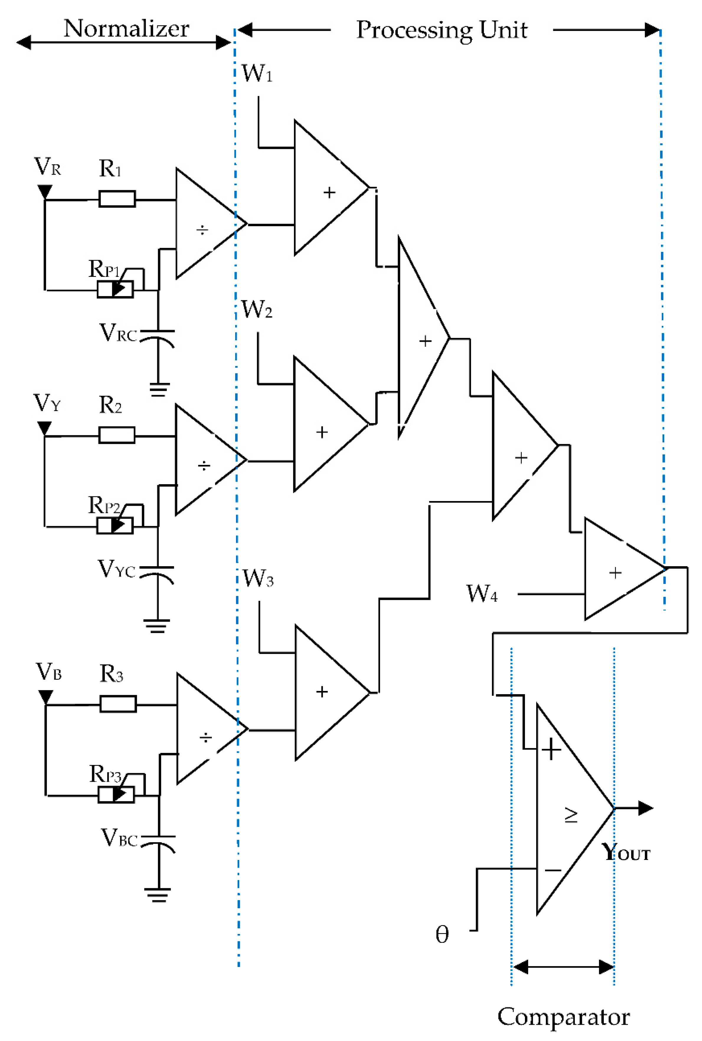
The structure of a VSI consists of six transistors; two transistors for each phase. The supply from AC mains is converted into DC using a bridge rectifier and filter. This DC input is provided to each of these transistors in a typical switching manner to generate the three-phase voltage used to drive the load. The circuit diagram of the three-phase inverter is shown in Figure 1. The current signals at the output of each phase of VSI are sensed and converted into voltage using a V-I converter. In the proposed HISNA system, the extracted signal is given by Eq. 1.

$${\mathrm{V}}_{\mathrm{p}}=\mathrm{}{\mathrm{V}}_{\mathrm{m}}\mathrm{}\times \mathrm{s}\mathrm{i}\mathrm{n}\left(\mathsf{\omega }\mathrm{t}\right)\mathrm{}\mathrm{}$$

(1)

Where V_p is the output of VSI, and p is phase R, Y, or B. V_m is the Peak value of the signal and ω is the angular frequency. The sensed signals are normalized so that the system can diagnose fault under variable load conditions. In the normalization process, sensed signals are divided by the peak value of that signal which is given by Eq. 2.

$${\mathrm{V}}_{\mathrm{p}\left(\mathrm{n}\right)}={\displaystyle \frac{{\mathrm{V}}_{\mathrm{m}}\times \left(\mathrm{s}\mathrm{i}\mathrm{n}\left(\mathsf{\omega }\mathrm{t}\right)\right)}{{\mathrm{V}}_{\mathrm{m}}}}$$

(2)

Where V_p(n) is the output of the normalizer. The normalized signal is further applied to the processing unit which is also called neuron cells. In ANN, the basic computational element is called a neuron cell or processing unit. It receives input through the synaptic terminals each having an associated weight with it. A single artificial neuron cell has been used for the classification of the faulty switch. In the HISNA system, six neuron cells are implemented for six switches as shown in Fig.1. A neuron cell classifies faulty switches from the same phase. I_p(n) and bias ($\mathrm{b}$) are two inputs to the neuron cell having corresponding weights as W_p and W_0p respectively.

The neuron cell or processing unit uses the equation to calculate output as given in Eq. 3.

$${\mathrm{Y}}_{\mathrm{p}\left(\mathrm{s}\right)}={\mathrm{W}}_{\mathrm{R}}\times {\mathrm{V}}_{\mathrm{R}\left(\mathrm{n}\right)}+{{\mathrm{W}}_{\mathrm{Y}}\times {\mathrm{V}}_{\mathrm{Y}\left(\mathrm{n}\right)}+{\mathrm{W}}_{\mathrm{B}}\times {\mathrm{V}}_{\mathrm{B}\left(\mathrm{n}\right)}+\mathrm{b}\times \mathrm{W}}_{0\mathrm{p}}$$

(3)

Y_P(S) is the output of ANN for the individual switch. S is a parameter showing the Upper or Lower switch. U stands for the upper switch and L for the lower switch in phase. W_P and W_0P are the pre-determined synaptic weights for each switch. ${\mathrm{W}}_{\mathrm{R}},{\mathrm{W}}_{\mathrm{Y}},and{\mathrm{W}}_{\mathrm{B}}$ are the calculated weights of neuron cells of R, Y, and B phases respectively.

The normalized signal at the output of the normalizer is multiplied with a pre-determined synaptic weight. The product obtained is added with a pre-determined bias to implement Eq. 3. The values of the synaptic weights are calculated by training ANN using Delta Learning Rule. The Gradient Descent Algorithm is used to calculate optimum values of parameters by minimizing the Cost Function (C_F) given by Eq. 4.

$${\mathrm{C}}_{\mathrm{F}}={\displaystyle \frac{1}{\mathrm{n}}}\sum _{\mathrm{p}=0}^{\mathrm{n}}{({\mathrm{Y}}_{\mathrm{p}\left(\mathrm{n}\right)}-{\mathrm{Y}}_{\mathrm{w}})}^2$$

(4)

Y_W is the actual output for ${\mathrm{p}}^{\mathrm{t}\mathrm{h}}$ training sample. The term $\left(Y_{p\left(n\right)}-Y_w\right)$ is for calculating the difference between the actual value and fitted value of the ${\mathrm{p}}^{\mathrm{t}\mathrm{h}}$ training example. The cause that squaring is to eliminate the sign earlier to this error as it can be both positive and negative. The new weights are calculated by using weight updating equations given in Eq. 5 and Eq. 6.

$${\mathrm{W}}_{\mathrm{p}\mathrm{s}}={\mathrm{W}}_{\mathrm{p}\mathrm{s}}+\mathrm{}\mathrm{ɳ}\times {\displaystyle \frac{1}{\mathrm{n}}}\sum _{\mathrm{p}=0}^{\mathrm{n}}\left({\mathrm{Y}}_{\mathrm{p}\left(\mathrm{s}\right)}-{\mathrm{Y}}_{\mathrm{w}}\right)\times {\mathrm{X}}_{\mathrm{p}}$$

(5)

$${\mathrm{W}}_{0\mathrm{p}}={\mathrm{W}}_{0\mathrm{p}}+\mathrm{}\mathrm{ɳ}\times {\displaystyle \frac{1}{\mathrm{n}}}\sum _{\mathrm{p}=0}^{\mathrm{n}}\left({\mathrm{Y}}_{\mathrm{p}\left(\mathrm{s}\right)}-{\mathrm{Y}}_{\mathrm{w}}\right)$$

(6)

Where ɳ is the learning rate which is a parameter that decides to what extent the new weights change concerning old values. The activation function is a function that is used to map the output of ANN Y_P(S) into a response variable based on a decision. The threshold activation function is used to convert process value ${\mathrm{Y}}_{\mathrm{p}\left(\mathrm{S}\right)}$ into a decision which is given by Eq. 7.

$${\mathrm{}\mathrm{T}}_{\mathrm{j}}=\mathrm{f}\left({\mathrm{Y}}_{\left(\mathrm{P}\mathrm{S}\right)}\right)=\mathrm{}\left\{\begin{array}{c}0{\mathrm{}\mathrm{Y}}_{\mathrm{p}\left(\mathrm{S}\right)}<\theta \\ 1{\mathrm{}\mathrm{}\mathrm{Y}}_{\mathrm{p}\left(\mathrm{S}\right)}>\theta \end{array}\right.\mathrm{}\mathrm{}$$

(7)

J is 1, 2, 3,..,6 and θ is the threshold value. The value of $\mathsf{\theta }$ is determined by observing the output ${\mathrm{Y}}_{\mathrm{p}\left(\mathrm{S}\right)}$ which is given by Eq. 3. The output of the processing unit is provided as an input to the activation function which compares it with a threshold value. The output of the activation function is ‘1’ if the fault is present in the switch and ‘0’ for the healthy condition.

3. Implementation

An open-circuit fault in the VSI is introduced by opening the collector terminal in the experimental setup for the proposed HISNA system. Such a facility is generated in the test box. The Data Acquisition System (DAS) consists of a VSI, induction motor, and real-time interface. A protection circuit is provided to avoid the damage to the IGBTs, caused due to various faulty conditions. The specifications of VSI used in experimentation are given in Table 1. The variable load conditions are implemented in the test bench for its application during the proposed methodology assessment using a pulley wheel mechanism which helps to increase or decrease the load on the induction motor. 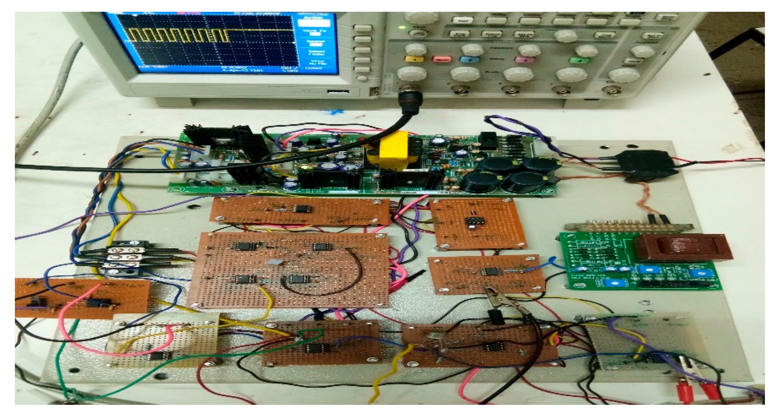An induction motor with 0.75kW, 1415 rpm, and 1.8 Amp current rating is used for experimentation. The features like analog to digital converter and Pulse Width Modulation of DSP processor TMS320C2407 are used. The experimental setup is shown in Figure 2.A. The three-phase AC signal at the output of the inverter is passed through a filter circuit. These individual phase signals are normalized within the range of ‘±1’ to avoid the effect of load variation.

The normalized signal is used to train ANN which is implemented by the equation Eq.3. The values of weights W_p and W_0p are calculated using Gradient Descent Algorithm implemented using MATLAB as given below.

• Load training data as input vector ${\mathrm{V}}_{\mathrm{p}\left(\mathrm{n}\right)}$ and their expected output vector$Y_w$. Initialize weights (${\mathrm{W}}_{\mathrm{p}}$and${\mathrm{W}}_{0\mathrm{p}}$), number of iterations, learning rate (η), and cost function (C_f).
• Calculate value of new weights using Eq.5 & Eq.6.
• Calculate values of the ${\mathrm{Y}}_{\mathrm{p}\left(\mathrm{s}\right)}$ using equation Eq.3.
• Calculate values of the cost function using equation Eq.4.
• Repeat steps 3, 4, and 5 for the given number of iterations or till getting the required value of C_f.

A separate processing unit for each switch is implemented to diagnose OCF in the switch. To implement the HISNA system, samples of health conditions and samples with faulty conditions have been combined. For the information that is collected to diagnose the fault in T1, combinations like T1, T1-T2, T1-T3, T1-T4, T1-T5, and T1-T6 have been taken. Such information is collected for other switches. For example, the combination of T2, T2-T1, T2-T3, T2-T4, T2-T5, and T2-T6. In this way, such six sets for the six switches have been made. Different values for ${\mathrm{W}}_{\mathrm{p}}$and${\mathrm{W}}_{0\mathrm{p}}$ are calculated for each set. The algorithm above is used to find it. The calculated weights are substituted in Eq. 3 to obtain the output.

The ANN model is trained for 10000 iterations with a 0.007 learning rate which is obtained by trial and error. The parameters ${\mathrm{W}}_{\mathrm{p}}$and${\mathrm{W}}_{0\mathrm{p}}$ obtained during the implementation of the HISNA system are given inTable 2. By putting these values of weights in Eq. 3 and looking at the healthy condition of the switch, the maximum value of ${\mathrm{Y}}_{\mathrm{p}\left(\mathrm{S}\right)}$ for the good condition is 0.86. Therefore, the value of θ for OCF diagnosis is greater than 0.86. The output of the processing unit is compared with the threshold value to decide whether the switch is healthy or faulty using Eq. 7. The threshold activation function is implemented for each switch by observing the values of output. The Operational Amplifier (Opamp) based comparator circuit is used to implement the activation function. The sensed signal was the current parameter (I_P) that has changed to voltage (V_P) using the V-I converter. V_P is divided by the voltages (V_PC) stored in the capacitors. In this case, R_P1, R_P2, and R_P3 have been used to fine-tune the sensed signals from VSI as shown in Figure 2.B. The values of R_P1, R_P2, and R_P3 are kept such that the sensed signals given as input to the multiplier will always be between -1 and 1. To get normalized values within the range of ±1, V_P is stored in the capacitor. Detail step of HISNA Implementation for IGBT T1 are given below.

Step 1. Current normalization: For diagnosis of faults under variable load conditions, three-phase currents are normalized within the range of ±1. The peak voltage Vm is stored as V_RC, V_YC and V_BC in capacitor as shown in Figure 2. The input voltage V_R, V_Y and V_B are divided by V_RC, V_YC and V_BC respectively normalization like V_RN, V_YN and V_BN within the range of ±1.

Step 2. Data Collection: The three-phase current waveforms are collected under healthy and different faulty conditions. An open circuit fault in the VSI is introduced by the opening collector terminal. Such a facility is generated in the test box. A protection circuit is provided to avoid the damage to the IGBTs, caused due to various faulty conditions. A data packet consists of an accumulation of samples for the angular frequency of 360o or one fundamental period of the current cycle. The training data set consists of 5000 samples for healthy and faulty conditions. Such samples are separately collected for six processing units which are shown in Figure 1. The testing data set consists of 1250 samples.

Step 3. Weights Calculation: The collected data samples for every processing unit are used to calculate the weights of that processing unit using MATLAB. For every processing unit weight (${\mathrm{W}}_{\mathrm{p}\mathrm{s}}$) and bias (${\mathrm{W}}_{0\mathrm{p}}$) are calculated using Eq. 5 and Eq. 6.

Step 4. Multiplier: The normalized voltages like V_RN, V_YN and V_BN are multiplied by their respective weights calculated in Step 4.

Step 5. Adder: The result of multiplication in above step 4 is added using adder circuitry as shown in Figure 2.

Step 6. Comparator: The processed value in step 5 is converted into the decision of whether the IGBT is healthy or faulty. Such a decision is taken by comparing the processed value with the threshold value as given in Eq. 7. By observing the waveforms in Figure X to Fig X the threshold value (θ) is decided as 0.86. The threshold values i.e. in this application of fault diagnosis the normalized signals are used hence it is not required to change the threshold value (θ) as per load variation.

4. Results and Discussion

In this section results for some faulty conditions are presented to elaborate on the performance of the HISNA system. Analysis of the system is done with the help of waveforms under different conditions in the time domain.

A. 

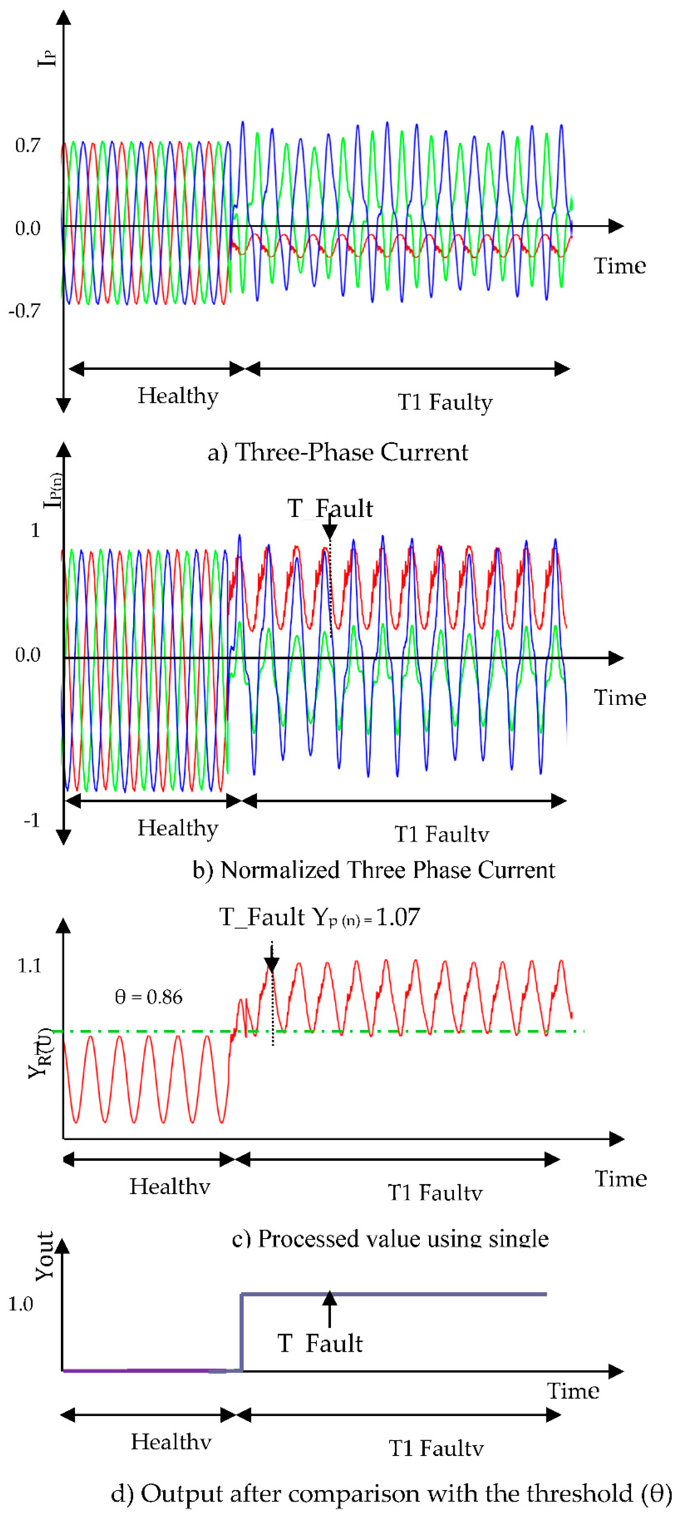
Single switch open-circuit fault (T1):

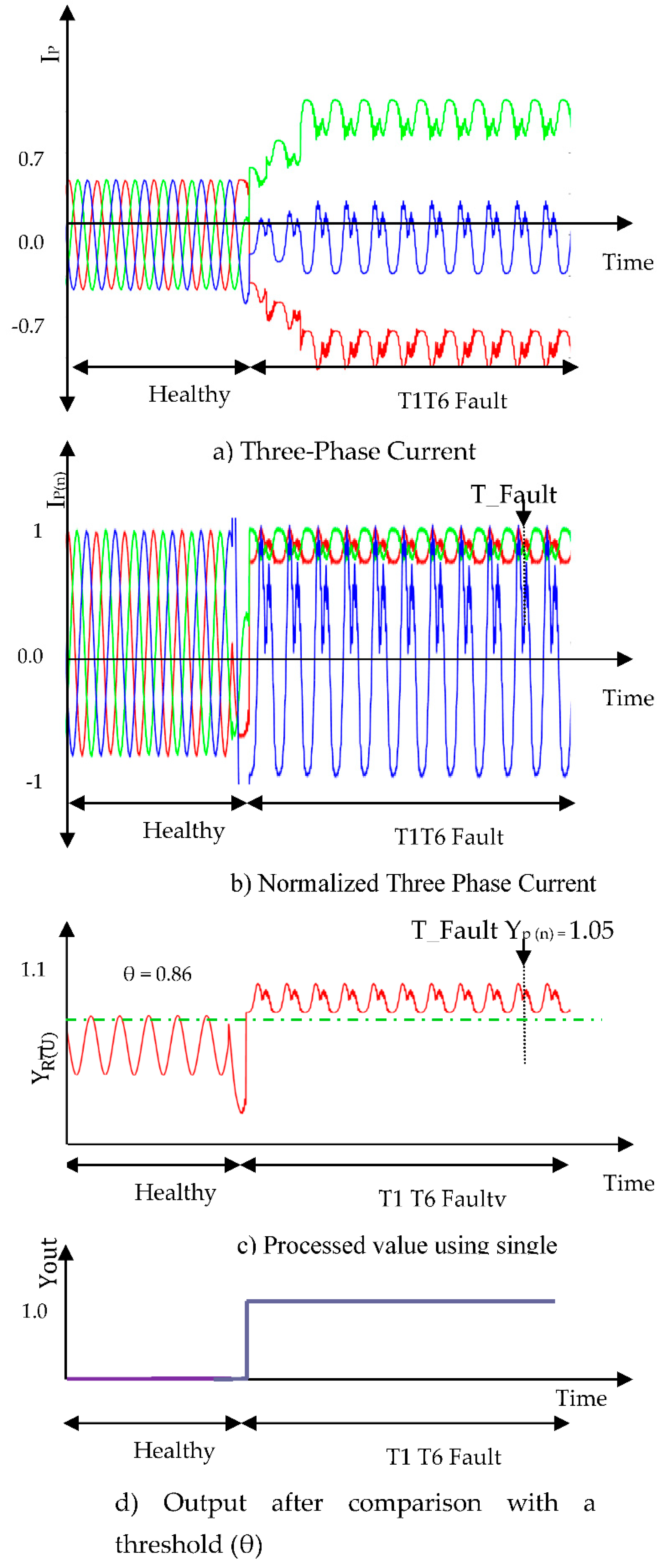
In this, an open circuit fault is generated in T1 at time instant T_Fault. It is required to avoid false interpretation of waveforms of three-phase signals. Hence evaluation of the output is done with the help of processed value. All the waveforms are shown in Figure 3. In this case, a sample value is taken from the normalized three-phase current waveform, R = 0.9162, Y =0. 315, B = 0.8746 giving processed value ${\mathrm{Y}}_{\mathrm{R}\left(\mathrm{U}\right)}$= 1.0727. As the processed value is greater than the threshold value, it indicates that switch T1 is faulty.

B. 

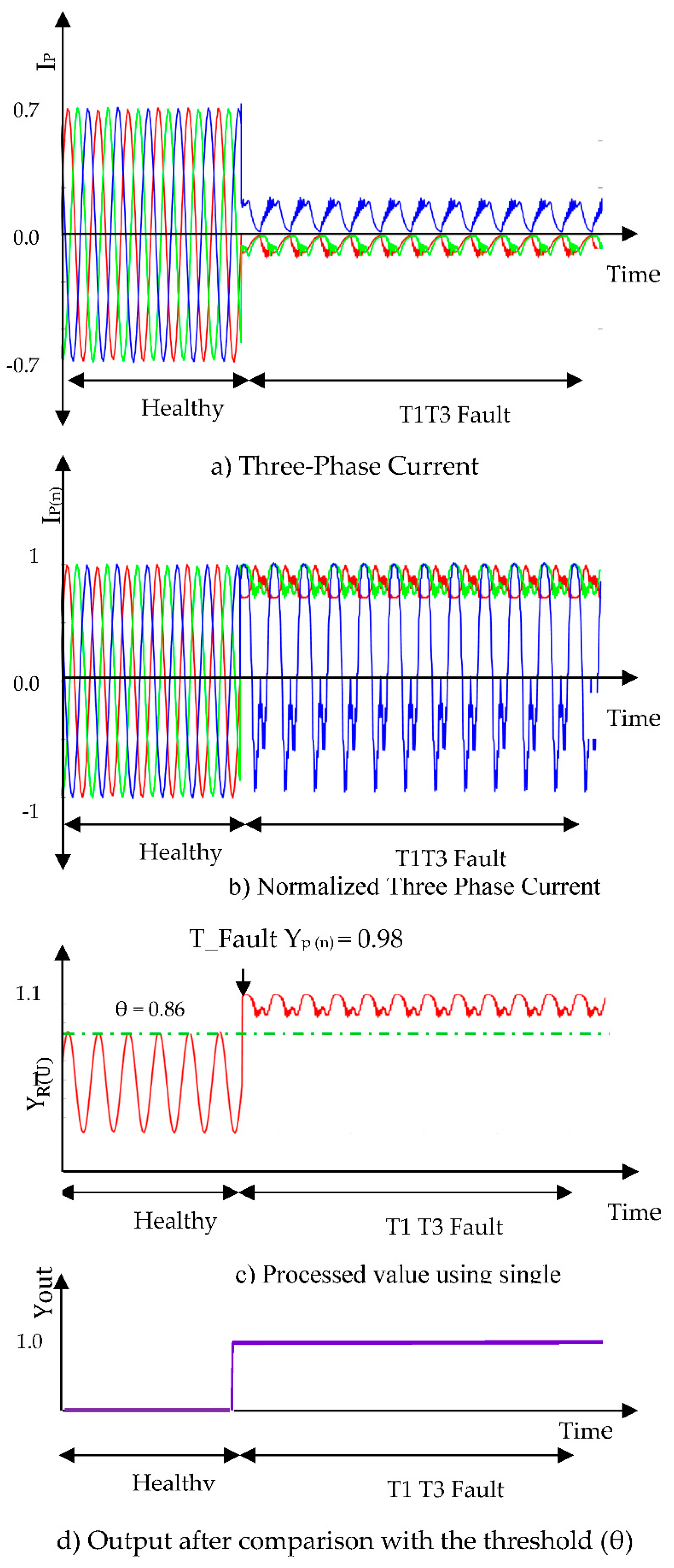
Double switch OCF in the upper part of different legs (T1-T3):

Switches T1 and T3 are present in the upper part of the different legs in an inverter. In an inverter, the fault is introduced in T1 and T3 switches. The time domain waveforms of three-phase current in healthy as well as in faulty conditions at different phases are shown in Figure 4. For analysis purposes sample values from the waveform of Normalized Three-phase current are taken at time instant T_Fault-1 as shown in Figure 4.b, R= 0.721, Y= 0.996, B= 0.980. At this point, the processed value for T1 is ${\mathrm{Y}}_{\mathrm{R}\left(\mathrm{U}\right)}$= 1.0436 as shown in Figure 4.c. As this output value is greater than the threshold value, Y_out=1. It indicates transistor T1 is faulty and shown in Figure 4.d. Same analysis is done at time instant T_Fault-2, R= 0.887, Y= 0.7631, B= -0.5125. For this processed value we get, ${\mathrm{Y}}_{\mathrm{R}\left(\mathrm{U}\right)}$= 0.9465. Hence a fault is indicated with Y_out =1.

C. 

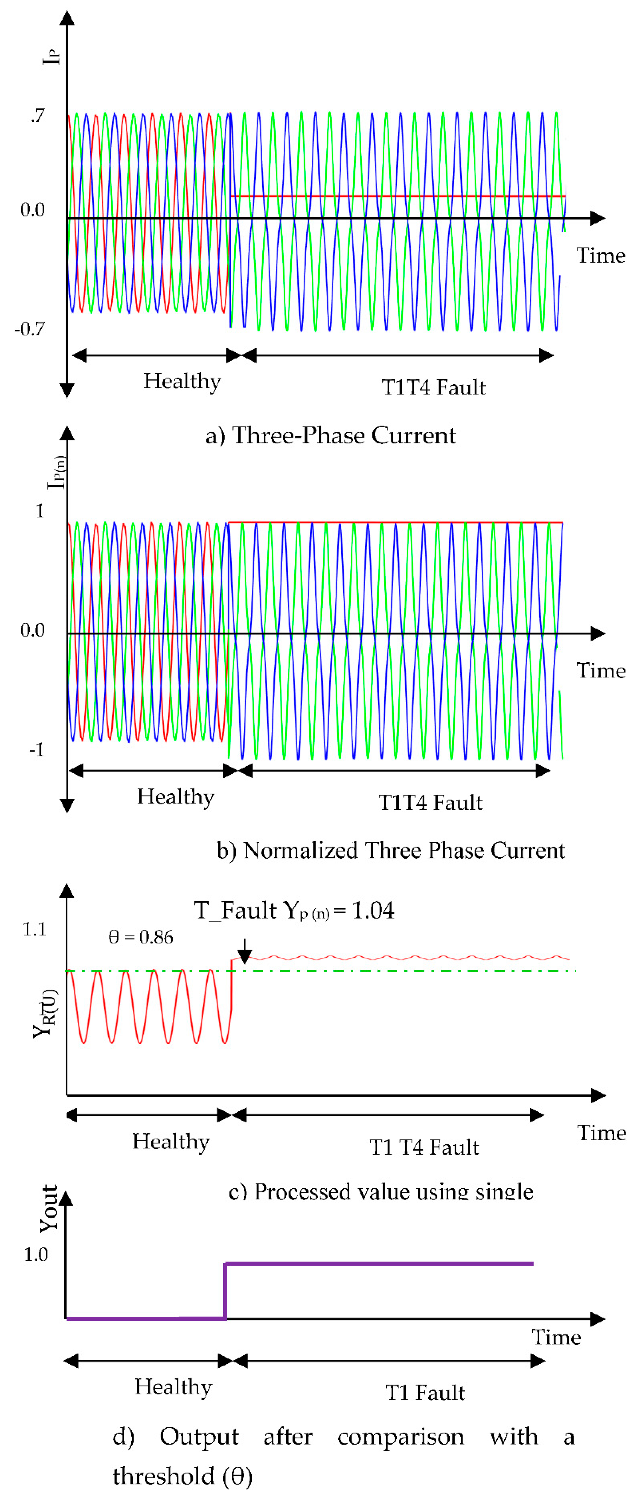
Double switch OCF in the same phase (T1 and T4):

The faults are generated in switches T1 and T4 lay in the same phase. This is a single-phase open fault. The three-phase signal, normalized output, and processed signal waveforms are shown in Figure 5. For the analysis, a sample value is taken from the normalized three-phase current waveform at time instant T_Fault-1 as shown in Figure 5.b, R = 1.0014, Y = -1.1556, B = 0.9881. For this sample, we get ${\mathrm{Y}}_{\mathrm{R}\left(\mathrm{U}\right)}$ = 0.9228, which indicates transistors T1 is faulty as shown in Figure 5.c. The same procedure is repeated for R = 0.8248, Y = 0.3526, B = 0.9648 giving processed value ${\mathrm{Y}}_{\mathrm{R}\left(\mathrm{U}\right)}$ = 1.0149. This shows that switch T1 is defective.

D. 

Double switch OCF in different legs (T1 and T6):

In this, an open circuit fault is generated in T1 and T6 at time instant T_Fault. All the waveforms are shown in Figure 6. In this case, a sample value is taken from the normalized three-phase current waveform, R = 0.9162, Y = 0.8746, B = 0. 315 giving processed value output= 1.0599. As the processed value is greater than the threshold value, it indicates switch T1 is faulty.

E. 

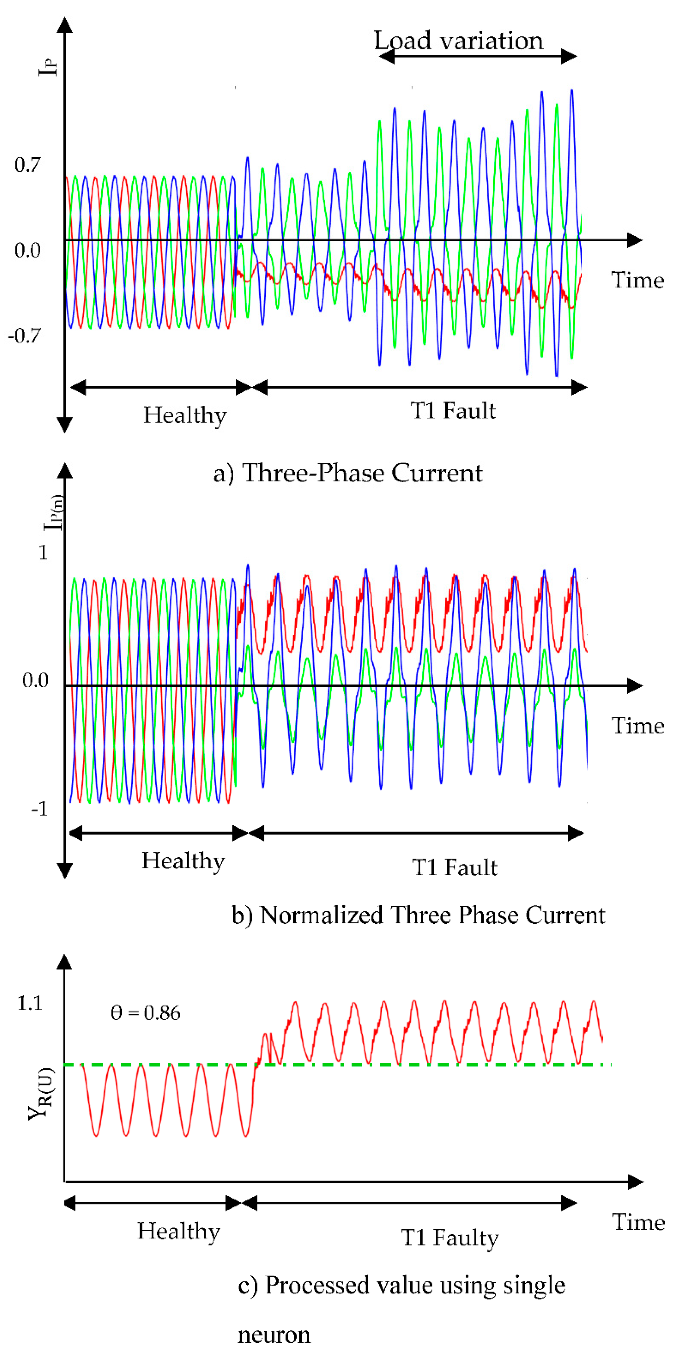
OCF diagnosis under variable load conditions:

The time domain waveform of transient caused due to load variation from light to heavy load during T-1 fault condition is shown in Figure 7.a. Due to load variation, the amplitude of three-phase voltage is changed and generates variations in sensed three-phase voltage. Three phase currents are normalized in the range of ±1 shown in Figure 7.b. An unimportant change in the amplitude is observed in load voltage during load variation, which is no sudden rise or fall in the current signal. Hence, the results of HISNA will not affect. The values of ${\mathrm{Y}}_{\mathrm{R}\left(\mathrm{U}\right)}$after IGBT fault are very high as compared to the values of threshold as shown in Figure 7.c.

A comparison of various open switch fault diagnosis methods based on their effectiveness, resistivity, detection time, implementation effort, tuning effort, diagnostic capability and threshold dependence is given in Table 3. The Park’s Vector method shows ambiguity at small currents and has poor resistivity under such conditions, with a detection time of 20 ms. It requires medium implementation effort and high tuning effort but is limited to diagnosing single switch faults with high threshold dependence. The Slope method also struggles at small currents, with poor resistivity and a higher detection time of 38.3 ms. It has low implementation effort but high tuning effort, diagnosing only single switch faults with high threshold dependence. The Centroid-based fault detection method demonstrates good effectiveness and resistivity but lacks reported detection time and tuning effort. It is capable of diagnosing single switch faults without a specified threshold dependence. The Wavelet-Fuzzy method performs well if fuzzy rules are carefully designed, showing good resistivity and a detection time of five cycles. However, it requires high implementation effort and medium tuning effort, with low threshold dependence. The Wavelet-Neural Network approach achieves a diagnosis error of less than 5%, with good resistivity if the neural network is thoroughly trained. While its detection time is not specified, it demands high implementation effort due to neural network training but requires low tuning effort. It is capable of diagnosing double switch faults without threshold dependence. The Modeled-Based ANN method exhibits a prediction rate of around 75% but has unspecified resistivity, detection time, and tuning effort. It requires high implementation effort and is capable of diagnosing double switch faults. The Hybrid Approach, which combines Park’s Vector and Wavelet-Neural Network methods, offers good effectiveness and resistivity with a significantly reduced detection time of ¼ cycle. It requires high implementation effort and can diagnose multiple switch faults without threshold dependence. The proposed HISNA system demonstrates similar advantages, achieving good effectiveness and resistivity with a detection time of a cycle. However, it requires lower implementation effort compared to the hybrid approach while maintaining the capability to diagnose multiple switch faults without threshold dependence.

Figure 2. B. Circuit diagram of fault diagnosis method.

Figure 2. B. Circuit diagram of fault diagnosis method.

Figure 3. Results regarding the time-domain waveforms of the three-phase currents, the normalized currents, ANN processed output, and the diagnosis result of T1 open circuit fault.

Figure 3. Results regarding the time-domain waveforms of the three-phase currents, the normalized currents, ANN processed output, and the diagnosis result of T1 open circuit fault.

Figure 4. Results regarding the time-domain waveforms of the three-phase currents, the normalized currents, ANN processed output, and the diagnosis result of T1-T3 open circuit fault.

Figure 4. Results regarding the time-domain waveforms of the three-phase currents, the normalized currents, ANN processed output, and the diagnosis result of T1-T3 open circuit fault.

Figure 5. Results regarding the time-domain waveforms of the three-phase currents, the normalized currents, ANN processed output, and the diagnosis result of T1-T4 open circuit fault.

Figure 5. Results regarding the time-domain waveforms of the three-phase currents, the normalized currents, ANN processed output, and the diagnosis result of T1-T4 open circuit fault.

Figure 6. Results regarding the time-domain waveforms of the three-phase currents, the normalized currents, ANN processed output, and the diagnosis result of T1T6 open circuit fault.

Figure 6. Results regarding the time-domain waveforms of the three-phase currents, the normalized currents, ANN processed output, and the diagnosis result of T1T6 open circuit fault.

Figure 7. Results regarding the time-domain waveforms of the three-phase currents, the normalized currents, ANN processed output and the diagnosis result of T1 open circuit fault under variable load conditions.

Figure 7. Results regarding the time-domain waveforms of the three-phase currents, the normalized currents, ANN processed output and the diagnosis result of T1 open circuit fault under variable load conditions.

5. Conclusion

In this work, a single neuron is constructed using basic electronics components. The delta learning rule has been used to find the values of the weights and biases. Using this algorithm, three weights and one bias are calculated for each switching device. The current signal is converted into voltages using a V-I converter. Normalized three-phase voltages are given as input to a single neuron model. The paper explains how all the training samples needed to train a single neuron were collected. The built-in single neuron model was tested with all combinations of switching devices like single switch faults, double switch faults in the same leg, and double switch faults in different legs. The proposed HISNA system outperforms existing open switch fault diagnosis methods by offering good effectiveness and resistivity with a fast detection time. Unlike the Hybrid Approach, which requires high implementation effort, HISNA achieves similar diagnostic accuracy with lower effort. Traditional methods like Park’s Vector and Slope suffer from poor resistivity and longer detection times, while ANN-based techniques demand intensive training. HISNA ensures efficient multiple switch fault diagnosis without threshold dependence.