
Submitted:
23 November 2024
Posted:
25 November 2024
You are already at the latest version
Abstract
Recently, fault detection has proven its crucial role in guaranteeing the safety and dependability of inverter functioning. This paper demonstrates the effectiveness of employing Artificial Intelligence (AI) approaches for fault detection of single Open Circuit (OC) switch fault in a Packed E-Cell (PEC) inverter. Two optimum strategies have been considered Random Forest Decision Tree (RFDT) and Feedforward Neural Network (FFNN). Initially, Discrete Wavelet Analysis (DWA) is employed for the investigation of the output voltage, using the first level of detailed coefficients. After that, three statistical features are extracted from this analysis to serve as input to the classifier during learning. The output of the classifier, which is referred to the fault class, is then trained according to each strategy process. Finally, a comparison with deep analysis based on selected criteria is illustrated and the results obtained using MATLAB/Simulink confirm the comprehensive review of the evaluated strategies.
Keywords:
Wavelet Analysis
; Feature Extraction
; Switching Faults
; Random Forest Decision Tree
; Feedforward Neural Network
; Fault Detection
1. Introduction
Countries are investigating innovative techniques of electricity generation due to the constraints of energy supplies. In addition to the shortage of fossil fuels, conventional electrical generation challenges environmental problems which thereby make energy from renewable sources grow progressively. Given that Photovoltaic (PV) energy generation is free of contaminants, safe, noiseless, and absolutely free it has drawn a lot of concern in the context of sustainable power transformation. Grid-connected PV systems are evolving rapidly than standalone PV systems. PV panels operate in two stages: first, the PV array converts solar energy into a continuous voltage, and then by means of an electronic device called an inverter, the continuous voltage is converted into a sinusoidal voltage to be utilized by the power grid. For maintaining the precision of PV systems operation, the reliability of inverters is crucial.
Although both PV arrays and inverters are susceptible to malfunctions, PV arrays are guaranteed to endure for over 20 years, yet inverters have a typical free of errors lifespan of barely two years. Initially two-level voltage has been produced using conventional two-level inverters, creating a quasi-square wave. In 1975, multilevel inverters (MLI) had been developed in industry to generate high-voltage sinusoidal waves that have the potential to be linked to the electrical grid. Nevertheless, these inverters involve an extensive number of switches, which raises their degree of complexity and expense. Furthermore, the likelihood of switch failures has increased where Studies conducted on more than 200 industrial items from 80 industries indicate that inverter faults are typically triggered by defects in capacitors and device-module. Faults in capacitor account for 30% while faults in device-module account 60% of all failures in a converter system of which 21% of faults exist in semi-conductors, 13% in solders and 26% in printed circuit board [1].
Faults in capacitors arises slowly, initially as an alteration in functioning that can be detected before the final malfunctioning. Therefore, early identification is achievable and identification is not complicated. Therefore, studies are currently focusing on faults in power semiconductor switches, which, if not recognized, could result in disastrous consequences. Switch Failures are primarily categorized into OC faults, short-circuit faults, and freewheeling diode OC faults. The latter are uncommon in multi-level inverters because they are caused by diode reverse-recovery breakdowns and external breaking between power semiconductor modules and electrical load problems. The most typical and dangerous breakdown condition in MLI is switch short circuit fault, as it results from either a continuous gate signal caused by defect in a drive or control circuit or from an unusual rise in temperature caused by overvoltage or overcurrent leaking. Unfortunately, not only short circuit failure results in instantaneous breakdown of the system but also removing it is considered extremely challenging. Consequently, electronic safety systems including relays, fuses, and circuit breakers are frequently employed [2]. On the other hand, OC failures can be attributed to a various issue, such as failure of the gate signal, internal connection failure from overheating, bond wire lift-off from thermal cycles, and interruption in external connections from disturbances. Even though OC faults result in less dangerous effects than short circuit faults because they do not cause system closure yet prolonging the system's functioning in the instance of an OC fault can end up in fault enlargement, which will eventually lead to breakdown in related components, lowering electricity capacity, pulsating currents, and increasing distortion in harmonics, leading to the shutdown of the system and higher repair costs [3].
Hence, to ensure continuous functionality of MLI, extensive research has been carried out regarding the recognition and evaluation of OC failures. OC fault detection approaches for different multilevel inverter architectures have been extensively studied by researchers. These methods can be divided into two primary groups: hardware-based and system-based. Hardware-based methods, which mostly use sensors to gate drivers, offer quick identification yet they can frequently lead to additional complications, bigger system dimensions, and repair expenses. Researchers have therefore thoroughly examined system-based diagnosis methods for identifying switch defects that depend on an investigation of voltage and current waveforms. These methods fall into three main categories: algorithmic, signal processing and model-based strategies. The latter optimally intent to exclude the usage of current/voltage sensors, thereby it relies on existing models that utilize numerical functions to establish interactions among system inputs and outputs. They are carried out through residual production and residual assessment. Even though model-based methods are distinguished by their superior performance in the context of transient systems, they nevertheless possess certain drawbacks. Initially these techniques depend strongly on model accuracy, in which any modification in the model's factors or its variables will affect the preciseness of the identification. Furthermore, the primary difficulty with these approaches is choosing appropriate thresholds [4,5,6]. Additionally, these techniques require a time delay in order to prevent false alarms produced by noise, which significantly slows down the method of identification [7,8,9,10].
Using signal processing techniques, an extensive and comprehensive analysis of OC switch failure detection in various multilevel inverter topologies is illustrated in [11]. Abnormal deviations in the signals are observed whenever an OC fault occurs in a switch, yielding fault data that prompted researchers to carry out mathematical or analytical procedures on the observations. These strategies can be broadly divided into voltage-based and current-based techniques. It is widely acknowledged that variations in load can affect the output current generated, which could lead to incorrect categorization. However, output voltage remains unaffected by variations in load, so employing it as a defect detection function is more efficient. The following categories are further classified into voltage- based diagnosis strategy, current - based diagnosis strategy, multisource - based diagnosis strategy and time – frequency domain analysis.
Despite the fact that signal processing techniques don't require sophisticated learning and training or a mathematical model, they possess a limited awareness of the operational input signals, which means that unexpected incoming disturbances could compromise the system's reliability [12]. Additionally, the majority of these technologies' applications demand extra detectors. Time delay is also an important factor to take into account while constructing a system. However, techniques based on voltage signals are less influenced by fluctuations in frequency and provide quick failure identification. Nevertheless, they should be modified to improve system dependability to be applied on recent inverters. Further, referring to current waveform-based procedures, a number of diagnosis techniques that depend on current waveform analysis might not operate correctly if the device has on-load-side OC faults since these defects interrupt the continuation of the current output. Unfortunately, this restriction has not been examined or studied in further detail by existing inverter OC fault detection techniques.
In contrast to model-based and signal-based approaches, the technique of AI uses previously collected information to recognize the correlation between the retrieved attributes based on the operation circumstances, eliminating the need to set thresholds along with building exact numerical models [13,14,15,16]. Expert expertise is used in AI algorithm diagnostic approaches to improve knowledge library excluding mathematical models or sensors. Once it relates to demonstrating smart theory, one ought to first review the knowledge library which matches with the failure state that will be subsequent to failure diagnosis. Nonetheless, the process of gathering information leads to the creation of the defect data library. As a result, this category will have a less durable performance and increased efficiency. Thus, emphasis is placed on failure detection relying on AI algorithms, extensively studied in [17], due to their potent functionality, enhanced efficiency, and excellent potential for self-learning.
This paper demonstrates a comparison between ML using the RFDT strategy and Deep learning using FFNN for fault detection of single OC switch fault. Initially, a brief description of the PEC inverter topology under study, its circuit and modulation is fully explained. Then, the implemented fault detection algorithm is established. Further, the methodology is outlined concerning data preparation, model descriptions, training and testing process. Next, metrics used to evaluate the models is presented. Furthermore, the simulation results along with comparison and discussion are fully discussed. Finally, the paper concludes with a summary of the findings.
2. PEC Inverter Topology and Modulation Technique
MLI are essential to grid-powered electrical systems considering their minimal total distortion of harmonics, flexible structure, and need for fewer filters. Therefore, a new advancement in multilevel inverters referred to as compact units—has popped out to get over the drawbacks of the conventional multilevel topologies. In comparison with regular configurations, these compact units rely on "reduced-structure" architectures, that employ lesser active and passive constituents. As seen in Figure 1, an innovative PEC single-source inverter was introduced in 2019 to provide a nine-level output voltage [18].
Through this layout, the capacitors are arranged horizontally and an extra DC-link is built to guarantee a balanced voltage across the capacitors. Using signal building modules, a unique technique described in [19] controls the switching states required to generate the nine-level signal while preserving same voltage across the capacitors. Two signal builders—one for charging the capacitors and the other for discharging them alternately regulate the DC-link voltage till the Vdc-link voltage approaches fifty percent of the DC source voltage, with the voltage capacitors being maintained at twenty-five percent of the DC source voltage. The efficient operation and excellent performance of the MATLAB Simulink simulation outcomes convey as validation for this. A nine-level voltage signal is produced using simple modulation and a shorter computation time after having capacitor voltage balancing.
3. Fault Detection Strategy
Figure 2 shows a flow chart that illustrates the suggested fault detection approach. The voltage that emerges from the output at the load is created on behalf of running of the multilevel inverter. A wavelet transform is then used to derive features, and statistical indicators are then calculated. These features are used as input labels for the classifier model and the switch number associated with the failure is considered the output label. Eventually, using the loading-trained model, estimation and identification of faults are accomplished. Hence, the three primary steps including data processing and preparation, neural network training, and network evaluation criteria—are described fully below.
4. Methodology
4.1. Data Preparation and Processing
4.1.1. Data Generation
Once an electrical switch encounters an OC failure, it causes unanticipated deformities in the voltage and current signals. Yet since the generated current is impacted by load modifications, that can result in incorrect categorization, depending on the produced output voltage is a more trustworthy characteristic for detecting defects considering that it 3remains uninfluenced by fluctuations in load. As demonstrated in Figure 3, this study investigates 24 different load levels, with each load consisting of eight no-fault states and one with a single defective switch. Each state's output voltage is recorded, yielding 192 dataset points.
4.1.2. Wavelet Transform
Using the wavelet transform, a signal can be broken down into its frequency components. Wavelet transforms can be divided into two primary categories: DWT and continuous wavelet transform. The latter tool offers a comprehensive depiction of waveforms. On the other hand, DWT divides signals into groups. The DWT is especially well-suited for tasks as feature extraction, compression, denoising, and examining the statistical properties of wavelet coefficients. Both approximation and detailed coefficients are obtained during wavelet decomposition. The detailed coefficients preserve thinner, high-frequency information, whereas the approximate coefficients provide a larger, smoothed representation of the data [20,21,22,23,24]. This study uses the Daubechies wavelet "db4" to perform a detailed coefficient for the voltage at the output. In particular, only one level of decomposition is used, deriving the primary set of detail coefficients.
4.1.3. Feature Selection
Mean and standard deviation are extensively used as statistical metrics in basic linear analysis of information. Nevertheless, its dependability suffers whenever tackling application scenarios that are which include inequality and extremists. As a result, skewness and kurtosis, which describe absence of symmetry and the extent of outliers, are better statistical metrics for frequency analysis of information. For example, in articles [25,26,27,28], researchers proved the usefulness of using kurtosis and skewness for recognizing defects, providing results from simulations demonstrating feasible and reliable fault identification.
The feature selection approach employed is determined by the dataset's specific characteristics as well as the study' aims. Evaluating the dataset and choosing a suitable feature selection strategy based on its properties is critical. There are several ways for picking characteristics, each having advantages and disadvantages. Initially, the filtering method assesses each characteristic independently and picks the most significant aspects using statistical metrics such as correlation and shared knowledge. Filtering algorithms are fast and straightforward to construct; however, they may not take into account relationships between features and may be ineffective with large datasets. In contrast, the wrapper technique employs an algorithm for learning to assess the utility of each portion of the functions. Wrapper techniques are considerably more computationally costly compared to filter techniques but they take into account relationship between features and may perform better in datasets with large dimensions. However, they are more susceptible to excess fitting and may be affected by the learning method used. Random Forest Elimination (RFE) has a distinct advantage over filter and wrapper approaches due to the fact that it takes into account the significance, redundant operation, and relationship between features. RFE can successfully decrease the overall size of an information set by iteratively deleting the least significant features while retaining those with the greatest informative characteristics. Nevertheless, RFE can be computationally demanding, making it inappropriate for huge datasets. Nonetheless, Principal Component Analysis (PCA) converts attributes into a space with little dimension that contains the most relevant information. PCA is an excellent method for reducing the overall size of information and eliminating duplicate features. However, it could lose the understanding of the original features and may not be appropriate for non-linear correlations between attributes. Thus, RFE highlights the most important elements that are crucial to a classification model's prediction ability. RFE with a predetermined number of features to pick is used. This technique creates a model utilizing the rest of the attributes after repeatedly discarding part of the features, depending on model accuracy to identify which features are particularly relevant in forecasting the target feature. For example, researchers in [29,30] used the RFE method to pick a meaningful and crucial set of characteristics, resulting in appropriate classification. As a result, numerous iterations with varying numbers of features chosen are performed, and the accuracy of each iteration is captured, allowing for an examination to determine how choosing features affected the model's efficiency throughout iterations. Simulation findings demonstrate that selecting three or four features produces a similar average accuracy of 65%. However, as seen in Figure 4, using three aspects led to greater accuracy in some cases than utilizing four features. Thus, standard deviation, skewness, and kurtosis are regarded as significant.
4.1.4. Data Augmentation
Data augmentation is the process of intentionally producing fresh data for training by either using novel fabricated data generated from existing information or inserting substantially altered duplicates of existing dataset. This method improves accuracy, minimizes overfitting, and increases the model's generalization power, which leads to considerably more reliable machine learning models [31,32]. At first, establish parameters such as the quantity of samples to match to the size of the features. Then, set the augmentation factor, which is adjusted to 2 to twice the dataset as needed, as well as the appropriate noise level of 0.05. Then, create a noisy version of the features where firstly noise is calculated by applying this equation
noise = noise_level * randn(num_samples)
Assuming 3 features (Standard, Skewness, and Kurtosis) and then getting updating features in which:
Noisy_features = features{:,:} + noise
Thus, the feature data for each state are tripled from 24 to 72, resulting in a total of 576 dataset points.
4.1.5. Minimum Max Normalization
Normalization is a scaling method in Machine Learning that is used during data collection to adjust the numbers of numeric columns in the dataset so that they utilize the same scale. It is not required for each dataset in a model. It is only necessary when the features of machine learning models have distinct ranges. Though there are various feature normalization approaches in Machine Learning, Min-Max Scaling method is used in this paper. Applying this technique, the dataset is shifted and rescaled to end up ranging between 0 and 1 using this equation:
Xn=(X-Xmin)/(Xmax-X min)
In which Xn = Value of Normalization; Mmaximum = Maximum value of a feature; Xminimum = Minimum value of a feature
- Case 1: If the value of X is minimum, the value of Numerator will be 0; hence Normalization will also be 0.
- Case 2: If the value of X is maximum, then the value of the numerator is equal to the denominator; hence normalization will be 1.
- Case 3: On the other hand, if the value of X is neither maximum nor minimum, then values of normalization will also be between 0 and 1.
4.2. Model Descriptions
4.2.1. RFDT Strategy
This group refers to supervised machine learning techniques that employ sequential graphs. Its primary idea is to use basic decision rules which can be learned from training data to predict the class of the target variable. To get the ultimate decision, each possible outcome is considered from top to bottom. The DT approach has demonstrated superior results in the diagnosis of OC switch faults [33] considering its optimal accuracy, robustness, and quick identification period of time.
To produce accurate estimations, increase accuracy, and lessen overlapping, the RF approach remotely builds several DT and aggregates the estimates in a similar way. Additionally, it employs random sampling by employing distinct data sets during the tree-building process and choosing features for each tree randomly. The retrieved voltage signal was used as input for training a number of machine learning algorithms in the [34], and optimum key matrices were used to assess each algorithm's functionality. The effectiveness of the RFDT classifier has been confirmed by simulation results, which show that it can accurately and robustly identify faulty switches. Figure 5 demonstrates the architecture of RFDT model having multiple decision trees each having different dataset group to get final result based on weighted average voting.
4.2.2. FFNN Strategy
Initially, Figure 6 shows the 3D data representation of the chosen features. As can be seen, multiple faults exhibit similar values for these features as they overlap and cannot be easily separated. Actually, not every type of machine learning is deep learning, even though all deep learning involves machine learning. Neural networks with multiple layers, thus named as deep, are used in deep learning as a specifically designed subset of machine learning for analyzing complicated structures in data. Notably, both supervised and unsupervised learning can be used in deep learning. The first step involves feeding the algorithm a paired dataset that consists of a sample and its label. These inputs are also known as instances or findings to be classified. The algorithm, on the other hand, operates in an unsupervised way whenever datasets are not labelled in which output categorization, computation, and implementation is carried out in the absence of previously defined features.
Despite the fact that unsupervised learning is more effective in finding novel patterns and connections in unlabeled, raw data, nevertheless a number of obstacles still exit. A number of unsupervised intelligence techniques have been applied to the data gathered from the inverter that is being studied. Unfortunately, employing Gaussian Mixture Models, which calculate the likelihood that a given data point belongs to a cluster, or Autoencoders with Clustering or Self Organizing Maps, which re-represent high dimensional points in a reduced dimensional region have resulted in inadequate results. Thus, supervised deep learning neural networks were the main focus of this paper.
Numerous unsupervised structures for deep learning have been addressed in studies, where according to data type each architecture is applied. For example, Recurrent Neural Network, Long Short-Term Memory, and Gated Recurrent Unit networks work well for time-varying and consecutive data types [36,37,38,39,40,41] whereas Convolutional Neural Networks are frequently employed for image-based or geographical data, particularly when combined with spectrograms or thermal images [42,43,44,45,46,47]. On the other hand, Deep Belief Networks and Deep Fully Linked Networks are appropriate for large scale or complicated feature structures [48,49,50]. Hence, FFNN and Back Propagation Neural Network (BPNN) are the two most commonly used varieties. Within the FFNN type, the input array proceeds via the first layer, whose output values constitute the input vector for the following layer. Similarly, the output of the preceding layer generates the input vector of the layer that comes after. This process repeats up until the network outputs the results of the last layer; the more layers there are, the more deeply the data gets learned to reveal complicated patterns and correlations. For instance, in order to identify OC switch faults for cascaded H-Bridge MLI, the authors in [51] implemented an Artificial Neural Network (ANN) based on FFNN type after using a feature extraction procedure by multi resolution wavelet analysis. However, there are two primary operations in the BPNN category which are forwarding propagation of signals and back propagation of errors. The training feed forward network can be expanded in reverse, having error computation functioning as the basic principle of BPNN. Initially, the difference between the actual and predicted amounts by the network is calculated. The goal is to reduce the neural network error by recalculating the weight values in each layer, starting with the last and working backwards to the first layer. Additionally, the gradient descent approach is used to train BPNN in order to modify the neural network's weight where authors in literature have provided several examples of fault diagnosis for OC switches by choosing voltage characteristics for BPNN training [52,53]. Unfortunately, BPNN has a weakness in that it has a slow convergence time and quickly collapses into a local minimum level. As a result, feed forward NN is used due to its easy implementation and efficient training.
A FFNN is a type of ANN where connections between nodes do not form cycles. In simple terms, the data flows in one direction, from input to output. Figure 7 depicts the structure of the neural network designed for detecting and diagnosing faults in inverters. Figure 8 depicts the structure of the neural network designed for detecting and diagnosing faults in inverters. The architecture of our neural network consists of an input layer comprising three feature inputs as mentioned earlier, hidden layers comprising certain number of neurons to be specified later and an output layer comprising eight predictable outputs corresponding to the number of switch defects and no-fault case. The main idea of the Neural network is creating predictions in accordance to the current weights and biases following these steps:
- Input Layers: The input layer receives the scaled data that has been retrieved. After that, weights are employed as the data is transmitted through each hidden layer.
- Hidden Layers: After executing multiple simulations using various transfer functions in hidden layers, the activation function for hidden layers in this paper is set to 'tansig', a hyperbolic tangent sigmoid function required for establishing uncertainty at every single layer and to identify the output of each neuron.
- Output Layer: The network's estimate is provided by the output layer once the information that was analyzed has been delivered.
4.3. Training and Testing Process
Training a classifier, assessing its effectiveness, and storing the model for the detection stage are the main objectives of this section. First, the scaled dataset is uploaded, and the grp2idx function is used to transform the categorical labels to numeric labels for additional analysis. The data only in FFNN method is then shuffled to create random indices for splitting. Then, the data is subsequently divided into two sets: 70% for training and 30% for validation.
4.3.1. RFDT Model
The template Tree with these parameters ('MaxNumSplits', 50, 'SplitCriterion', 'twoing', 'Surrogate', 'on', 'MergeLeaves', 'on') with 300 learning cycles is considered for the RF Classifier in which a Gradient Boosting (GB) machine classifier is trained. The number of splits is specified to a certain value to manage the trees deepness thereby minimizing level of complexity. As well as avoiding overlapping. Moreover, the towing criterion focuses on attempting to more clearly divide classes by optimizing the disparity between groups produced by the split which affects the classifier's capability to manage unbalanced or multi-class data. On the other hand, surrogate splits allow each tree to manage missing data more successfully making the model more robust to missing values, in which alternative split features act as stand-ins when necessary. Moreover, “MergeLeaves = on” points out that leaves that do not significantly enhance the final estimate are merged thereby minimizing overlapping. Figure 8 illustrates a flow chart for training RFDT model. Each new tree in the series is trained to resolve the errors that occurred the ones preceding it, with an emphasis on instances from prior trees that were incorrectly classified. The objective is to create trees that gradually decrease errors in order to continuously decrease the loss function. Standard RF bagging (parallel learning), in which every tree is a standalone entity, is not the same as this method of successive learning of trees. GB, on the other hand, concentrates on errors and develops over preceding cycles to create a robust model.
4.3.2. FFNN Model
Regarding the learning process, the Levenberg-Marquardt (LM) algorithm, executed in MATLAB as “trainlm”, is generally considered an effective training technique, particularly for small to medium in size networks since it captures additional information about the error surface. It overcomes the issue caused by rapid convergence through integrating elements of the Gauss-Newton and gradient descent approaches. Combining the advantages of both the Gauss-Newton approach and gradient descent, LM adjusts the weights by resolving a non-linear least-squares issue instead of utilizing basic gradient descent. This requires calculating a Jacobian matrix and applying it to more efficiently modify weights for complicated, non-linear error situations.
For optimal model performance as well as learning effectiveness, a number of conditions are crucial. First, a key factor in the model's effectiveness is the actual number of hidden layers. Narrower networks (1-2 layers) are typically preferable for the dataset used in this article since deeper networks with smaller datasets are more likely to overfit when trained. As a result, the network model employs only two hidden layers. The number of neurons that make up each hidden layer, however, is similarly essential. For a variety of classification problems, hidden layers containing 10–50 neurons are frequently essential for preventing overfitting during training. Additionally, when training neural networks with the LM algorithm, four important parameters should be adjusted to maximize model performance: learning rate, maximum number of training epochs, maximum validation failures, and regularization parameter. Learning speed, convergence stability, and network generalization are all influenced by these characteristics. To begin with, the maximum number of epochs (trainParam.epochs) sets the maximum number of training iterations (epochs) is set as default value of 1000. The number of consecutive validations increases allowable before early stopping is accordingly limited to 50 using the maximum validation failures (trainParam.max_fail) parameter. Additionally, the weight update's step size is controlled by learning rate. Although a reduced learning rate strengthens training but necessitates numerous iterations, an increased learning rate accelerates training process but runs the risk of surpassing the required level of accuracy. As a result, the learning rate range of 1x10⁻⁴ to 1x10⁻¹ is selected. Moreover, the regularization parameter is crucial for creating strong models that adapt effectively to freshly acquired data. Though bigger values (which enforce more weight decay) might lessen overlapping, smaller values have less influence on weights and maintain adaptability. Therefore, the range of regularization parameter between 1x10⁻⁵ and 1x10⁻¹ is selected.
Figure 9 demonstrated the Bayesian optimization process implemented. Initially, the ranges for hyper parameters such as neuron number in each hidden layer, learning rate, and regularization are defined. Then, the optimization procedure iterates to find parameters that minimize validation error. During each iteration, a neural network is trained using the LM algorithm with early stopping to prevent overfitting; if the model’s validation error does not decrease after a number of checks, the training process stops, and the best weights are retained. After that, Bayesian optimization uses the results from each iteration to select new parameters, continuing this loop until reaching the maximum iterations or the lowest validation error. Ultimately, simulation results of this process yield the optimal parameters in which learning rate ana regularization parameter are adjusted to 0.036805 and 0.0096611 respectively thereby leading to the minimum validation error utilizing two hidden layers, the first with 43 neurons, and the second with 46 neurons.
Once the training process ends, the error histogram and performance graph during training and validation resulted in Simulink are presented in Figure 10 and Figure 11 respectively. Error variations for two data sets are shown: training and validation. From the above two figures it is evident that when neural network is adopted for fault detection an error of order 0.05 is achieved in most of the cases as shown in histogram. It is shown that the error decreases considerably at the end of the training process. The total number of iterations for training of neural network is around 231. The error rate is minimized and reaches 2.1632x10⁻² at iteration 181 during validation after which the error starts increasing.
5. Evaluation Performance Metrics
The validation data is passed through the network to get predictions which are converted back to class labels. Then, the accuracy on the validation set is calculated by comparing predicted values with the true labels. However, this is not enough in deep learning systems, thus researchers have proposed specific criteria for evaluating classifier performance as follows:
5.1. Confusion Matrix
In a binary assessment problem, a system of classification assigns a positive or negative rating to events. Combination tables of data, commonly referred to as confusion matrices, are a particular kind of configuration that can illustrate the extent to which a classifier works by offering the arrangement of every result of the prediction and outcomes of a classification issue and contributing in the visualization of its consequences. As seen in Figure 12, a table is displayed showing every classifier's expected and true value. There are four different categories in the confusion matrix:
- True Positive (TP): The frequency at which the real positive values match the expected positive values from the model classifier.
- False Positive (FP): The frequency at which the model classifier incorrectly expects positive values but in reality, it is actually negative i.e., the classifier predicts a positive value, and it is actually negative. It is referred to Type I error.
- True Negative (TN): The frequency at which real negative values match the expected negative values from the model classifier. i.e., the classifier predicts a negative value, and it is actually negative.
- False Negative (FN): frequency at which the model classifier incorrectly predicts negative values but it’s in reality positives i.e., the classifier predicts a negative value, and it is actually positive. It is referred to Type II error.
A deeper understanding of the model's recall, accuracy, precision, and entire efficacy in fault classification is made possible by these predictions.
- Accuracy: The model's accuracy is utilized to assess its performance. It can be expressed as the proportion of all true incidents to all occurrences.Accuracy=(TP+TN)/(TP+TN+FP+FN)
- Precision: The correctness of the model's positive expectations is determined by its precision. It is expressed as the proportion of TP cases to all of the model's true and false positive expected cases.Precision=TP/(TP+FP)
- Recall: A classifier model's recall determines the extent to which it can locate each significant occurrence throughout a dataset. It is the proportion of TP cases to the total of FN and TP cases.Recall=TP/(TP+FN)
5.2. Receiver Operator Characteristic (ROC)
It is an additional instrument used to visually assess a classification model's operation. This is made through showing the extent the number of accurately determined positive cases varies with the number of inaccurately categorized negative instances. Plotting the TP rate, sometimes referred to as recall or sensitivity, against the FP rate at various threshold levels is what the ROC curve does.
5.3. Precision-Recall (PR)
It is additional visual representations of a classification model's effectiveness at various thresholds. The PR curve demonstrates the degree to which a predictive model effectively combines precision and detects throughout different decision thresholds by illustrating precision versus recall values.
5.4. Log Loss
A measurement of the extent to how model's probability prediction’s function is called log loss, also known as cross-entropy loss. By calculating the difference between the predicted and real probabilities, it examines how well the real group classifications fit the expected ones. It can be conceptualized as the negative log-likelihood of the current labels considering the predicted probabilities.
6. Simulation Results & Discussion
After finishing the training of the two classifier models, each model is tested using confusion matrix, PR, ROC, and log loss value. To begin with, in Table 1, accuracy is calculated for each RFDT and FFNN model having 93 and 90 respectively indicating great performance for both models. This indicates high operation for both classifiers. To study the models ‘performance deeply, the calculated log loss value is considered having 0.72 for FFNN model which is greater than 0.47 for RFDT model. The lesser is the log-loss value, the less the predicted probability diverges from the actual value thereby indicating improved performance of RFDT Model. This difference is more clarified through analyzing ROC and PR curves for RFDT and FFNN models below.
Furthermore, Table 2 shows the confusion matrix for the two examined models. The most essential factor in the confusion matrix is the diagonal elements illustrating the truly predicted samples. For example, a total of 160 samples for the RDFT model and 155 for the FFNN model were correctly predicted out of the total 172 samples and 173 samples respectively.
Figure 13 demonstrates ROC curves of the trained classifiers FFNN model and RFDT model. As mentioned above, ROC illustrates the degree to which the total count of correctly identified positive examples fluctuates in relation to the quantity of incorrectly classified negative cases. The ROC curve having upper left corner is the most appropriate location. This demonstrates that the model minimizes false positives while effectively recognizing positive cases. As a result, increasing FPR and moving towards the right side of the ROC plot typically denotes deteriorating functionality of the model as the number of false positives rises. For most classes, the two curves remain close to the upper left, signifying a high TP rate and a low FP rate. In general, this signifies that both models accomplish a good job of differentiating each category. In contrast to the FFNN graph, the RFDT ROC curve appears to be even more concentrated on the left side of the figure, resulting in a marginally lower FPR across the majority of classes which reflects a preferable result. This behavior could point to a general enhancement in minimizing false positives. The fault detection model RFDT might additionally manage all categories with greater consistency, as it seems to operate more regularly across classes with minor variances. Conversely, some classes exhibit a bit more fluctuation in the FFNN graph, with minor decreases in TPR or increases in FPR for particular classes.
Despite the fact that the ROC curve may present an excessively optimistic picture of the model's performance, the PR curve more accurately depicts the effectiveness of the positive class in particular. The accuracy of the model's positive predictions is determined by precision in which high precision points out that model gives true positive values more than false positive ones (few FP). On the other hand, recall establishes how well a model can identify each faulty state in a dataset in which high recall points (few FN). Regarding the overall curve forming illustrated in Figure 14. Graph Showing PR Curve of (a) Trained Classifier FFNN Model; (b) RFDT Model, although the FNN model begins with decreased precision at decreased recall values, it still reaches high precision value as recall value ascends. Nonetheless, the RFDT model typically performs with greater consistency across fault classes, preserving good precision over a broader variety of recall levels. Compared to the FFNN curves, the majority of fault classes in the RFDT curves accomplish precision levels (near 1) throughout a greater portion of the recall spectrum. This implies that RFDT could operate more uniformly across fault types. The FFNN may be less reliable at managing any failure type efficiently because its precision fluctuates considerably across faulty categories according to various recall values. Most faulty categories are increasingly getting close to a recall of 1, indicating that both models have strong recall capability. As seen in figures above as recall values are closer to 1, the RFDT model tends to maintain greater precision value whereas the FFNN model's precision sharply declines in some faulty categories. Therefore, it indicates that the RFDT functions significantly when it comes to preserving excellent recall as well as excellent precision levels throughout faulty categories.
It is worth to mention that training FFNN have taken more time than RFDT which make it computationally expensive. Moreover, it requires tuning a large number of parameters. On the contrary, Random forests are faster to train compared to large neural networks, as each decision tree can be built independently. Training complexity scales with the number of trees, but the method is still computationally more efficient than most neural networks. Although FFNN could be enhanced by increasing number of hidden layers, their learning would be time consuming and advanced hardware equipment is required. To sum up, the RFDT model seems to operate more consistently, thereby rendering it better suited for failure identification in according to balancing between precision and recall as well as rapid training time. Thus, RFDT is considered a superior option in this paper as stability and reliability among every failure type are essential.
7. Conclusions
This study contributes to enhancing the reliability and efficiency of fault detection systems in PEC inverters. It demonstrates comparison analysis of the effectiveness of RFDT method and FFNN in accurately identifying OC switch failures in PEC inverters. Initially, features were extracted from the output voltage signal using DWT. Next, both machine leaning models were trained using the extracted signal as input. Further, their performance was evaluated using optimum key matrices. Simulation results have verified the superiority of the RFDT classifier as it can identify the faulty switch rapidly having simple training, high robustness and maintaining consistency along all switch fault cases.
Author Contributions
Conceptualization, B.M., H.S., N.K, H.K. and N. M.; methodology, B.M. and H.S.; validation, B.M., H.S., N.K, H.K. and N.M.; formal analysis, B.M. and H.S.; investigation, B.M.; resources, B.M.; data curation, B.M.; writing—original draft preparation, B.M.; writing—review and editing, B.M. and H.S.; visualization, B.M.; supervision, H.S., N.K, H.K. and N. M.; project administration, H.S., N.K, H.K. and N. M.. All authors have read and agreed to the published version of the manuscript.
Funding
This research received no external funding.
Data Availability Statement
The raw data supporting the conclusions of this article will be made available by the authors on request.
Acknowledgments
This work has been supported by the Lebanese University and Saint-Joseph University of Beirut joint grant program.
Conflicts of Interest
The authors declare no conflicts of interest.
Nomenclature
| Artificial Intelligence | AI |
| Random Forest | RF |
| Decision Tree | DT |
| Feedforward Neural Network | FFNN |
| Open Circuit | OC |
| Packed E-Cell | PEC |
| Discrete Wavelet Analysis | DWA |
| Photovoltaic | PV |
| Multilevel Inverters | MLI |
| Random Forest Elimination | RFE |
| Principal Component Analysis | PCA |
| Back Propagation Neural Network | BPNN |
| Artificial Neural Network | ANN |
| Gradient Boosting | GB |
| Levenberg-Marquardt | LM |
| Receiver Operator Characteristic | ROC |
| Precision-Recall | PR |
| True Positive | TP |
| False Positive | FP |
| True Negative | TN |
| False Negative | FN |
References
- S. Yang, D. Xiang, A. Bryant, et al., “Condition Monitoring for Device Reliability In Power Electronic Converters: A Review,” IEEE Trans. Ind. Electron. 25 (11) (2010) 2734–2752.
- M. Alavi, D. Wang and M. Luo, “Short-Circuit Fault Diagnosis for Three-Phase Inverters Based on Voltage-Space Patterns,” in IEEE Transactions on Industrial Electronics, vol. 61, no. 10, pp. 5558-5569, Oct. 2014. [CrossRef]
- J. O. Estima and A. J. M. Cardoso, “A Fault-Tolerant Permanent Magnet Synchronous Motor Drive with Integrated Voltage Source Inverter Open-Circuit Faults Diagnosis,” Proceedings of the 2011 14th European Conference on Power Electronics and Applications, Birmingham, 2011, pp. 1-10.
- K. Thantirige, S. Mukherjee, M. A. Zagrodnik, C. Gajanayake, A. K. Gupta and S. K. Panda, “Reliable Detection of Open-Circuit Faults In Cascaded H-Bridge Multilevel Inverter Via Current Residual Analysis,” 2017 IEEE Transportation Electrification Conference (ITEC-India), Pune, 2017, pp. 1-6. [CrossRef]
- A. Anand, V. B. Akhil, N. Raj, G. Jagadanand and S. George, “An Open Switch Fault Detection Strategy using Mean Voltage Prediction for Cascaded H-Bridge Multilevel Inverters,” 2018 IEEE International Conference on Power Electronics, Drives and Energy Systems (PEDES), Chennai, India, 2018, pp. 1-5. [CrossRef]
- A. Anand, A. V. B, N. Raj, J. G and S. George, “A Generalized Switch Fault Diagnosis for Cascaded H-Bridge Multilevel Inverters Using Mean Voltage Prediction,” in IEEE Transactions on Industry Applications, vol. 56, no. 2, pp. 1563-1574, March-April 2020. [CrossRef]
- Shu Cheng, Jundong Zhao, Chunyang Chen, Kaidi Li, Xun Wu, Tianjian Yu, Yongsheng Yu, “An Open-Circuit Fault-Diagnosis Method For Inverters Based On Phase Current, Transportation Safety And Environment,” Volume 2, Issue 2, June 2020, Pages 148–160. [CrossRef]
- F. Deng, Z. Chen, M. R. Khan and R. Zhu, “Fault Detection and Localization Method for Modular Multilevel Converters,” in IEEE Transactions on Power Electronics, vol. 30, no. 5, pp. 2721-2732, May 2015. [CrossRef]
- B. Li, S. Shi, B. Wang, G. Wang, W. Wang and D. Xu, “Fault Diagnosis and Tolerant Control of Single IGBT Open-Circuit Failure in Modular Multilevel Converters,” in IEEE Transactions on Power Electronics, vol. 31, no. 4, pp. 3165-3176, April 2016. [CrossRef]
- D. Xie and X. Ge, “A State Estimator-Based Approach for Open-Circuit Fault Diagnosis in Single-Phase Cascaded H-Bridge Rectifiers,” in IEEE Transactions on Industry Applications, vol. 55, no. 2, pp. 1608-1618, March-April 2019. [CrossRef]
- B. Masri, H. Al-Sheikh, N. Karami, H. Kanaan and N. Moubayed, “A Survey of Open Circuit Switch Fault Diagnosis Techniques for Multilevel Inverters Based on Signal Processing Strategies,” in IEEE 30th International Symposium on Industrial Electronics (ISIE), 20-23 June 2021, Kyoto, Japan.
- Shu Cheng, Jundong Zhao, Chunyang Chen, Kaidi Li, Xun Wu, Tianjian Yu, Yongsheng Yu, “An Open-Circuit Fault-Diagnosis Method For Inverters Based On Phase Current,” Transportation Safety and Environment, Volume 2, Issue 2, June 2020, Pages 148–160. [CrossRef]
- T. Wang, H. Xu, J. G. Han, E. Elbouchikhi, and M. E. H. Benbouzid, “Cascaded H-bridge multilevel inverter system fault diagnosis using a PCA and multiclass relevance vector machine approach,” IEEE Trans.Power Electron., vol. 30, no. 12, pp. 7006–7018, Dec. 2015.
- B. Cai, Y. Zhao, H. Liu, and M. Xie, “A data-driven fault diagnosis methodology in three-phase inverters for PMSM drive systems,” IEEE Trans. Power Electron., vol. 32, no. 7, pp. 5590–5600, Jul. 2017.
- W. Yuan, Z. Li, Y. He, R. Cheng, L. Lu and Y. Ruan, “Open-Circuit Fault Diagnosis of NPC Inverter Based on Improved 1-D CNN Network,” IEEE Trans. on Instrum. Meas., vol. 71, pp. 1-11, 2022.
- Y. Chen, A. Sangwongwanich, M. Huang, S. Pan, X. Zha and H. Wang, “Failure Risk Assessment of Grid-Connected Inverter With Parametric Uncertainty in LCL Filter,” IEEE Tran. Power Electron., vol. 38, no. 8, pp. 9514-9525, Aug. 2023.
- B. Masri, H. Al Sheikh, N. Karami, H. Y. Kanaan and N. Moubayed, “A Review on Artificial Intelligence Based Strategies for Open-Circuit Switch Fault Detection in Multilevel Inverters, ” IECON 2021 – 47th Annual Conference of the IEEE Industrial Electronics Society, 2021, pp. 1-8.
- M. Sharifzadeh and K. Al-Haddad, "Packed E-Cell (PEC) Converter Topology Operation and Experimental Validation," in IEEE Access, vol. 7, pp. 93049-93061, 2019. [CrossRef]
- B. Masri, H. Al Sheikh, N. Karami, H. Y. Kanaan and N. Moubayed, “A Novel Switching Control Technique for a Packed E-Cell (PEC) Inverter Using Signal Builder Block,” IECON 2022 – 48th Annual Conference of the IEEE Industrial Electronics Society, Brussels, Belgium, 2022, pp. 1-7. [CrossRef]
- S. G. Srivani and U. B. Vyas, “Fault Detection of Switches in Multilevel Inverter Using Wavelet and Neural Network,” 2017 7th Int. Conference on Power Systems (ICPS), Pune, India, 2017, pp. 151-156.
- J. Xu, B. Song, J. Zhang and L. Xu, “A New Approach to Fault Diagnosis of Multilevel Inverter,” 2018 Chinese Control and Decision Conference (CCDC), Shenyang, 2018, pp. 1054-1058.
- Chowdhury, M. Bhattacharya, D. Khan, S. Saha and A. Dasgupta, “Wavelet Decomposition Based Fault Detection in Cascaded H-Bridge Multilevel Inverter Using Artificial Neural Network,” 2017 2nd IEEE Int. Conf. on Recent Trends in Electronics, Information & Communication Technology, Bangalore, 2017, pp. 1931-1935.
- P. Lin, Z. Zhang, Z. Zhang, L. Kang and X. Wang, “Open-circuit Fault Diagnosis for Modular Multilevel Converter Using Wavelet Neural Network,” 2019 IEEE Innovative Smart Grid Technologies - Asia (ISGT Asia), Chengdu, China, 2019, pp. 250-255.
- V. Gomathy and S. Selvaperumal, “Fault Detection and Classification with Optimization Techniques for a Three-Phase Single-Inverter Circuit,” Journal of Power Electr., vol. 16, no. 3, pp. 1097-1109, 2016.
- T. G. Amaral, V. F. Pires, A. Cordeiro and D. Foito, “A Skewness Based Method for Diagnosis in Quasi-Z T-Type Grid-Connected Converters,” 2019 8th International Conference on Renewable Energy Research and Applications (ICRERA), Brasov, Romania, 2019, pp. 131-136. [CrossRef]
- C. Ozansoy, “Performance Analysis of Skewness Methods for Asymmetry Detection in High Impedance Faults,” in IEEE Transactions on Power Systems, vol. 35, no. 6, pp. 4952-4955, Nov. 2020.
- C. Luo, M. Jia and Y. Wen, “The diagnosis approach for rolling bearing fault based on Kurtosis criterion EMD and Hilbert envelope spectrum,” 2017 IEEE 3rd Information Technology and Mechatronics Engineering Conference (ITOEC), Chongqing, China, 2017, pp. 692-696.
- Y. Zhang, C. Zhang, X. Liu, W. Wang, Y. Han and N. Wu, “Fault Diagnosis Method of Wind Turbine Bearing Based on Improved Intrinsic Time-scale Decomposition and Spectral Kurtosis,” 2019 Eleventh International Conference on Advanced Computational Intelligence (ICACI), Guilin, China, 2019, pp. 29-34.
- C. Zhang, Y. Li, Z. Yu and F. Tian, “Feature selection of power system transient stability assessment based on random forest and recursive feature elimination,” 2016 IEEE PES Asia-Pacific Power and Energy Engineering Conference (APPEEC), Xi'an, China, 2016, pp. 1264-1268.
- D. Choudhury and A. Bhattacharya, “Weighted-guided-filter-aided texture classification using recursive feature elimination-based fusion of feature sets, ” 2015 IEEE International Conference on Computer Graphics, Vision and Information Security (CGVIS), Bhubaneswar, India, 2015, pp. 126-130. [CrossRef]
- K. Mukai, S. Kumano and T. Yamasaki, “Improving Robustness to out-of-Distribution Data by Frequency-Based Augmentation,” 2022 IEEE International Conference on Image Processing (ICIP), Bordeaux, France, 2022, pp. 3116-3120. [CrossRef]
- G. Shi, B. Liu and L. Walls, “Data Augmentation to Improve the Performance of Ensemble Learning for System Failure Prediction with Limited Observations,” 2022 13th International Conference on Reliability, Maintainability, and Safety (ICRMS), Kowloon, Hong Kong, 2022, pp. 296-300. [CrossRef]
- P. Achintya and L. Kumar Sahu, “Open Circuit Switch Fault Detection in Multilevel Inverter Topology using Machine Learning Techniques,” 2020 IEEE 9th Power India International Conference (PIICON), Sonepat, India, 2020, pp. 1-6.
- B. Masri, H. Al Sheikh, N. Karami, H. Y. Kanaan and N. Moubayed, “A Novel Fault Detection Technique for Single Open Circuit in a Packed E-Cell Inverter,’’ IECON 2024 – 50th Annual Conference of the IEEE Industrial Electronics Society, Chicago, Illinios, 2024, pp. 1-6.
- Yang, Y.; Haque, M.M.M.; Bai, D.; Tang, W. “Fault Diagnosis of Electric Motors Using Deep Learning Algorithms and Its Application: A Review.”. Energies 2021, 14, 7017. [Google Scholar] [CrossRef]
- Y. Shu and Y. Xu, “End-to-End Captcha Recognition Using Deep CNN-RNN Network” 2019 IEEE 3rd Advanced Information Management, Communicates, Electronic and Automation Control Conference (IMCEC), Chongqing, China, 2019, pp. 54-58. [CrossRef]
- S. Renjith and R. Manazhy, “Indian Sign Language Recognition: A Comparative Analysis Using CNN and RNN Models,” 2023 International Conference on Circuit Power and Computing Technologies (ICCPCT), Kollam, India, 2023, pp. 1573-1576. [CrossRef]
- Y. Denny Prabowo, H. L. H. S. Warnars, W. Budiharto, A. I. Kistijantoro, Y. Heryadi and Lukas, “Lstm And Simple Rnn Comparison In The Problem Of Sequence To Sequence On Conversation Data Using Bahasa Indonesia,” 2018 Indonesian Association for Pattern Recognition International Conference (INAPR), Jakarta, Indonesia, 2018, pp. 51-56. [CrossRef]
- Musadiq, M.S.; Lee, D.-M. “A Novel Capacitance Estimation Method of Modular Multilevel Converters for Motor Drives Using Recurrent Neural Networks with Long Short-Term Memory”. Energies 2024, 17, 5577. [Google Scholar] [CrossRef]
- Odinsen, E.; Amiri, M.N.; Burheim, O.S.; Lamb, J.J. “Estimation of Differential Capacity in Lithium-Ion Batteries Using Machine Learning Approaches”. Energies 2024, 17, 4954. [Google Scholar] [CrossRef]
- Bui Duy, L.; Nguyen Quang, N.; Doan Van, B.; Riva Sanseverino, E.; Tran Thi Tu, Q.; Le Thi Thuy, H.; Le Quang, S.; Le Cong, T.; Cu Thi Thanh, H. “Refining Long Short-Term Memory Neural Network Input Parameters for Enhanced Solar Power Forecasting”. Energies 2024, 17, 4174. [Google Scholar] [CrossRef]
- A. Jiang, N. Yan, F. Wang, H. Huang, H. Zhu and B. Wei, “Visible Image Recognition of Power Transformer Equipment Based on Mask R-CNN,” 2019 IEEE Sustainable Power and Energy Conference (iSPEC), Beijing, China, 2019, pp. 657-661. [CrossRef]
- S. Kido, Y. Hirano and N. Hashimoto, “Detection and classification of lung abnormalities by use of convolutional neural network (CNN) and regions with CNN features (R-CNN),” 2018 International Workshop on Advanced Image Technology (IWAIT), Chiang Mai, Thailand, 2018, pp. 1-4. [CrossRef]
- J. Wang, X. Zhang, G. Gao and Y. Lv, “OP Mask R-CNN: An Advanced Mask R-CNN Network for Cattle Individual Recognition on Large Farms,” 2023 International Conference on Networking and Network Applications (NaNA), Qingdao, China, 2023, pp. 601-606. [CrossRef]
- Serikbay, A.; Bagheri, M.; Zollanvari, A.; Phung, B.T. “Ensemble Pretrained Convolutional Neural Networks for the Classification of Insulator Surface Conditions”. Energies 2024, 17, 5595. [Google Scholar] [CrossRef]
- Ding, L.; Guo, H.; Bian, L. “Convolutional Neural Networks Based on Resonance Demodulation of Vibration Signal for Rolling Bearing Fault Diagnosis in Permanent Magnet Synchronous Motors”. Energies 2024, 17, 4334. [Google Scholar] [CrossRef]
- Wang, J.; Li, H.; Wu, C.; Shi, Y.; Zhang, L.; An, Y. State of Health Estimations for Lithium-Ion Batteries Based on MSCNN. Energies 2024, 17, 4220. [Google Scholar] [CrossRef]
- Y. Ren, Z. Tao, W. Zhang and T. Liu, “Modeling Hierarchical Spatial and Temporal Patterns of Naturalistic fMRI Volume via Volumetric Deep Belief Network with Neural Architecture Search,” 2021 IEEE 18th International Symposium on Biomedical Imaging (ISBI), Nice, France, 2021, pp. 130-134. [CrossRef]
- S. Yan and X. Xia, “A Method for Predicting the Temperature of Steel Billet Coming Out of Soaking Furnace Based on Deep Belief Neural Network,” 2024 IEEE 2nd International Conference on Control, Electronics and Computer Technology (ICCECT), Jilin, China, 2024, pp. 1042-1046. [CrossRef]
- Zhang, D.; Chen, S. “Insulator Contamination Grade Recognition Using the Deep Learning of Color Information of Images”. Energies 2021, 14, 6662. [Google Scholar] [CrossRef]
- Liu, Z. et al. (2017) , “A principal components rearrangement method for feature representation and its application to the fault diagnosis of Chmi”, Energies, 10(9), p. 1273. [CrossRef]
- Raj, N., Jagadanand, G., & George, S. (2017). “Fault detection and diagnosis in asymmetric multilevel inverter using artificial neural network”. International Journal of Electronics, 105(4), 559–571.
- D. Chen, Y. Liu and J. Zhou, “Optimized Neural Network by Genetic Algorithm and Its Application in Fault Diagnosis of Three-level Inverter,” 2019 CAA Symposium on Fault Detection, Supervision and Safety for Technical Processes (SAFEPROCESS), Xiamen, China, 2019, pp.116-120.
Figure 1.
Nine Level PEC Inverter Circuit.
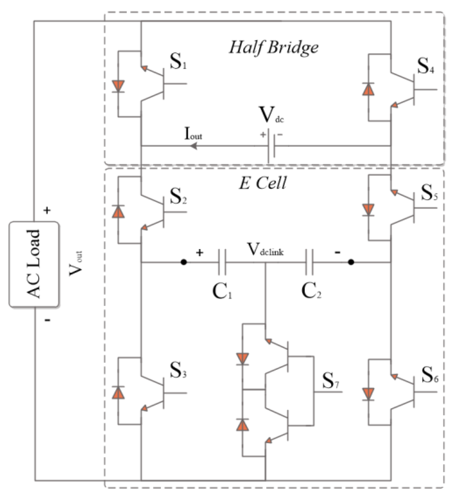
Figure 2.
Flow Chart of Proposed Fault Detection Strategy.

Figure 3.
Data Generation Diagram.
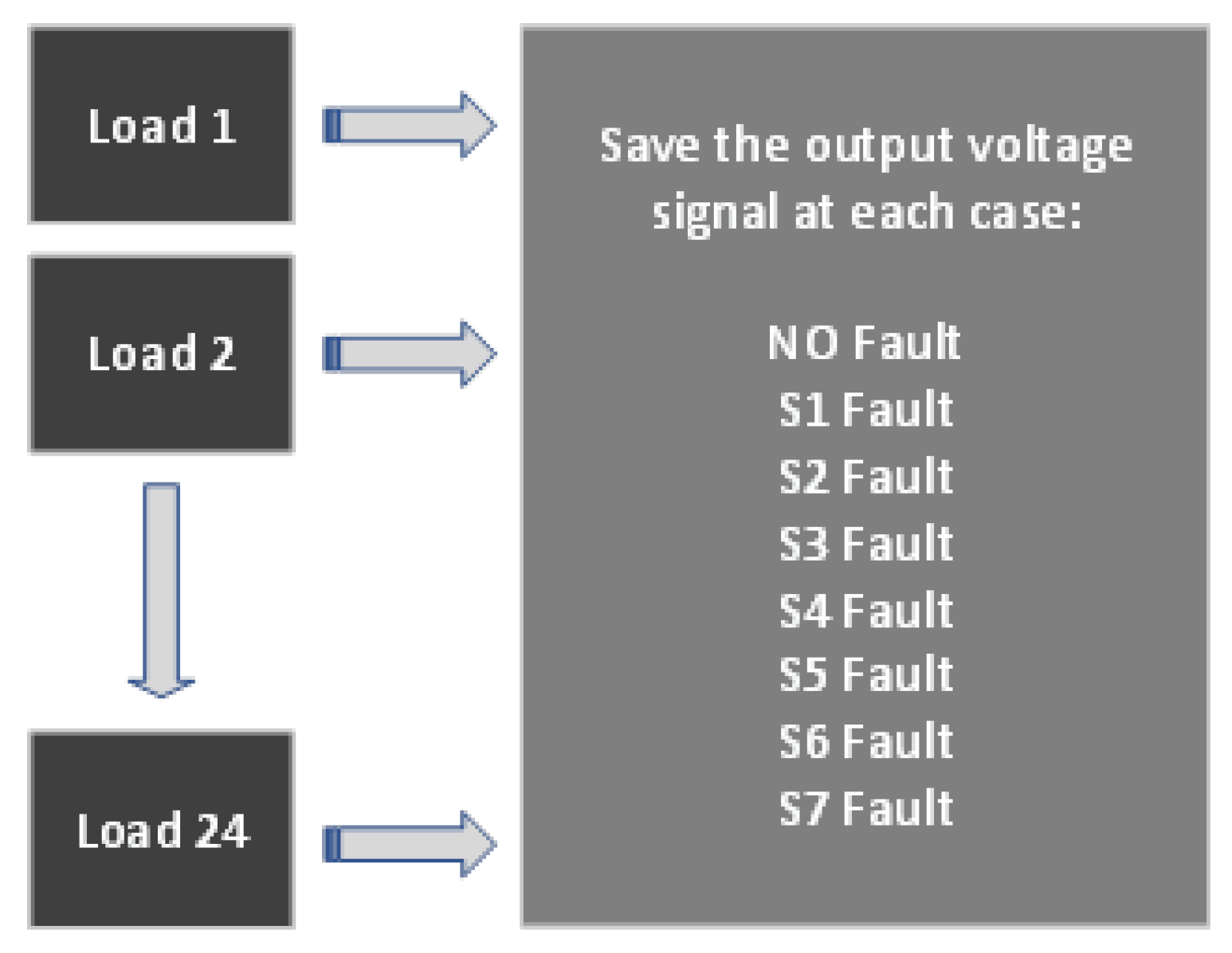
Figure 4.
Histogram Showing Model Accuracy as Function of Different Feature Selection.
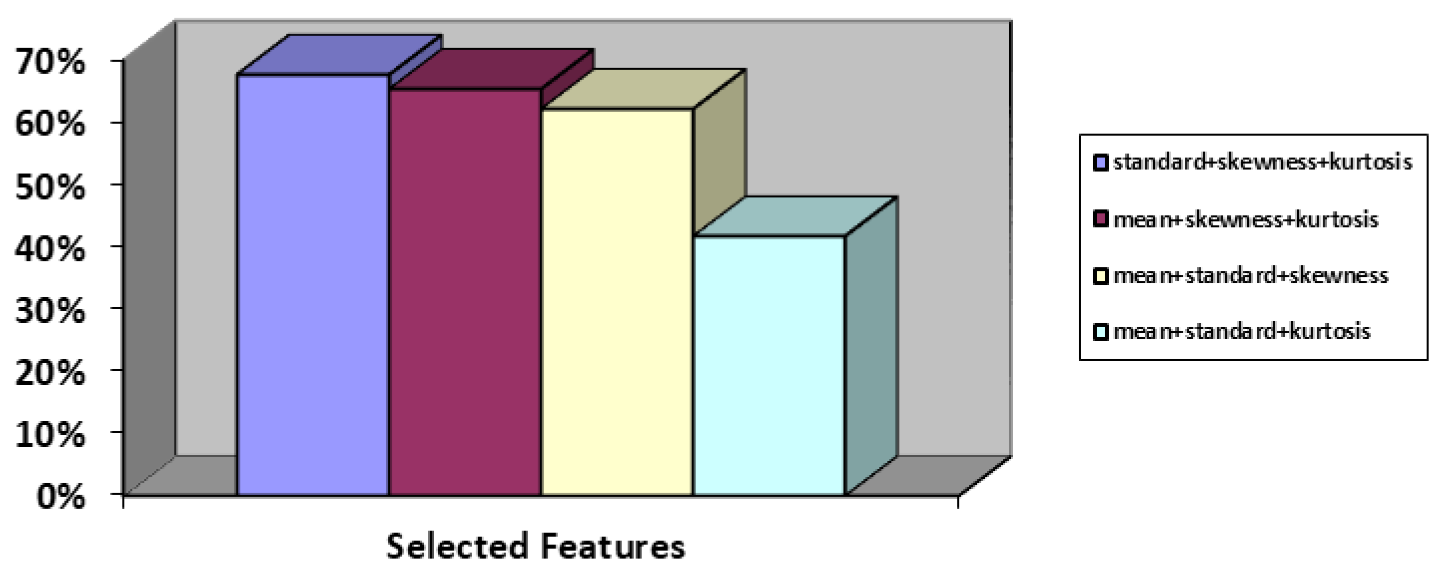
Figure 5.
RFDT Architecture.
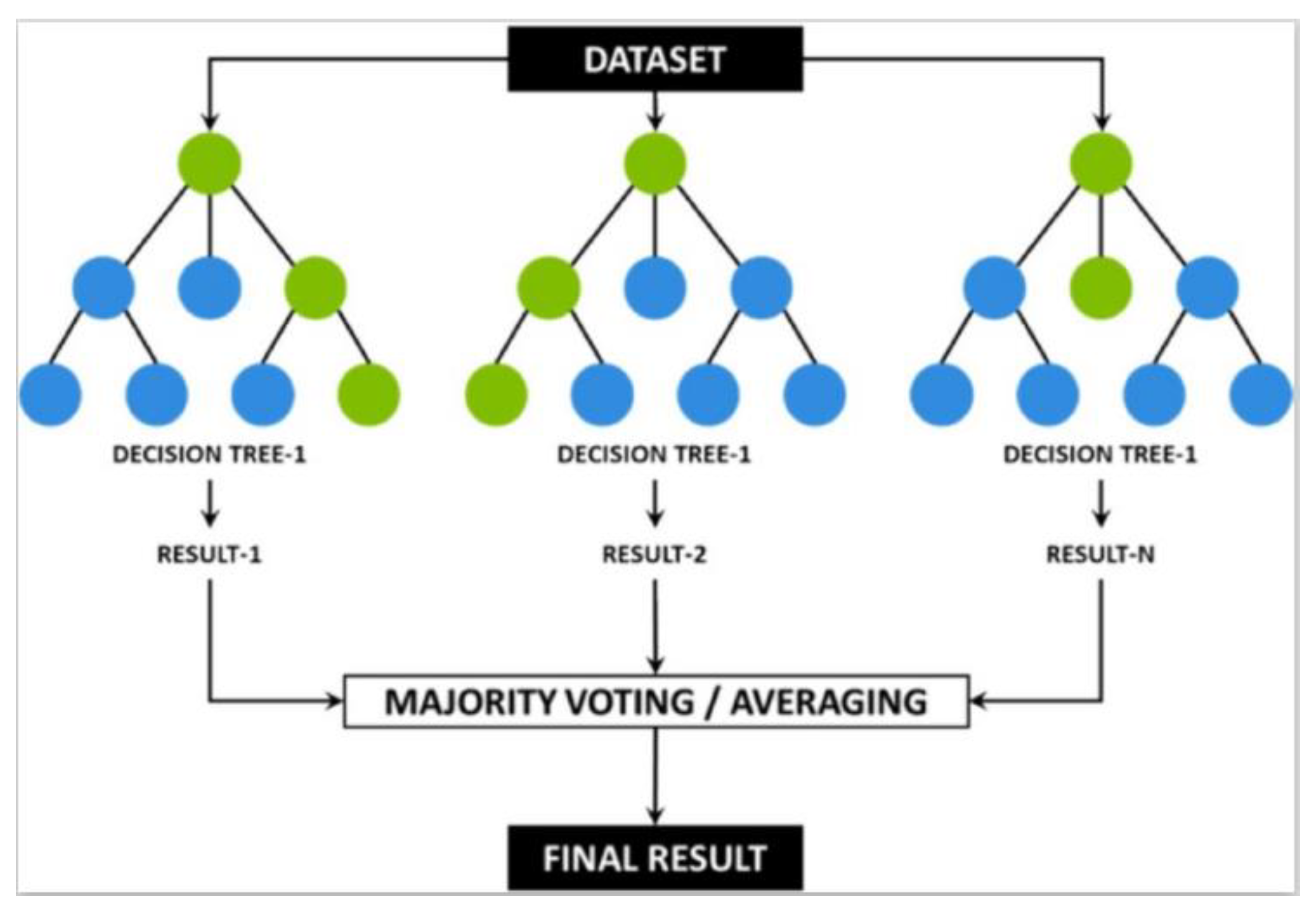
Figure 6.
3D Data Visualization of The Three Selected Features.
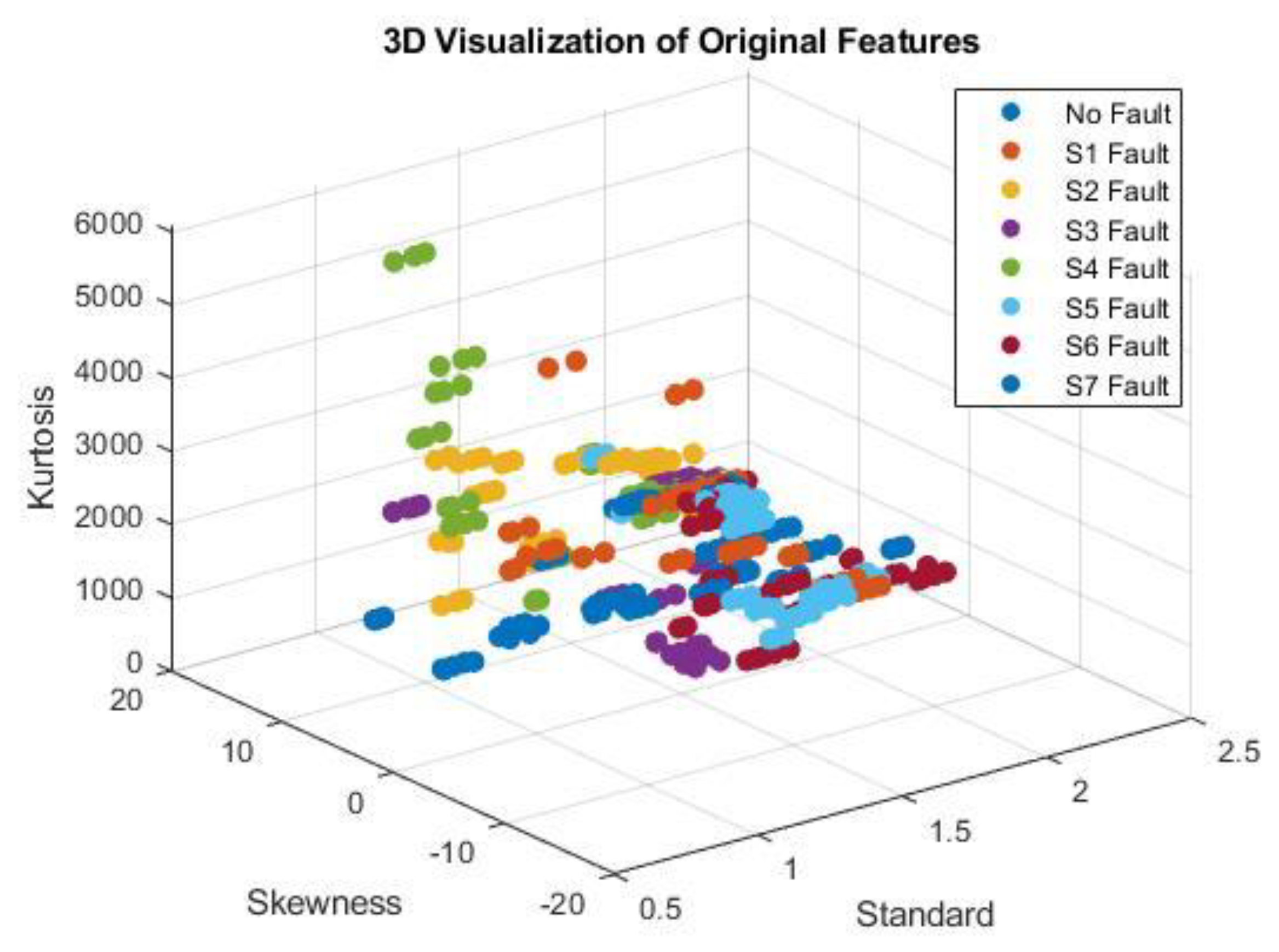
Figure 7.
Architecture of Feed Forward Neural Network Method.
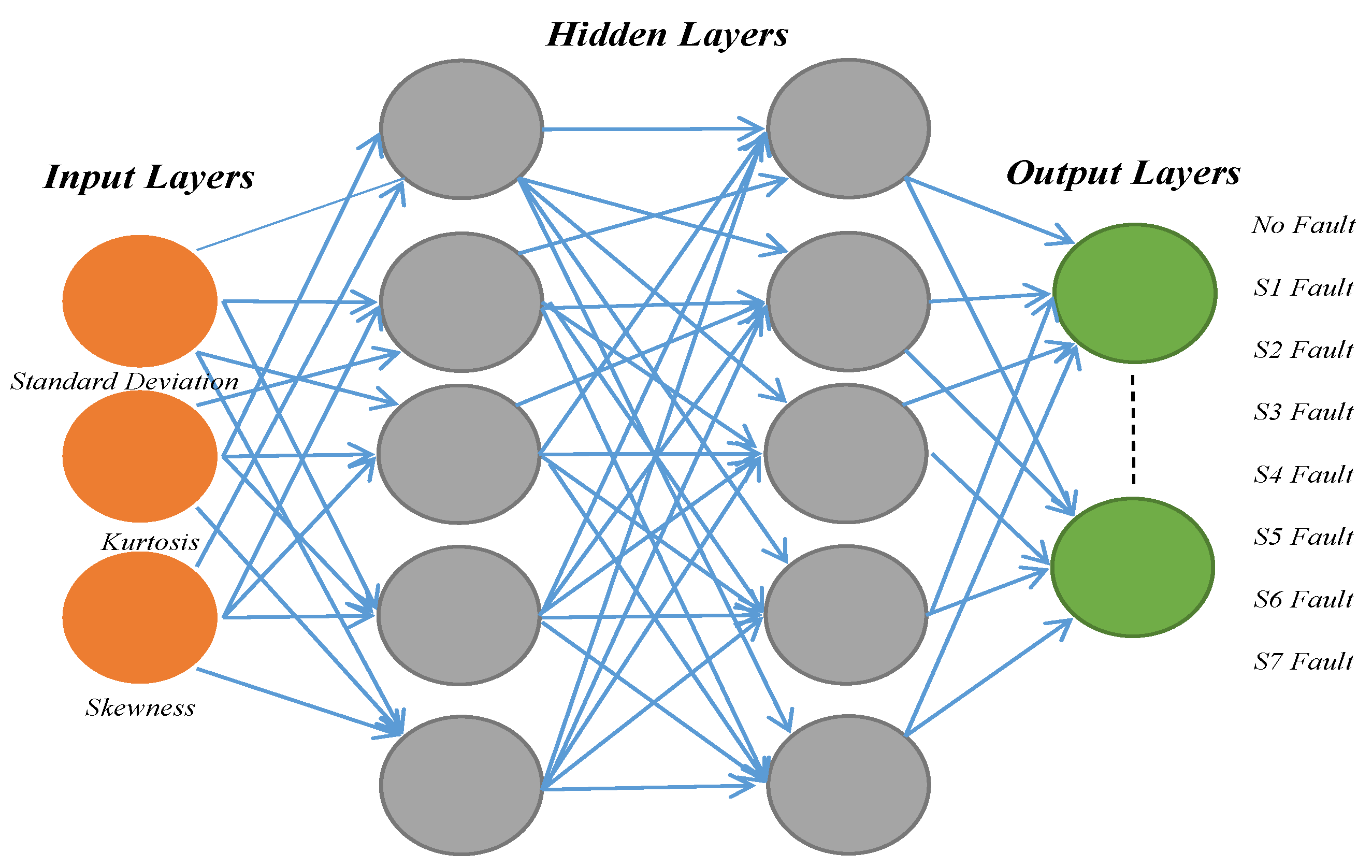
Figure 8.
Flow Chart Showing RFDT Model Training.
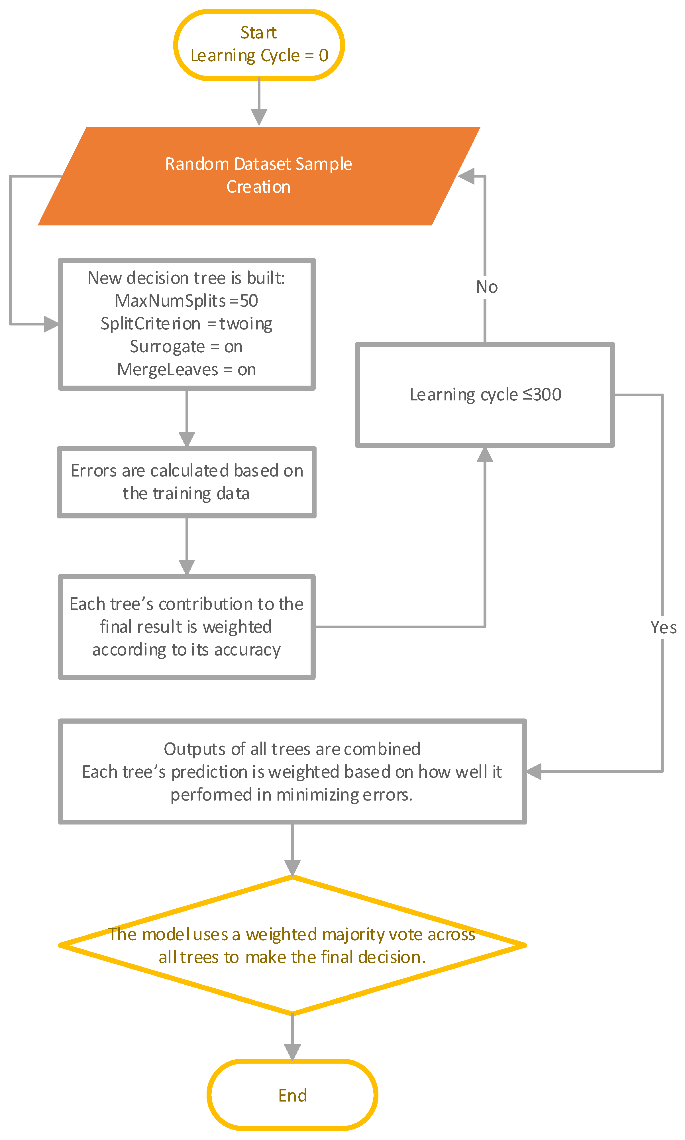
Figure 9.
Flow Chart of Optimization and Training of FFNN Model.
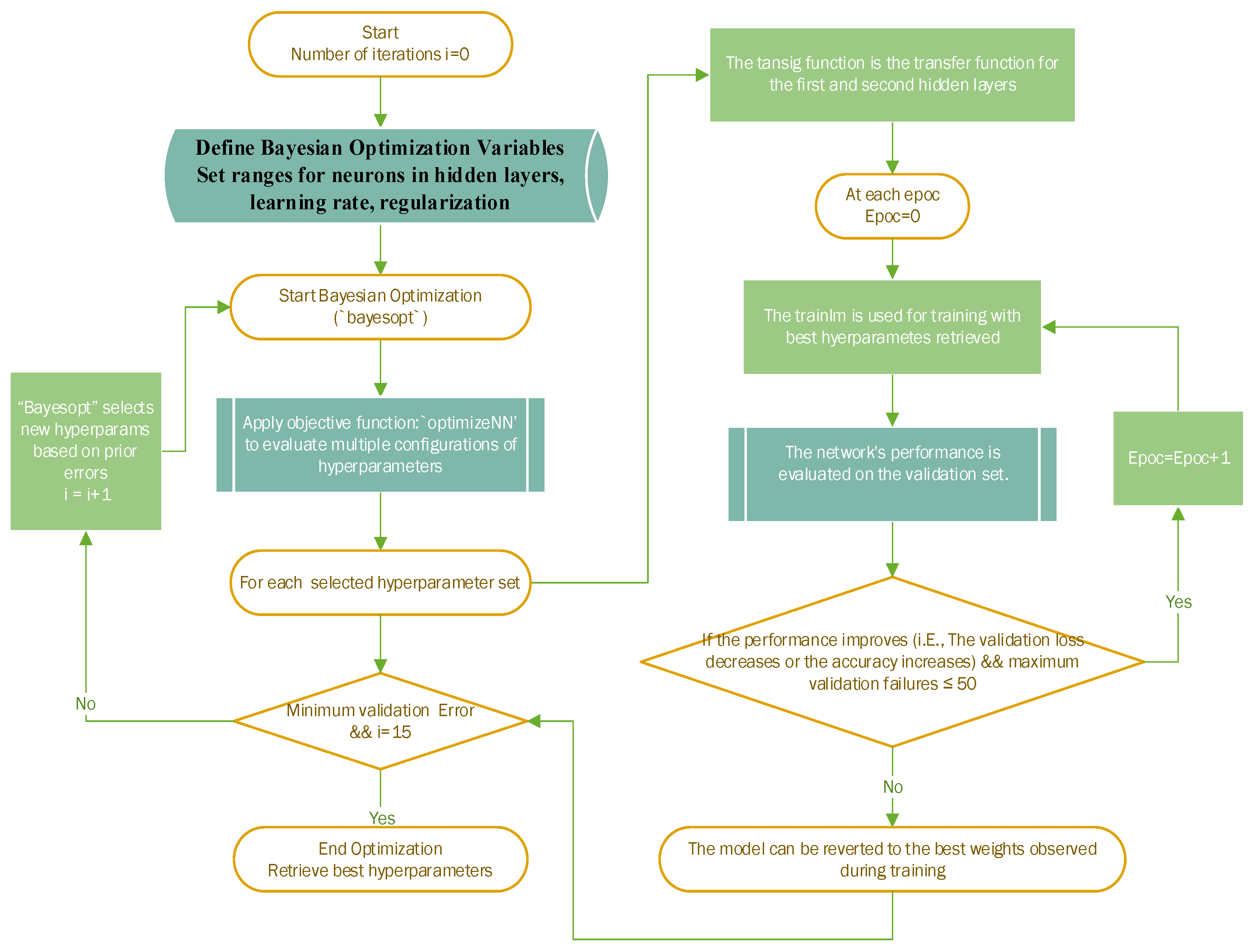
Figure 10.
Error Histogram of the Neural Network during Training and Validation.
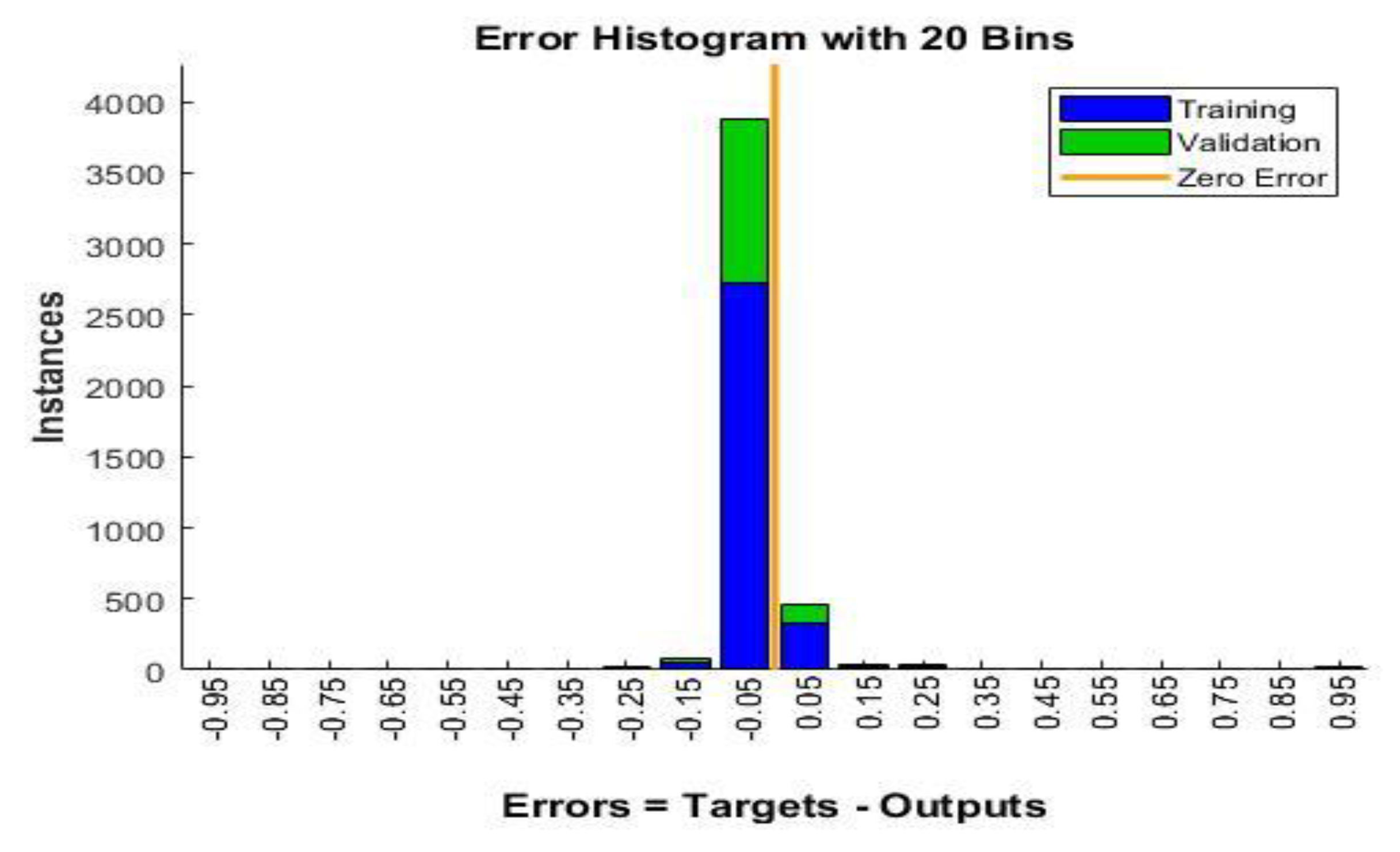
Figure 11.
Performance Graph of Neural Network during Training and Validation.
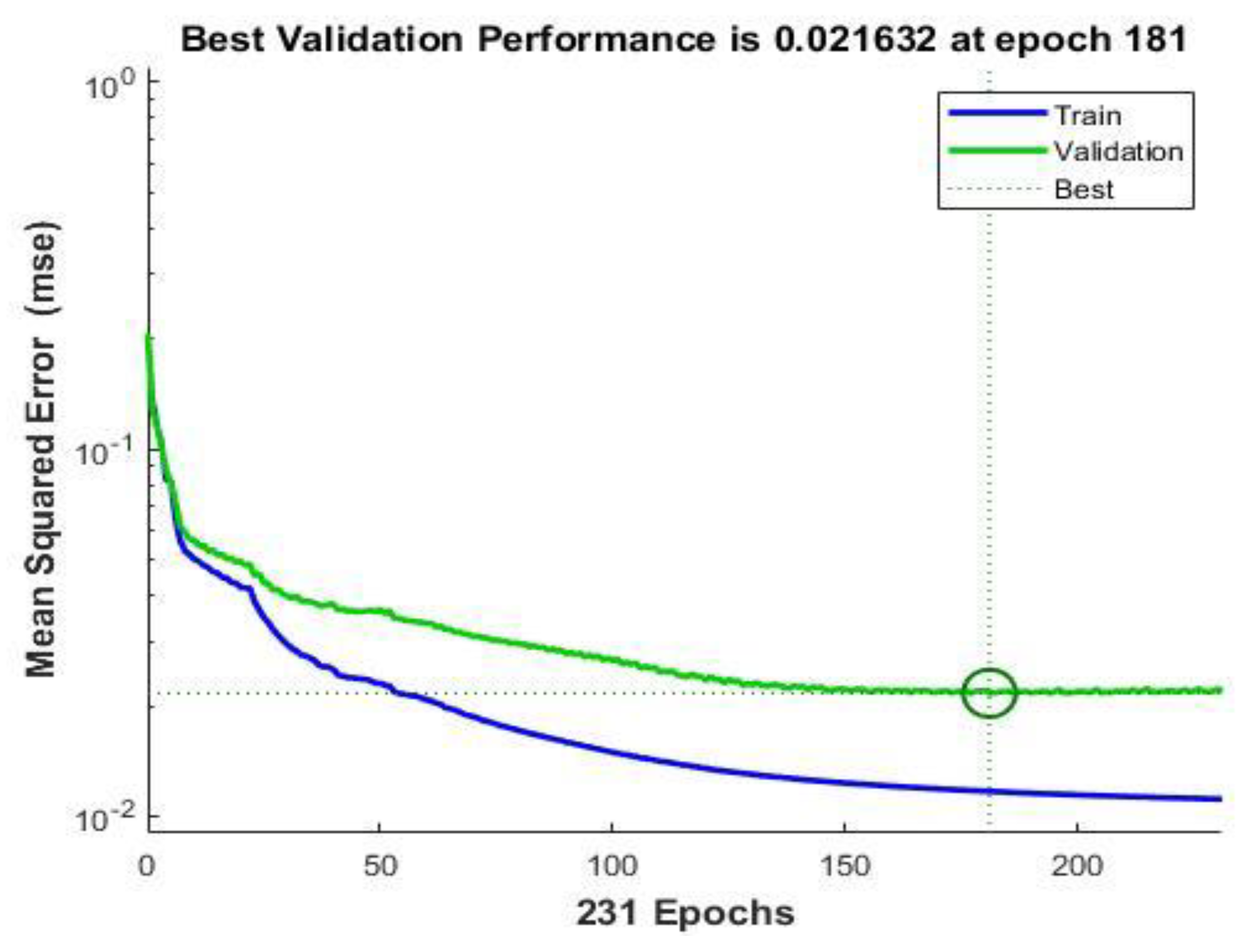
Figure 12.
Confusion Matrix.
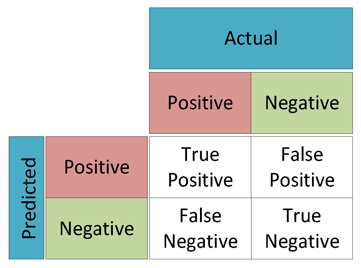
Figure 13.
Graph Showing ROC Curve of (a) Trained Classifier FFNN Model; (b) RFDT Model.
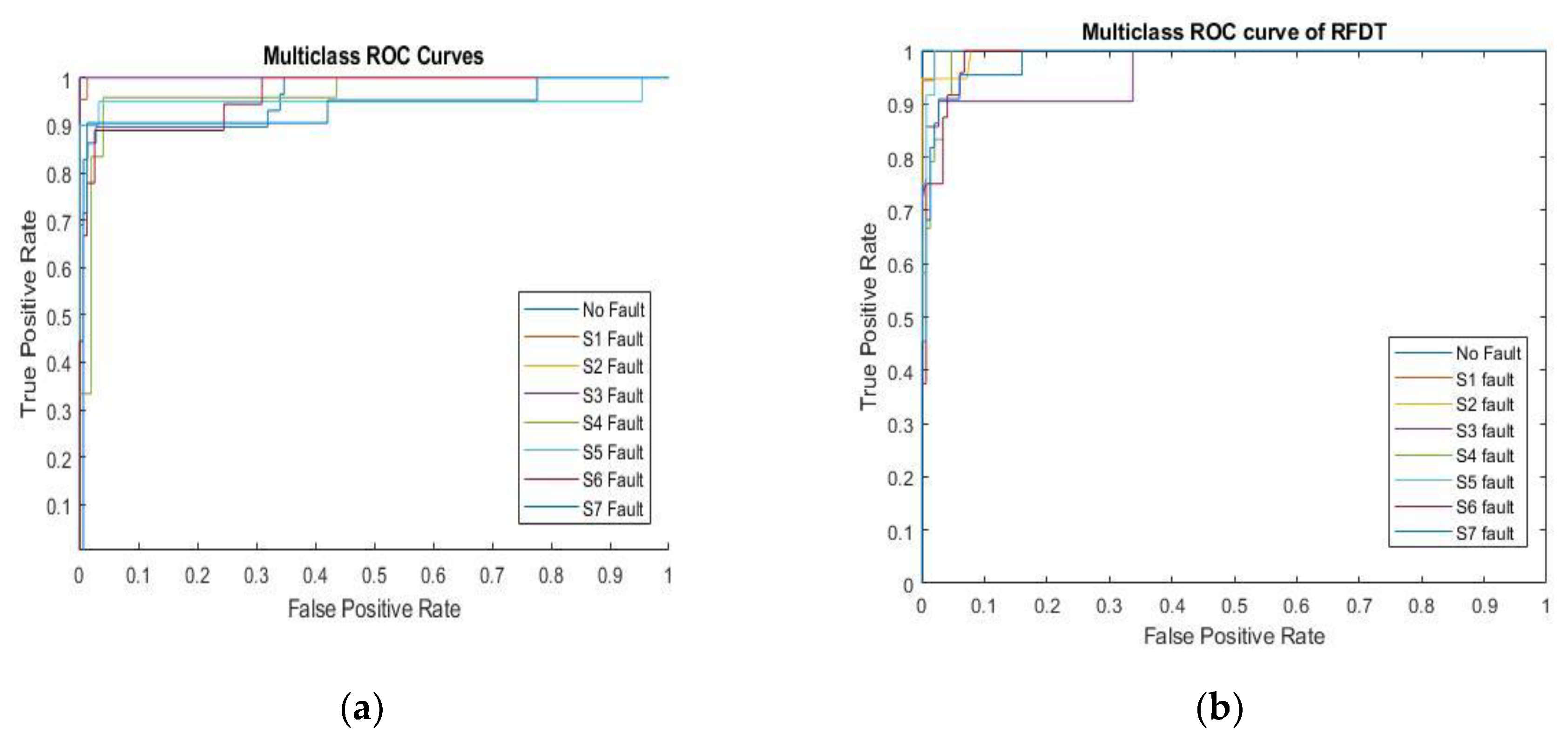
Figure 14.
Graph Showing PR Curve of (a) Trained Classifier FFNN Model; (b) RFDT Model.
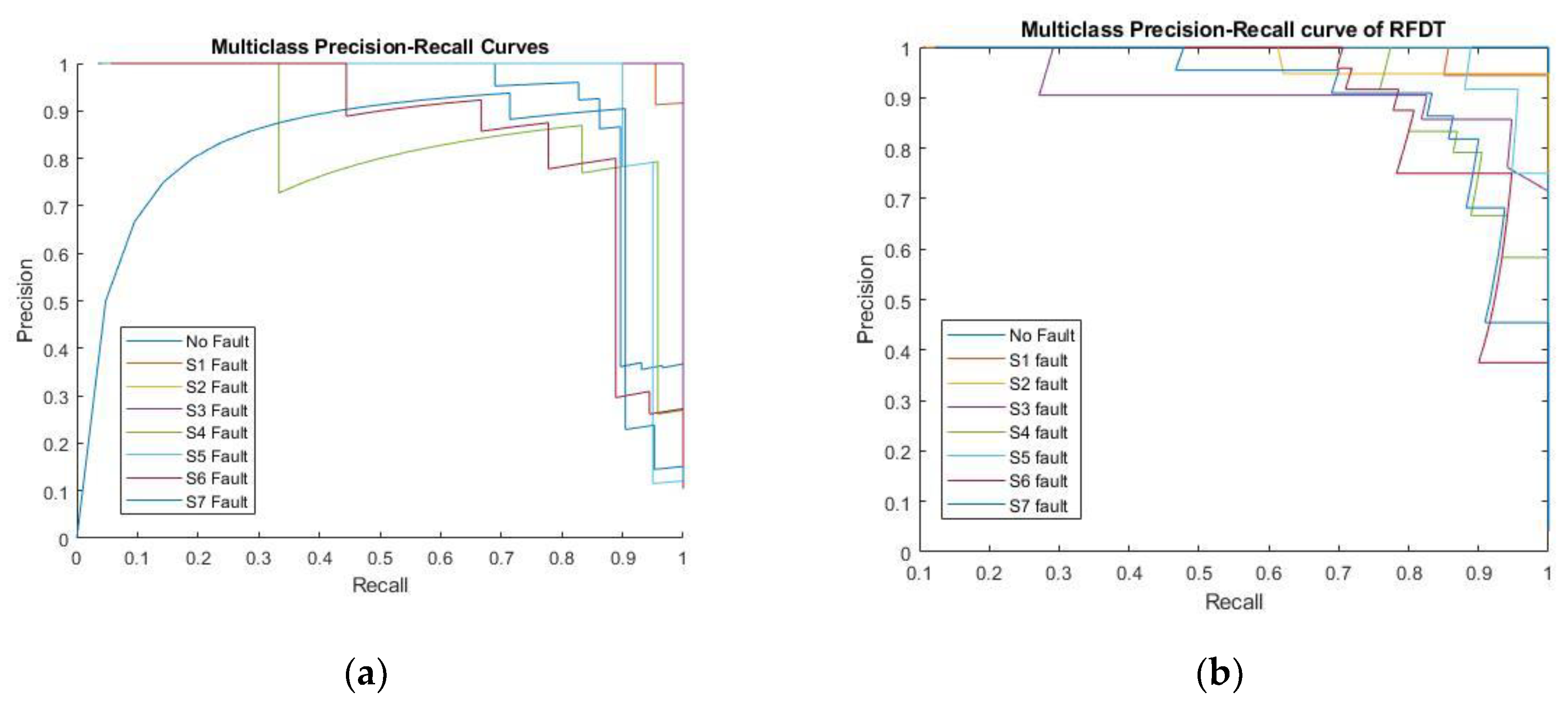

Table 1.
Comparison Table Showing Accuracy for Each Model Classifier.
| Model Classifier | RFDT | FFNN |
|---|---|---|
| Accuracy (%) | 93 | 90 |
| Log Loss Value | 0.56 | 0.72 |
Table 2.
Comparison Table Showing Confusion Matrix for Each Model Classifier.
| Confusion Matrix of RFDT | Confusion Matrix of FFNN |
|---|---|
| 22 0 0 0 0 0 0 1 | 26 0 0 0 1 0 1 1 |
| 0 21 0 0 0 1 1 0 | 0 21 0 0 0 1 0 1 |
| 0 0 24 1 0 0 0 0 | 0 0 20 0 1 0 0 0 |
| 0 0 0 25 0 0 0 0 | 0 0 0 16 0 0 0 0 |
| 0 1 0 0 16 0 0 0 | 3 1 0 0 22 0 0 1 |
| 0 1 3 0 0 21 3 0 | 0 0 0 0 0 17 0 0 |
| 0 0 0 0 0 0 17 0 | 0 0 0 3 0 1 16 1 |
| 0 0 0 0 0 0 0 14 | 0 0 0 0 0 1 1 17 |
Disclaimer/Publisher’s Note: The statements, opinions and data contained in all publications are solely those of the individual author(s) and contributor(s) and not of MDPI and/or the editor(s). MDPI and/or the editor(s) disclaim responsibility for any injury to people or property resulting from any ideas, methods, instructions or products referred to in the content. |
© 2024 by the authors. Licensee MDPI, Basel, Switzerland. This article is an open access article distributed under the terms and conditions of the Creative Commons Attribution (CC BY) license (http://creativecommons.org/licenses/by/4.0/).
Copyright: This open access article is published under a Creative Commons CC BY 4.0 license, which permit the free download, distribution, and reuse, provided that the author and preprint are cited in any reuse.


