
Submitted:
25 February 2025
Posted:
27 February 2025
You are already at the latest version
Abstract
This report introduces a differential capacitance accelerometer principle and the implementation of a reference design, modification of design to meet the design specifications defined for the Range of Motion (ROM) analysis application. The modified design is analysed for its structural and operational stability and evaluated against the design specification and standard design criteria. With the proposed model the sensitivity of 4.62 fF/g was achieved and around 15 mV/g of sense voltage.
Keywords:
MEMS Design
; FEM
; CAD modeling
; Viscous Damping
; Range of Motion
1. Introduction of Device and Need
Accelerometer, as a MEMS device is a critical sensor in consumer products like smartphones, activity trackers and automotive applications. We are targeting this this device for activity monitoring specifically range of motion for rehabilitation purposes. Here is why there’s a need for this device:
Progressively increasing the range of motion (ROM) during rehabilitation is crucial to prevent muscle and joint stiffness maintains or restores flexibility, and helps prevent the formation of scar tissue. Monitoring range of motion (ROM) during rehabilitation can be challenging due to human error, inconsistency, and limited real-time data. Smart sensors could offer access to accurate and objective ROM measurements. They could track progress consistently, identify deviations, and alert therapists to potential issues and open the chance for remote monitoring, progress tracking and providing real-time, data-driven insights to guide and personalize the rehabilitation process.
Using an accelerometer to detect and measure the motion of the human body is one of its applications. Here, we design a surface-machined accelerometer for the measurement of the range of motion application for our rehabilitation device. The measurement range is from -4g to +4g which should have a minimum bandwidth of 4 kHz for the general operation range. The accelerometer is of differential capacitance type and it is chosen based on the benefits in sensitivity, temperature stability and design flexibility it offers.
2. Methodology
For this study, we followed a standard methodology workflow as presented in Figure 1 starting from our reference design. Moreover, the additional branches in analytical and simulation studies are further mentioned in section 3 onwards based on assumptions and conditions we have considered for this model.
3. Problem Definition for Accelerometer
3.1. Assumptions for Modeling
We have considered the following assumptions for the accelerometer modelling:
- Accelerometer is symmetric around central axis.
- Both structures (up/down) are moving as a unified body.
- Accelerometer doesn’t suffer from brittleness or cracks as per selected material.
- Accelerometer is subjected to motion in the lateral axis.
- The cross-sensitivity of the accelerometer in the Y-axis and Z-axis is below 1%.
3.2. Boundary Conditions
The following Table 1 presents the boundary conditions for our accelerometer.
3.3. Meshing Conditions
We have optimized the balance between computation power and meshing quality. After trial and error, the following meshing conditions appeared to be suitable for COMSOL modelling as shown in Table 2. The curvature factor for our electrode fingers was important as well as for spring dimensions. It was observed that physics-controlled meshing also does the job but our approach to go from "Fine" to "Coarse" where possible was using Triangular meshing resulted in about 1.5 hours reduced from a total of 6 hours.
4. Accelerometer Reference Design
We have considered a reference study from [1]. In the referenced model, a surface micromachined design of differential capacitance accelerometer for seismic applications ranging from -50g to +50g is proposed. The accelerometer model from the paper is redesigned as shown in Figure 2. The reference design is for a wide acceleration range and the sensitivity it provides in terms of Δx / g is 1.188 nm/g which is very small and there will be challenges in developing a readout circuit.
We have modified the model and tailored it for ROM application from [1]. In the modification, this sensitivity is addressed. In the reference model, the folded beam spring structure used [2] in has a folded beam at the centre with two free beams on either side without any loading. We have replaced it with folded beams connected in series which effectively improved the sensitivity of the accelerometer to 15nm /g for our application.
5. Study of Accelerometer Design
The accelerometer is designed by keeping the reference design in mind. The differential capacitance is a good solution to enhance the sensitivity.
5.1. Working Principle of Differential Capacitance Accelerometer
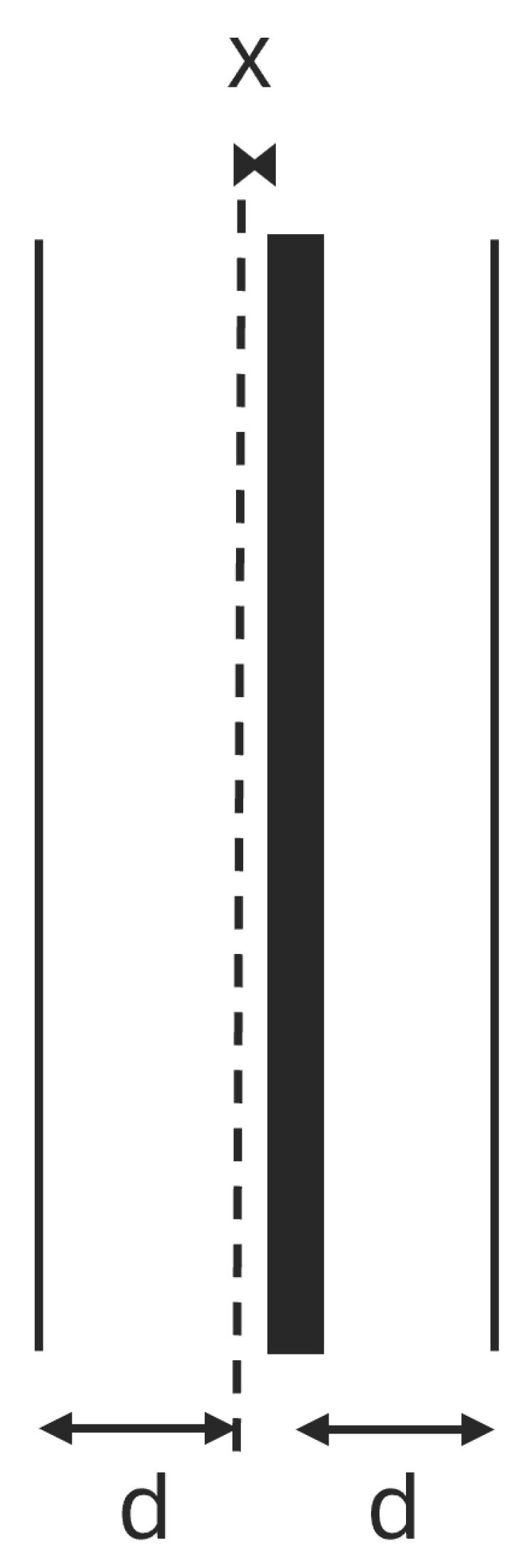
The accelerometer design consists of a proof mass which is suspended by the folded beam spring on either side and the fingers attached to the proof mass can move between the electrodes according to the displacement of mass. The finger in between two electrodes is equivalent to two capacitors attached in series with the finger as the common plate. The displacement of the finger creates a capacitance difference between two capacitors and this is proportional to the acceleration.
where d is the distance between the electrodes, x is the variable displacement, A is the overlap area, and ε is the permittivity of free space. C1 and C2 are the capacitance from the left and right sides of the electrodes. The C in Equation (4) is non-linear, but considering x ≪ d, the Equation (4) can be written as in Equation (5).
The inertial force acts on the system is,
where, k is the spring constant, m is the mass of the design, and a is the acceleration, with F as Force applied to the system. From Hooke’s law, the relationship between Force act and deflection in spring given by the Equation (7), which is the displacement of the proof mass. From Equations (5) and (8), the Equation (9) can be deduced and the differential capacitance directly proportional to acceleration is shown.
 where b is the damping coefficient with other parameters as previously defined. The general spring mass damper model can be considered and the differential Equation (10) can be derived and the second order transfer function can be written as Equation (11) [1]. The parameters which can be used to evaluate the accelerometer design are extracted from the governing function and provided in Equation (12) to (13). The Quality factor (Q) determines the stability of the system based on the type of damping achieved and the resonance frequency (ωr) provides the bandwidth.
Figure 3.
Illustration of electrodes and finger as differential capacitors
5.2. Analytical Calculations
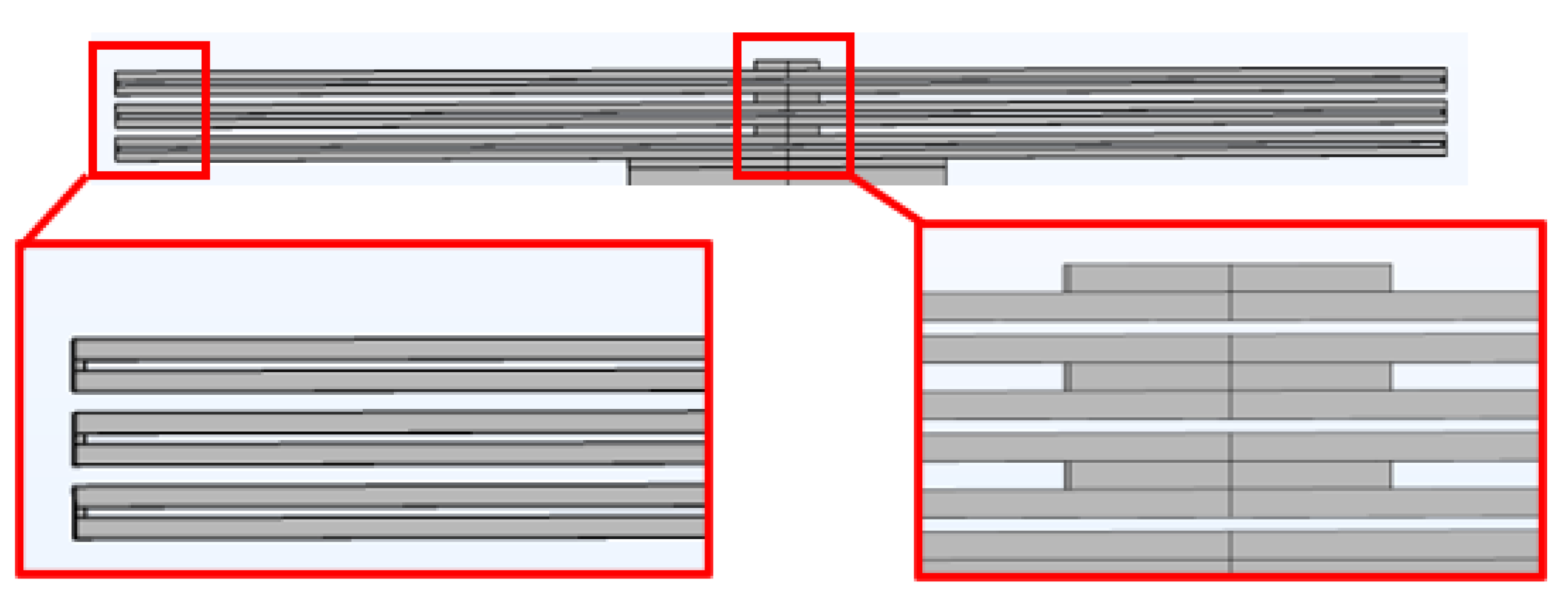
The spring constant of the guided beam structure determines the displacement magnitude of the proof mass and factor to design the accelerometer’s sensitivity as required. The reference model’s [1] sensitivity is not adequate for our application and thus the spring beam design to folded beams connected in series. The spring structure of the accelerometer is a closed guided beam structure as given in Figure 4a. The spring constant of the beam structure is given by Equation (14); where E is the Young’s modulus, L1,L2 is the length of a guided beam, H is the thickness along the axis of deflection and W is the width of the beam. The one-half of the beam spring structure is given in Figure 5 and it shows how three folded beams join together to form the complete beam structure. The two folded beams are similar and the third one connected to the proof mass has different L since part of it is connected together with the proof mass. These three folded beams are in series as the force applied is the same and this spring set is in a parallel configuration to the folded beam structure on the other side of the proof of mass.

Table 3.
Parameter Values and Remarks
| No | Parameters | Value | Remark |
|---|---|---|---|
| 1 | Proof of mass Length | 448μm | suspended mass |
| 2 | Proof of mass Width | 200μm | suspended mass |
| 3 | No of Sensing fingers | 42 | - |
| 4 | No of Driving fingers | 12 | - |
| 5 | Length of fingers | 140μm | electrode connected with mass |
| 6 | Width of fingers | 4μm | electrode connected with mass |
| 7 | Number of perforations | 150 | perforation 110μm on proof mass |
| 8 | Width of hole (square) | 4μm | perforation hole dimension |
| 9 | Thickness of Proof mass | 2μm | surface polysilicon thickness |
| 10 | Beam Length (folded) | 420μm | Ref-design - 380μm |
| 11 | Beam Width (folded) | 2μm | Ref-design - 2μm |
| 12 | Capacitance gap | 1μm | The gap for displacement |
| 13 | Spring beam Length | 420μm | Total length of beam |
| 14 | Spring beam Width | 2μm | Width of beam |
Table 4 shows the dimensions used for the calculation of the spring constant. The effective spring constant of one side compound folded beam is given by the Equation (15) where the k1 denotes the spring constant of middle and folded beam connected with anchor and k2 denotes the spring constant of folded beam fixed with proof of mass. The total spring constant of beam structure is given by kT in Equation (16) and the analytical value of k by substituting the values is 0.2546476 N/m.
The change in capacitance against acceleration is the measure of sensitivity and the proportional voltage change which is used to sense and quantify the acceleration. Equation (4), is used to calculate the ΔC per g unit of acceleration. The ΔC/g is calculated as 4.62 × 10⁻¹⁵ F/g.
The damping coefficient (b) is from simulation and determined as (1.54 × 10⁻⁵) and the Proof of mass is calculated with the assumption of cuboidal block with extended beams (fingers) and through holes with sqare openings and have constant density. The analytically calculated ωr and Q together with sensitivity analysis results tabulated in Table 5.
We have modifications from reference design Figure 3 for spring design. These changes are presented in Figure 6.
Figure 6.
Redesigned Folded Spring Structure
6. Sensitivity Analysis
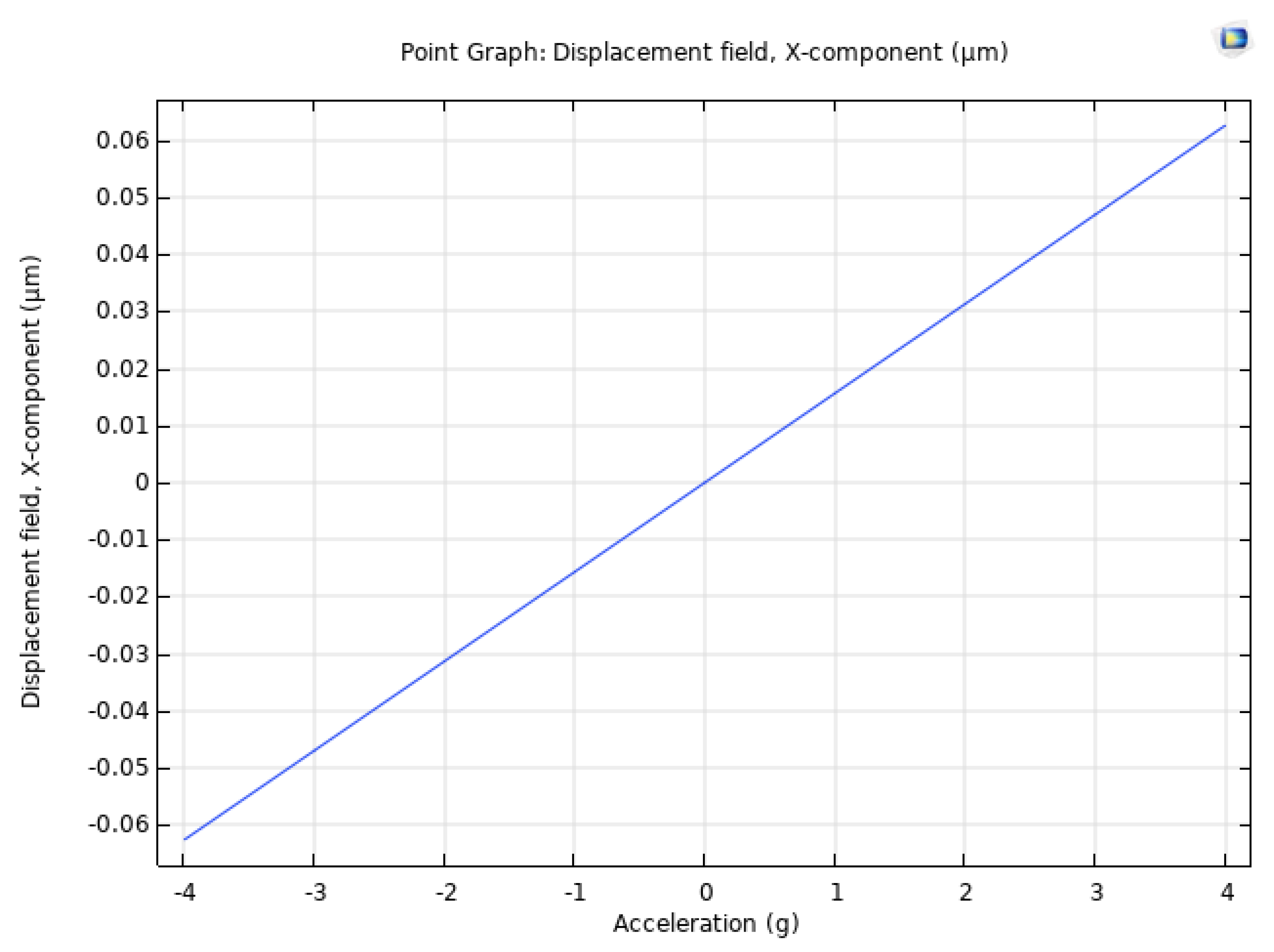
A parametric study is done to analyse the displacement of the mass due to acceleration in the range from -4g to +4g. It follows that at an acceleration of 1g, we obtain a maximum mass displacement of 15nm implying that the sensitivity along the x-direction is 15nm/g.
Figure 7.
Sensitivity in X-axis
Hence, with the parametric study of acceleration, a linear graph is obtained between displacement and acceleration along the x-direction.
Figure 8.
Displacement vs Acceleration
For this accelerometer, the acceleration range was obtained in non-linear mode as shown in Figure 9 and it has been observed that this can be tuned up to +-16g as can be seen in the model of IMU that was used at Aalto university where as per application it was selected from +-4g to +-16g/ [4].
Figure 9.
Non-linear Behavior of Accelerometer
6.1. Cross Sensitivity Analysis
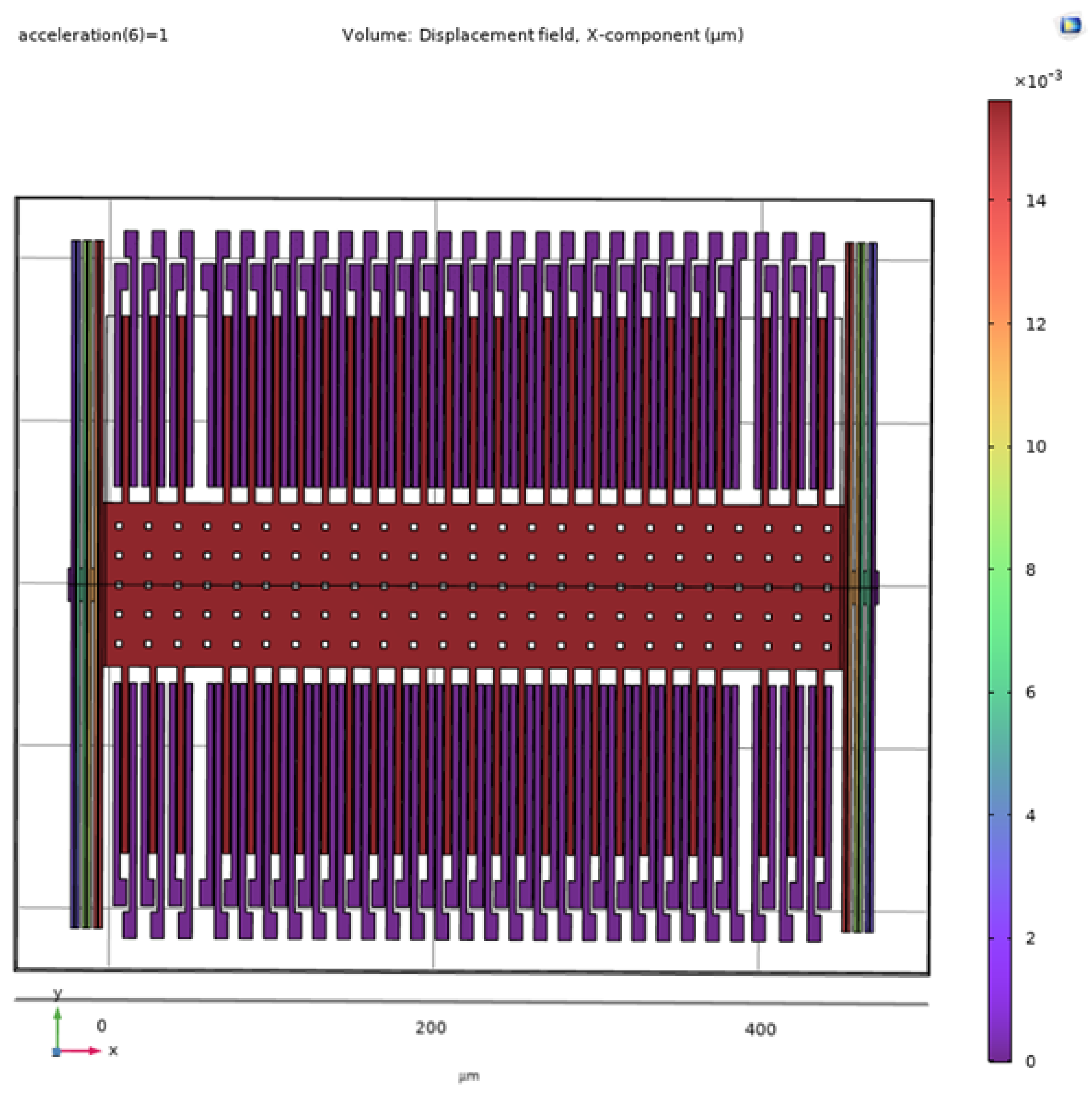
The cross-axis sensitivity of accelerometers refers to the extent to which acceleration measured in one axis affects the readings in other orthogonal axes. Various accelerometer designs aim to minimize cross-axis sensitivity to enhance accuracy. The 3-D accelerometers in literature recommended low cross-axis sensitivity of less than 1%, ensuring accurate measurements in each axis [5]. Additionally, the dual-axis fibre optic accelerometer in [6] demonstrates a cross-axis sensitivity below 5.1%, maintaining measurement accuracy in two perpendicular directions. Furthermore, a modified mechanical-optical model addresses cross-axis interference, achieving a significant increase in accuracy when subjected to cross-axis acceleration [7]. These advancements highlight the importance of minimizing cross-axis sensitivity for precise accelerometer measurements in various applications. As per the suggested literature, we aimed to optimize the cross-sensitivity below 1% and results for cross-sensitivity per g are presented in Figure 10 and Figure 11 as compared to actual x-axis sensitivity illustrated in Figure 7. The simulation from COMSOL shows the sensitivity of 15mV/g as shown in Figure 12.
7. Eigen Frequency Analysis
The operation frequency of the accelerometer needs to be well below the resonance frequency. To meet the criteria, we have performed Eigen Frequency analysis to check the resonating modes in COMSOL. The model provides eigenfrequency values at various vibration modes, except the first eigenfrequency all other modes of vibration show out-of-plane or torsional vibration as per the simulation results. The lowest Eigenfrequency, which is in the same plane as the intended direction of operation is 4kHz as shown in Figure 13. The resonance frequency at around 4 kHz provides enough bandwidth; considering our range of motion application for patient monitoring. The out-of-plane vibration of the model at 7kHz resonance is provided in Figure 14.
8. Stress Analysis
The structural integrity of the accelerometer during it’s operational range and during edge cases of the application scenarios is critical. The beam springs and joints receives the maximum stress during the operational acceleration range in the order of 1 MPa and the maximum bearable stress by polycrstalline silicon is demonstrated in [8] as 930 MPa. The Figure 15 shows the stress distribution and Figure 16 shows the zoomed image of it at the +4g acceleration. The maximum stress from the simulation results is 1.03 MPa, which is well below the maximum allowable stress.
9. Damping Analysis
9.1. Squeeze Film Damping
The interaction between movable microelectromechanical (MEM) components and the air enveloping them leads to alterations in their dynamic behaviours. These alterations impact various parameters such as resonance frequency, quality factor, and vibration magnitude. The damping effect in the surface machined accelerometer can be modelled considering the effects of squeeze film, slide film and drag force [9]. The squeeze film damping is prominent when the gas film thickness is less than the one-third of width of the vibrational structure; in our case, the perforated mass width is quite larger than the few um gaps [2]. The squeeze film damping is analyzed with COMSOL simulation, and the slide film is calculated based on dimensions and with equations to estimate its effect.
As shown in Figure 17, the air film confined between the plate and the adjacent wall experiences compression, inducing an additional pressure within the gap owing to viscous flow dynamics. As the plate separates from the wall, this pressure diminishes. Consequently, the forces acting upon the plate consistently oppose its motion. The mechanical work exerted by the plate during its motion is consequently dissipated as heat. In the equation describing this phenomenon, the force (F) is inversely proportional to the velocity (v) of the plate and is represented by the expression F = -cv, where c denotes the coefficient of damping.
In this work, we aim to address squeeze film damping through experimental investigations. Incorporating the volume of surrounding fluid in the analysis is essential, necessitating computationally intensive 3D models. To alleviate computational burdens, a compact and dimensionally reduced model is proposed in COMSOL, enabling the simulation of complex scenarios.
9.1.1. Analytical Background
For this model, the generalization is considered for incompressible fluid and modified Reynold’s number:
And squeeze number is:
The boundary conditions for the linearized Reynolds equation are: Total pressure (P) is equal to a constant value (), expressed as .The difference between the pressure (P) and the constant value () is zero, expressed as .
9.1.2. COMSOL Model Definition for Squeeze Film
For this project, the simulation encompasses 6 distinct geometric configurations derived from experiments detailed in [2]. Utilizing BAO’s perforation model, the simulation is implemented within the Thin Film Flow physics interface of COMSOL. Additionally, two extreme scenarios are simulated: one without perforations and another with zero relative pressure at the perforations. The frequency domain formulation is applied, assuming a small amplitude first-order harmonic variation of film pressure, film height, and wall velocity at the frequency of concern. In this model, the boundary conditions entail a vanishing relative pressure (pf = 0) at the perimeter of the proof of mass plate. The relative pressure values in the gas film for the frequency domain analysis are depicted in Figure 18, Figure 19 and Figure 20 for the three respective cases. As anticipated, the pressure magnitude is maximal for the extreme scenario with no etch holes, and minimal for the scenario with zero relative pressure within the etch holes.
In the current model, if the perforations decrease or increase, the pressure on the plates keeps increasing. However, the optimal value where the balance between the mass of the plate and perforation scenario is achieved at a number of perforations along length of 25 and along width at 6 as shown in Figure 21.
The damping coefficients for three cases are obtained and shown in Figure 22.
Upon further investigation, we noted that although other parameters like number of perforations, length, width and central frequency do affect the squeeze film damping coefficient not as much as the gap height. Therefore, keeping all the values listed in Figure 23. The parametric sweep over a reasonable gap size from 1-6 µm range is selected and an optimal solution is found at solution 4 with a gap height of 2.5 µm as shown in Figure 24.
9.2. Slide Film Damping
The device is enclosed by bonding a glass or silicon wafer and thus the top has a gas gap similar to the bottom and the slide film in sidewalls and in fingers is also taken into account. The slide film force is given by Equation (19) and the damping coefficient depends on the effective area (A), gas gap (d) and kinematic viscosity of air (µ).
The dimensions and constant values stated in Table 6 is applied to the Equation 19 and the slide film damping is calculated as 2.93 × 10⁻⁶ Ns/m. The air drag damping coefficient is given by Equation (20), where l is the characteristic length which is half of the plate width (perforated mass). The air drag-related damping coefficient is calculated as 1.92 × 10⁻⁸ Ns/m
10. Frequency Response and Time Domain Response Analysis
10.1. Frequency Response
For the accelerometer, from the lumped model we have the equations as follows,
From Equation (22), we can observe that as the resonance frequency, decreases, the low-frequency response increases and the high-frequency displacement can be seen as independent of the resonance frequency.
From the calculation, the mass of the design is m = 5.47e-10 Kg. The spring constant value is calculated by solving
where x value arrives from the comsol model for the acceleration of 1g. The spring constant (k) is 3.431e-1 N/m. It can also be seen that the resonant frequency of 3.982 KHz obtained from the k and m values are in congruence with that of the obtained from eigenfrequency simulations.
A rigorous design and analysis is done to find the damping coefficient. The damping coefficient is obtained over a range of values by sweeping the physical dimension parameters over a range as illustrated in Figure 23. By using Matlab code (attached as code 1), iteration is done through a range of b values. It calculates the flatness measure of the magnitude response within the frequency range from 0 to 4000 Hz. The b value that minimizes the flatness measure is considered optimal for achieving a flat response within our frequency range. In this way, we obtain the optimum b value of 1.50e-5 Kg/s as illustrated in Figure 25. Then by simulation in comsol by sweeping the parameters in the proximity range of the desired value of b, the perforation spacing and other related parameters are found. So from the simulation, we obtain the value of b as 1.54e-5 Kg/s for the specific gap height and length parameters as shown in Figure 24.
Putting these values in Equation (22) we draw the magnitude of the transfer function to the frequency to obtain the frequency response as shown in Figure 26.
From this, the ζ, damping ratio obtained is 0.5616, the damping coefficient, b as 1.54e-6 Kg/s with the quality factor, Q as 0.8903, signifying that the system is underdamped. This is not too far from the critically damped condition. The accelerometer should be operated in the low-frequency region, below its mechanical resonant frequency.
10.2. Time Domain Response
Considering our accelerometer design, a circuit, as shown in Figure 27 is created using the basic circuit elements to simulate the time-domain response. The resistance is b (the damping coefficient), the capacitance is 1/k, k is the spring constant, and the inductance is equal to the mass of our design. At the force of 1g acceleration, we receive the response of position versus time as shown in Figure 28. Ideally, the response should be a step function, but a physical accelerometer will always have a delay. The most optimum damping coefficient possible from our design is 1.54e-6 N.m/s which will offer optimal speed with a little overshoot or ringing. As discussed previously, the optimum value of the damping coefficient is reached by simulating various dimensions of the perforations from the simulations. As observed in Figure 28, our system is slightly underdamped, nearer to the critical damping situation with damping coefficient b is 1.54e-6 N.m/s.
11. Noise Analysis
In MEMS devices with the measurement of nanometre range motion Brownian noise is significant and it is from the random motion of gas molecules around the proof of mass and between the electrode and finger gaps. The perforated proof of mass has provided significantly more volume for gas molecule distribution and the effect of it in terms of thermal noise generation could be an interesting analysis. Here, using the Equation (24), where KB is Boltzmann constant, T is absolute temperature, D is viscous damping coefficient and M is the mass of movable part of accelerometer[10].
The material used for the proof-of-mass can also determine the Brownian noise and in [10], it is suggested that Au has the best results in minimizing the noise. Considering mass production and low-cost accelerometers for consumer electronics it is not an applicable option and regardless the b and m can be optimized to minimize the Brownian noise. Since b is mainly determined by squeeze film damping and the optimization of it affects the m as well an optimized design could be reached while considering other factors like Q and ωr. The Brownian noise for our model is calculated using Equation (24) as 21.46 ng/√Hz.
12. Discussion
The differential capacitance accelerometer design presented in this study undergoes a thorough analysis to ensure its suitability for Range of Motion (ROM) monitoring applications in rehabilitation. We achieved a bandwidth of 3KHz and voltage sensitivity of 15mV/g which is sufficient for our target application. Initially derived from a reference model tailored for seismic applications, the accelerometer underwent significant modifications to address sensitivity concerns pertinent to ROM analysis. By replacing the original folded beam spring structure with series-connected folded beams, the accelerometer’s sensitivity was enhanced, aligning it with the precise measurement requirements of ROM monitoring. Theoretical and analytical studies elucidate the accelerometer’s working principle, highlighting its sensitivity, resonance frequency, damping coefficient, and quality factor, essential parameters for performance evaluation. Additionally, capacitance sensitivity in the range of fF/g ensures that suitable read-out circuits can be designed in the upcoming semester, thus realizing the rehabilitation monitoring exercises.
A rigorous investigation of squeeze film damping has provided the optimal gap size of 2.5µm on which the response of the system is underdamped with a Q value of 0.89. Initial analysis through changing the geometry of the perforated plate gave us a deep understanding of optimizing the structure of the Accelerometer from a practical point of view.
The summary of achieved specifications as the COMSOL simulation and the generated graph is given in Table 7.
13. Conclusions
This report presents a design and analysis of a 1-axis capacitive-based comb-drive MEMS accelerometer designed specifically for Range of Motion (ROM) applications. The precise monitoring of muscles is crucial for rehabilitation, as recommended by therapists, necessitating a quick response from the accelerometer. The study demonstrates that viscous damping, influenced by factors such as perforated mass and geometric parameters, plays a significant role in tailoring the system’s response to achieve the desired sensitivity and range. Additionally, the optimization of cross-sensitivity ensures consistent system behaviour across a specified frequency range. By optimizing these parameters, the accelerometer can effectively measure and respond to movements within the required range, facilitating enhanced monitoring of muscle motion for rehabilitation purposes.
14. Declaration of Contribution
All authors have contributed equally this report starting from the literature study until the final draft. The cross-collaboration among teams ensured a comprehensive understanding of the whole review paper and all sections and flows were approved as a team.
References
- Khouqeer, G.A.; Suganthi, S.; Alanazi, N.; Alodhayb, A.; Muthuramamoorthy, M.; Pandiaraj, S. Design of MEMS capacitive comb accelerometer with perforated proof mass for seismic applications. 35, 102560. [CrossRef]
- Bao, M.; Yang, H. Squeeze film air damping in MEMS. Sensors and Actuators A: Physical 2007, 136, 3–27. [Google Scholar] [CrossRef]
- Senturia, S.D. Microsystem design 2001.
- .
- Development of a High-Precision and Low Cross-Axis Sensitivity 3-D Accelerometer for Low-Frequency Vibration Measurement. IEEE Sensors Journal 2023. [CrossRef]
- A High-Sensitivity Dual-Axis Accelerometer with Two FP Cavities Assembled on Single Optical Fiber. Sensors 2022. [CrossRef]
- Accurate mechanical-optical theoretical model of cross-axis sensitivity of an interferometric micro-optomechanical accelerometer. Applied optics 2022. [CrossRef]
- Bromley, S.; Howell, L.L.; Jensen, B.D. Determination of maximum allowable strain for polysilicon micro-devices. Engineering Failure Analysis 1999, 6, 27–41. [Google Scholar] [CrossRef]
- Veijola, T. Chapter 13 - Gas Damping in Vibrating MEMS Structures. In Handbook of Silicon Based MEMS Materials and Technologies (Second Edition); Tilli, M., Motooka, T., Airaksinen, V.M., Franssila, S., Paulasto-Kröckel, M., Lindroos, V., Eds.; William Andrew Publishing; pp. 354–373. [CrossRef]
- Yamane, D.; Konishi, T.; Matsushima, T.; Machida, K.; Toshiyoshi, H.; Masu, K. Design of sub-1g microelectromechanical systems accelerometersa). 104, 074102. [CrossRef]
Figure 1.
WorkFlow for this Accelerometer Design
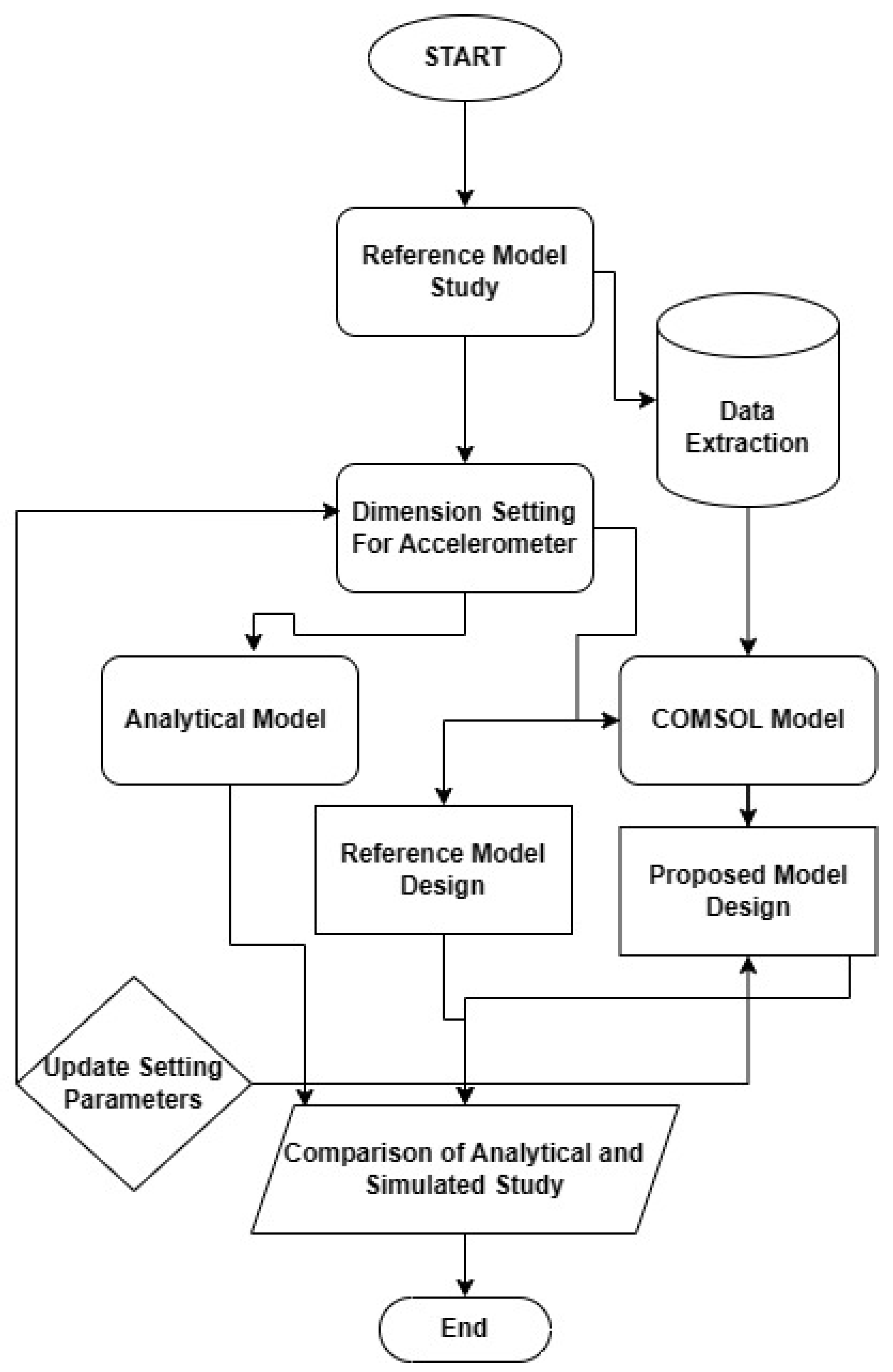
Figure 2.
The differential capacitance accelerometer design illustration from reference paper[1]
Figure 2.
The differential capacitance accelerometer design illustration from reference paper[1]
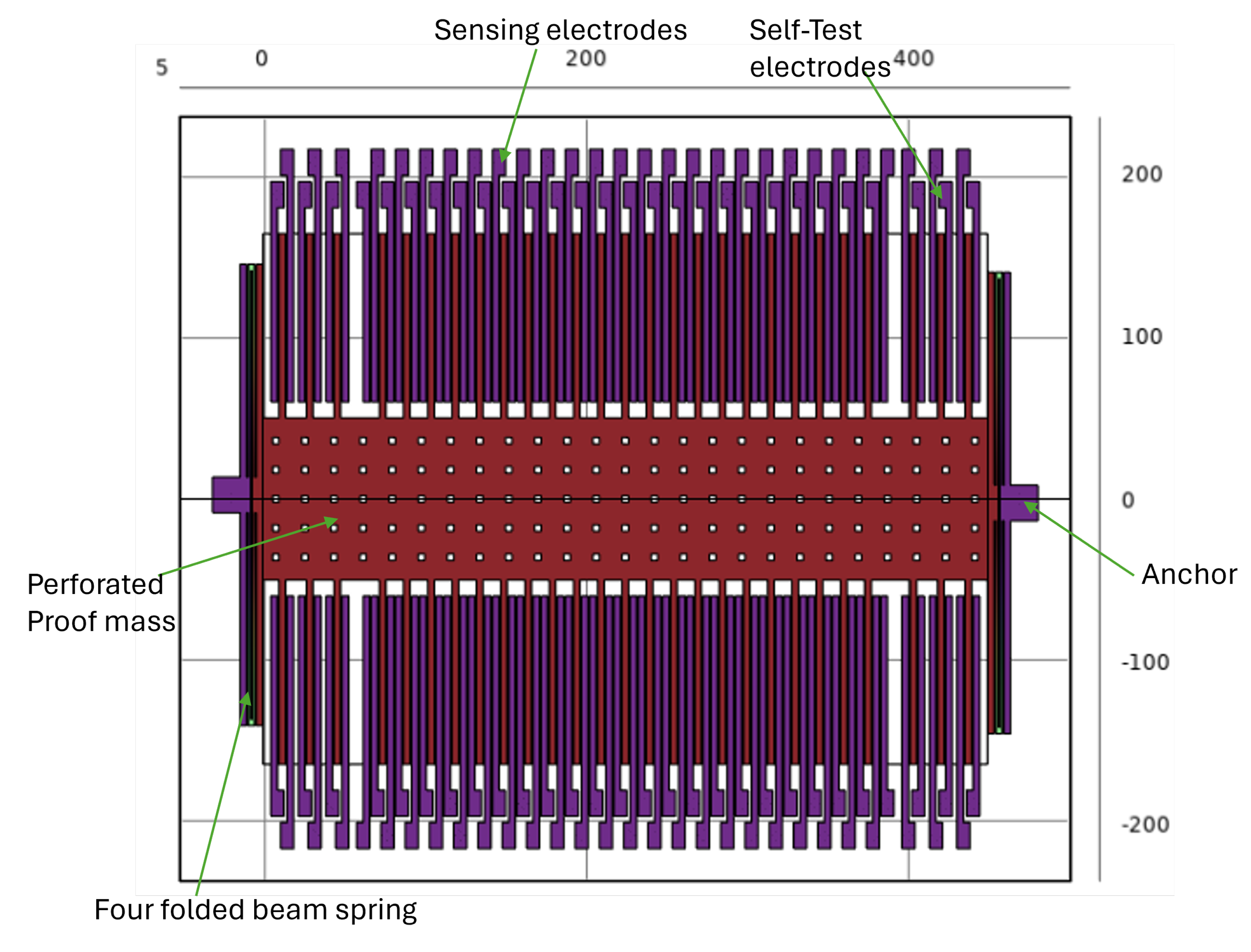
Figure 4.
Folded beam structure and equivalent unfolded beam[3]
Figure 4.
Folded beam structure and equivalent unfolded beam[3]
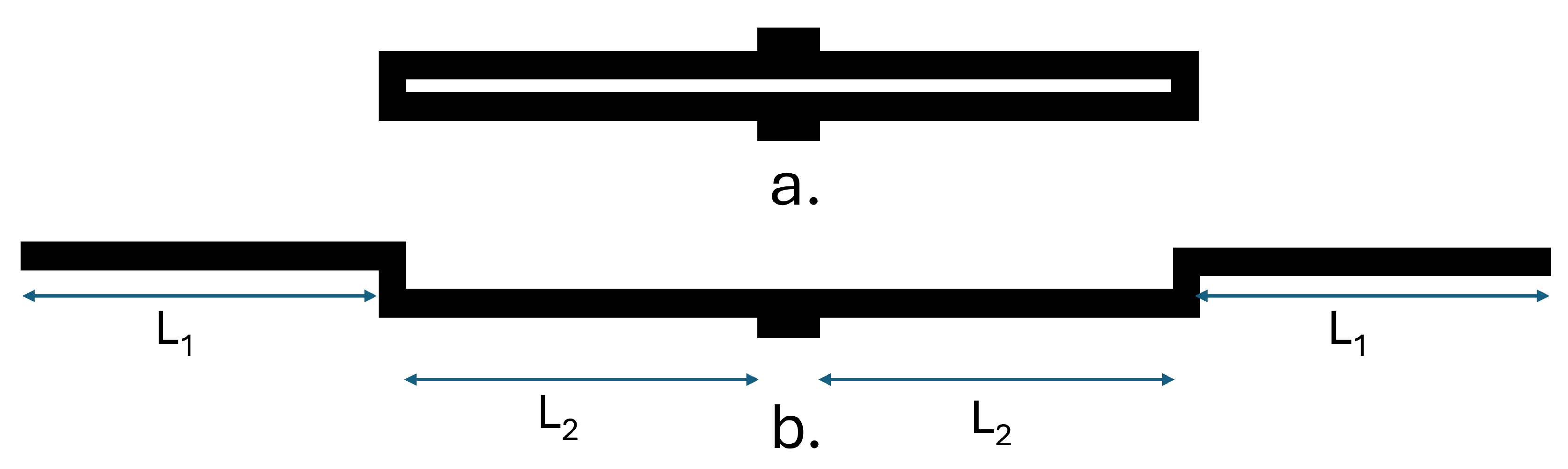
Figure 5.
Schematic of spring structure of the accelerometer, the symmetrical half portion of the compound folded beam structure provided for clear view
Figure 5.
Schematic of spring structure of the accelerometer, the symmetrical half portion of the compound folded beam structure provided for clear view
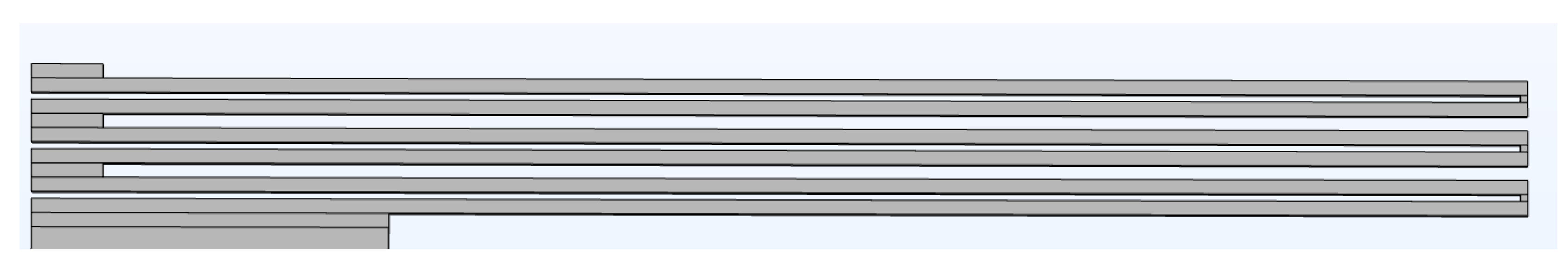
Figure 10.
Cross Sensitivity in Y-axis
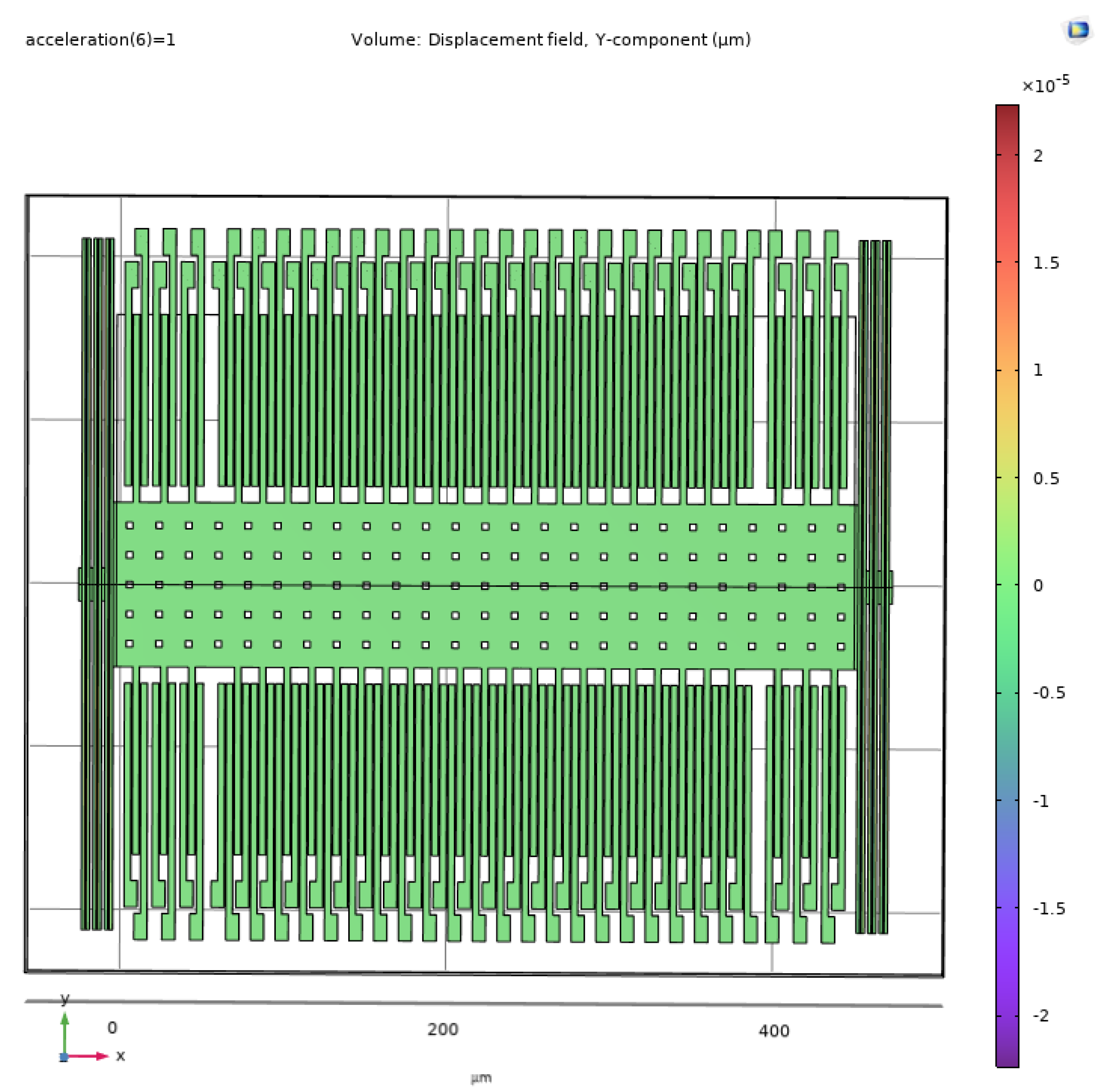
Figure 11.
Cross Sensitivity in Z-axis
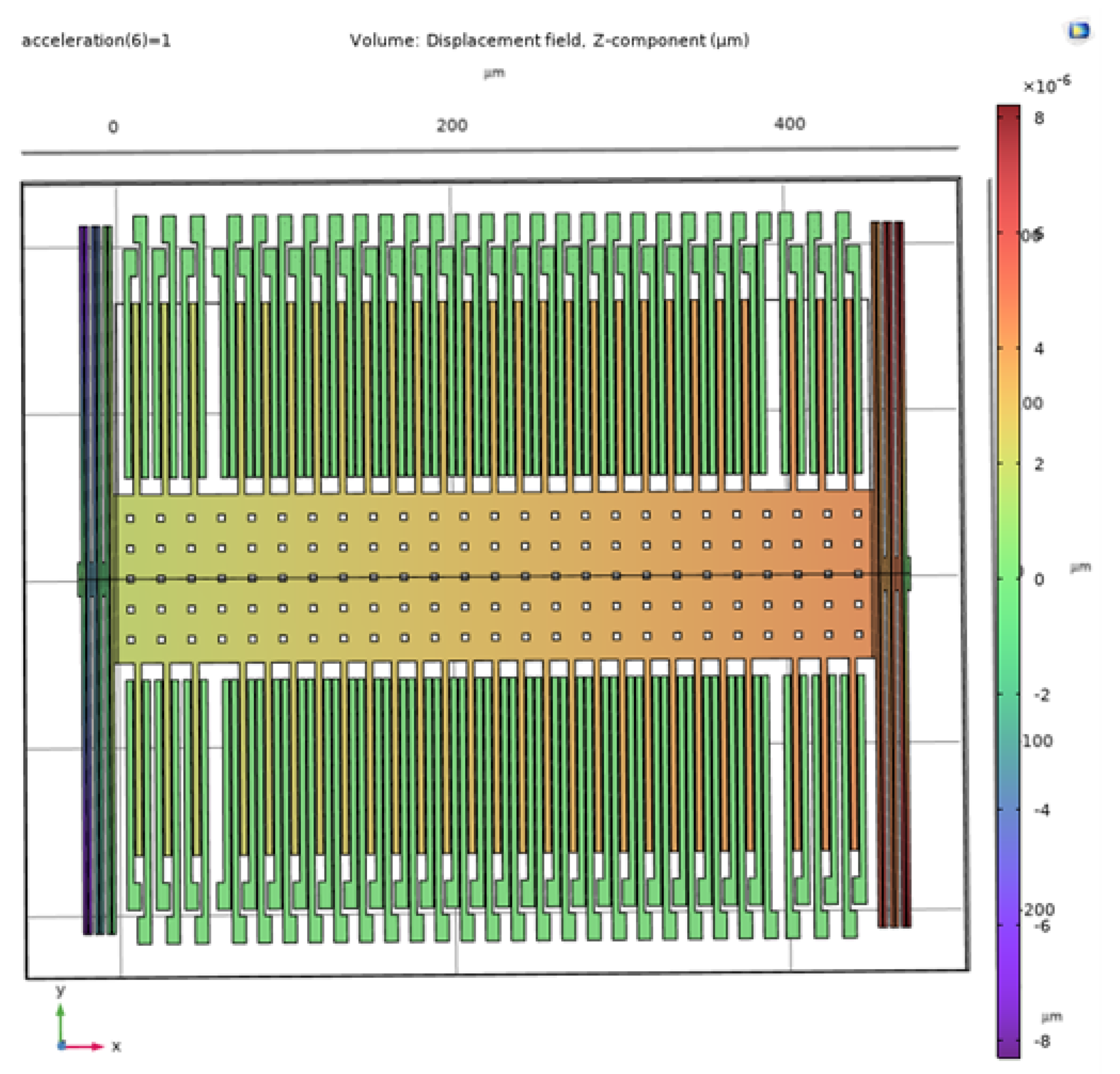
Figure 12.
Sense Voltage vs Acceleration
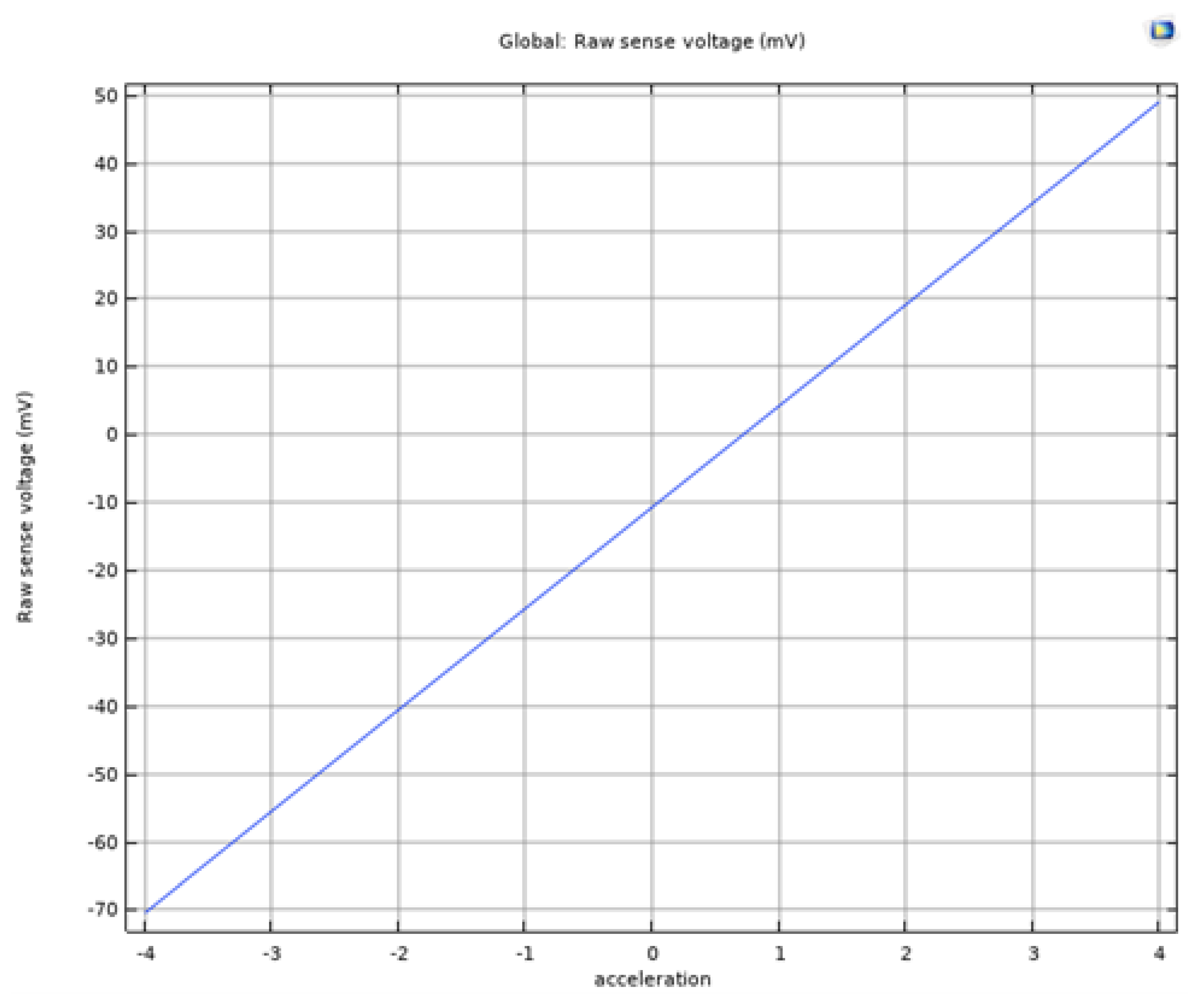
Figure 13.
The COMSOL simulation of eigenfrequency of the accelerometer model, at 4K Hz
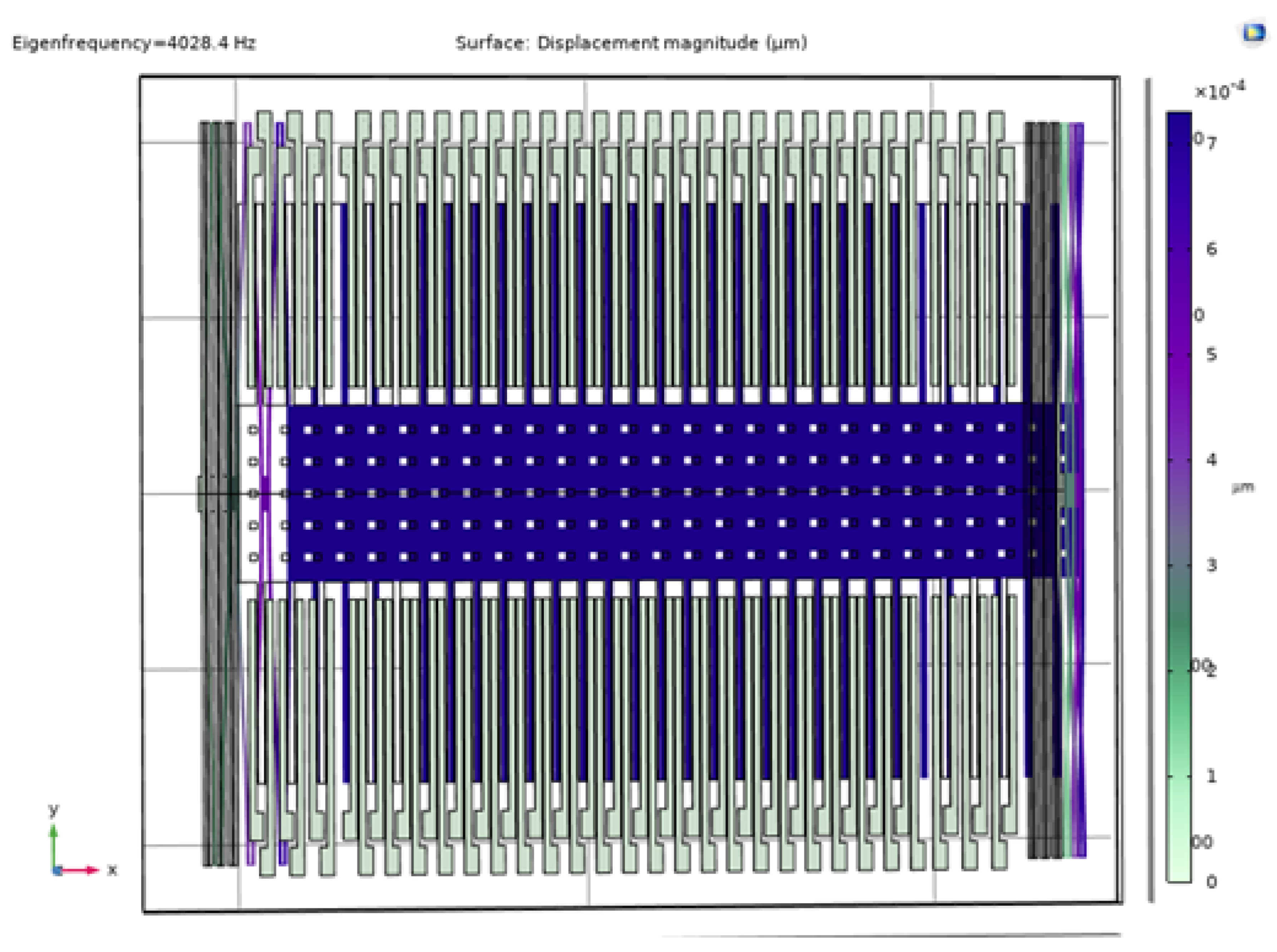
Figure 14.
The COMSOL simulated 2nd eigen frequency - 7K Hz, which shows the out-of-plane defelection of the structure.
Figure 14.
The COMSOL simulated 2nd eigen frequency - 7K Hz, which shows the out-of-plane defelection of the structure.
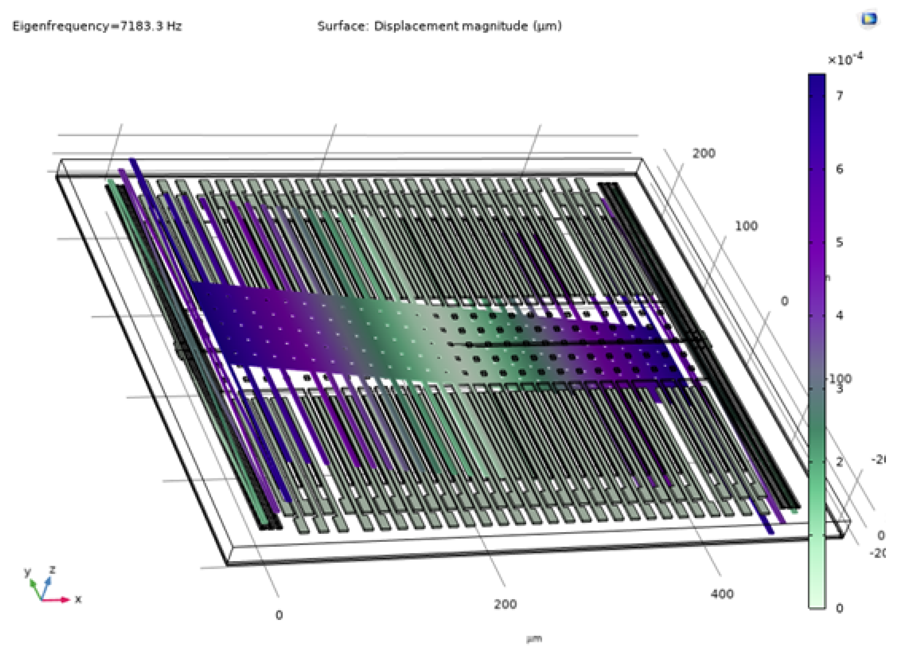
Figure 15.
The stress distribution in accelerometer structure at +4g acceleration, the high stress regions are in the spring structure
Figure 15.
The stress distribution in accelerometer structure at +4g acceleration, the high stress regions are in the spring structure
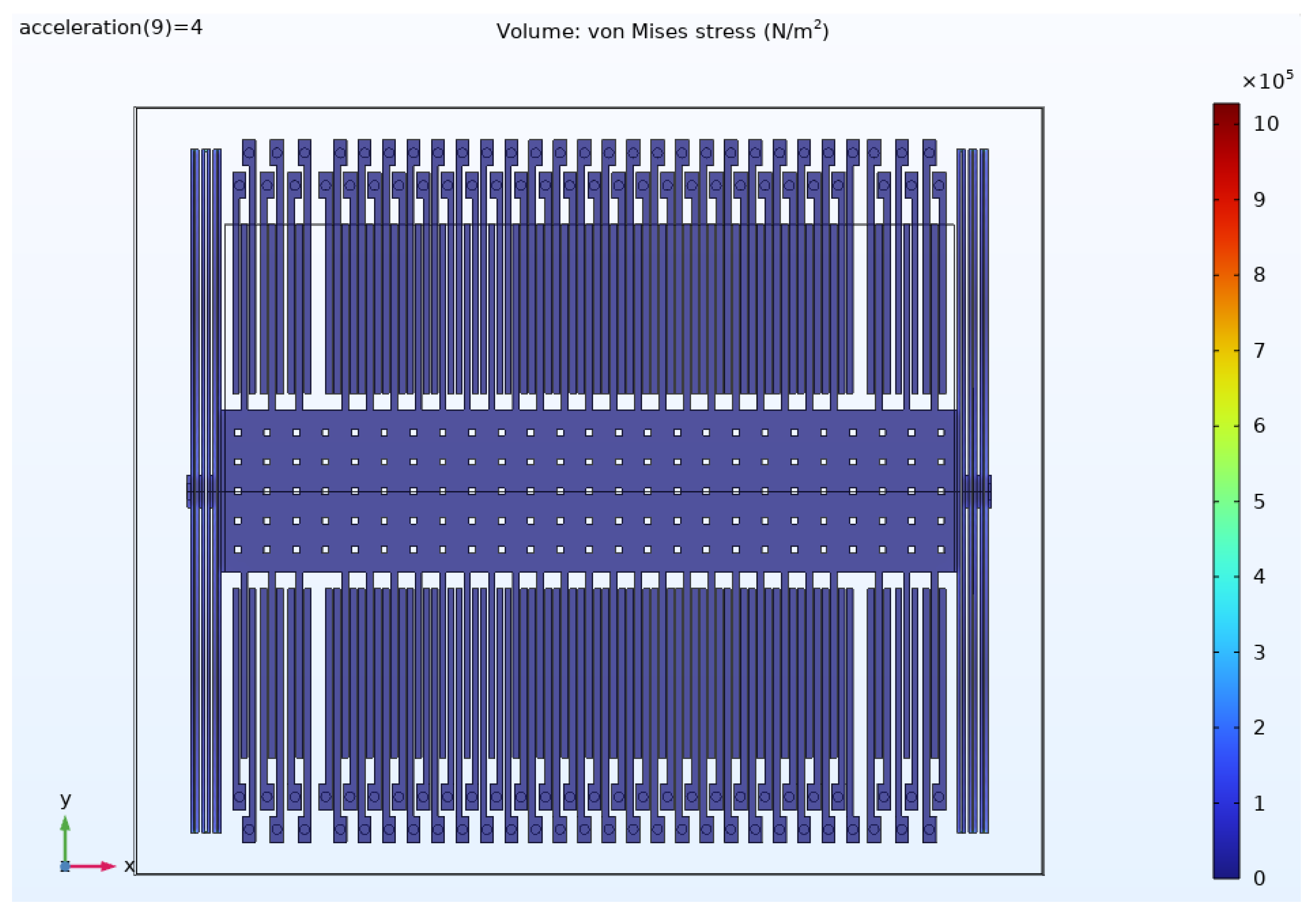
Figure 16.
The enlarged images of spring structure, which shows the high stress regions are at joint sections of the folded beam structure
Figure 16.
The enlarged images of spring structure, which shows the high stress regions are at joint sections of the folded beam structure

Figure 17.
Illustration of Squeeze Film Damping
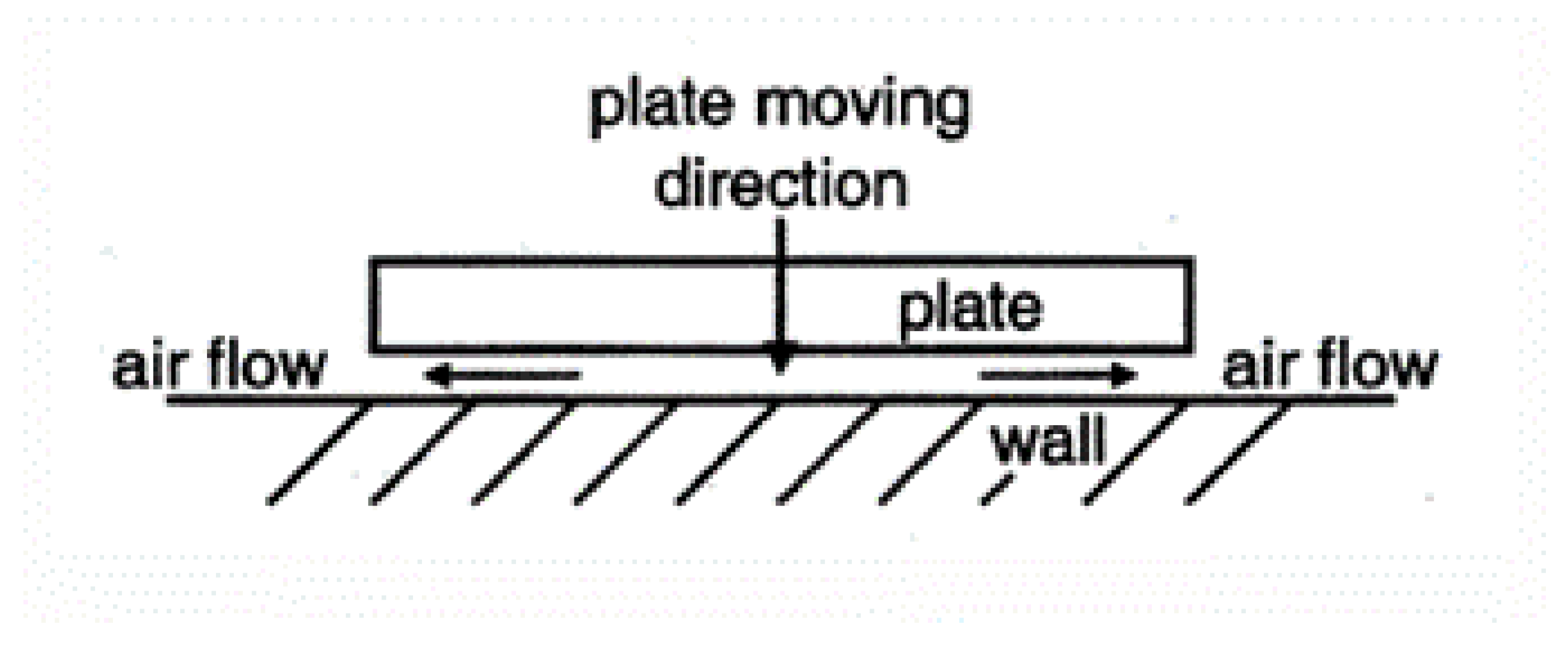
Figure 18.
Gas film pressure with no etch holes
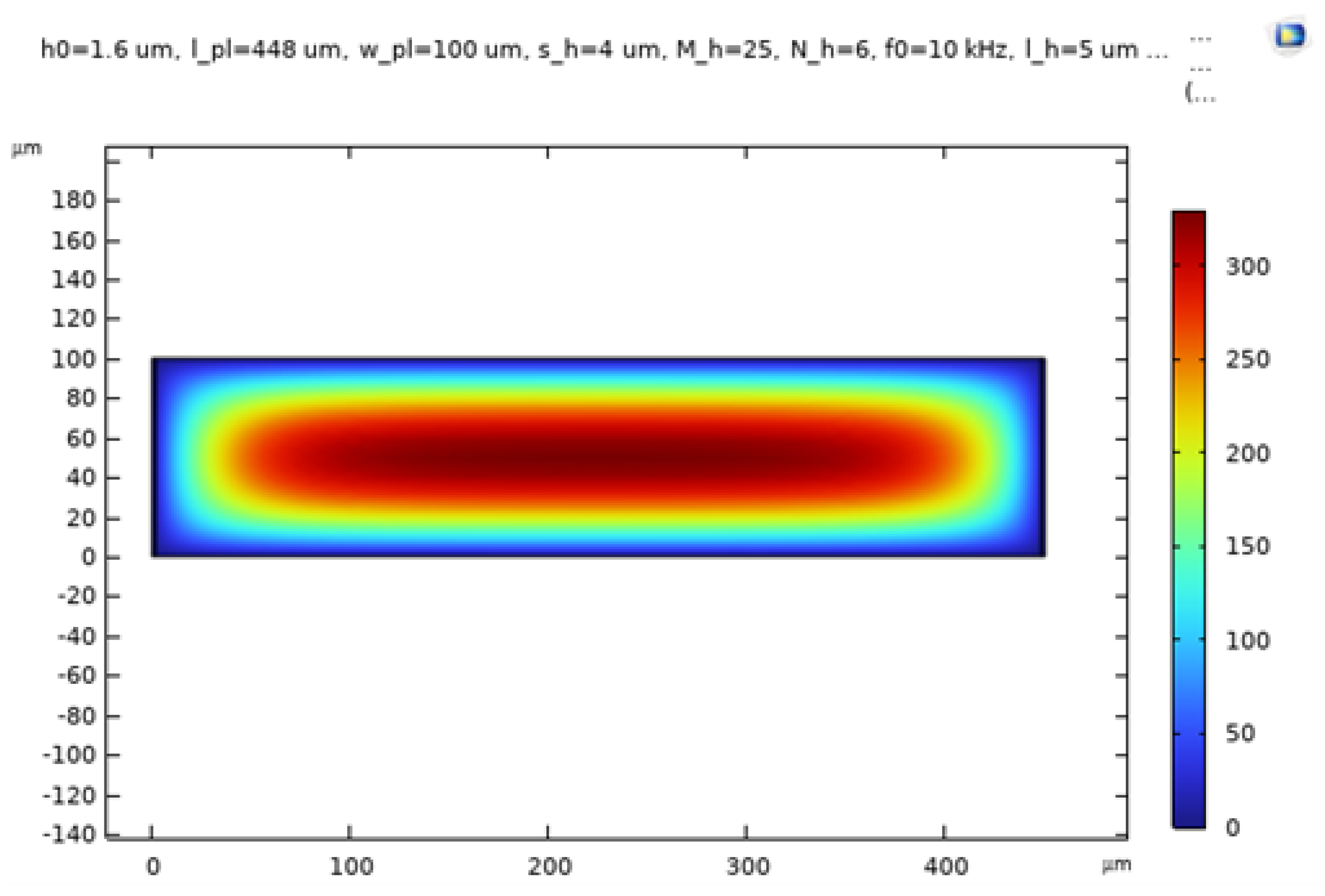
Figure 19.
Gas film pressure with BAO model
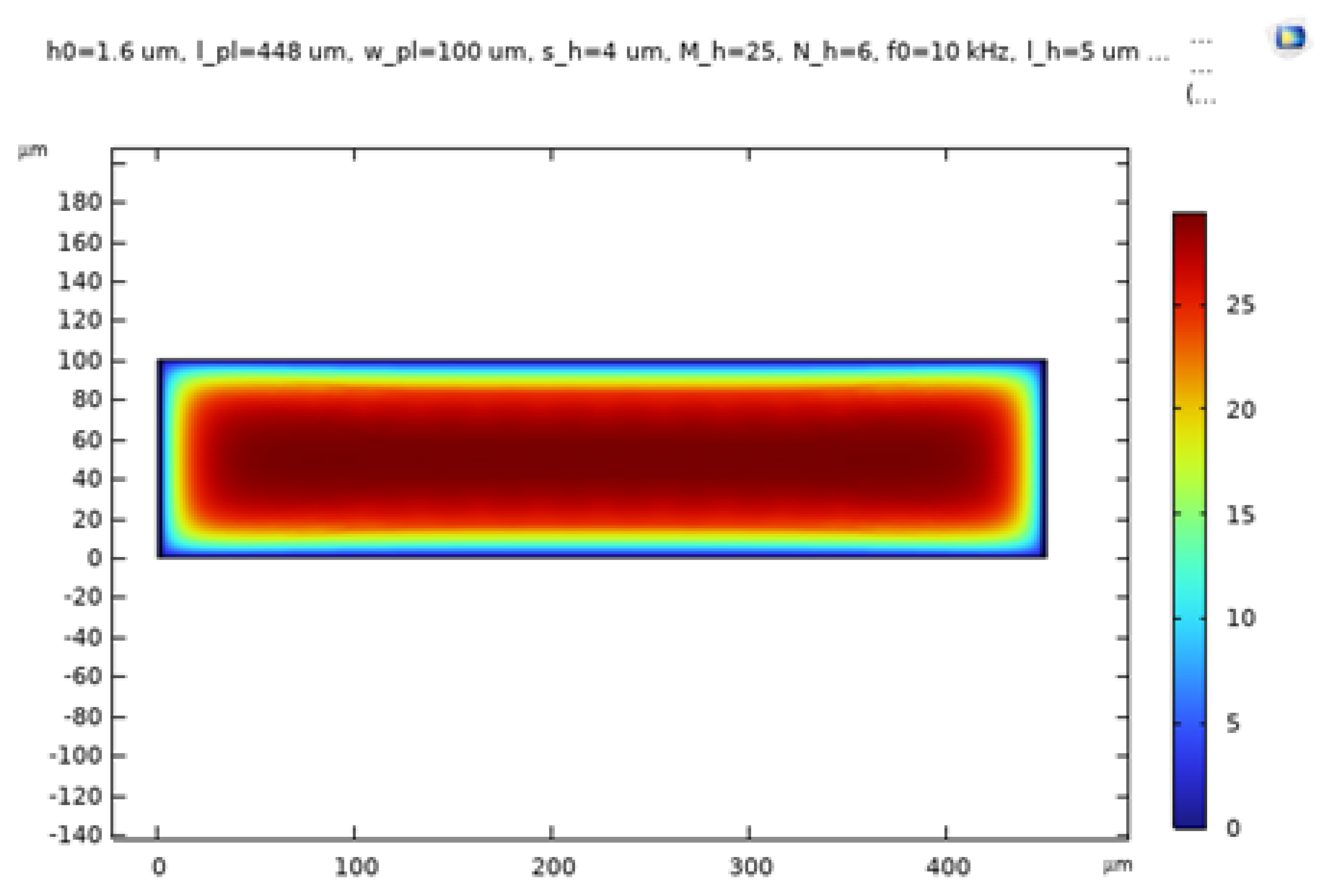
Figure 20.
Gas film pressure with zero pressure and perforations
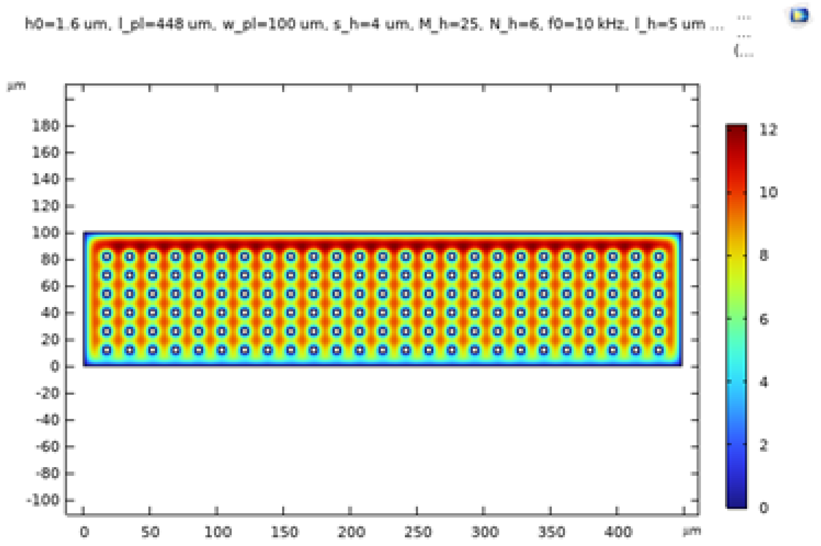
Figure 21.
Comparison of pressure variations at different perforations
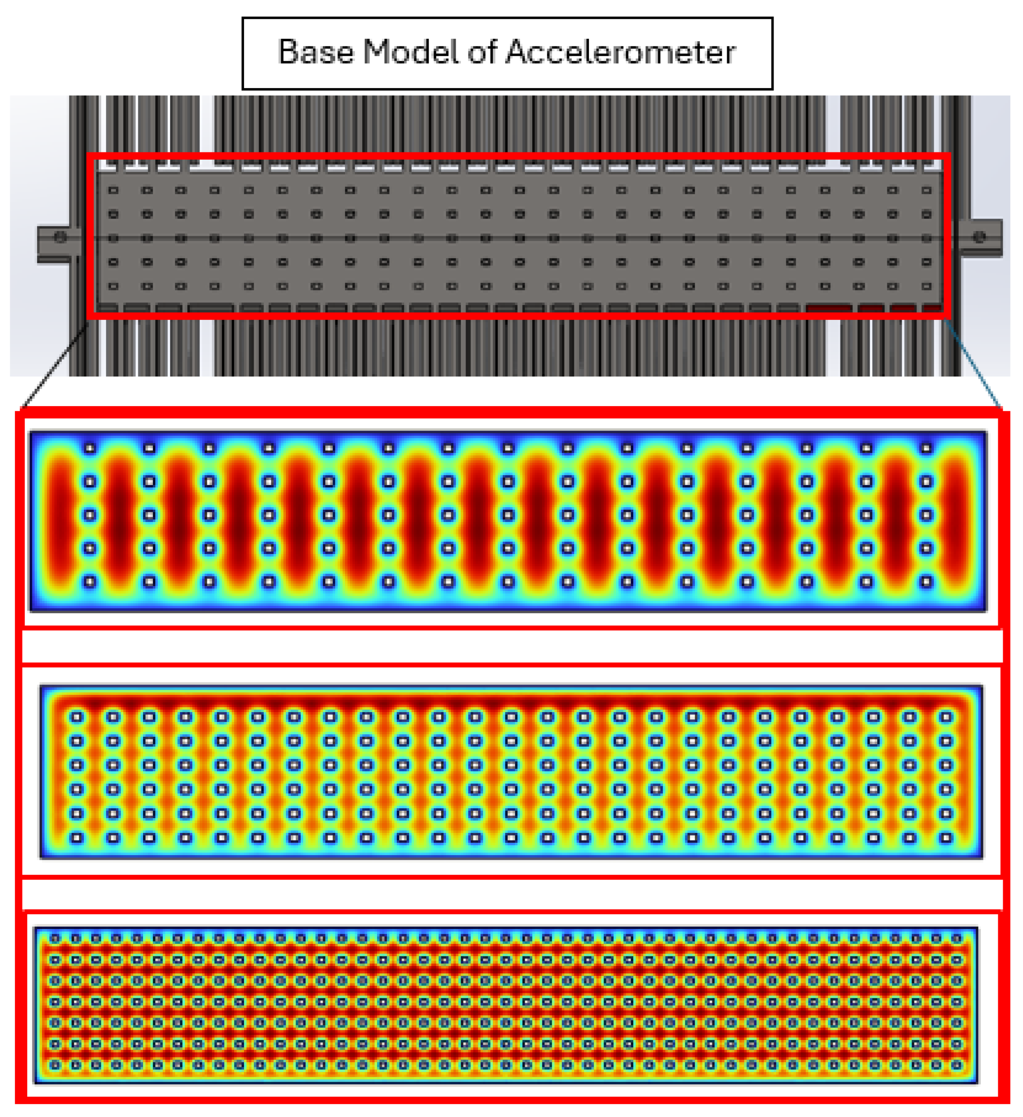
Figure 22.
Damping coefficient for three cases
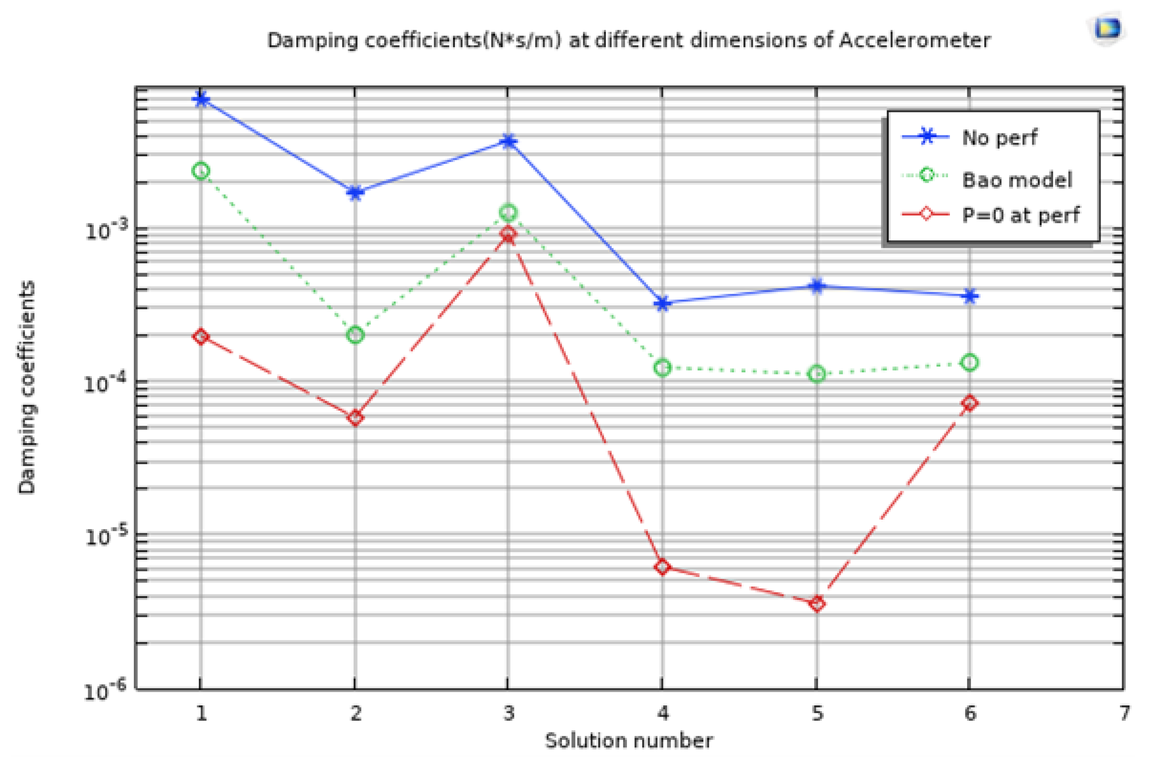
Figure 23.
Sweep Parameters for Squeeze Film Damping
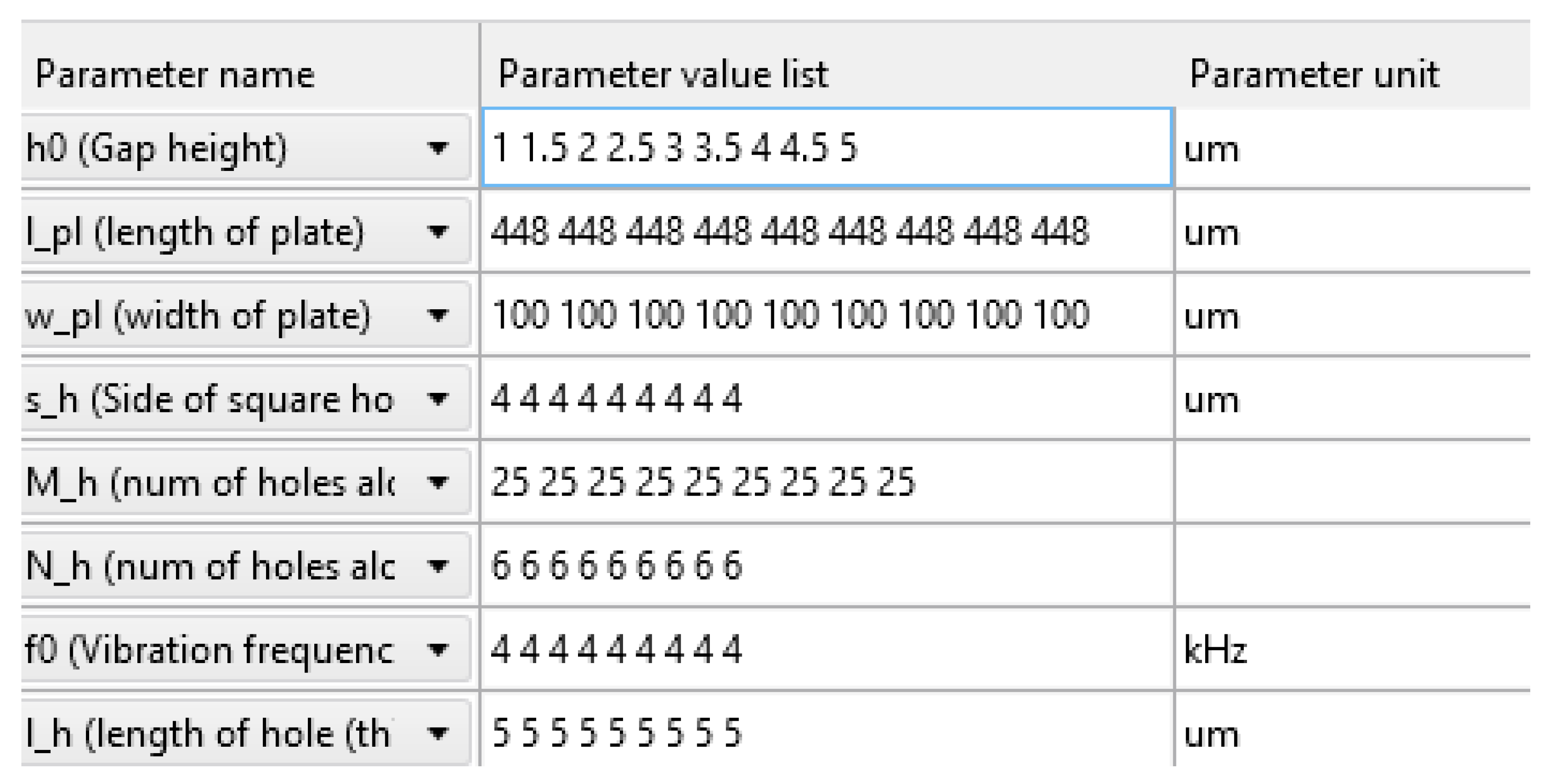
Figure 24.
Final Squeeze Film Damping Coefficient over Height Gap for this Accelerometer
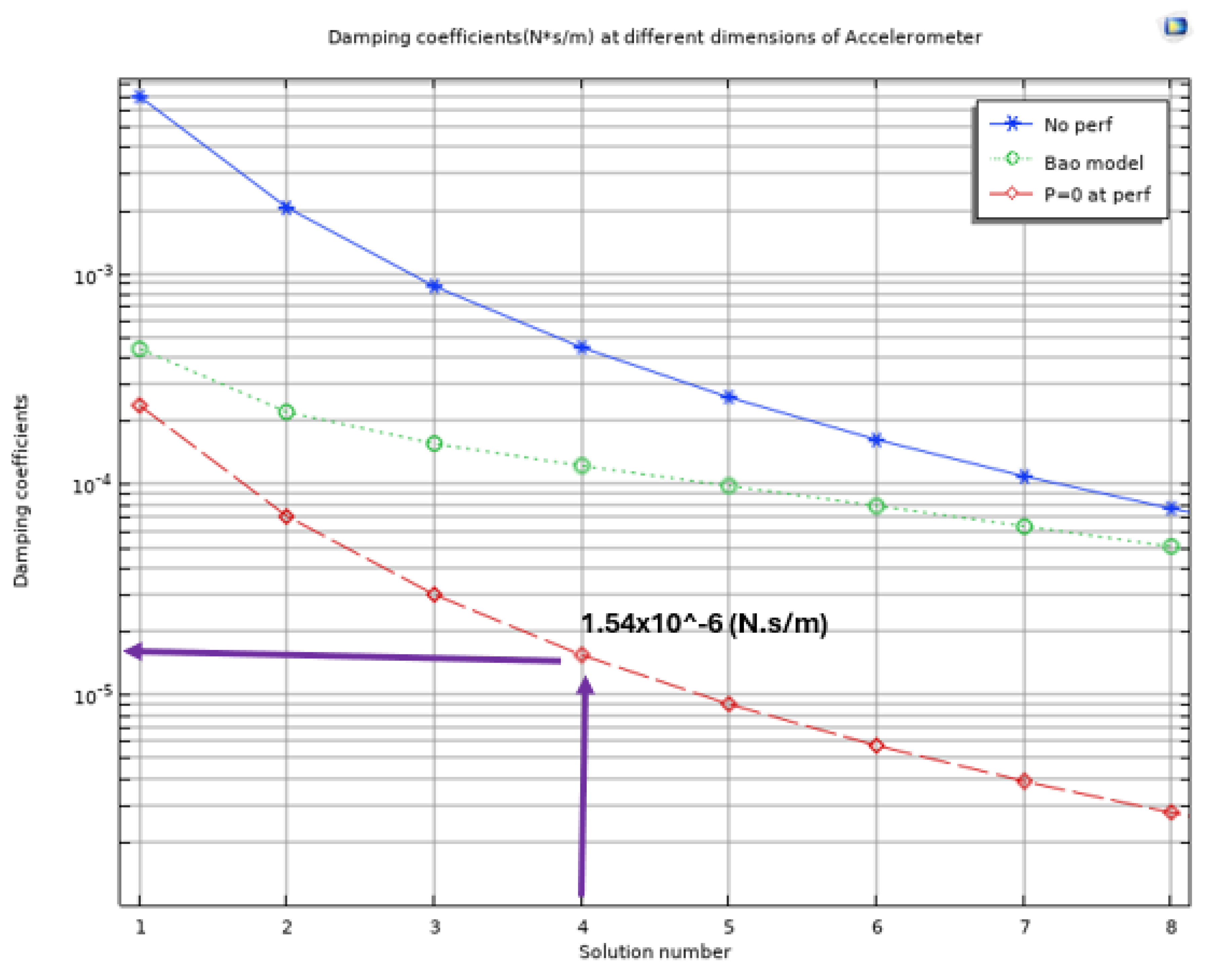
Figure 25.
Frequency Response - Optimum b value calculation
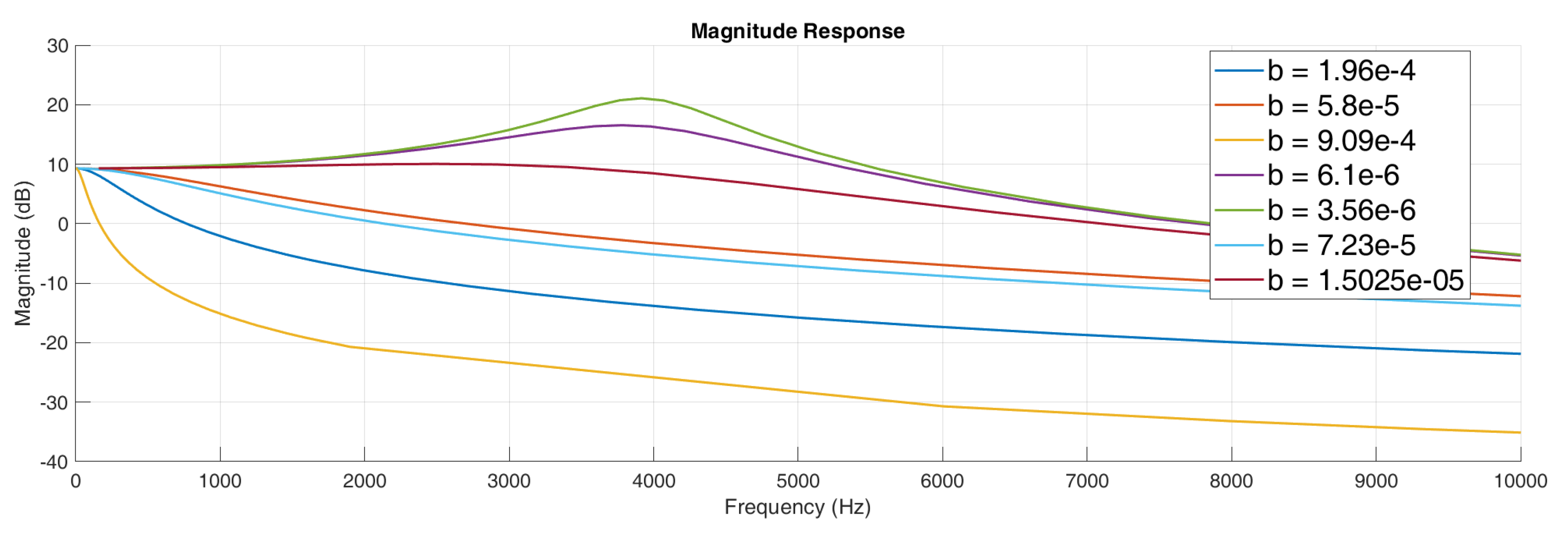
Figure 26.
Frequency response of the accelerometer design
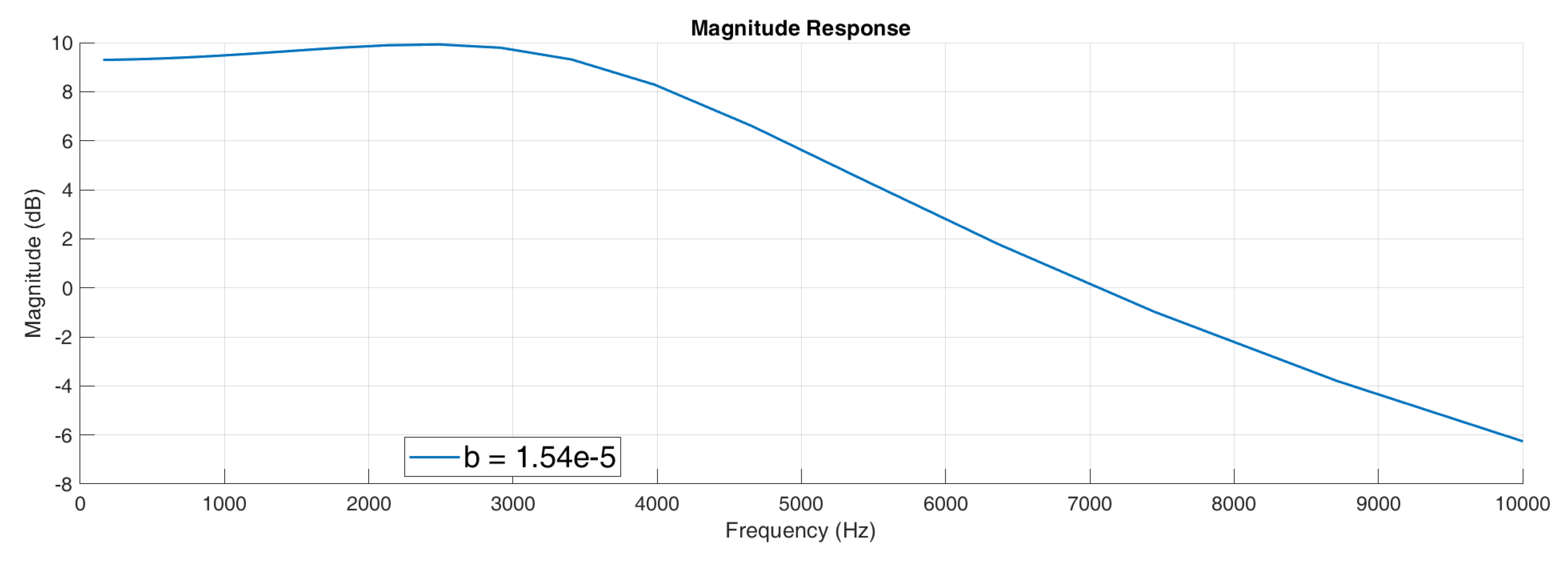
Figure 27.
Lumped Circuit Model
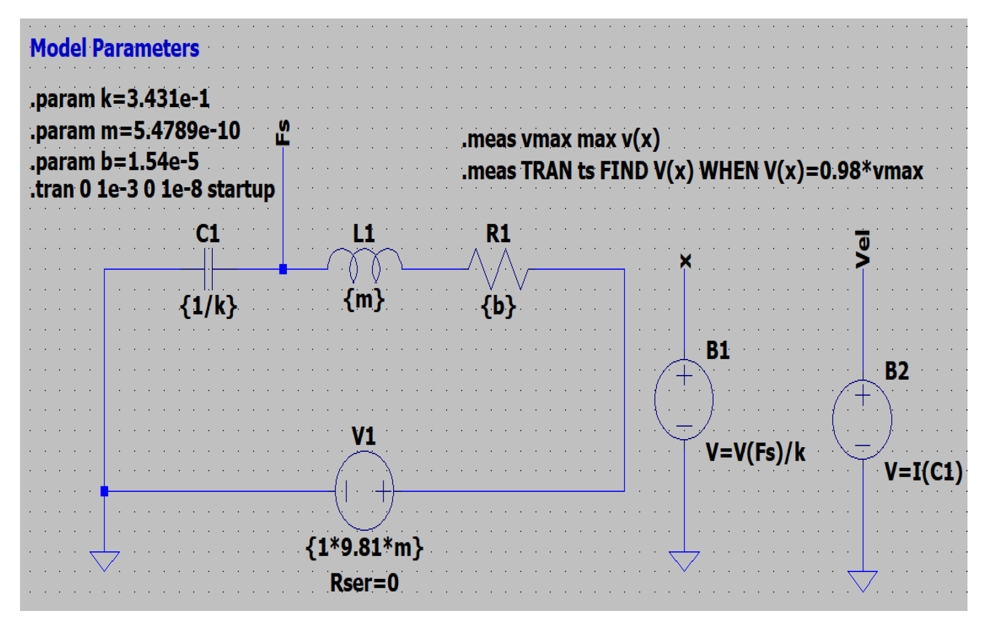
Figure 28.
Position-Time Response
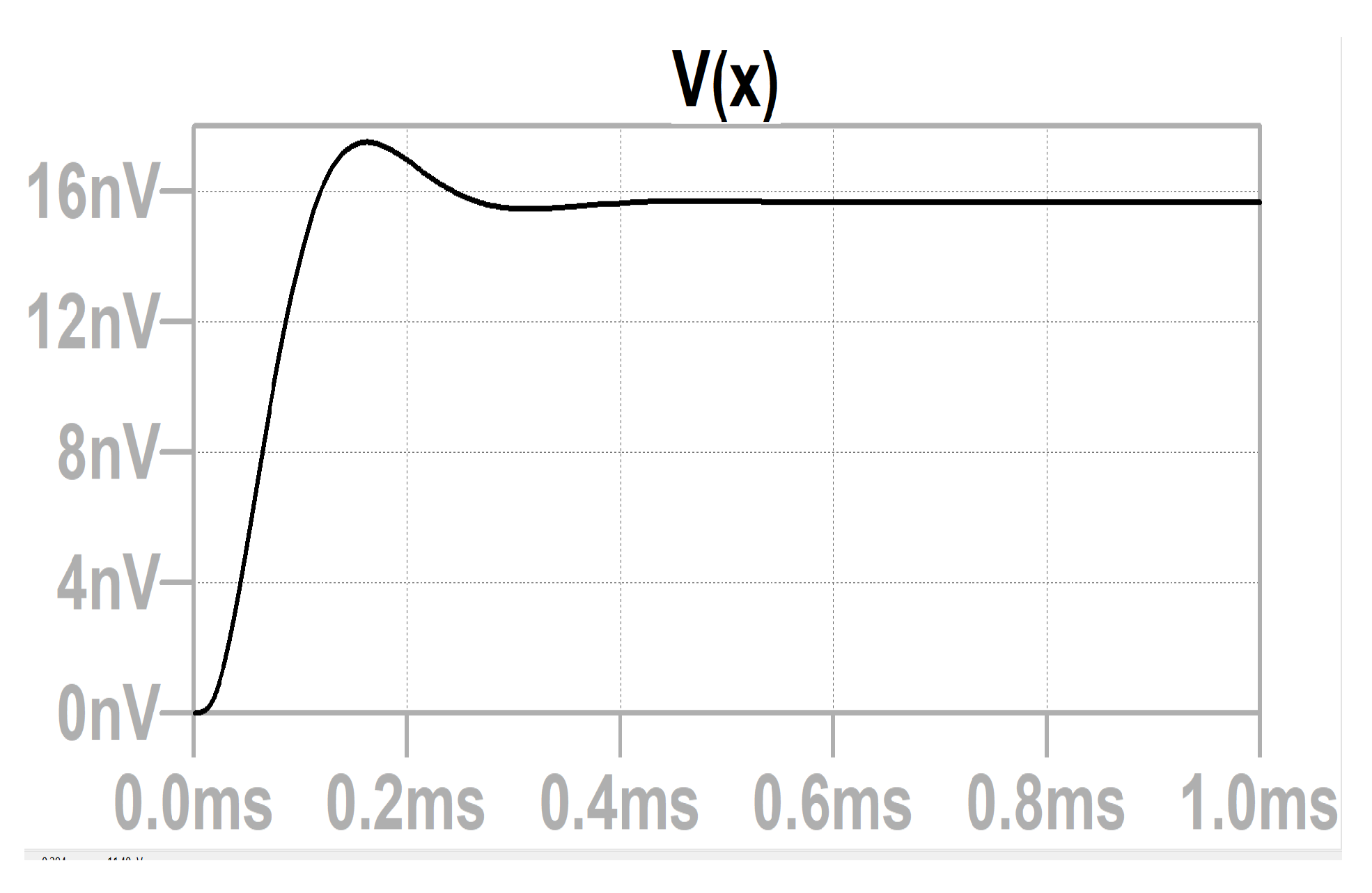
Table 1.
Boundary Conditions for ROM Applications
| Parameter | Specification |
|---|---|
| Temperature Range | -40°C to 85°C |
| Acceleration Range | -4g to 4g (tunable up to 16g) |
| Shock Limit | 10,000g |
| Vibration Limit | 2,000g |
| Mounting Orientation | Lateral |
| Power Supply Voltage | 3.3V to 5V |
| Frequency Response | 10Hz to 1000Hz |
| Initial Operating Pressure | 1 atm |
Table 2.
Meshing Parameters for Model
| Parameter | Value |
|---|---|
| Maximum Element Size | 20.8 m |
| Minimum Element Size | 10 m |
| Maximum Growth Rate | 1.5 |
| Curvature Factor | 0.6 |
| Resolution in Narrow Regions | 0.5 |
Table 4.
Dimensions of the folded beam structure L1 and L2
| No | Spring Constant | L1 | L2 |
|---|---|---|---|
| 1 | k1 | 199 µm | 199 µm |
| 2 | k2 | 199 µm | 159 µm |
Table 5.
Summary of Analytically Calculated Parameter Values and Metrics
| No | Parameters | Value | Remark |
|---|---|---|---|
| 1 | Spring constant - K | 0.2546476 N/m | - |
| 2 | Mass (Movable mass) - M | 5.5002 × 10⁻¹⁰Kg | Per-mass and fingers |
| 3 | Resonance frequency - ωr | 21.5 kHz | |
| 4 | Slip film - Dsl(s | 2.93 × 10⁻⁶ Ns/m | Damping Coefficient |
| 5 | Air Drag - Dad(s | 1.92 × 10⁻⁸ Ns/m | Damping Coefficient |
| 6 | Quality Factor - Q | 0.77 | - |
| 7 | Sensitivity (capacitive) | 4.62 fF/g | ΔC/g |
| 8 | Sensitivity (displacement) | 21.18 nm/g | Δx/g |
| 9 | Sensitivity (sense voltage) | 78.2 | µV/g (5mV) |
| 10 | Brownian Noise | 21.46 ng/√Hz | - |
Table 6.
Dimensions of accelerometer design and physical constants used for Slip film damping coefficient calculation
Table 6.
Dimensions of accelerometer design and physical constants used for Slip film damping coefficient calculation
| No | Parameters | Value | Unit |
|---|---|---|---|
| 1 | Kinematic Viscosity of Air (298 K) | 1.8 × 10⁻⁵ | Pa s |
| 2 | Gas gap - bottom | 2 | µm |
| 3 | Gas gap - top | 5 | µm |
| 4 | Proof mass- Electrode gap | 10 | µm |
Table 7.
Summary of achieved Parameter Values from Simulation
| No | Parameters | Value |
|---|---|---|
| 1 | Sensitivity | 15 mV/g |
| 2 | Full-scale Range | -4g to 4g |
| 3 | Bandwidth | 3000 Hz |
| 4 | Sensor Resonance frequency | 4028 Hz |
| 5 | Self Test Output change | 0 - 2 V |
| 6 | Quality factor - Q | 0.89 |
| 7 | Damping Ratio - ζ | 0.56 |
Disclaimer/Publisher’s Note: The statements, opinions and data contained in all publications are solely those of the individual author(s) and contributor(s) and not of MDPI and/or the editor(s). MDPI and/or the editor(s) disclaim responsibility for any injury to people or property resulting from any ideas, methods, instructions or products referred to in the content. |
© 2025 by the authors. Licensee MDPI, Basel, Switzerland. This article is an open access article distributed under the terms and conditions of the Creative Commons Attribution (CC BY) license (http://creativecommons.org/licenses/by/4.0/).
Copyright: This open access article is published under a Creative Commons CC BY 4.0 license, which permit the free download, distribution, and reuse, provided that the author and preprint are cited in any reuse.


