
Submitted:
21 February 2025
Posted:
25 February 2025
You are already at the latest version
Abstract
In scientific and engineering computations, the efficient solution of partial differential equations (PDEs) is of great significance. This paper proposes an innovative method based on the combination of the U-Net neural network and the Fourier neural operator, aiming to improve the accuracy and efficiency of solving PDEs. The unique encoder-decoder structure and skip connections of the U-Net neural network can effectively extract and integrate spatial domain features, accurately depicting the spatial structure of PDEs. The Fourier neural operator, by means of the Fourier transform, deeply explores and processes features in the frequency domain, capturing the frequency characteristics of the solutions of PDEs. By organically combining the two, this method not only preserves spatial details but also makes full use of frequency domain information. It significantly reduces the model's dependence on large scale data and enhances its generalization ability. Experimental results show that compared with traditional methods, this method performs outstandingly in various complex partial differential equation(PDE) solving tasks, achieving higher accuracy. It provides a new and highly promising solution for the solution of PDEs and is expected to be widely applied in related fields.
Keywords:
neural operator
; Partial differential equation
; U-Net
; Fourier transform
1. Introduction
In fluid mechanics, geophysics, biology, and many other fields, the partial differential equation (PDE) model serves as a crucial tool for characterizing various phenomena. Related problems encompass physical model building, the solution of partial differential equations, and parameter inversion. The process of solving a partial differential equation involves obtaining a spatially accurate solution or a numerical solution under the known partial differential equation and other constraints [1,2,3,4].
Traditional numerical solution methods for partial differential equations rely on discrete scheme based finite difference systems, commonly referred to as the computational fluid dynamics method (CFD). Examples include the Runge-Kutta method, the prediction correction method, the finite element method [5], the finite difference method [6], and the finite volume method [7], among others. In contrast to traditional solving methods, neural networks exhibit distinct advantages in solving differential equations. Neural networks possess a powerful data fitting capacity, and even a small scale neural network can handle simple partial differential equations [8]. Employing the neural network approach to solve differential equations effectively addresses issues such as poor adaptability and conditional limitations of grid sections. Compared with traditional numerical methods, the neural network method requires fewer sampling points to achieve higher accuracy. Moreover, once a neural network model is trained, it can be directly utilized to calculate the numerical results at any point within the obtained domain. Since the 1990s, some scholars have initiated research on the mathematical foundations and methods of using neural networks to solve differential equations. In 1990, Hornik et al. [9] demonstrated that under certain conditions, a multilayer neural network can approximate any function and its derivative, even when the function only has a generalized derivative. This finding laid the groundwork for neural network based solutions to partial differential equations. In 1998, Lagaris and Likas [10] put forward a method for solving the first boundary value problem using an artificial neural network (ANN). In 2011, Kumar and Yadav [11] investigated multilayer neural network (MLP) and radial basis function neural network (RBF) models for solving differential equations, and compared and summarized the applications of MLP and RBF in this regard. In 2018, Winovich et al. [12] proposed a quantitative uncertainty convolutional neural network (ConvPDE-UQ) for the problem of heterogeneous elliptic partial differential equations on different domains. Also in 2018, Long and Dong et al. [13,14] introduced a novel feed forward neural network (PDE - Net). Its core concept is to approximate the differential operator with a convolution kernel, construct a network to approximate the nonlinear partial differential equation system, and achieve long term prediction of its solution. A convolutional network is essentially an input to output mapping, capable of learning numerous mapping relationships between input and output without the need for any precise mathematical expressions between them. However, due to the increase in dimension, the solution accuracy of the convolutional neural network model [15] is slightly diminished. Most of the above mentioned neural network based methods for solving partial differential equations are focused on the initial boundary value problem. The network takes space coordinates or time variables as inputs and outputs the solution values in space. When constructing solutions by integrating partial differential equations with neural networks, the optimization objectives typically consist of two parts: the errors at the initial - solution and boundary value sampling points, and the errors at the sampling points within the domain subject to the differential equation constraints.
In addition, when we need to rapidly obtain accurate solutions for a set of partial differential equations, one approach we can adopt is the neuronal operator method. This method can be learned based on the mapping from the source-term function to the solution function of the partial differential equation set [16].
The Fourier transform holds a significant position in deep learning models. It aids in the proof of the universal approximation theorem [17] and can also accelerate the training of convolutional neural networks [18]. Keivan Alizadeh Vahid et al. [19] proposed extending the butterfly operation in the traditional fast Fourier transform and applying it to the design of convolutional neural network architectures. They demonstrated that the computational complexity of the alternative network layer through butterfly transformation was reduced from N to . Experiments also confirmed that the proposed scheme effectively enhanced the model’s accuracy. Integrating the Fourier transform into the neural network model can effectively decrease the model’s computational complexity. Moreover, the physical trends in the data can be effectively captured through the Fourier transform, which offers great advantages for solving partial differential equations. Li [20] proposed the neural operator method, which can be evaluated at any point in time and in any space. Additionally, a general approximation theorem for neural operators was summarized and proven. Li [21] put forward the Fourier neural operator, where the integral operator operates directly in the Fourier space through parameterization. Evidently, the neural operator approach is a fully data-driven method, necessitating a large number of high-quality datasets. However, in the analysis of complex physical, biological, or engineering systems, the cost of data acquisition is often prohibitively high. As a result, we inevitably encounter the challenge of drawing long-term conclusions with partial information, making these methods inefficient. Kushnure et al. [22] proposed an architecture named MS U-Net for multi-scale feature representation and recalibration. This architecture uses the Res2Net module to retain the contextual information of segmented objects, and it squeezes and motivates the network to recalibrate multi-scale feature channels, thereby enhancing the network’s ability to describe high-level features. In the literature [23], for the same data preprocessing, the feature representations of each modality learned by the network are fused at later stages. In the last layer of convolution, a larger-scale feature map is connected to achieve the communication of contextual information between feature maps of different sizes.
This integration of multi-scale feature representation and recalibration mechanisms allows the network to better capture both local and global information, which is crucial for solving complex partial differential equations. By leveraging these advanced techniques, the model can achieve higher accuracy and efficiency in solving PDEs, even in scenarios where data is limited or incomplete.
In summary, the combination of Fourier transforms, neural operators, and multi-scale feature recalibration provides a powerful framework for solving partial differential equations. These methods not only reduce computational complexity but also enhance the model’s ability to capture physical trends and high-level features, making them highly effective for a wide range of applications in science and engineering.
The model extracts information features in the frequency domain through Fourier transform, capturing the key information of the equations, and utilizes convolution neural networks to extract the high-level internal features of the system. By employing a connection-based mechanism for reducing the number of network layers, the model can efficiently solve partial differential equations (PDEs) from both the global and internal characteristics of the system. U-Net extracts image features in the form of convolution, whose essence lies in computing the derivatives of image pixels to capture the variations in the image. On the other hand, the Fourier neural operator calculates derivatives in the form of filter operators, enabling rapid computation through convolution functions.
Building on this foundation, this paper proposes a Fourier neural operator-based U-Net neural network model. This model approximates higher-order differential operators using multiple low-order constrained convolution kernels, thereby better characterizing the properties of the differential equations. In the model design, the feed forward neural operator serves as the core component, containing tunable parameters that can be continuously optimized through training. This design not only enhances the model’s solving accuracy but also supports long-term stable numerical solutions, as validated by experimental results.
2. Preliminaries
2.1. Parametric Partial Differential Equations
Let G be the nonlinear operator, general parametric PDEs can be expressed as: .
Where u is the input function, and s is the solution to an unknown partial differential equation (and also a function).
Our PDE solution operator will be .
We can express the general solution of our PDE as the operator .
A common instantiation is the approximation of the second order elliptic PDE:
Where u is our target solution object, is the right end term, which is regarded as a forcing term in many physical equations, and this is the parameter, , where is the parameter space. If we write it in the form of the operator, we express it in the following form
Where , the subscript a means the operator at the parameter a.
Under rather general conditions of , we can define the Green function as the unique solution to the problem:
To be concrete we will consider infinite-dimensional spaces which are Banach spaces of real-valued functions defined on a bounded open set in . We then consider mappings which take input functions to a PDE and map them to solutions of the PDE, both input and solutions being real-valued functions on .
2.2. PDE Setting
Let and U be separable Banach spaces and a (typically) non-linear map.
For some bounded, open domain and a fixed source function f. For a given function a, the equation has a unique weak solution u, so we can define the solution operator as the map of the function to the function.
Our goal is to learn an operator to approximate by using a limited set of observed input-output pairs , where each and are a function on D.
We aim to build an approximation of by constructing a parametric map
for some finite-dimensional parameter space and then choosing so that .
So our optimization problem goal is the minimization problem of the loss function
which directly parallels the classical finite-dimensional setting.
This is an example of a quote.
3. Algorithm
3.1. Setting of Input Signal and Function Space
The input signal serves as the key factor for a model to gather characteristic information, and its quality sets the upper limit of the model’s achievable accuracy. In this paper, we primarily consider two function spaces:
The Orthogonal (Chebyshev) Polynomial Component of the Gaussian Random Field (GRF) and the Gaussian Random Field (GRF).
Typically, we employ a zero - mean Gaussian random field, expressed as:
where the covariance function is the Gaussian kernel given by:
The length scale l here is of great significance as it determines the smoothness of the sampling function. When the value of l is large, the resulting u function will be smoother, which is of great importance for studying phenomena at different scales.
After selecting the function space, sampling needs to be carried out from this space. The specific approach is to scatter points within the specified region to obtain sample points. Subsequently, the is integrated, and the resulting value is used as the input data of the model. By constructing the model in this way, an approximate solution y is obtained. To comprehensively evaluate the performance of the model, multiple different test sets u are generated by randomly selecting data, so as to examine the performance of the model under different data distributions.
Gaussian random field with the radial-basis function kernel:
Suppose there is a stochastic process that follows a specific Gaussian random field distribution, that is:.
Then, can be represented by the following integral from:
In the above expression, W and B are independent standard Brownian motions, which introduce randomness to . To further simplify the expression, a variable substitution is carried out, apply the change of variable and. After the transformation, can be rewritten as:
Applying a linear interpolation on the interval , then
where we recalled the error estimate of the linear interpolation on (by Taylor’s expansion)
where lies in between a and Then by the Borel-Cantelli lemma, we have
where C is an absolute value of a Gaussian random variable with a finite variance. Therefore, taking a piecewise linear interpolation of with m points will lead to convergence with order
3.2. Structure Based on U - Net Neural Network and Fourier Neural Operator
The U-Net neural network, as a classic deep-learning architecture, has a unique structure. The first half is mainly responsible for feature extraction, while the second half focuses on the up-sampling operation. This structure is called the encoder-decoder structure. In this study, a Fourier neural operator with adjustable parameters is introduced. By skillfully integrating the feature information extracted by the U-Net neural network into the Fourier operator, the operational efficiency and solution accuracy of the algorithm can be significantly improved.
Step1: When constructing the algorithm framework, P and Q are defined to represent the left - contracting path and the right-expanding path of the U-Net neural network respectively:
Among them, represents the number of channels used in the neural network. Usually, the value of is greater than or . In the actual operation, the left - contracting path P of the U-Net is used to lift the input data to a high-dimensional channel space, and then the right - expanding path Q is used to project the data in the channel space to the final output space.
The left encoder network P has a structure similar to that of a convolutional neural network. For a given input function a: , its operation process includes two repeated convolution operations, a rectified linear unit (ReLU activation function), and a max-pooling layer. When performing the down-sampling operation, the algorithm step size is set to 2.
Convolutional layer:
. Where is convolution operation, W is convolution kernel and b is bias.
ReLU activation functions:
Pooling layer: The maximum pooling layer is usually used to reduce the spatial dimension and help to obtain. Enter the features of the image:
Input a into the encoder (left-contracting path P) of the U-net neural network. Through convolution, ReLU activation function, and max-pooling layer operations, the input is lifted to the high dimensional channel space .
Step2: Then we introduce the nonlinear integral Fourier operator
Apply four-layer integral operators and activation functions to the obtained feature , and update it specifically according to the formula
Where is an activation function is a linear transformation. It can handle lower Fourier patterns and filter out higher patterns, and into the nucleus to , this is all something to learn from the data. Step3: The resulting result is again input into the U-Net neural network decoder Q, deconvolved, jump connections, and other operations, which help to retain high-resolution details.
Similar to the encoder, the decoder also applies the convolution and activation functions to handle the feature graph.
Input the updated result into the decoder (right-expanding path Q) of the U-net neural network. Process it through operations such as de-convolution and skip connection, and finally output .
Step4: The final output results and the original sample to calculate the loss through the loss function, and finally through the loss function to optimize the U-Net network and the Fourier operator to obtain the optimal parameter value.
Where
Here, represents the initial and boundary training datasets. The loss term corresponds to constraints imposed by the initial data and boundary data.
Here, the set represents the collocation points for , with the loss function enforcing the structural constraints imposed by equations.
Optimize the parameters of the U-Net network and the Fourier operator through the loss function to obtain the best parameter values and minimize the loss.
Figure 1.
The architecture of the neural operators.
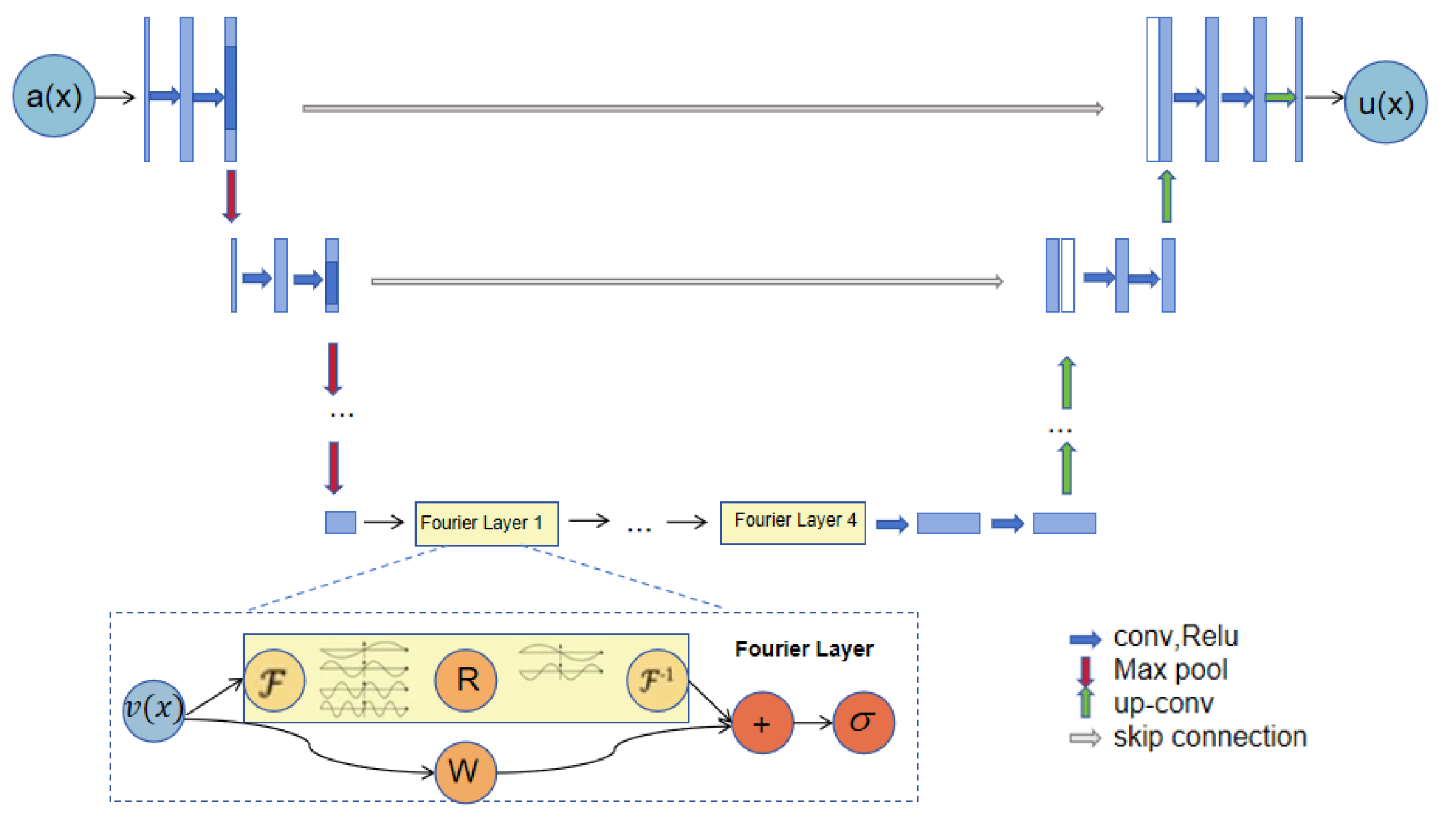
The complete structure of the neural operator: The entire operation process of the neural operator starts from the input a. First, the input data is upgraded to a high-dimensional channel space through the U-Net encoder. Then, four layers of integral operators and activation functions are applied to deeply process the data. After that, the processed data is sent to the target dimension through the U-Net decoder, and finally, u is output.
Fourier layer: The operation of the Fourier layer starts from the input . First, the Fourier transform is applied to transform the data into the frequency domain. Then, a linear transformation R is performed on the low-frequency signals to filter out the high-frequency signals. After that, the inverse Fourier transform is applied to transform the data back into the time domain. At the bottom, a local linear transformation W is also applied to further process the data.
The above formula can be seen as a combination of a linear connection and a nonlinear transformation, and then through the activation function.
The nonlinear transformation is implemented through a kernel integration operator:
The choice kernel form is , the above operation is formally similar to the convolution operation, so it can be expressed by the Fourier transform:
A parameter matrix is introduced, which can transform the lower Fourier patterns and filter out the higher patterns.The Fourier neural operator is finally expressed as follows:
Where , , is both of A function space.
4. Experiment
This section mainly uses the UNO model to solve the 1-d Burgers’ equation, the 2-d Darcy Flow equation and the 2-d Navier-Stokes equation. First, we introduce the experimental configuration and the experimental parameter settings. Then explain the experimental effect section. Finally, solve the partial differential equation according to the model framework introduced and proposed in this chapter, comparing the merits of this model for solving partial differential equations, we get the solution speed, the solution result, and the error with the real solution of the model in the three equations.
4.1. Burgers
In this paper, we choose the 1-d Burgers equation, which is a nonlinear partial differential equation. The equations considered in this paper are as follows, formally:
Where is the unknown function, which depends on the time variable t and the spatial variable x, is the viscosity coefficient, the initial condition is , and the boundary condition is the periodic boundary condition.
According to randomly sampling , modes = 16, width = 64, batch size=20. Forced term =0, viscosity coefficient , grid , other grids directly subsampled. Network input , output , we have 8192 in 2048 grid samples, here is the average sampling, neural network input dimension (20,128,2), input neural operator dimension after dimension (20,128,64), the accuracy of the equation label determines the model accuracy, if the label accuracy is poor, the model has no sense.
The approximate solution is u, and the true solution is uacc, with an error of , . The solver is GPU, the error is , G training label is approximate solution.
It is expected that any f=net (x,y) has G (f, x, y) satisfying the solution constraint regularization of the corresponding PDE.
Figure 2 randomly intercepts several algorithm results from different periods, showing the error between the prediction and the true value of the algorithm, without much change to the naked eye, and the visualization effect is good.

Table 1.
Experiment 1 results.
| Network | s=64 | s=128 | s=256 | s=512 | s=1024 | s=2048 | s=4096 | s=8192 |
|---|---|---|---|---|---|---|---|---|
| MGKN | 0.0187 | 0.0223 | 0.0243 | 0.0355 | 0.0374 | 0.0360 | 0.0364 | 0.0364 |
| GKN | 0.0392 | 0.0325 | 0.0573 | 0.0614 | 0.0644 | 0.0687 | 0.0693 | 0.0714 |
| PCANN | 0.042 | 0.0391 | 0.0398 | 0.0395 | 0.0391 | 0.0383 | 0.0392 | 0.0393 |
| FCN | 0.0827 | 0.0891 | 0.1158 | 0.1407 | 0.1877 | 0.2313 | 0.2855 | 0.3238 |
| GCN | 0.3211 | 0.3216 | 0.3359 | 0.3438 | 0.3476 | 0.3457 | 0.3491 | 0.3498 |
| FNO | 0.0024 | 0.0063 | 0.0063 | 0.0066 | 0.0048 | 0.0060 | 0.0069 | 0.0024 |
| UNO | 0.0021 | 0.0032 | 0.0020 | 0.0023 | 0.0045 | 0.0021 | 0.0060 | 0.0018 |
Figure 3 compares the errors as the number of iterations increases when the subsampling rate varies. Moreover, we can see that when the subsampling rate is 3 and 5, the error is minimized and the algorithm is better than other cases. It can be seen from the algorithm comparison diagram on the right of Figure 3 that the different algorithms exhibit the ability to solve the partial differential equations in the one-dimensional Burgs equation experiment. The UNO model uses convolution to extract physical feature information. The jump connection reduces the information loss of the model. The results are more accurate and smaller than other algorithms, which is better than other algorithms.
4.2. Darcy Flow
In this paper, we choose the steady-state 2-d Darcy flow equation for a second-order linear elliptic partial differential equation.
Where the boundary condition is the Dirichlet boundary condition, a is the diffusion coefficient, , is the solution, and the external force .
We processed the dataset, first is a probability measure with zero Neumann boundary conditions on LaPraaca, where . The external force is fixed to be . The coefficient was sampled from , and the solution u was obtained using the traditional finite element method on the and grids in Matlab. Datasets with different resolutions can be generated by downsampling. We parameterize a two-dimensional Fourier neural operator consisting of four Fourier layers, with 20 frequencies per channel, width = 64.
The loss function can be written in the following form:
In the experimental section, the FNO model, ResNet model, TFNET model, and UNO model were used to solve the 2-d Darcy flow equation.
The true and model solutions of the equations and their errors are shown in Figuer:
Figure 4 shows the contrast between the true and predicted values from 1s to 5s and the error situation, which can be seen per second.
Figure 5 left figure shows that the number of Fourier neural operator layers is different. When the number of Fourier neural operator layers is 1, it takes the least time and the test error is the largest. When the number of levels increases, the time-consuming number increases, but the test error becomes smaller. According to the need, three or four and five layers are the most reasonable, depending on the situation, here take four layer Fourier operator. The right image introduces the effect of the different number of Fourier neural operator layers and the filtered models on the algorithm error as the number of iterations increases. As the number of iterations increases, the error becomes smaller. When the four-layer Fourier neural operator and the filtered out movies are 24, the effect is better and the performance is better. Then the algorithm model selects the four-layer Fourier neural operator.
Table 2.
Experiment 2 results.
| Network | s=85 | s=141 | s=211 | s=421 |
|---|---|---|---|---|
| NN | 0.1716 | 0.1716 | 0.1716 | 0.1716 |
| FCN | 0.0253 | 0.0493 | 0.0727 | 0.1097 |
| PCANN | 0.0299 | 0.0298 | 0.0298 | 0.0299 |
| RBM | 0.0244 | 0.0251 | 0.0255 | 0.0259 |
| GNO | 0.0346 | 0.0332 | 0.0342 | 0.0369 |
| MGNO | 0.0416 | 0.0428 | 0.0428 | 0.0420 |
| FNO | 0.0122 | 0.0124 | 0.0125 | 0.0099 |
| UNO | 0.0108 | 0.0109 | 0.0109 | 0.0098 |
It can be seen from Figure 6 that when different algorithms contrast error maps at resolutions of , , , , we can see that UNO has lower and more stable error loss values. Compared than the most similar FNO algorithm.
4.3. Navier-Stokes
In this paper, the incompressible fluid equation of motion namely the two-dimensional Navier-Stokes equation is chosen for experiments. The equation form used in this paper is as follows:
Where shows the fluid velocity, ∇ shows the gradient operator, represents the initial condition, namely, the initial vorticity, represents the viscosity coefficient,and for the external force acting on the fluid. This article sets the external force to.
The experimental scenario is the vorticity form of the sticky non-compresdable NS equation in 2 dimensions. The vorticity field is simplified by directing on x and y to obtain the velocity field u and v. Using the NS equation. Using the vorticity equation as the loss function, the output layer of the neural network needs a neuron to represent w, and the automatic differentiation only needs to guide this one variable, which is often less difficult to optimize. This scenario inputs the vorticity field variable at time t at [0,10) to the FNO model, with a resolution of and , that is, to generate the dataset, the initial vorticity condition was sampled randomly from the distribution , with periodic boundary conditions. The input variable dimension is [64,64,10]and[256,256,10]. It is hoped that the FNO model can output the value of the vorticity field at time , that is, learn the evolution relationship of the vorticity time series, and realize a model similar to the time series prediction.
The loss functions are defined as follows:
Figure 7 shows the images of true and predicted values from 1 second to 10 seconds respectively from top to bottom. As can be seen from the image comparison per second, the visualization results are relatively consistent with small error.
Table 3.
Experiment 3 results
| Network | total number of parameters |
each round of training takes time |
v=1e-3 T=50 N=1000 |
v=1e-4 T=30 N=1000 |
v=1e-4 T=30 N=10000 |
v=1e-5 T=20 N=1000 |
|---|---|---|---|---|---|---|
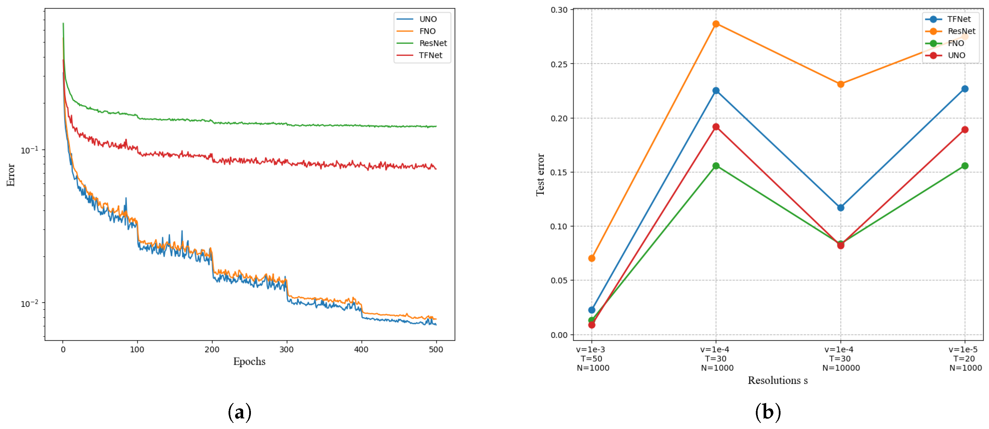
| UNO | 414,517 | 38.99s | 0.0128 | 0.1879 | 0.0834 | 0.1856 |
| FNO | 6,558,53 | 45.80s | 0.0135 | 0.1551 | 0.0835 | 0.1524 |
| ResNet | 266,641 | 78.47s | 0.1716 | 0.2871 | 0.2311 | 0.2753 |
| TF-Net | 7,451,724 | 47.21s | 0.0225 | 0.2253 | 0.1168 | 0.2268 |
From Figure 8, FNO and UNO are found to have better results. By comparing time and data points,suitable algorithms are selected. The error of UNO and FNO algorithm can continue to decrease steadily with the number of iterations, which has great advantages compared with other models. The error of UNO algorithm drops faster, with an obvious decrease process at 100, 200, 300 and 400, showing a continuous jitter decreasing trend, and has obvious advantages in solving the equation. The RENET and TFNET models are less effective, and compared with UNO and FNO, the curves are relatively smooth and the errors are larger during the iteration. Figure 8 also compares the experimental error of UNO and FNO, RENET, and TFNET on the dataset. The figure shows the data points N=10000 and T=50. When the viscosity coefficient is , the UNO error is the smallest, and UNO has higher accuracy. When the data point N=1000, UNO is worse than FNO, but when the data pont increases, N=10000, the UNO error is always the smallest compared with other algorithm models.
5. Conclusions
This paper proposes an innovative method based on the combination of U-Net neural networks and Fourier neural operators, aiming to improve the accuracy and efficiency of solving partial differential equations (PDEs). By integrating the unique encoder-decoder structure and skip connections of U-Net with the deep feature processing capabilities of Fourier transforms in the frequency domain, the method fully leverages the strengths of U-Net in spatial feature extraction and the capabilities of Fourier transforms in frequency-domain feature processing. This combination not only preserves spatial details but also captures both high-frequency and low-frequency characteristics of PDE solutions through frequency-domain analysis, thereby significantly enhancing solving accuracy. Experimental results demonstrate that, compared to traditional methods, this approach performs exceptionally well in various complex PDE-solving tasks, achieving higher accuracy. While the method reduces reliance on large-scale datasets, high-quality datasets remain crucial for training the model when dealing with complex physical systems. Future research could explore ways to further improve the model’s generalization ability in data-scarce scenarios.
Author Contributions
- TZ: Conceptualized and designed the research plan, took the lead in the collection and preliminary analysis of experimental data. Additionally, TZ polished the language and proofread the format of the entire paper, ensuring its professionalism in expression and presentation. - XRZ: Conducted in - depth statistical analysis of the data, provided key insights into the interpretation of the results, and participated in writing the core content of the discussion section, making significant contributions to the discussion and interpretation of the research findings
Funding
This research received no external funding.
Institutional Review Board Statement
Not applicable.
Informed Consent Statement
Not applicable.
Conflicts of Interest
The authors declare no conflicts of interest.
References
- Machine learning and computational mathematics. arXiv 2020, arXiv:2009.14596, 2020.
- Han, Jiequn, and Arnulf Jentzen, Deep learning-based numerical methods for high-dimensional parabolic par- tial differential equations and backward stochastic differential equations, Communications in mathematics and statistics. 5.4 (2017): 349-380. [CrossRef]
- Weinan. E, Jiequn Han, and Arnulf Jentzen, Algorithms for solving high dimensional PDEs: from nonlinear Monte Carlo to machine learning, Nonlinearity. 35.1 (2021): 278. [CrossRef]
- Weinan E and Bing Yu, The deep Ritz method: A deep learning-based numerical algorithm for solving variational problems, Communications in Mathematics and Statistics. 6(1):1?12, 2018. [CrossRef]
- Turner, M. Jon, et al, Stiffness and deflection analysis of complex structures, Journal of the Aeronautical Sci- ences. 23.9 (1956): 805-823. [CrossRef]
- Richtmyer, Robert D., and Keith W. Morton, Difference methods for initial-value problems, Malabar. (1994). [CrossRef]
- Jameson, Antony, Wolfgang Schmidt, and Eli Turkel, Numerical solution of the Euler equations by finite volume methods using Runge Kutta time stepping schemes, 14th Fluid and Plasma Dynamics Conference. (1981).
- Dockhorn, T. A discussion on solving partial differential equations using neural networks. arXiv 2019, arXiv:1904.07200, 2019. [Google Scholar]
- Hornik K., Stinchcombe M., White H. Universal approximation of an unknown mapping and its derivatives using multilayer feedforward networks[J]. Neural Networks, 1990, 3(5): 551-560. [CrossRef]
- Lagaris I., Likas A., Fotiadis D. Artificial neural networks for solving ordinary and partial dif ferential equations[J]. IEEE Transactions on Neural Networks, 1998, 9(5): 987-1000. [CrossRef]
- Lagaris I., Likas A., Fotiadis D. Artificial neural networks for solving ordinary and partial dif ferential equations[J]. IEEE Transactions on Neural Networks, 1998, 9(5): 987-1000. [CrossRef]
- Winovich N., Ramani K., Lin G. Convpde-uq: Convolutional neural networks with quantified uncertainty for heterogeneous elliptic partial differential equations on varied domains[J]. Journal of Computational Physics, 2019, 394: 263-279. [CrossRef]
- Long Z.C., Lu Y.P., Ma X.Z., Dong B. Proceedings of machine learning research: volume 80 PDE-net: Learning PDEs from data[M]. PMLR, 2018: 3208-3216.
- Long Z.C., Lu Y.P., Dong B. Pde-net 2.0: Learning pdes from data with a numeric-symbolic hybrid deep network[J]. Journal of Computational Physics, 2019, 399: 108925. [CrossRef]
- LeCun Y, Bottou L, Bengio Y, et al. Gradient-based learning applied to document recognition[J]. Proceedings of the IEEE, 1998, 86(11): 2278-2324. [CrossRef]
- Fan, Yuwei, et al, A multiscale neural network based on hierarchical matrices, Multiscale Modeling Simula- tion. 17.4 (2019): 1189-1213. [CrossRef]
- Hornik K, Stinchcombe M, White H. Multilayer feedforward networks are universal approximators[J]. Neural networks, 1989, 2(5): 359-366. [CrossRef]
- Mathieu, M.; Henaff, M.; LeCun, Y. Fast training of convolutional networks through ffts. arXiv 2013, arXiv:1312.5851, 2013. [Google Scholar]
- Vahid K A, Prabhu A, Farhadi A, et al. Butterfly transform: An efficient fft based neural architecture design[C]//2020 IEEE/CVF Conference on Computer Vision and Pattern Recognition (CVPR). IEEE, 2020: 12021-12030.
- Kovachki, Nikola, et al, Neural operator: Learning maps between function spaces,arXiv preprint. arXiv:2108.08481 (2021). [CrossRef]
- Li, Zongyi, et al, Fourier neural operator for parametric partial differential equations,arXiv preprint. arXiv:2010.08895 (2020). [CrossRef]
- Kushnure D T and Talbar S N.Ms-Unet: A Multi-Scale Unet with Feature Recalibration Approach for Automatic Liver and Tumor Segmentation in Ct Images[J].Computerized Medical Imaging and Graphics,2021,89:101885. [CrossRef]
- Isensee F, Kickingereder P, Wick W,et al.Brain Tumor Segmentation and Radiomics Survival Prediction: Contribution to the Brats 2017 Challenge[C]//Brainlesion: Glioma, Multiple Sclerosis, Stroke and Traumatic Brain Injuries: Third International Workshop, BrainLes 2017, Held in Conjunction with MICCAI 2017, Quebec City, QC, Canada, September 14, 2017, Revised Selected Papers 3, 2018.Springer,287-297.
Figure 2.
(a) 100 solutions visulization.(b) 1000 solutions visulization. (c) 2000 solutions visulization. (d) 8000 solutions visulization.
Figure 2.
(a) 100 solutions visulization.(b) 1000 solutions visulization. (c) 2000 solutions visulization. (d) 8000 solutions visulization.
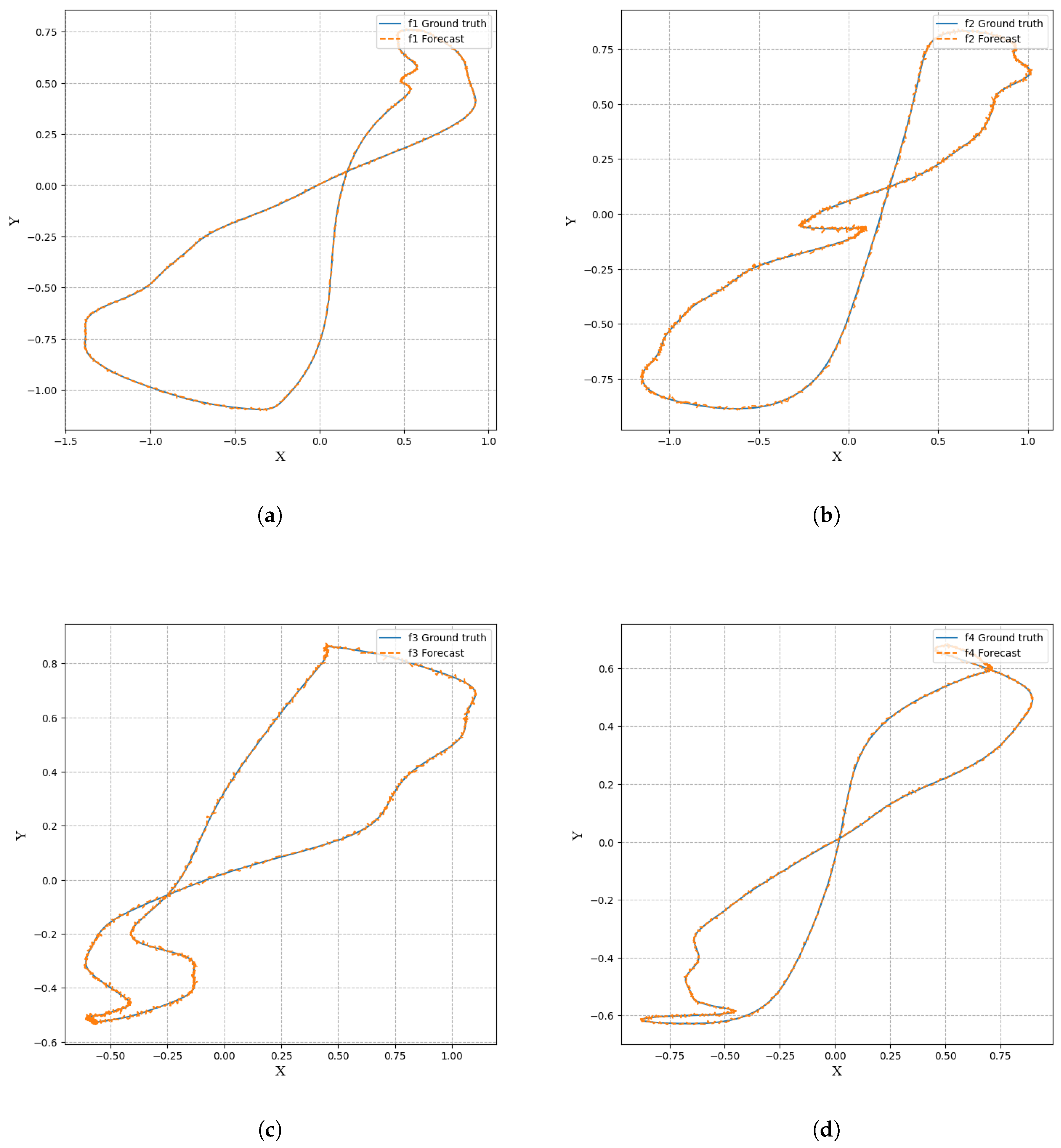
Figure 3.
(a) Epochs(b) Algorithm contrast.
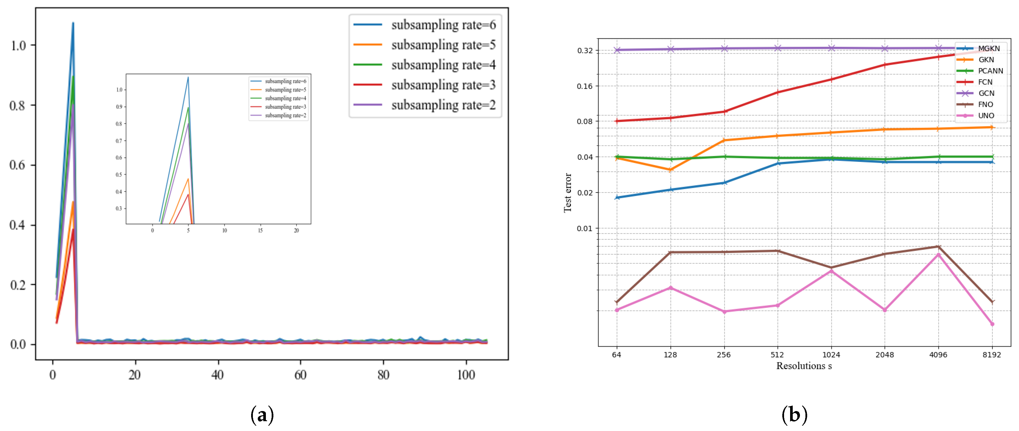
Figure 4.
Visualization error map
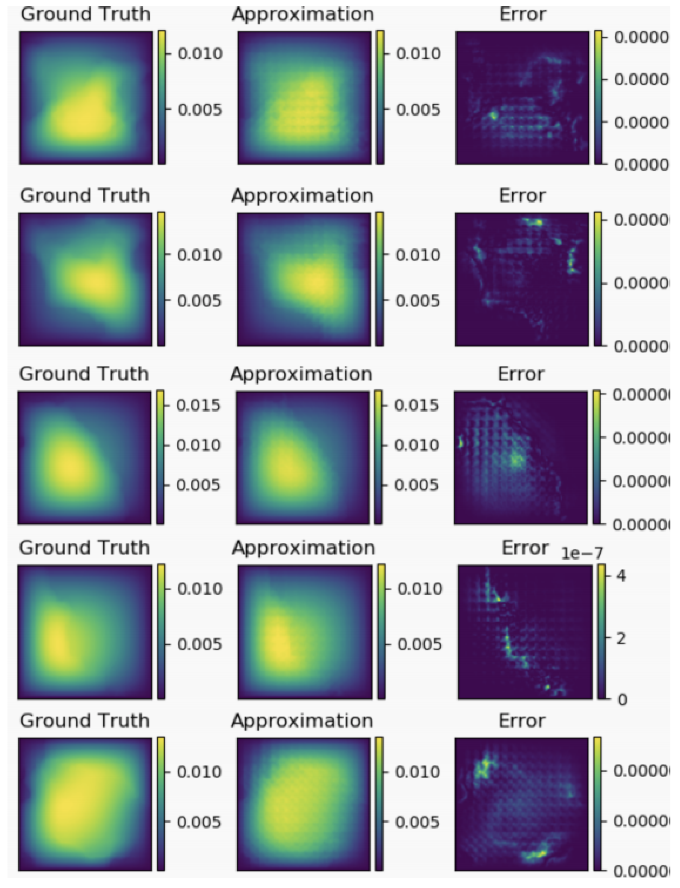
Figure 5.
(a) Fourier layer number analysis Fig.(b) Visualization error map.
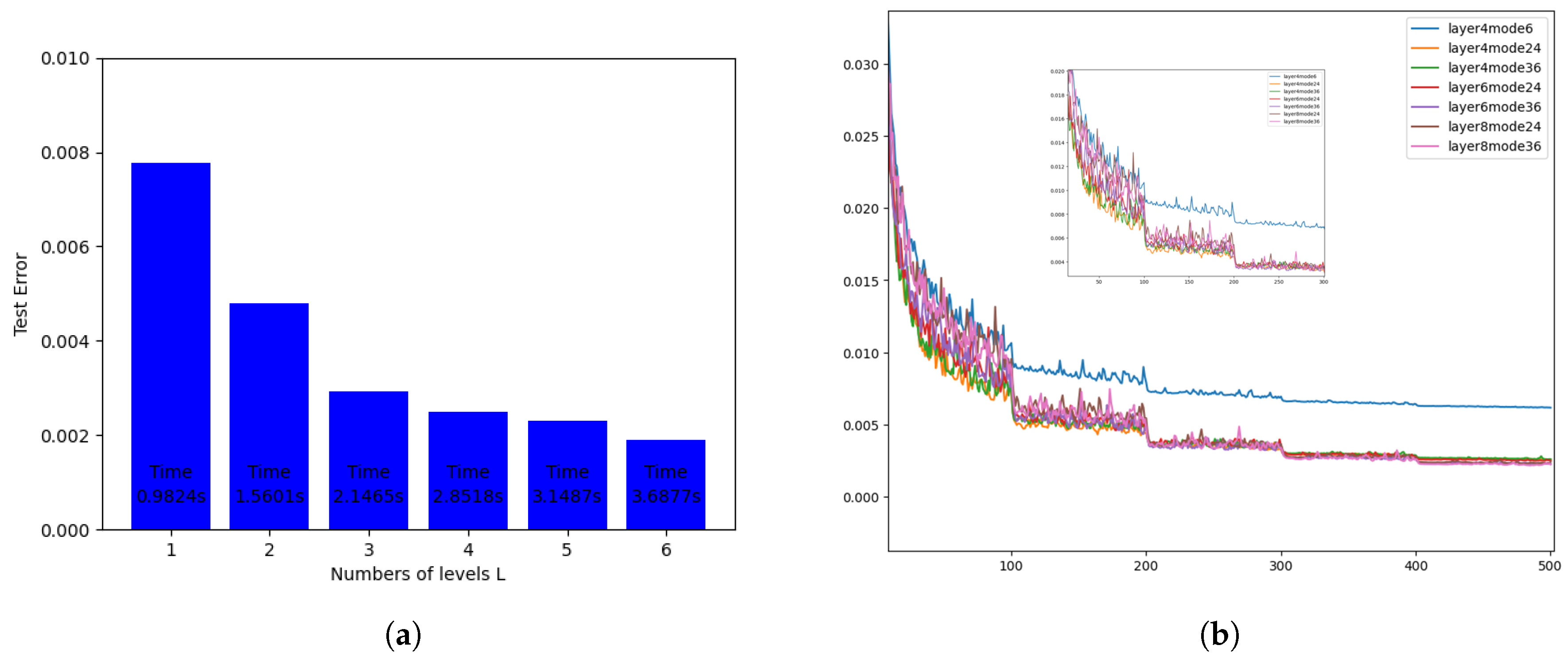
Figure 6.
The training error plots for each model.
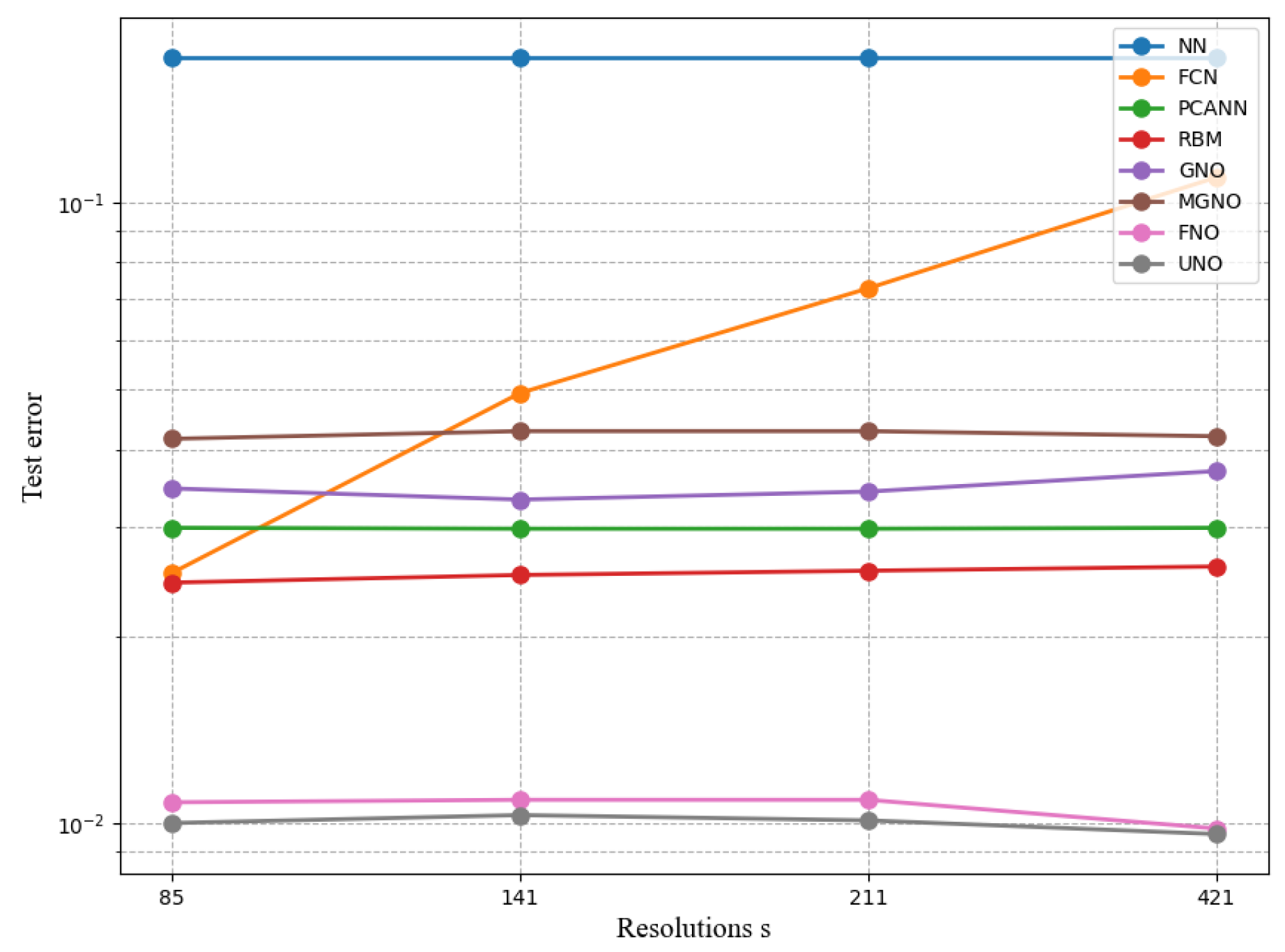
Figure 7.
Visualization error map
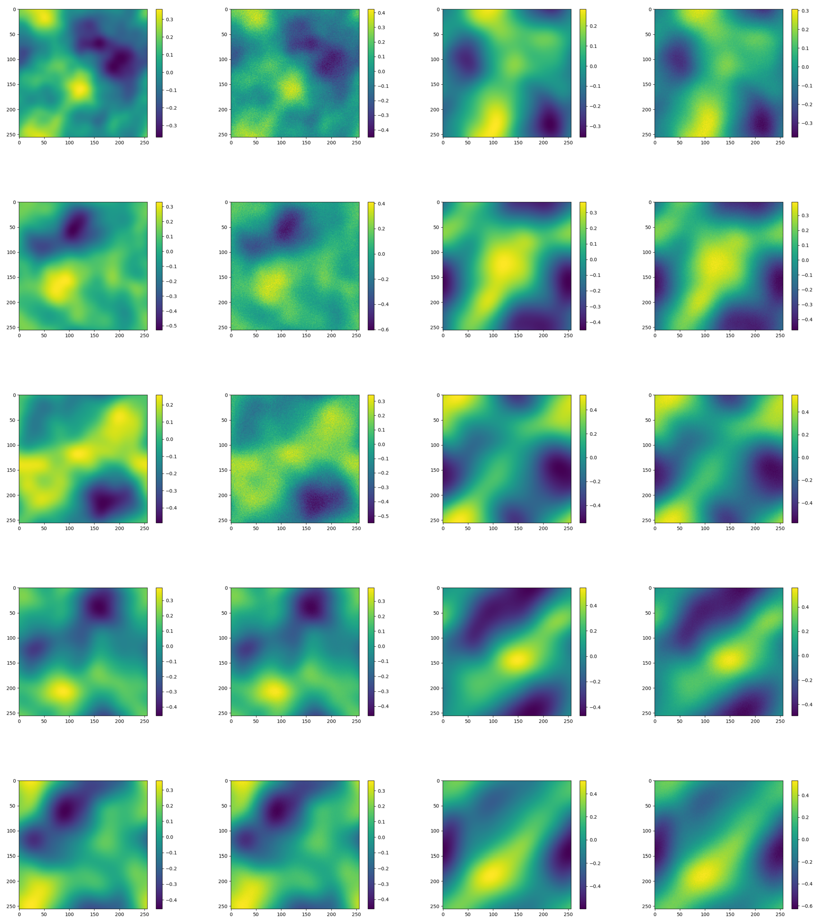
Figure 8.
(a) Epochs.(b)Resolutions.
Disclaimer/Publisher’s Note: The statements, opinions and data contained in all publications are solely those of the individual author(s) and contributor(s) and not of MDPI and/or the editor(s). MDPI and/or the editor(s) disclaim responsibility for any injury to people or property resulting from any ideas, methods, instructions or products referred to in the content. |
© 2025 by the authors. Licensee MDPI, Basel, Switzerland. This article is an open access article distributed under the terms and conditions of the Creative Commons Attribution (CC BY) license (http://creativecommons.org/licenses/by/4.0/).
Copyright: This open access article is published under a Creative Commons CC BY 4.0 license, which permit the free download, distribution, and reuse, provided that the author and preprint are cited in any reuse.


