
Submitted:
06 November 2023
Posted:
06 November 2023
You are already at the latest version
Abstract
Partial differential equations (PDEs) are used to describe a wide range of phenomena, such
as heat transfer, fluid dynamics, and quantum mechanics. By solving PDEs, we can ob-
tain insights into the behavior of the system and make predictions about its future evolution.
Conventional numerical methods for obtaining the approximate solutions of PDEs may re-
quire extensive computational resources and time, especially for complex PDEs and large-
scale problems. The recently developed physics-informed neural network (PINN) has shown
promise in a variety of scientific and engineering fields by incorporating physical laws into the
loss functions of the neural network (NN). In addition, the training of PINN does not require
ground truth data, but it has poor generalization ability to unseen domains. On the other hand,
a convolutional neural network (CNN) has fast inference and better generalization ability, but
it requires a large amount of training data.
Taking the advantages of PINN and CNN by using Legendre multiwavelets (LMWs) as
basis functions, we introduce a new method to approach the PDEs in this paper, namely
Physics-Informed Legendre Multiwavelets CNN (PiLMWs-CNN), in order to continuously
approximate a grid-based state representation that can be handled by a CNN. PiLMWs-CNN
enable us to train our models using only physics-informed loss functions without any pre-
computed training data, simultaneously providing fast and continuous solutions that gener-
alize to previously unknown domains. In particular, the LMWs can simultaneously possess
compact support, orthogonality, symmetry, high smoothness, and high approximation order.
Compared to orthonormal polynomial (OP) bases, the approximation accuracy can be greatly
increased and computation costs can be significantly reduced by using LMWs. We applied
PiLMWs-CNN to approximate the damped wave equation, incompressible Navier-Stokes (N-
S) equation, and two-dimensional heat conduction equation. The experimental results show
that this method provides more accurate, efficient, and fast convergence with better stability
when approximating the solution of PDEs.
Keywords:
Partial differential equations
; Legendre multiwavelets
; Physics-informed neural net- work
; Convolutional neural network
1. Introduction
PDEs, as a powerful mathematical tool in classical physics, enable the comprehensive depiction, simulation, and modeling of various dynamic phenomena, including heat flow, diffusion processes, wave propagation, and the motion of fluid substances [1], owing to their inherent capability to capture the fundamental characteristics of intricate systems. However, obtaining the analytical solutions of PDEs is challenging. To address this issue, conventional numerical methods like the finite volume method (FVM) [2], finite difference method (FDM) [3], and finite element method (FEM) [4], are utilized to approximate the solutions. Despite the strength and rigor of these approaches, they may experience an exponential rise in computational complexity with grid refinement and “dimension explosion” as the independent variable’s dimension increases.
With the rapid development of deep learning (DL), which is a form of machine learning (ML) that utilizes NNs with multiple hidden layers [5], has emerged as a new paradigm in scientific computing due to its universal approximation [6] and expressive capabilities. Solving PDEs through DL has gained significant momentum. Recent researches have shown that DL holds promise in building meta-models for efficiently predicting dynamic systems. By training deep neural networks (DNNs), especially with Artificial Intelligence (AI)-based approaches, systems or even families of PDEs can be expressed, leading to exponential advancements in computing efficiency during practical usage. Unlike traditional numerical methods, DNN-based approaches can simultaneously approximate target solutions in multiple dimensions, including the time dimension. They can learn direct mappings between physical states and spatial/temporal coordinates without the need for repeated iterations at each time step [7].
Currently, an increasing number of researchers are utilizing DL methods to investigate PDEs [6,8]. Among the various studies, an important contribution that cannot be overlooked is the PINNs proposed by Raissi et al. [9]. This NN model enhances the performance of the NN model by taking into account the physical laws found in PDEs and encoding them into the NN as regularization terms. Researchers have been paying more attention to PINNs lately, and they are gradually applying them to a wider range of research fields [10]. Although PINNs can be trained with little to no ground truth data, they often fail to effectively generalize to domains that were not encountered during training [11]. However, CNN can learn the inherent laws of the data and thus have better generalization ability for new data. Furthermore, the structure and characteristics of CNN facilitate the solution of PDE. For example, CNN can simplify the solution of complex PDE by reducing the dimension, leverages powerful nonlinear approximation capabilities to handle intricate initial and boundaries conditions (ICs/BCs), and, when integrated with parallel computing and GPU acceleration, significantly improves the computational efficiency of PDE solutions. Moreover, CNN can employ multi-input methods to manage multi-variable problems, and, through end-to-end learning, it minimizes the need for manual intervention and the complexity of manual settings [9,12]. Nevertheless, CNN relies on large amounts of training data.
In this paper, we propose PiLMWs-CNN for deriving continuous solutions that can be trained with a physics-informed loss only. This method merges the benefits of i) utilizing PINNs to eliminate the necessity for extensive training data [9,13] and ii) capitalizing on the enhanced inference speed and improved generalization abilities provided by CNN [14]. The main contributions of our work are as follows:
- Construct a set of new standard orthogonal compact supported LMWs.
- Prove the compact support property of LMWs integrated twice.
- Propose a novel network called PiLMWs-CNN to obtain LMWs coefficients (LMWCs) for approximating PDEs.
The rest of the paper is organized as follows. In Section 2, we conduct a survey of related works on solving PDEs using DNNs. We analyze and discuss these works from three different perspectives: physics-informed methods, neural operators (NO) learning, and advantages and applications of combining wavelets with CNNs. In Section 3, we provide the research methods of the paper. First, we conduct a feasibility analysis on combining the Legendre wavelet bases with CNNs to solve PDEs, including the role of compactness and orthogonality. Next, we provide relevant mathematical foundations, including the construction of the LMWs. Then, we give the network architectures and pipeline used in this study. In Section 4, we apply this method to approximate the wave equation, fluid equation, and heat conduction equation, with a particular focus on the loss of physical information and the stability of the solution. In Section 5, we give the conclusions.
2. Related Work
In this section, we will discuss different approaches to solve PDEs using NNs based on various mathematical foundations.
2.1. Physics-Informed Methods
This type of methods generally involves using PDEs as the constraints on training DNNs directly [9,15]. In numerous practical applications, constraints are often imposed by generalized prior knowledge, which take the form of differential equations (DEs) and are incorporated into the model training as the components of the loss function [16]. More recently, Raissi et al. [9] introduced the concept of PINNs, which have demonstrated their potential in various scenarios [17]. There are also specialized DL libraries, like DeepXDE [16], developed specifically for solving DEs.
Treating PDEs as training constraints was initially referred to as "soft constraints" [18], as the knowledge in the form of PDEs only enforces the correctness of the predicted results without guiding the optimization process. Additionally, the modeling process takes into account additional constraints in the form of ICs/BCs. Unlike conventional numerical approaches that rely on discretizing grids [19], utilizing PDE-based constraints to train DNNs ensures continuous solutions over the entire research domain, leading to highly precise results. PINNs are particularly suitable when the underlying physics of the problem is known beforehand, as they exploit the governing laws of the physical processes during training.
These methods leverage the idea that multilayer feedforward NNs (FFNNs) can serve as universal approximators for high-dimensional functions [20]. Both DNNs and solving DEs share a common objective: to achieve accurate approximations. Whether it is the FEM using basis functions to approximate solutions within a unit or DNNs with complex structures fitting high-dimensional functions, the computed or predicted values at each unit center or sampling point should be extremely close to the actual values. The goal for DNNs is to minimize the loss function value, or residual, which should ideally approach zero. In the numerical approach, this residual represents the error in the computed solution.
However, data-driven algorithms are often the only practical choice for natural processes because the underlying physics governing them is unknown. These algorithms do not generalize beyond the distribution of training data, even though they do not ensure the preservation of the problem’s governing physics [21].
2.2. Neural Operators Learning
In response to the challenges mentioned above, the concept of NO was introduced by Lu et al. [22]. NOs are designed to learn the relationship between two infinite-dimensional function spaces. After training, these NOs can accurately predict the solution for any input function presented to them. In comparison to conventional PDE solvers, NOs offer significant computational advantages. These NOs are based on the concept of universal operator approximation, as proposed by Chen et al. [23], which is similar to the theory of universal function approximation. Kovachki et al. [24] have conducted rigorous mathematical analysis and provided theoretical guarantees for the effectiveness of NOs.
By employing this methodology, DL can successfully obtain mesh-free, infinite-dimensional linear and nonlinear operators. Chen et al. [23] developed an initial prototype of NO methods based on operator theory, drawing inspiration from linear algebra and functional analysis. Currently, there are three popular instances in this area, which are Deep Operator Network (DeepONet) [25], Graph Neural Operator (GNO) [26], and Fourier Neural Operator (FNO) [27]. The DeepONet architecture comprises of two NNs: the branch NN and the trunk NN. The branch NN handles the input function, while the trunk NN is responsible for generating the output function at a specific sensor point. In DeepONet, the output is derived by taking the inner product of these NNs. The GNO focuses on learning mappings in infinite-dimensional spaces by combining nonlinear activation functions with a specific category of integral operators. Nevertheless, GNO may become unstable as the number of hidden layers increases. These advanced networks possess exceptional feature representation capabilities, and when combined with the idea of approximating functionals using the prototype network, the NOs become infused with boundless vitality. The FNO is an innovative approach inspired by the well-known Fourier transform (FT). Building upon the GNO, the FNO was introduced as an enhanced method to learn network parameters in Fourier space [27]. The FNO employs the fast FT (FFT) to perform spectral decomposition on the input signal, subsequent to calculating the convolution integral kernel in the Fourier domain. One notable limitation of FNO stems from the frequency localization of basis functions in FFTs, which hinders its ability to provide spatial resolution [28]. Consequently, FNO’s performance may be adversely affected when dealing with complex BCs.
An alternative method to tackle this issue is to employ wavelets, which exhibit both spatial and frequency localization properties [28]. By incorporating spatial information, wavelets demonstrate enhanced ability in handling signals with discontinuities and spikes, thus surpassing the pattern learning capabilities of FFTs when specifically dealing with image data. Wavelets have found applications in various domains, such as compression of fingerprints, iris recognition, denoising of signals, analysis of motion, and detection of faults, among other areas. The literature also highlights the utilization of wavelets in NNs [29]. In their work, Gupta et al. [30] proposed an operator that utilizes MW decomposition (MWD). This approach involves the use of four distinct NNs to calculate wavelet kernels. Specifically, the network architecture includes a fully connected NN (FNN), a CNN, and a Fourier integral layer similar to FNO. As the FNN represents the coarse scale, the combination of the latter three networks computes the detailed wavelet coefficients. As a result, MWD can be considered an improvement over FNO. Given that the solution of a PDE is obtained by calculating the inverse operator map between the input and the solution space, Gupta et al. aim to transform the problem of learning PDEs into a domain where a more compact representation of the operator can be obtained. In order to achieve this, they proposed an approach for learning the operator, based on MWs, which allows for compression of the associated kernel. By explicitly incorporating the inverse MW filters, they learn the projection of the kernel onto fixed MW polynomial bases. The use of MWs offers a natural basis for the MW subspace, using OPs with respect to a specific measure, and employing suitable scale/shifts to capture locality at different resolutions. Tripura et al. [31] introduced a NO, termed Wavelet Neural Operator (WNO), which utilizes spectral decomposition to learn mappings between infinite-dimensional function spaces. The proposed WNO demonstrates its effectiveness in dealing with highly nonlinear families of PDEs that involve discontinuities and abrupt changes in both the solution domain and boundary.
2.3. Wavelets and CNN
It is essential to highlight that the wavelet transform (WT) is a signal processing technique that exhibits the properties of localization in both the time and frequency domain. This attribute makes it a powerful tool for analyzing local features [32]. Consequently, Li et al. [33] developed a deep wavelet NN (DWNN) based on the PINNs approach. The employment of wavelets enables the extraction of multi-scale and detailed features, resulting in enhanced performance in solving PDEs.
However, it is well known that wavelet functions are not simultaneously symmetric, orthogonal, and compact supported. These challenges are overcome by LMWs, also referred to as more general, vector-valued polynomial types of wavelets [34], which simultaneously have all three of these properties. This leads to high smoothness and high approximation order and suggests that LMWs can outperform scalar wavelets in a variety of applications [35].
Therefore, some researchers have focused on investigating how to solve PDEs using the Legendre wavelets method. It is worth mentioning that Legendre wavelets have both spectral accuracy and orthogonality, as well as other properties mentioned about wavelets [36]. For example, the wavelet technique can transform complex problems into a system of algebraic equations. Heydari et al. [37] presented a numerical technique utilizing two-dimensional Legendre wavelets to solve fractional PDEs with Dirichlet BCs. The method involved using operational matrices for fractional integration and derivatives to obtain numerical solutions to the problems under consideration. The approach presented by Abbas et al. [38] primarily focuses on converting the fundamental DEs into integral equations through integration. This is accomplished by approximate representation of the diverse signals embedded in the equations using truncated orthogonal series . Subsequently, the operation matrix of integration, denoted as P, is employed to remove the integral operations.
Meanwhile, we found in the research that there are many applications for the combination of wavelets and CNN. It was discovered that a CNN can be considered a simplified version of multiresolution analysis (MRA). This revelation highlights the fact that conventional CNNs fail to capture a substantial portion of the spectral information accessible through MRA. Therefore, Fujieda et al. [39] introduced the idea of wavelet CNNs, which combine MRA and CNNs within a single model. This strategy enables the exploitation of spectral information that is frequently neglected in conventional CNNs but is essential in various image processing tasks. Zhao et al. [40] suggested a Wavelet-Attention CNN (WA-CNN) for image classification purposes. They explored Discrete WT (DWT) in the frequency domain and devised a novel WA block, which solely implements attention in the high-frequency domain. DWT exhibits superior down-sampling information quality in the image processing domain, thereby significantly minimizing the loss of down-sampling information in CNN. Guo et al. [41] developed a method for intelligent fault diagnosis of rolling bearings, utilizing WT and deformable CNN. Their research highlights the significance of selecting appropriate wavelet bases in the WT. Different wavelet bases have a substantial influence on the resulting time-frequency map. In the context of CNNs, WT is developed and employed for breast cancer detection [42]. The adaptive wavelet pooling layers, as proposed by the Wolter et al. [43], make use of fast WT (FWT) to lower the feature resolution. Through FWT, the input features are decomposed into various scales, resulting in a reduction of feature dimensions by eliminating the fine-scale subbands. This approach introduces additional flexibility by optimizing the wavelet basis functions and weighting coefficients at different scales, thus avoiding high repetition.
The findings above indicate that CNNs exhibit strong performance when handling multidimensional data, such as images and speech signals. In fact, these networks have been employed in a PINN, primarily within the domain of image processing. Inspired by the above researches, we consider combining LMWs with CNN to approach PDEs, and conduct experiments on three different types of equations to validate the effectiveness and accuracy of this approach.
3. Method
3.1. Feasibility Analysis
By integrating LMWs with CNN for solving PDEs, this approach capitalizes on four key advantages, thereby enhancing the modeling and analysis capabilities in PDE solving and delivering more precise predictions and solutions.
- Multiscale Representation: PDEs often involve spatial features at different scales. By using the LMWs, it provides the capability of multiscale representation, which can better capture the features of the input data at different scales. This is crucial for analyzing and solving PDEs involving multiscale spatial features.
- Local Correlation Modeling: The mathematical models in PDEs often assume that the system’s behavior is influenced by its local neighborhood. The LMWs have good properties in capturing the local correlation of input data effectively. By using convolution operations in CNN, it can leverage this local correlation and perform local feature extraction on the input data, which helps in describing the local behavior in PDEs more accurately. Bedford et al. [44] prove rigorously that good approximation "locally" guarantees good approximation globally.
- Translation Invariance: Analysis of spatial translation invariance is often required for input data in PDEs. The translation invariance property of LMWs ensures that the translation of input signals does not affect the representation of their MW coefficients (MWCs). In CNN, convolution operations can preserve the translation invariance of input data, better meeting the requirement of translation invariance in PDEs.
- Explanation and Interpretability: LMWs have good explanatory and interpretable properties, providing insights into the features and structure of PDEs. By combining LMWs with CNN, we can leverage the explanatory power of MWs and the learning capability of CNN to better understand and interpret the feature representations of PDEs. In fact, Restricted Boltzmann machines (RBMs) [45] and other variants of DL models, such as deep belief networks and autoencoders, have a clear advantage in providing explanations and interpretability.
Furthermore, the compact support property of LMWs offers several advantages [46,47] when applied to solving PDEs with NNs.
- Reduced computational cost: The compact support of LMWs enables a smaller set of wavelet coefficients to be considered, thereby reducing the computational burden associated with representing the solution as a wavelet series.
- Localized feature extraction: LMWs are well-suited for extracting localized features within the solution, facilitating the NN’s ability to comprehend the underlying structure of the PDE.
- Regularization effect: LMWs’ compact support property inherently creates a regularization effect in the NN, which reduces overfitting and improves generalization performance.
- Adaptability to different scales: LMWs readily adapt to various scales by adjusting the wavelet coefficients, permitting the NN to capture features at different resolutions.
- Robustness to noise: LMWs’ compact support enhances their resilience to noise and other imperfections in the input data, enabling more accurate solutions to be obtained when employed in conjunction with NNs.
Based on the aforementioned analysis, a strong correlation between LMWs, CNNs, and PDEs becomes apparent. Notably, the compact support property of LMWs offers numerous advantages when resolving PDEs via NNs. These distinctive features render the integration of wavelets and CNNs particularly appealing for PDE solutions, providing the authors with a promising avenue to approximate PDEs. Consequently, it piques the authors’ curiosity and motivates further exploration and in-depth experimentation with this approach.
3.2. Foundations of Multiwavelet Bases Construction in Mathematics
Families of functions ,
obtained from a single function by dilation and translation and serve as the basis for , are known as wavelets [48].
In the following, we will provide an overview of the properties of the MW bases developed in [49] and introduce the necessary notations.
3.2.1. MW bases
In this subsection, we introduce a new class of wavelet-like bases referred to as MW bases, which enable sparse representations of smooth integral operators over finite intervals. Moreover, MW bases have orthogonality, compact support, vanishing moments, and other wavelet base properties. The basis functions do not overlap on a specific scale and are arranged into small groups of multiple functions (thus, MWs) sharing the same support. One notable benefit of this construction is its simplicity.
One-dimensional construction
Our focus will initially be limited to , and we now proceed to establish a basis for . Each basis consists of dilates and translates of a finite set of functions . Specifically, these bases consist of orthonormal systems
where the functions are piecewise polynomials, they become zero outside the range of , and possess vanishing moments, making them orthogonal to low-order polynomials,
Besides, we implement the MRA approach, and suppose , for , we define a space of piecewise polynomial functions,
It is clear that the space has a dimension of and
For , we define the -dimensional space (the MW subspace) to be the orthogonal complement of in ,
therefore, we can inductively derive the decomposition
Suppose that functions form an orthogonal basis for , that is . More generally,
Since is orthogonal to , the first n moments of vanish,
The -dimensional space is spanned by orthogonal functions , of which n are supported on the interval and n on . Generally, the space is spanned by functions obtained from by translation and dilation. There is some freedom in choosing the functions , subject to the restriction of orthogonality, we can uniquely determine them by imposing normality and further vanishing moments, except for sign.
Completeness of one-dimensional construction
We define the space
and observe that . Here the closure is defined with respect to the -norm, , where the inner product .
Let be an orthonormal basis for , in accordance with -, the set forms a complete orthonormal basis for . We refer to as the MW bases of order n for .
3.2.2. Multiple-dimensional construction
For any positive integer d, the bases construction for can be extended to some other function spaces as well, such as . The basis for , which serves as an example of the construction for any finite-dimensional space, is now given in order to outline this extension. We establish the space
where is defined by . Furthermore, we define to be the orthogonal complement of in ,
is then the space generated by the orthonormal basis
For each basis element of these elements, it has no projection on any low-order polynomial,
Dilations and translations of the span the space ; low-order polynomials
are also included in the basis of , which is made up of these functions.
3.3. Construct LMWs
In this part, our primary focus is the development of MW bases based on Legendre polynomials, which we refer to as LMWs. We present detailed construction procedures and provide the necessary proofs to support our approach.
3.3.1. Legendre polynomials
Legendre polynomials are polynomials defined on the and have a recursive formula [50]:
In order to be consistent with the previous knowledge, we consider a transformation to fix the discussion interval at and construct the standard orthogonal basis of . Finally, a similar transformation can be performed to return to the desired interval. The implementation details can be found in literature [51]. Therefore, according to , Legendre polynomials on can be expressed as follows through translation and expansion transformations:
Further, is an orthonormal basis in .
3.3.2. LMWs
Now, we use Legendre polynomials as LMW multiscaling function [52], to construct the Legendre mother multiwavelet [53] as
By the properties of vanishing moments and standard orthonormality, can be uniquely determined. Figure 1 shows the plots of these four Legendre mother multiwavelets.
Then, we construct the LMWs by translating and dilating the mother multiwavelet and they can be expressed as
In addition, is compact supported on the interval , and forms a complete orthonormal basis for .
3.3.3. Compact support
Given the common use of second-order PDEs in physics and engineering [54], we aim to solve them in the [55] by integrating twice. Then, we denote
Lemma 1.
Theorem 1.
is compact supported on .
Proof. For , if , if ,
Let then . So, the transformation of (3.20) is as follows,
The theorem holds true.
3.3.4. Function approximation
We employ the tensor product of multiple one-dimensional () basis functions to derive basis functions in multiple dimensions [56], building upon equation discussed earlier. To simplify the expression, we still use as a basis function in , so that we have the following equation:
With discrete MWCs on a grid , we obtain a continuous LMW as follows:
Our goal is to find MWCs such that as nearly as possible resembles the PDE solution. By taking the corresponding derivatives of the LMWs, one can directly obtain the partial derivatives of with respect to .
3.4. Neural Network Architecture
Figure 2 showcases the network architectures employed for the incompressible N-S equation and the damped wave equation. The domain’s occupancy grid at a timepoint t is represented by and contains Dirichlet BCs. We utilize a U-Net architecture [11] internally for the N-S equation, the damped wave equation, however, only required a basic 3-layer CNN. These networks were employed to calculate residuals ,which are then added to to derive the MWCs of the next time-step . Thus, we mean-normalize the coefficients to zero, that is .
Pipeline
As depicted in Figure 3, PiLMWs-CNN employs a CNN (PDE Model) to map discrete LMWCs and BCs from a timepoint to LMWCs at a subsequent timepoint . By iteratively applying the PDE Model on the LMWCs, the simulation can be propagated in time. Efficient computation of continuous LMWs is achievable using transposed convolutions (refer to (3.23)) with LMWs, as illustrated in Figure 4.
Training procedure
As demonstrated in Figure 5, our method adopts a training process similar to that in reference [11]. Initially, we create a randomized training pool consisting of domains and LMWCs. Since all LMWCs can be set to zero at first, ground truth data is not required. The PDE model then uses the random minibatch (batch size = 50) that we extracted from the training pool to predict the LMWCs for the next time step. Next, with the goal of optimizing the PDE model weights via gradient descent, we compute a physics-informed loss inside the volume spanned by the LMWCs of the minibatch and the predicted LMWCs. We employ the Adam optimizer (learning rate = ) for this purpose. We update the training dataset with the newly predicted LMWCs during the training process to gradually replenish the pool with more realistic training data. From time to time, we reset all of the LMWCs in the training pool to zero, which enables us to learn the warm-up phase from the ground up.
Physics-informed loss
Drawing parallels with reference [11], the PiLMWs-CNN approach integrates the benefits of both physics-constrained methodologies [48] and physics-informed strategies [9]. This method shows the ability to generalize to new domain geometries and yields continuous solutions that avoid the drawbacks of a discretized loss function based on finite differences by using a CNN to manage LMWCs, which can be thought of as a discrete hidden latent representation for a continuous implicit field description based on LMWs. We aim to minimize the integrals of the squared residuals of the PDEs over the domain / domain boundaries and time steps by optimizing the LMWCs. We uniformly randomly choose points inside the designated integration domains in order to compute these integrals. Within the domain, we require two loss terms for the damped wave equation 26:
The boundary loss term is:
For the integral to be computed, it is imperative that the residuals have bounded variation.
4. Results
In this section, we applied PiLMWs-CNN to approximate the damped wave equation, the incompressible N-S equation, and the two-dimensional heat conduction equation. Through quantitative evaluation and stability analysis, it is evident that our method achieves higher accuracy and provides better approximation for both the governing equations and BCs. The figures below are displayed in TensorFlow after training.
Example 1. The Damped Wave Equation appears as a mathematical model in biology and physics [57]. It is important in geophysics, general relativity, quantum mechanics, and plasma physics. We consider the following equation with constant positive damping:
Here, k is the stiffness constant, is a damping constant. Wave equation solutions are essential for understanding the concepts in fluid dynamics, optics, gravitational physics and electromagnetism. Moreover, for large damping constants , converges towards the Laplace equation solution [11].
Table 1 compares the losses of our method with that of reference [11]. We trained with LMWs (Figure 4) in the spatial dimensions, and observed a much better performance. From the result of , it can be seen that our method follows the physical laws well.
As shown in Figure 6, our method produces stable results for the damped wave equation.
Example 2. The Incompressible N-S equations are a set of PDEs that describe the movement of viscous fluids. These equations are derived by applying Newton’s second law of motion to an incompressible Newtonian fluid. The resulting equation is known as the N-S equation written in vector notation:
The equations take into account factors such as the dynamic viscosity , pressure p , fluid velocity vector , and the fluid’s density . They can be used to model a wide range of phenomena, like the flow of water in a pipe, blood in an artery, and air over an airplane wing, weather patterns in the atmosphere, and even the flow of stars in a galaxy. In our tests, we don’t take into account the external factors . For given initial conditions , and BCs, these pair of equations need to be resolved. We are taking into account the Dirichlet BC, where the velocity field is set to at the boundaries of the domain
We conducted an extensive study on the stability of PiLMWs-CNN when applied to the incompressible N-S equations. The investigation involved hundreds of iterations on the DFG benchmark [58] problem at Re = 100 (Re represents the Reynolds number). Figure 7 shows the curves of and , where is a momentum loss term defined as
The results clearly demonstrate the superiority of our approach in terms of both accuracy and stability. This significant improvement highlights the effectiveness of our method over the existing reference [11]. Furthermore, following the same approach as implicit PINNs and Spline nets, which involves computing losses based on physics-informed losses, PiLMWs-CNN calculated and and achieved lower loss values, as shown in Table 2. This demonstrates the enhanced effectiveness of our method in approximating the solutions of PDEs.
Since the proposed method in this paper utilizes physics-informed loss computation during model training, which is primarily based on the residual concept, it aligns with the idea of -best approximate solution [51] or -approximate approach [59] that have been proposed in recent years for numerical solutions of PDEs and fractional DEs (FDEs). Therefore, as a final example, we intend to apply the PiLMWs-CNN method to the two-dimensional heat conduction equation to observe its approximation performance.
Example 3. The Two-dimensional heat conduction equation is a PDE that governs the thermal conduction and heat transfer within a medium. Mathematically, it is defined as:
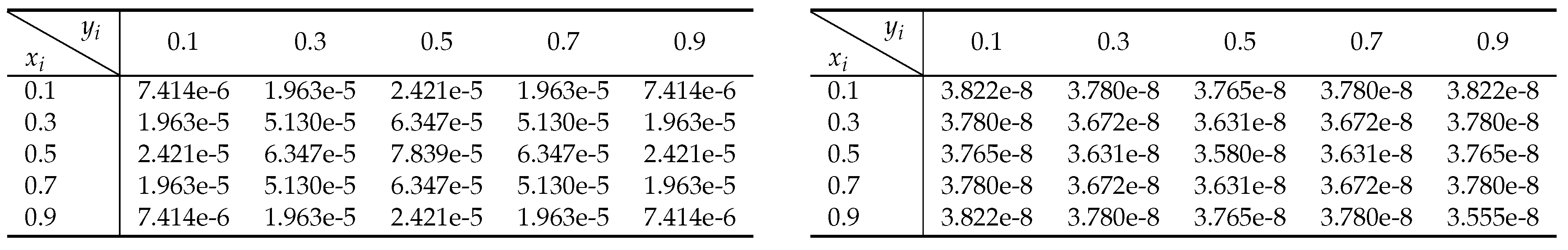
The exact solution of is We conducted the experiment for Ex.3 using the same network structure as the damped wave equation. represents the boundary loss, calculated in a manner similar to equation , while signifies the equation loss, calculated similarly to equation . From Table 3, it can be observed that the absolute errors computed by our method(right) are smaller. Figure 8 demonstrates a progressive reduction in the boundary loss of the heat conduction equation (reaching ) as the iterations progress, while the equation’s loss stabilizes (reaching ). This indicates that our method is capable of more accurately capturing the physical laws of the equation.

Table 3.
The absolute errors for Ex.3(). The left subtable is computed by Shifted-Legendre orthonormal method [51], and the right is computed by PiLMWs-CNN(ours).
Table 3.
The absolute errors for Ex.3(). The left subtable is computed by Shifted-Legendre orthonormal method [51], and the right is computed by PiLMWs-CNN(ours).
 |
5. Conclusions
This paper presents an approach to approximate PDEs by training a continuous PiLMWs-CNN utilizing solely physics-informed loss functions. A feasibility analysis of this method was conducted, properties of LMWs were analyzed, and their advantages in solving PDEs were discussed. Furthermore, the construction theory and methods of LMWs were also provided. The PiLMWs-CNN utilizes the ability of CNN in fast modeling complex systems in solving PDEs to process LMWCs through CNN, trains the network using physics-informed loss function. The experimental results show that this method is more effective, more accurate, and yields more stable solutions.
In the future, we will conduct further research on the application of the algorithm proposed in this paper for solving FDEs. This research will encompass the exploration of solution methods and network structures for constant-order, variable-order, and fractional PDEs. In addition to accuracy and stability measures, we will also investigate and experiment with other evaluation metrics. For instance, in the context of the previously mentioned damping wave equation, we will examine the doppler effect, wave reflections, as well as the drag and lift coefficients at different Reynolds numbers in the N-S equation. This assessment from a physical application perspective will provide a deeper evaluation of the algorithm’s performance and facilitate a gradual optimization of both the algorithm and the network.
Furthermore, a multigrid LMWs CNN might be contemplated for the further refinement of solutions at the boundary layers. Our method’s fully differentiable feature might also be useful in situations involving gradient-oriented shape optimization, optimal control, reinforcement learning, and sensitivity analysis. We firmly believe that the performance of upcoming ML-based PDE solvers with generalization capabilities will be positively impacted by the shift from explicit physics-constrained losses to implicit physics-informed losses on continuous fields, supported by discrete latent descriptions like LMWCs.
Acknowledgments
This work was supported by the Science and Technology Development Fund (FDCT) of Macau under Grant No. 0071/2022/A.
References
- Wang H, Zhao Z, Tang Y. An effective few-shot learning approach via location-dependent partial differential equation[J]. Knowledge and Information Systems, 2020, 62, 1881–1901. [CrossRef]
- Eymard R, Gallouët T, Herbin R. Finite volume methods[J]. Handbook of numerical analysis, 2000, 7, 713–1018.
- Zhang, Y. A finite difference method for fractional partial differential equation. Appl. Math. Comput. 2009, 215, 524C529. [CrossRef]
- Taylor, C.A.; Hughes, T.J.; Zarins, C.K. Finite element modeling of blood flow in arteries. Comput. Methods Appl. Mech. Eng. 1998, 158, 155C196. [CrossRef]
- LeCun Y, Bengio Y, Hinton G. Deep learning[J]. nature, 2015, 521, 436–444. [CrossRef]
- Wu K, Xiu D. Data-driven deep learning of partial differential equations in modal space[J]. Journal of Computational Physics, 2020, 408, 109307. [CrossRef]
- Huang S, Feng W, Tang C, et al. Partial Differential Equations Meet Deep Neural Networks: A Survey[J]. arXiv preprint arXiv:2211.05567, 2022. [CrossRef]
- Khoo Y, Lu J, Ying L. Solving parametric PDE problems with artificial neural networks[J]. European Journal of Applied Mathematics, 2021, 32, 421–435. [CrossRef]
- Raissi M, Perdikaris P, Karniadakis G E. Physics-informed neural networks: A deep learning framework for solving forward and inverse problems involving nonlinear partial differential equations[J]. Journal of Computational physics, 2019, 378, 686–707. [CrossRef]
- Tartakovsky, A.; Marrero, C.O.; Perdikaris, P.; Tartakovsky, G.; Barajas-Solano, D. Physics-Informed Deep Neural Networks for Learning Parameters and Constitutive Relationships in Subsurface Flow Problems. Water Resour. Res. 2020, 56, e2019WR026731. [CrossRef]
- Wandel N, Weinmann M, Neidlin M, et al. Spline-pinn: Approaching pdes without data using fast, physics-informed hermite-spline cnns[C]//Proceedings of the AAAI Conference on Artificial Intelligence. 2022, 36, 8529–8538.
- Beck C, Hutzenthaler M, Jentzen A, et al. An overview on deep learning-based approximation methods for partial differential equations[J]. arXiv preprint arXiv:2012.12348, 2020. [CrossRef]
- Jin X, Cai S, Li H, et al. NSFnets (Navier-Stokes flow nets): Physics-informed neural networks for the incompressible Navier-Stokes equations[J]. Journal of Computational Physics, 2021, 426, 109951. [CrossRef]
- Wandel N, Weinmann M, Klein R. Teaching the incompressible Navier-CStokes equations to fast neural surrogate models in three dimensions[J]. Physics of Fluids, 2021, 33(4). [CrossRef]
- Lagaris I E, Likas A, Fotiadis D I. Artificial neural networks for solving ordinary and partial differential equations[J]. IEEE transactions on neural networks, 1998, 9, 987–1000. [CrossRef]
- Lu L, Meng X, Mao Z, et al. DeepXDE: A deep learning library for solving differential equations[J]. SIAM review, 2021, 63, 208–228.
- Meng X, Karniadakis G E. A composite neural network that learns from multi-fidelity data: Application to function approximation and inverse PDE problems[J]. Journal of Computational Physics, 2020, 401, 109020. [CrossRef]
- Lu L, Pestourie R, Yao W, et al. Physics-informed neural networks with hard constraints for inverse design[J]. SIAM Journal on Scientific Computing, 2021, 43, B1105-B1132. [CrossRef]
- Cuomo S, Di Cola V S, Giampaolo F, et al. Scientific machine learning through physics Cinformed neural networks: Where we are and what’s next[J]. Journal of Scientific Computing, 2022, 92, 88. [CrossRef]
- Hornik K, Stinchcombe M, White H. Multilayer feedforward networks are universal approximators[J]. Neural networks, 1989, 2, 359–366. [CrossRef]
- Lu L, Meng X, Cai S, et al. A comprehensive and fair comparison of two neural operators (with practical extensions) based on fair data[J]. Computer Methods in Applied Mechanics and Engineering, 2022, 393, 114778. [CrossRef]
- Lu L, Jin P, Karniadakis G E. Deeponet: Learning nonlinear operators for identifying differential equations based on the universal approximation theorem of operators[J]. arXiv preprint arXiv:1910.03193, 2019. [CrossRef]
- Chen T, Chen H. Universal approximation to nonlinear operators by neural networks with arbitrary activation functions and its application to dynamical systems[J]. IEEE transactions on neural networks, 1995, 6, 911–917. [CrossRef]
- Kovachki N, Lanthaler S, Mishra S. On universal approximation and error bounds for Fourier neural operators[J]. The Journal of Machine Learning Research, 2021, 22, 13237–13312.
- Lu L, Jin P, Pang G, et al. Learning nonlinear operators via DeepONet based on the universal approximation theorem of operators[J]. Nature machine intelligence, 2021, 3, 218–229. [CrossRef]
- Li Z, Kovachki N, Azizzadenesheli K, et al. Neural operator: Graph kernel network for partial differential equations[J]. arXiv preprint arXiv:2003.03485, 2020. [CrossRef]
- Li Z, Kovachki N, Azizzadenesheli K, et al. Fourier neural operator for parametric partial differential equations[J]. arXiv preprint arXiv:2010.08895, 2020. [CrossRef]
- Bachman G, Narici L, Beckenstein E. Fourier and wavelet analysis[M]. New York: Springer, 2000.
- N. Shervani-Tabar, N. Zabaras, Physics-constrained predictive molecular latent space discovery with graph scattering variational autoencoder, 2020, arXiv preprint arXiv:2009.13878. [CrossRef]
- Gupta G, Xiao X, Bogdan P. Multiwavelet-based operator learning for differential equations[J]. Advances in neural information processing systems, 2021, 34, 24048-24062.
- Tripura T, Chakraborty S. Wavelet neural operator for solving parametric partial differential equations in computational mechanics problems[J]. Computer Methods in Applied Mechanics and Engineering, 2023, 404, 115783. [CrossRef]
- Zainuddin Z, Pauline O. Modified wavelet neural network in function approximation and its application in prediction of time-series pollution data[J]. Applied Soft Computing, 2011, 11, 4866-4874. [CrossRef]
- Li Y, Xu L, Ying S. DWNN: Deep Wavelet Neural Network for Solving Partial Differential Equations[J]. Mathematics, 2022, 10, 1976. [CrossRef]
- Alpert B, Beylkin G, Gines D, et al. Adaptive solution of partial differential equations in multiwavelet bases[J]. Journal of Computational Physics, 2002, 182, 149-190. [CrossRef]
- Keinert F. Wavelets and multiwavelets[M]. CRC Press, 2003.
- Goedecker S. Wavelets and their application for the solution of Poisson’s and Schrödinger’s equation[J]. Multiscale simulation methods in molecular sciences, 2009, 42, 507-534.
- Heydari M H, Hooshmandasl M R, Mohammadi F. Legendre wavelets method for solving fractional partial differential equations with Dirichlet boundary conditions[J]. Applied Mathematics and Computation, 2014, 234, 267-276. [CrossRef]
- Abbas Z, Vahdati S, Atan K A, et al. Legendre multi-wavelets direct method for linear integro-differential equations[J]. Applied Mathematical Sciences, 2009, 3, 693-700.
- Fujieda S, Takayama K, Hachisuka T. Wavelet convolutional neural networks[J]. arXiv preprint arXiv:1805.08620, 2018. [CrossRef]
- Zhao X, Huang P, Shu X. Wavelet-Attention CNN for image classification[J]. Multimedia Systems, 2022, 28, 915-924. [CrossRef]
- Guo J, Liu X, Li S, et al. Bearing intelligent fault diagnosis based on wavelet transform and convolutional neural network[J]. Shock and Vibration, 2020, 2020, 1-14. [CrossRef]
- Onjun R, Sriwichai K, Dungkratoke N, et al. Wavelet Pooling Scheme in the Convolution Neural Network (CNN) for Breast Cancer Detection[M]//Machine Learning and Artificial Intelligence. IOS Press, 2022, 72-77.
- Wolter M, Garcke J. Adaptive wavelet pooling for convolutional neural networks[C]//International Conference on Artificial Intelligence and Statistics. PMLR, 2021, 1936-1944.
- Zauderer E. Partial Differential Equations of Applied Mathematics[M]. John Wiley & Sons, 2011.
- Fischer A, Igel C. An introduction to restricted Boltzmann machines[C]//Progress in Pattern Recognition, Image Analysis, Computer Vision, and Applications: 17th Iberoamerican Congress, CIARP 2012, Buenos Aires, Argentina, September 3-6, 2012. Proceedings 17. Springer Berlin Heidelberg, 2012, 14-36.
- Grafakos L. Classical and modern Fourier analysis[J]. (No Title), 2004.
- Li B, Chen X. Wavelet-based numerical analysis: A review and classification[J]. Finite Elements in Analysis and Design, 2014, 81, 14-31. [CrossRef]
- Zhu Y, Zabaras N, Koutsourelakis P S, et al. Physics-constrained deep learning for high-dimensional surrogate modeling and uncertainty quantification without labeled data[J]. Journal of Computational Physics, 2019, 394, 56-81. [CrossRef]
- Alpert B K. A class of bases in L2 for the sparse representation of integral operators[J]. SIAM journal on Mathematical Analysis, 1993, 24, 246-262. [CrossRef]
- Agarwal R P, O’Regan D, Agarwal R P, et al. Legendre polynomials and functions[J]. Ordinary and Partial Differential Equations: With Special Functions, Fourier Series, and Boundary Value Problems, 2009, 47-56. [CrossRef]
- Mei L, Wu B, Lin Y. Shifted-Legendre orthonormal method for high-dimensional heat conduction equations[J]. AIMS Mathematics, 2022, 7, 9463-9478.
- Chatrabgoun O, Parham G, Chinipardaz R. A Legendre multiwavelets approach to copula density estimation[J]. Statistical Papers, 2017, 58, 673-690. [CrossRef]
- Khellat F, Yousefi S A. The linear Legendre mother wavelets operational matrix of integration and its application[J]. Journal of the Franklin Institute, 2006, 343, 181-190. [CrossRef]
- HELLWIG, Günter. Partial differential equations: An introduction. Springer-Verlag, 2013.
- Zhang R, Lin Y. A new algorithm of boundary value problems based on improved wavelet basis and the reproducing kernel theory[J]. Mathematical Methods in the Applied Sciences. [CrossRef]
- M. Yamada. Wavelets: Applications. Encyclopedia of Mathematical Physics. 2006, 420-426.
- Bedford T, Daneshkhah A, Wilson K J. Approximate uncertainty modeling in risk analysis with vine copulas[J]. Risk Analysis, 2016, 36, 792-815. [CrossRef]
- The cfd benchmarking project. http://www.mathematik.tu-dortmund.de/featflow/en/benchmarks/cfdbenchmarking.html, 2021. (accessed at 08-Sep-2021).
- Wang Y, Wang W, Mei L, et al. An ε-Approximate Approach for Solving Variable-Order Fractional Differential Equations[J]. Fractal and Fractional, 2023, 7, 90. [CrossRef]
Figure 1.
Legendre mother multiwavelets.
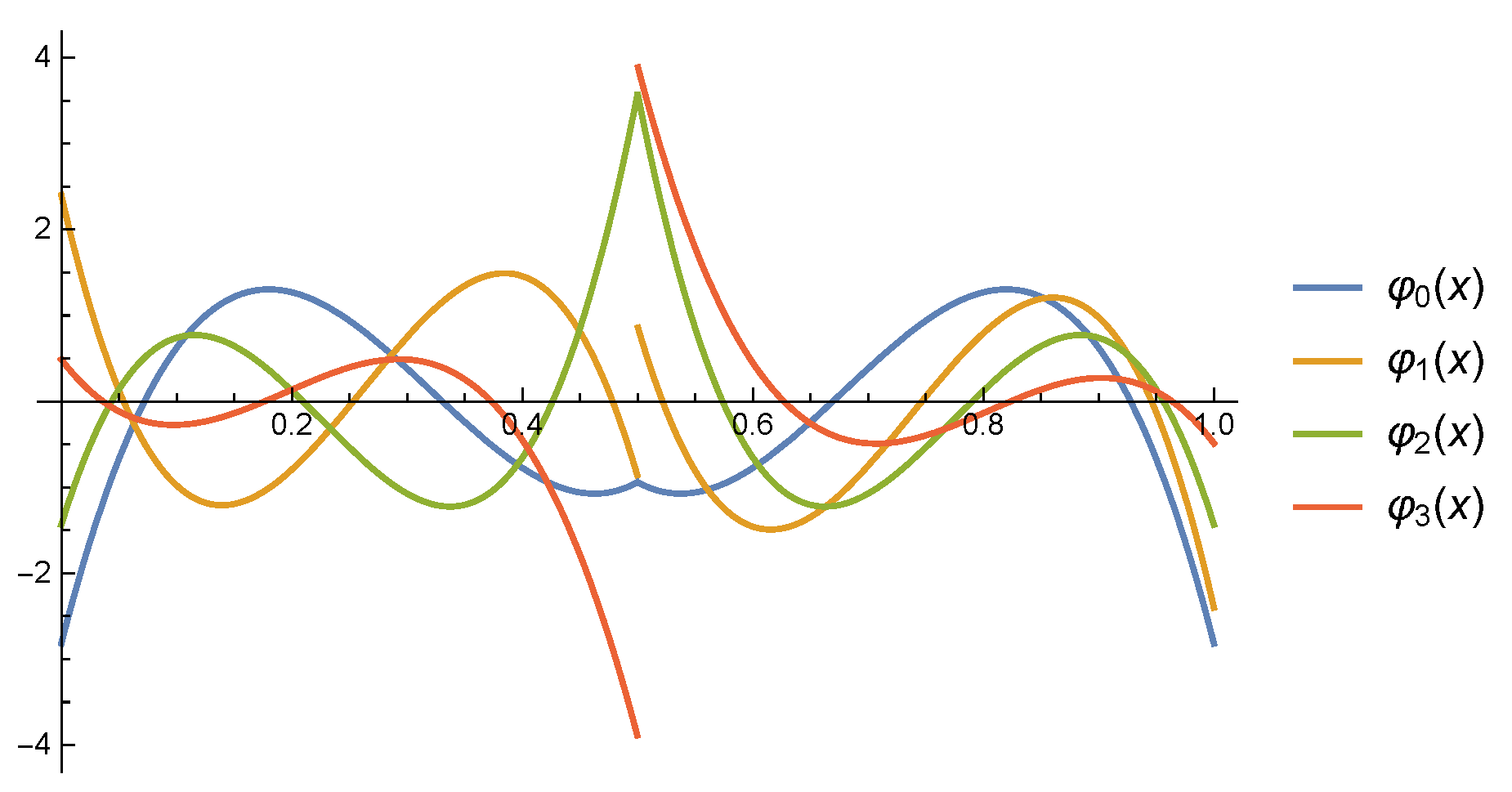
Figure 2.
Network structures used for the incompressible N-S equation (left) and damped wave equation (right). The number of channels for each layer is indicated by the numbers beneath the blue bars.
Figure 2.
Network structures used for the incompressible N-S equation (left) and damped wave equation (right). The number of channels for each layer is indicated by the numbers beneath the blue bars.
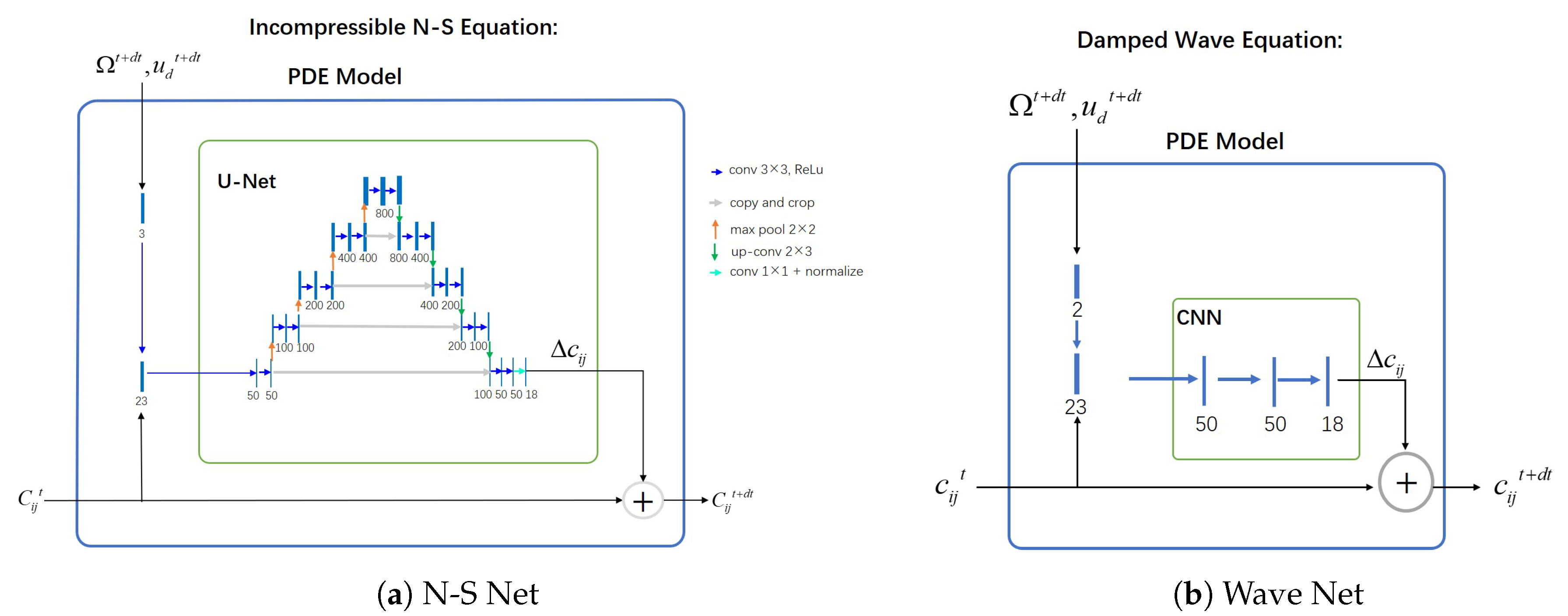
Figure 3.
PDE model pipeline using LMWs. Samples for training and evaluation can be obtained at any point in space and time due to the continuous nature of the solution.
Figure 3.
PDE model pipeline using LMWs. Samples for training and evaluation can be obtained at any point in space and time due to the continuous nature of the solution.
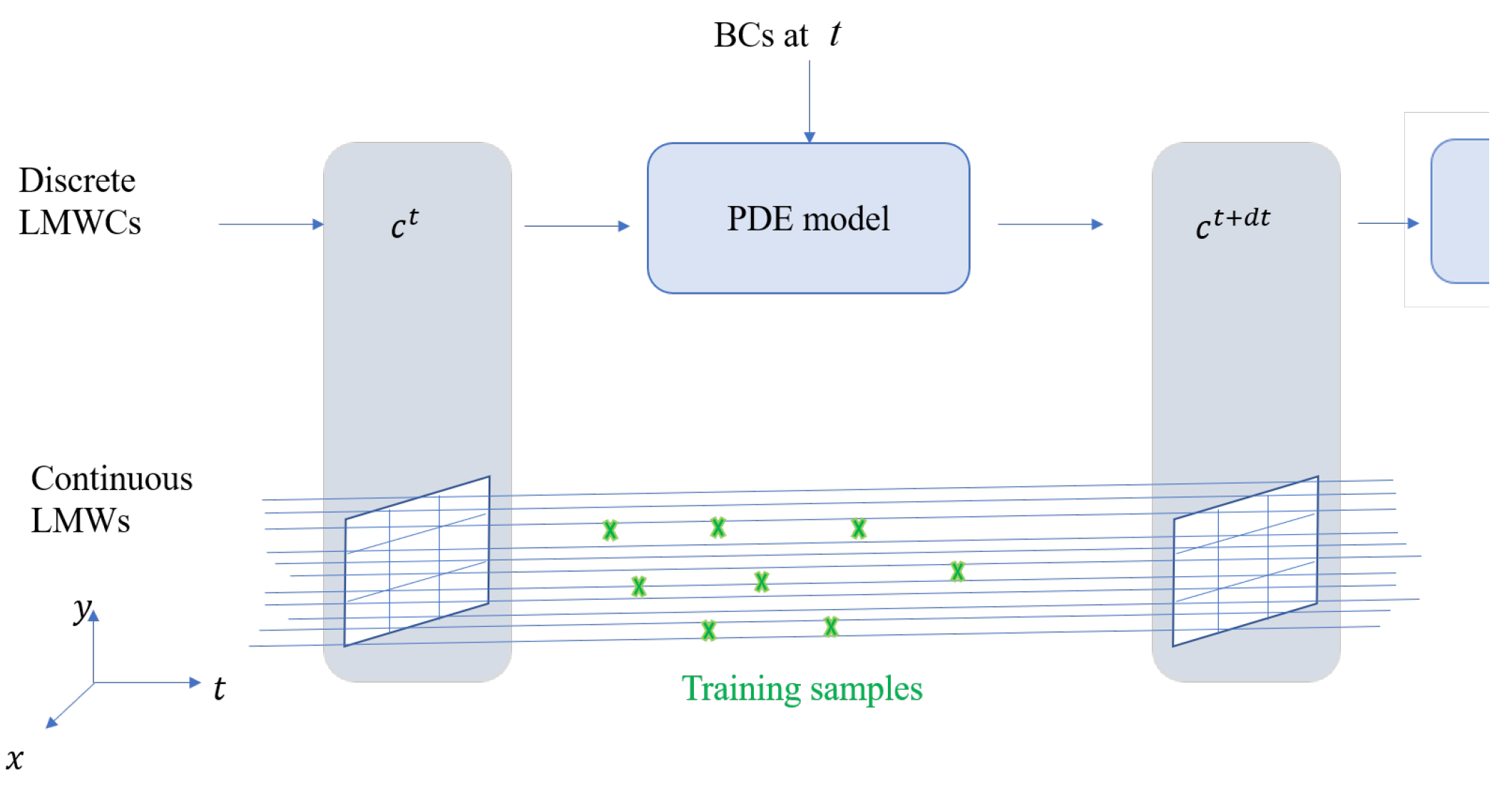
Figure 4.
LMWs are extended as even or odd functions to the interval and zero elsewhere.
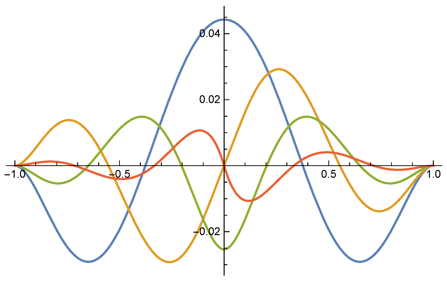
Figure 5.
Training cycle similar to [39].
Figure 5.
Training cycle similar to [39].
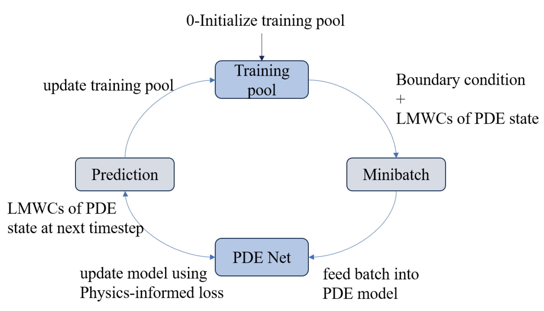
Figure 6.
Stability of solution for damped wave equation.
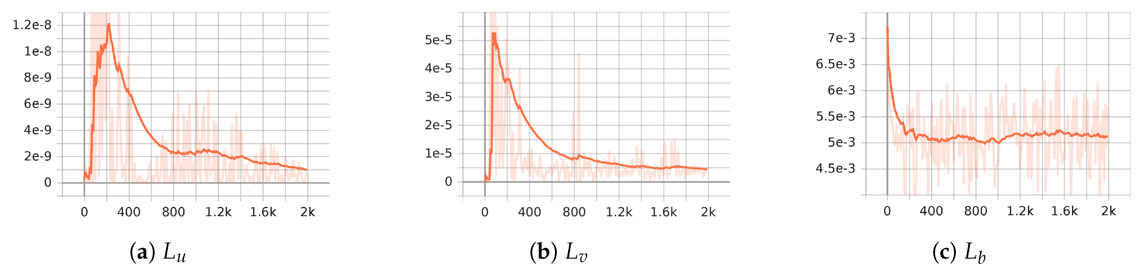
Figure 7.
Stability of PiLMWs-CNN when tackling the N-S equation on the DFG benchmark problem at Re =100.
Figure 7.
Stability of PiLMWs-CNN when tackling the N-S equation on the DFG benchmark problem at Re =100.
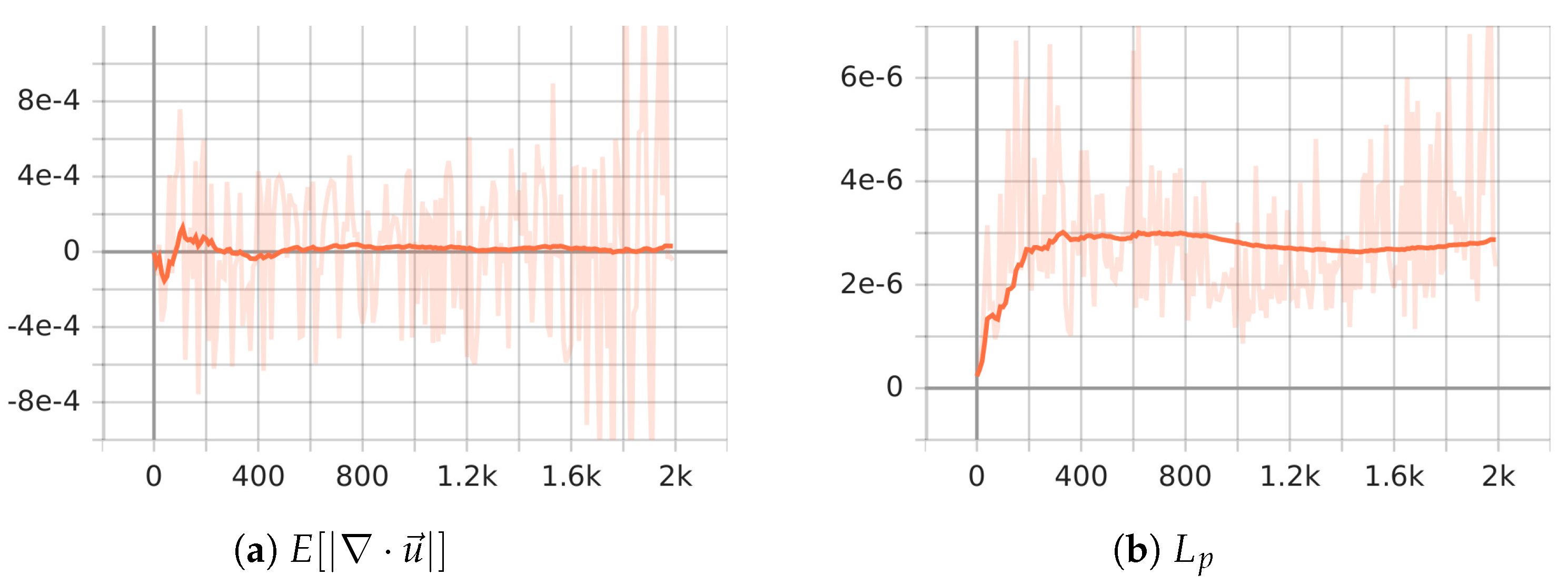
Figure 8.
Stability of PiLMWs-CNN while solving the two-dimensional heat conduction equation.
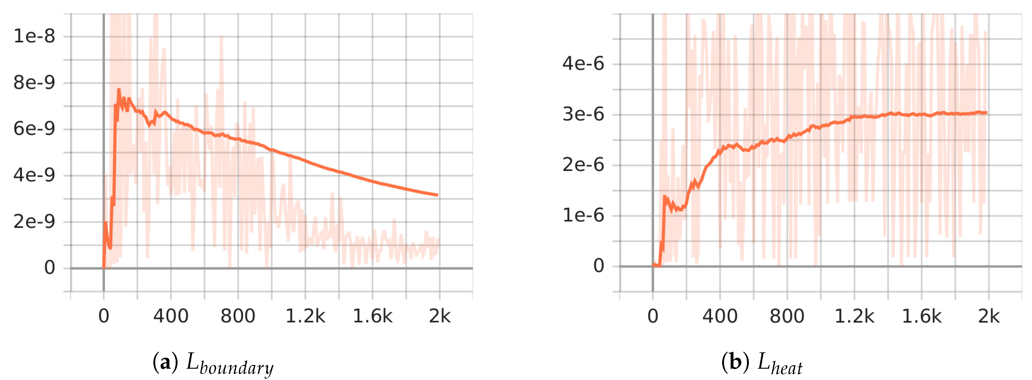
Table 1.
Quantitative results of wave equation.
| Methods | ||||
|---|---|---|---|---|
| Spline Net [11] | 8.511e-02 | 1.127e-02 | 1.425e-03 | |
| 5.294e-02 | 6.756e-03 | 1.356e-03 | ||
| PiLMWs-CNN (ours) | 5.366e-09 | 1.863e-05 | 1.024e-03 | |
Table 2.
Quantitative outcomes for Spline Net, implicit PINN and PiLMWs-CNN at Re=100.
| Methods | ||
|---|---|---|
| implicit PINN | 1.855e-03 | 1.465e-06 |
| Spline Net [11] | 7.492e-04 | 9.04e-04 |
| PiLMWs-CNN(ours) | 5.967e-06 | 2.506e-06 |
Disclaimer/Publisher’s Note: The statements, opinions and data contained in all publications are solely those of the individual author(s) and contributor(s) and not of MDPI and/or the editor(s). MDPI and/or the editor(s) disclaim responsibility for any injury to people or property resulting from any ideas, methods, instructions or products referred to in the content. |
© 2023 by the authors. Licensee MDPI, Basel, Switzerland. This article is an open access article distributed under the terms and conditions of the Creative Commons Attribution (CC BY) license (http://creativecommons.org/licenses/by/4.0/).
Copyright: This open access article is published under a Creative Commons CC BY 4.0 license, which permit the free download, distribution, and reuse, provided that the author and preprint are cited in any reuse.


