Predictive Modelling of Healthcare Insurance Costs Using Machine Learning

1. Introduction

Healthcare spending has increased exponentially worldwide, and there is a strong need for predictive models that can provide insight into the determinants of medical expenses. The ability to effectively predict insurance costs is valuable for both individuals and insurers. For insurers, predictive modeling enables enhanced risk evaluation, leading to better premium estimates. For individuals, having an understanding of how lifestyle and demographic factors influence healthcare expenditure can guide decision-making towards healthier habits and budgeting [1,2].

This study explores the application of data science techniques in evaluating medical insurance spending using machine learning to make predictions of costs based on significant demographic and lifestyle variables such as age, BMI, smoking, and location. Using regression models, this paper attempts to identify the most predictive factors affecting insurance premiums and explore how well predictive models measure medical bills. The conclusions derived from this study have the potential to optimize insurance pricing strategies, enhance policy-making choices, and promote cost-reducing healthcare alternatives[3].

This research t shows how data science can be utilized to solve some of the pressing problems faced in the healthcare sector, namely rising medical expenses. The process involves the use of machine learning and visualisation methods to analyze how demographic, health, and lifestyle factors influence one’s healthcare expenditure. As data science becomes increasingly important to various industries, predictive modelling in the healthcare sector has transformed potential and a great future in promoting decision-making. It also proves that data science applied to a real-world setting is very important in helping various stakeholders, including insurance companies, individuals, and policymakers, make the right decisions regarding economic as well as health matters[4,5,6].

1.0. Background and Project Goal

Over the past decades, healthcare expenditure has increased exponentially across the globe, and hence the need for some predictive models that can explain such high demand for healthcare has increased. The purpose of this project is to leverage data science in creating a reasonable analysis of healthcare insurance premiums and investigate the various demographic and lifestyle determinants of healthcare costs [7,8,9].

The objective of the project is to construct and evaluate predictive models that forecast insurance charges based on specific attributes, which are age, BMI, smoking, and location. The models have applications in many areas. For example, insurance firms may apply them in risk assessment via the computation of the premium value accurately. In addition, people can distinctly see how their lifestyle choices and some demographics play a role in the rates of their health insurance. This enables them to modify their behaviours to prevent higher healthcare costs [10,11,12].

1.2. Background Information

Cost prediction in the healthcare industry is very important for insurers and policymakers to assess financial risk and determine appropriate premiums. As costs grow due to factors such as aging populations, lifestyle changes, and advancements in medical technologies, it is important to outline the factors driving health expenditure. Thus far, machine learning has shown effective performance in expense predictions with age, BMI, smoking status, and regional variations being the crucial variables of shaping risk profiles and premiums.

1.3. Problem Statement

The total population across the globe has been increasing steadily, but this becomes a problem for most of the healthcare systems across the globe. While there are many countries that possess a universal healthcare system that can be extended to all people as long as government spending is adequate, there are other countries where political will is so weak that it becomes a problem for the vulnerable populations.

In particular, the United States of America is the perfect example of one of the handful of countries that lack universal healthcare. With no universal healthcare system in place, many Americans spend as much of their income on healthcare. This is clearly attested when in 2022, Americans will probably spend about $12,555 per capita on healthcare, which is higher than most OECD countries, and has been increasing ever since. (Wager et al., 2024).

1.4. Scope and Limitations

For this project, the dataset used is the Medical Insurance Cost Prediction dataset, created by M Rahul Vyas, and which was last updated in March 2024. The dataset contains many different factors that affect medical costs, such as their age, sex, BMI, whether or not they have children, whether or not they smoke, what region they are from, and insurance costs for them. This information only accounts for those living in the United States, and does not account for other countries, such as Canada or Mexico, both of which have universal healthcare systems.

This framework also does not consider what kind of company the individuals the data they consented to are insured with either. Main questions being posed in the dataset itself are: (i) What are the major factors influencing costs? (ii) How precise are such machine learning models in projecting medical costs? (iii) How would machine learning models help make the insurance firms insuring individuals more effective and profitable?

2.0. Data Set Description

This section explains the dataset of this study in detail. The dataset is central to grasping the problem and highlights the following predictive modeling and analysis. The most crucial information of the dataset, ranging from its collection method, characteristics, quality and reliability and relevant statistical summaries to present a comprehensive insight into the structure, variability and most influential trends of the data, is given below.

2.1. Description of the Dataset

The Medical Insurance Cost Prediction dataset provides crucial data on healthcare expenditure in the United States. The dataset assists insurance companies in creating machine learning models for cost prediction as well as identifies essential determinants of costs. Analyzing these factors, insurance companies can introduce better pricing mechanisms and also better risk management techniques. This in turn makes their premium calculation more precise and business decisions more efficient.

2.2. Data Collection Method

Despite the lack of information regarding how the data was gathered, the dataset includes important features that impact healthcare expenses, including demographic features (age, sex, number of children), health factors (BMI), lifestyle factors (smoking status), geographic factors (region), and the associated insurance costs. Additionally, the dataset’s richness allows for the scrutiny of the manner in which various factors interact to impact medical expenses. Furthermore, the structure of the dataset records quantitative and qualitative variables, which allows researchers to examine correlations and patterns within the data. The presence of a broad range of influential variables offers a solid basis for predictive modelling that can successfully predict medical insurance costs [9,10,11].

This dataset contains quantitative and qualitative measures. The heterogeneous data structure allows predictive models to draw conclusions about the effect of each variable on the total cost. By considering continuous measures along with categorical categorizations, the data set formulates an inclusive way of conceiving insurance cost variation [12,13,14].

Body Mass Index (BMI) is one of the significant features in the data as it informs us about an individual’s body composition and is a very important indicator of health risk. BMI is typically calculated from an individual’s weight and height measurements by using the formula:

BMI = Weight (kg) / Height (m)^2

In this formula, weight is in kilograms (kg) and height in metres (m).

The BMI values are usually categorized to assess the health risk associated with body weight. As BMI increases, there tends to be a rise in healthcare need and spending. The measure that is calculated is handy for examining associations between an individual’s body frame and his or her insurance premiums within the data.

2.4. Data Quality and Reliability

The data set is well formatted with defined columns and restricted permissible data types. Nevertheless, it is also critical to test and validate data quality for outliers that can cause a skewed output such as missing or inconsistent data. Nonetheless, any potential outliers, particularly in continuous variables such as BMI and age, need to be closely monitored since they are likely to skew the predictions created by the model. A big limitation is that the dataset is only a limited snapshot to the enormous set of health-related variables which may not provide the complete picture of what contributes to medical expenses. Insurers may decide to look at other drivers which are not observable in this dataset such as blood work tests: White blood cell (WBC) count, red blood cell (RBC) count, Haemoglobin (Hgb) test, and many more (Care Health Insurance, 2023).

Additionally, the “region” variable classifies people into very restricted location choices: northwest, northeast, southwest and southeast of the United States of America. The approach has the problem of oversimplifying geographic variations in healthcare expenses. Furthermore, the “yes” or “no” option for the variable “smoker” limits the observation. This limits the observation because it excludes the people who previously smoked. For instance, a person who has managed to quit smoking can still have increased health risks or medical expenses as a result of previous smoking habits, but this would not be indicated in the current “yes” or “no” status. There is also the possibility of response bias, where a person gives a false indication of their smoking status, either deliberately or inadvertently, thereby distorting the relationship between smoking and insurance premiums [15,16,17].

The figures are sourced from Kaggle and not officially validated by hospitals or healthcare professionals. Therefore, one must question the extent to which this information is current and representative of actual health spending trends in the real world. However, it has a higher level of legitimacy because the data are copyrighted by the Massachusetts Institute of Technology (MIT) and therefore give legitimacy to the premise and probable accuracy. This copyright mark enhances the validity of the dataset for academic and research purposes [18,19]. But the data must be utilized with caution over its limitations and in general perspective of health cost heterogeneity [20,21,22].

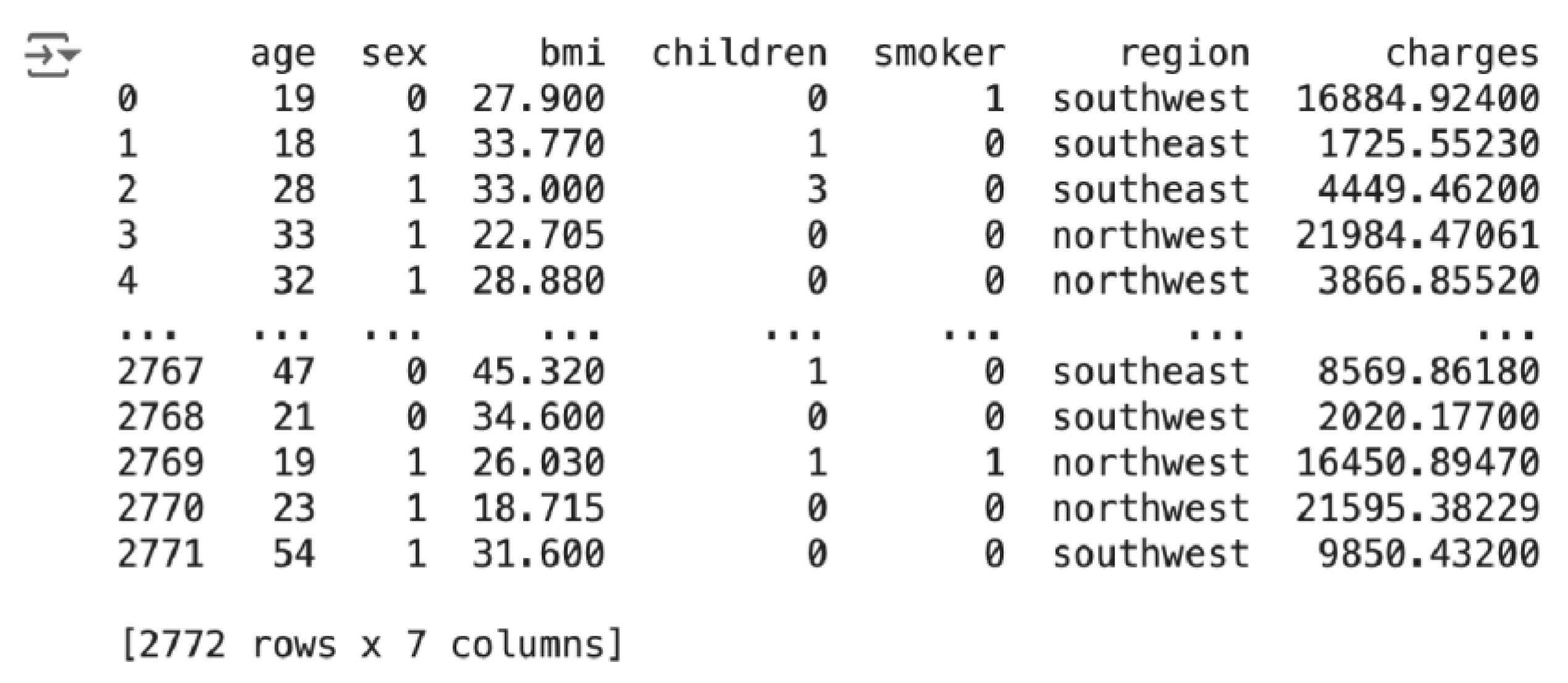
2.5. Data Examples

Based on the first row of the data sample, one can interpret a data record as: the patient is a 19-year-old female with BMI 27.9, no children, a smoker and living in the southwest area, with medical insurance expenses of approximately $16,884.92. The second record can be read as: the individual is an 18-year-old male with a BMI of 33.77 who has one child, does not smoke and lives in the southeast region, with medical insurance charges of approximately $1,725.55.

Table 1. Snippet of data from dataset.

age	sex	bmi	children	smoker	region	charges
19	female	27.9	0	yes	southwest	16884.924
18	male	33.77	1	no	southeast	1725.5523

Table 1. Snippet of data from dataset.

age	sex	bmi	children	smoker	region	charges
19	female	27.9	0	yes	southwest	16884.924
18	male	33.77	1	no	southeast	1725.5523

2.6. Statistical Summaries

This part of the paper will discuss the properties of the dataset such as important summary statistics to further understand the central tendency and variability of the data. Histograms and box plots visualisations will illustrate the distribution of values, patterns, ranges, and any potential outliers. These statistical summaries and visualisations together give important insights into the structure of the dataset for subsequent analysis and modelling. To start with, the key summary statistics for the data set focuses on the important numerical measures like mean, median, and standard deviation. The following table presents the central tendencies and distribution of every numerical variable in the data set, namely age, BMI, children, and charges [21,22,23,24].

Table 2. Statistical Summary Table.

Table 2. Statistical Summary Table.

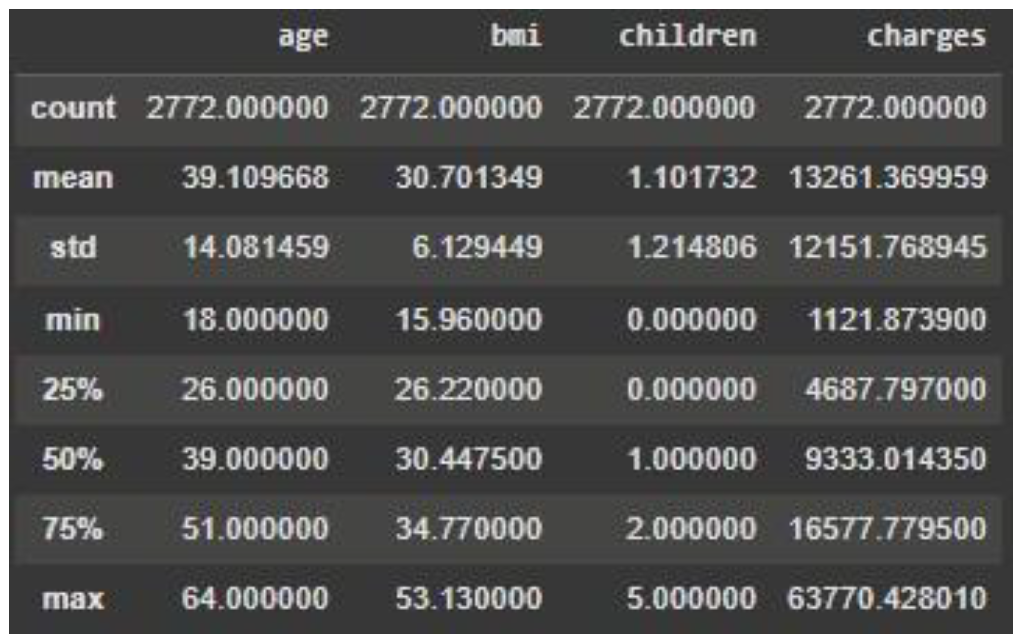
Each column has data for 2,772 records, meaning there are no missing values in these columns. The mean shows the average age of the sample is 39.1 years, for BMI is 30.7, for the number of children is 1 and the average cost is $13,261. The standard deviation shows the variance of each feature. The standard deviation of the age attribute is 14.1 years, reflecting a wide range of ages in the data, and charges have a high standard deviation of $12,151, reflecting a wide range of medical charges. The min and max provide the range of each attribute. For example, the range of age is from 18 to 64, and charges range from $1,121.87 to $63,770.43, reflecting an extremely wide variety of medical expenditures.

Plots of these distributions in histograms and box plots highlight other patterns, such as the uniform distribution of age peaking between 20 and 40 years, a bell curve distribution of BMI peaking at 30, and a highly right-skewed distribution of medical charges, which captures that most individuals have low medical costs while a small group has far higher costs. An insurance charge box plot illustrates the stark difference between non-smoker and smoker charges [27,28], highlighting the impact of smoking on health care expenditure. In addition, a correlation heatmap shows a moderate, positive correlation between charges and age (0.30) and a weaker correlation between charges and BMI (0.20), which suggests that while age and BMI partially explain medical expenditure, something else is more important. A scatter plot better depicts the expense of smoking, which is that smokers, particularly the higher-BMI ones, have much higher insurance premiums compared to non-smokers. The findings emphasize the importance of considering demographic and lifestyle factors in predictive modelling for healthcare cost prediction.

Figure 1. Percentage of Categorical Features.

Figure 1. Percentage of Categorical Features.

Figure 2. Visualisation of Categorical Features.

Figure 2. Visualisation of Categorical Features.

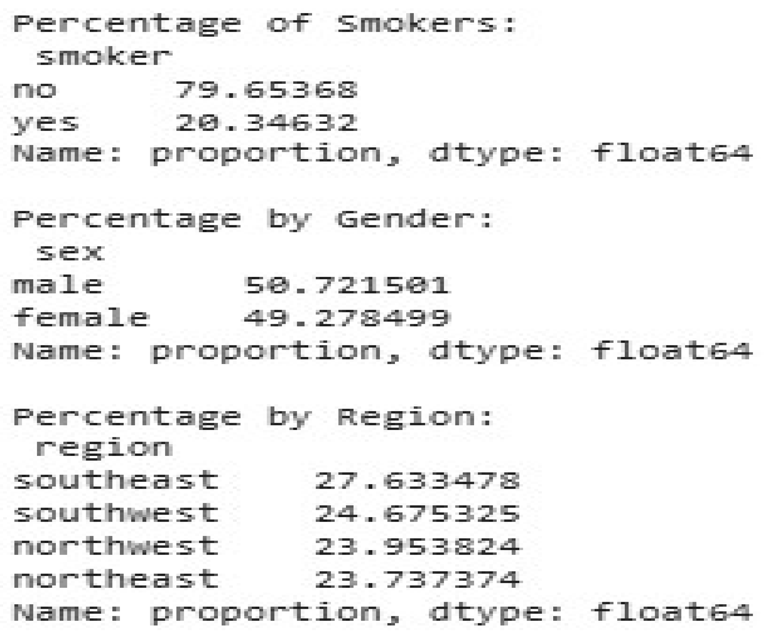
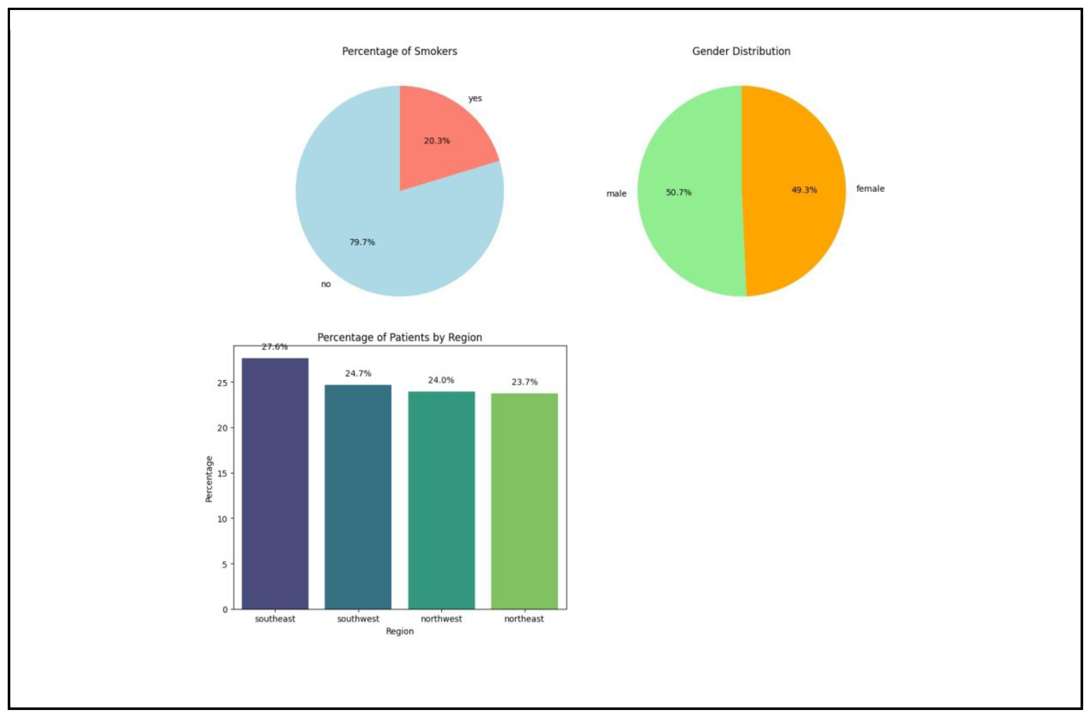
The following categorical distributions provide further information about the background of the data. Nearly 79.65% are nonsmokers and 20.35% are smokers, representing a plurality of nonsmokers in the sample, which can have a skewed effect on mean medical expenses. The gender attribute is evenly distributed. 50.72% of the records are male and 49.28% are female, representing a fair comparison between genders. The data is also balanced by region. There are 27.63% southeast individuals, 24.68% southwest individuals, 23.95% northwest individuals, and 23.74% northeast individuals, so it is a balanced regional comparison.

2.6. b Categorical Distribution

A histogram may represent the distribution of continuous numerical features. This visualisation approach illustrates the distribution of data over various values, highlighting concentrations and probable skewness.

Figure 3. Distribution of Categorical Features.

Figure 3. Distribution of Categorical Features.

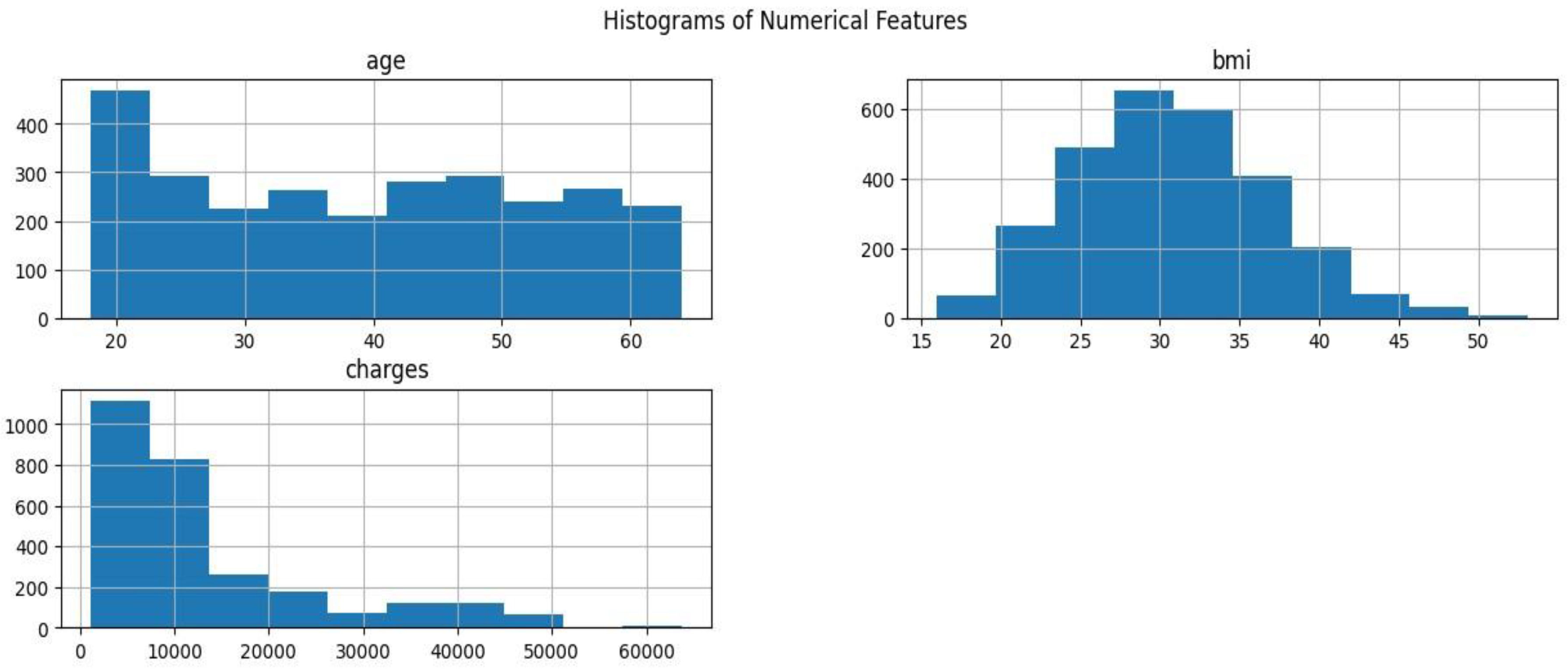
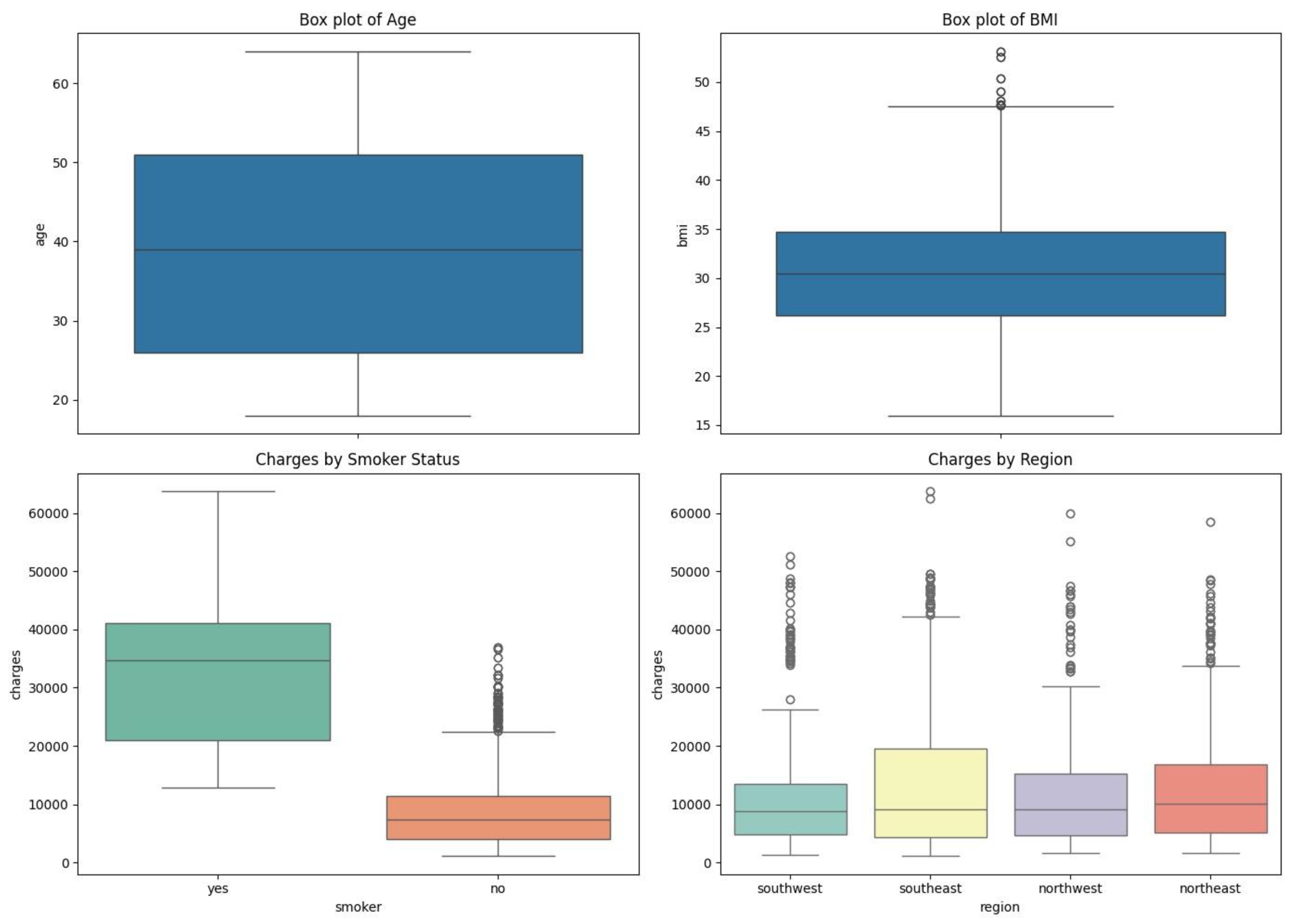
A histogram can represent the distribution of continuous numerical attributes. This visualization technique illustrates the distribution of data across various values, highlighting concentrations and probable skewness. The age feature histogram is evenly spread throughout the adult age group, with a higher concentration of people aged 20 to 40 years. The sample is mostly comprised of young people, with a bias for the younger age groups, but older age groups are well represented. The BMI histogram shows a bell-shaped distribution with the mean centered at about a BMI of 30. The distribution is a typical set of BMI values in the larger population, and there are no outliers or skew. For charges, the histogram shows an extreme right skew, with the majority of people with lower medical charges and a few with significantly larger charges. This asymmetry indicates that additional exploration of the features in (or outside of) the data set may yield valuable information on the determinants of the lower insurance coverage. These features were also visualized as box plots to understand the distribution of numeric features age, bmi, and the distribution of charges by smoker status and region.

Figure 4. Box-Whisker Plot of Features.

Figure 4. Box-Whisker Plot of Features.

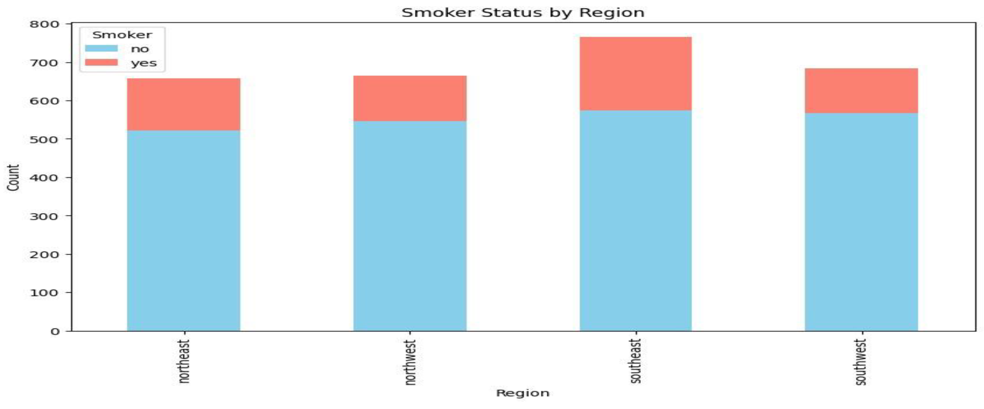
The box plot of BMIs indicates that BMIs are clustered around a median of 30 with few outliers greater than 40. This suggests that, while the majority of people have a BMI within a typical range, an infinitesimally small fraction have very high BMIs. The box plot of insurance premiums by smoking status indicates a considerable cost disparity between smokers and non-smokers. Smokers possessed a higher median and range than the non-smoker. Finally, the region by charges box plot illustrates the same pattern of charges over the four regions with minor variation across them. In addition, smokers’ rate in different regions can be depicted as a stacked bar chart to describe the prevalence of smoking status in different places.

Figure 5. Stacked Bar Chart for Smoker Status by Region.

Figure 5. Stacked Bar Chart for Smoker Status by Region.

Every bar is representative of an area, with smokers in pink and non-smokers in blue having separate sections. The southeast area has the largest total number and a marginally larger percentage of smokers than the other areas, whereas the other areas all have a roughly equal number of smokers and non-smokers.

2.6. Correlation Visualisations

A correlation heatmap will represent the correlation between numeric features age, BMI, and charges. This enlightens the study to take into account related elements.

Figure 6. Correlation Heatmap of Age, BMI and Charges.

Figure 6. Correlation Heatmap of Age, BMI and Charges.

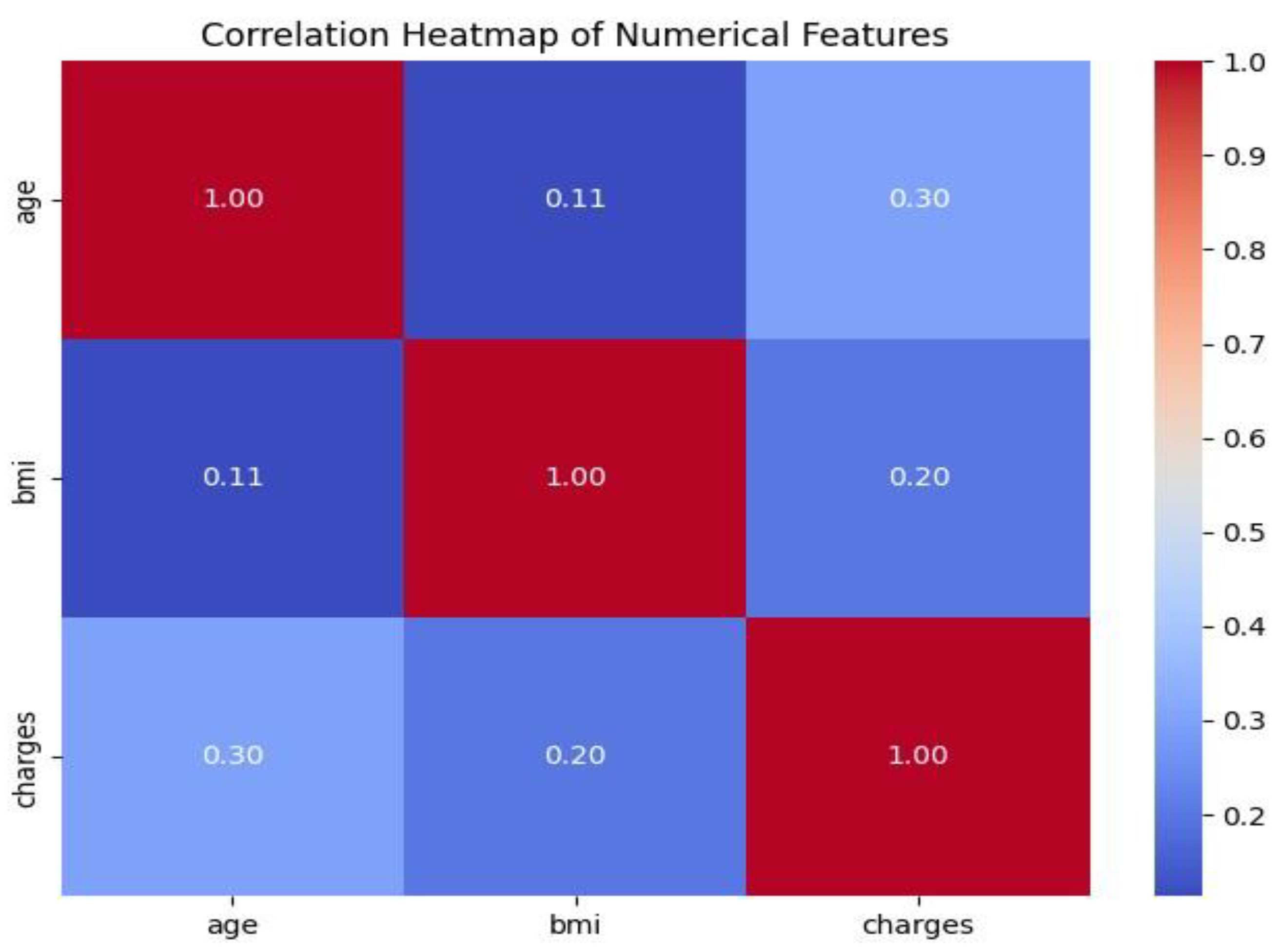
The diagonal values, in which each attribute is correlated with itself, demonstrate a perfect correlation of 1.00 and serve as benchmarks for heatmaps. There is a positive correlation of 0.30 between charges and age, which indicates that insurance charges rise with age, but other factors are most likely to influence total charges. The correlation between BMI and charges are weaker, at 0.20, indicating a generally positive relationship. This means that those with a greater BMI may have slightly greater medical costs, but this impact is very small.

Figure 7. Scatter Plot of Charges Against BMI by Smoker Status.

Figure 7. Scatter Plot of Charges Against BMI by Smoker Status.

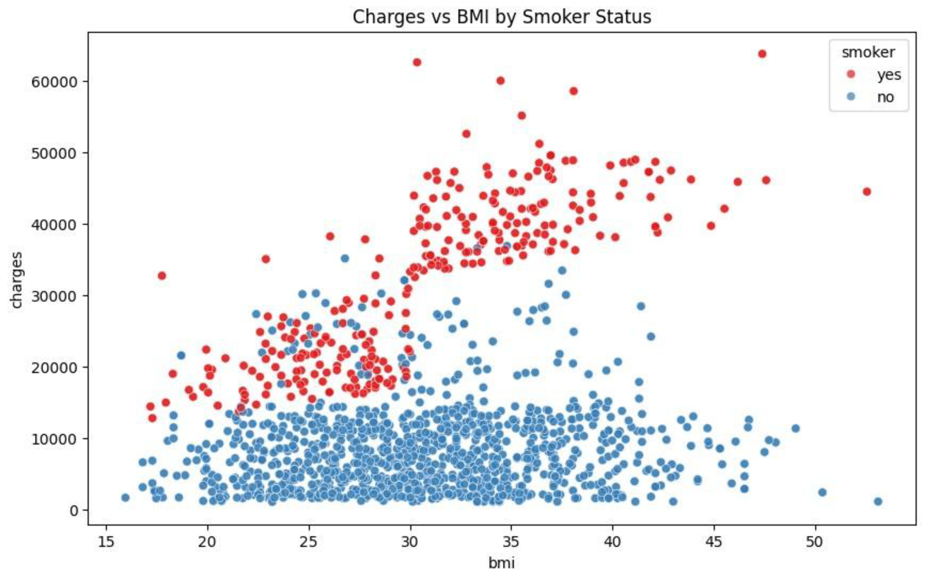
The relationship between smoker status, charges and BMI can be plotted with scatter plot. In this, the blue dots represent the non-smokers in the sample data and the red dots represent the smokers.

Figure 7 - Scatter Plot of Charges vs. BMI by Smoking Status. The figure illustrates a wide difference in insurance fees among nonsmokers and smokers. Smokers incur more, particularly at greater BMI levels, as evidenced by the concentration of red dots at the upper region of the figure. This indicates that smoking contributes greatly to medical bills, especially at increasing levels of BMI. Nonsmokers (blue dots) incur lower fees, with charges remaining roughly constant at various levels of BMI. The smokers and the individuals with a higher BMI have a higher likelihood of facing significantly higher insurance rates. The clear cost difference between smokers and nonsmokers highlights the economic impact of smoking on healthcare.

3. Proposed Methodology

3.1. Research Design

This study employs a predictive modeling framework to predict healthcare insurance spending on the basis of population and lifestyle variables. A machine learning regression approach using data-driven methods will be utilized to identify the most significant cost drivers and validate the performance of models.

3.2. Data Collection

The study will work with the publicly available Medical Insurance Cost Prediction dataset on Kaggle, created by M Rahul Vyas. The dataset includes patients’ records with features such as:

• Age
• Gender
• Body Mass Index (BMI)
• Number of Children
• Smoking Status
• Geographic Region
• Insurance Charges

All this data will be used to train, validate, and test machine learning algorithms.

3.0. Data Preprocessing and Issues

The second process after submitting the description of the provided dataset is data preprocessing of the data. Data in the dataset must be pre-processed to improve data quality and standardize it, meaning finding some missing values in the dataset or correcting incorrect data due to incorrect formats or incorrect input. It also helps to achieve maximum performance for predictive modelling, improves efficiency and reduces complexity with guaranteed standardised formats and values and encoding variables as most models work best with binary, numeric data.

This data processing step shows three major data preprocessing methods, namely binary encoding, detection and processing outliers and standardisation. Binary encoding allows the conversion of variables to the binary 0 and 1 values representing negative and positive values respectively, depending on context, in order to aid dimensionality reduction in an attempt to prevent overfitting and sabotaging the predictive model(Bolikulov et al., 2024).

Data sets may contain observations which seemed to be out of context from the entire observation within it, and thus these outliers need to be removed since these affect the performance of the model and the impact will be observed in data quality. Outliers have a negative effect on data analysis and contribute to low validity in statistics and offer poor insights in the exploratory data analysis case.

In order to offer better performance in the predictive machine modeling, best practice for optimal performance, interpretability and numerical stability is standardizing the data set by feature having mean 0 and standard deviation 1. Standardizing brings points of a feature into the center of mean 0 and scaled comparatively with variance. Standardization is necessary for the dataset since attributes such as “smokers” are scale-sensitive and it is reliant on the relationship between the BMI of the smokers and charges due to their ailments caused by their smoking habit.

3.1. a Binary Encoding and One-Hot Encoding

Since most machine learning models can accept numerical inputs alone, the categorical attributes in this dataset must be converted into binary or numerical format. Binary encoding is applied on categorical attributes sex and smoker. Both are two-valued categorical variables - ’smoker’ has yes and no, and ’sex’ has male and female. Binary encoding helps to convert such features into binary numbers, i.e., 1 or 0, and both of them are extremely suitable for model training due to this. It helps ensure that machine learning models can process and preserve their original meaning in the appropriate manner without introducing any hierarchical or ordinal relationships among these categorical values.

Figure 8. Binary Encoding Sex and Smoker Features.

Figure 8. Binary Encoding Sex and Smoker Features.

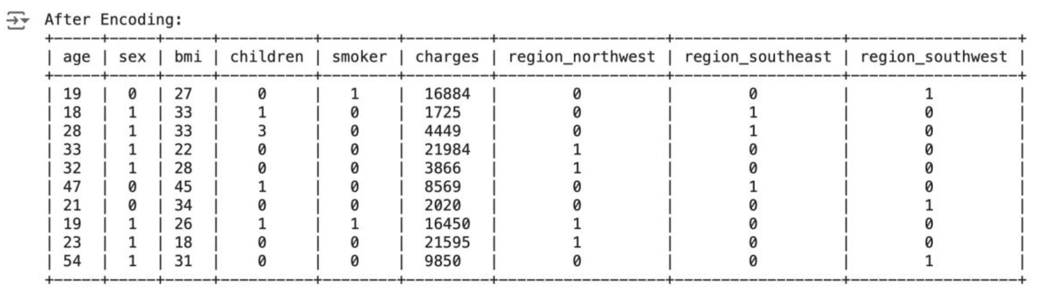
Here, “yes” is substituted by 1 and “no” by 0 in the smoker column, and “male” is substituted by 1 and “female” by 0 in the sex column using the.map() function. Hence, the smoker and sex columns are prepared to be used as model input as they have only binary values.

Region is the other categorical variable in this data that must be encoded. One-hot encoding is used instead of binary encoding because region has several different categories, i.e., northwest, southeast, and southwest with no ordinal or hierarchical relationship between them. One-hot encoding enables each category to be represented by respective binary columns, transforming each region category into different features without implying any order or ranking.

Figure 9. One-Hot Encoding Region Feature.

Figure 9. One-Hot Encoding Region Feature.

One-hot encoding is applied to the region column of df using pd.get_dummies here. For redundancy removal, the initial dummy column is dropped with the parameter “drop_first=True.” The subsequent True and False values are converted to 0s and 1s using the “.astype(int)” function.

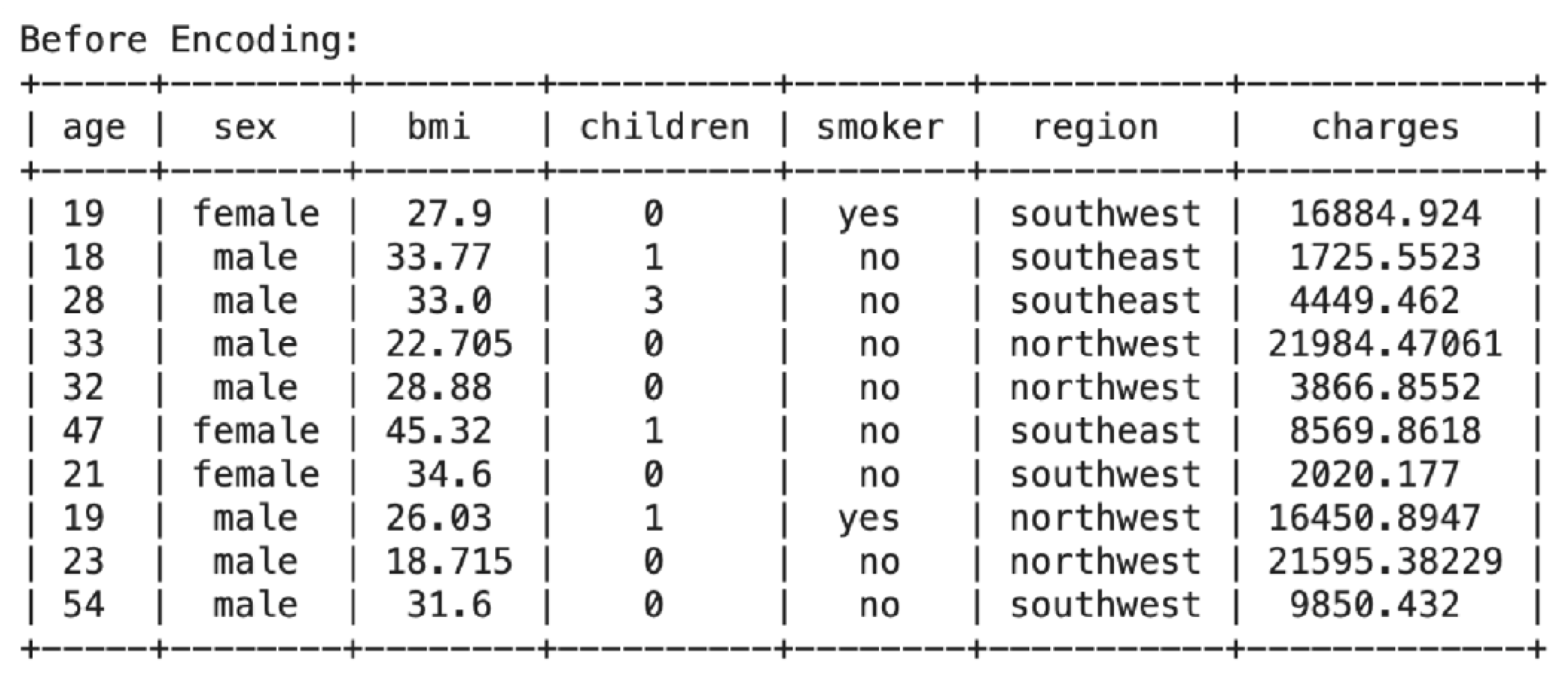
3.1. b Before Encoding

The tabulate function, which is imported from the tabulate library, is used to print the data frame in order to uncover the pre and post-binary and one-hot encoding difference. The first five rows and the last five rows of the dataset are printed using df.head() and df.tail(), respectively. From the above table, it is easily evident that the sex and smoker columns are encoded as strings (“male” and “female”, ‘’yes” and “no”). In the region column, several distinct categories (e.g., “northwest”, “southeast”, “southwest”) are encoded as text labels..

Figure 10. Before Encoding Dataset.

Figure 10. Before Encoding Dataset.

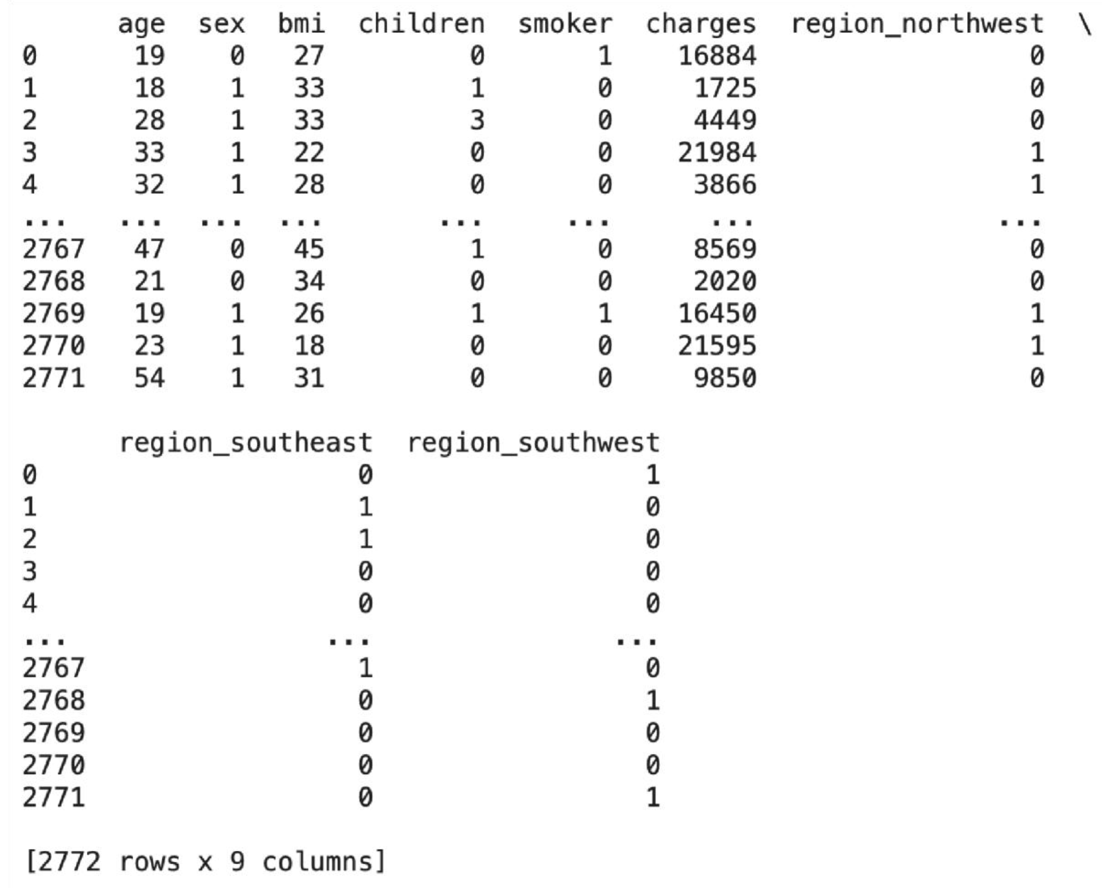
3.1. After Encoding

The following table shows the first and last 5 rows of the data after binary coding has been applied, with the sex and smoker columns encoded. The data in both columns is now in a binary format of 1’s and 0’s. One-hot encoding is also applied to the region column, with different columns for each unique region category, represented in the form of 1’s and 0’s. This ensures that the categorical features for all of the data, since sex, smoker, and region are categorical in nature, get encoded and support the machine learning model.

Figure 11. After Encoding Dataset.

Figure 11. After Encoding Dataset.

3.2. Spotting and Managing Outliers

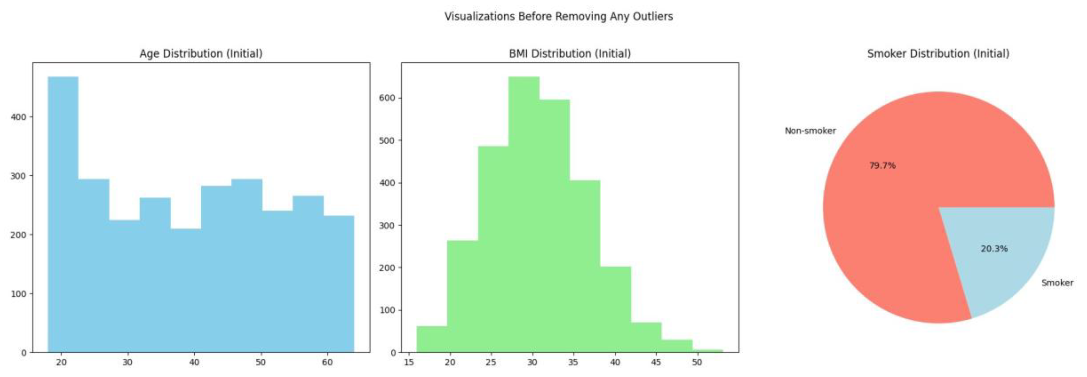
Earlier in this paper, numerical attributes were plotted into histograms to check for potential outliers. The age feature contains high density of values between 18 and 25, as evident from the above code and image. This skew can lead to bias in the analysis. The disproportionately large quantity of smokers can also impact the outcome. The histogram of BMI is a bell curve, which signifies an even overall distribution. This preprocessing step will eliminate outlier data where BMI is higher than the upper quartile, age is below 25, and the subject is a non-smoker. Hence, records of non-smokers aged 18 to 25 years will be eliminated to balance the dataset without drastically affecting the distribution of BMI.

Figure 12. Visualisation Before Removing Outliers.

Figure 12. Visualisation Before Removing Outliers.

Outliers in the BMI characteristic can be found by creating a new data frame containing the BMI data for people below 25 years of age. The upper limit of standard values is then determined using a standard method of finding outliers:

Upper Bound = Q3 + 1.5 X IQR

where Q3 is the third quartile and IQR is the interquartile range.

The result provides the upper limit for non-outlier BMI values for individuals less than 25 years old. Removing non-smoking observations with BMI greater than this upper limit will yield a more evenly balanced sample of smokers, which in turn decreases skewness.

The following code lines will test the deletion of outliers by comparing the size of the data frame before and after eliminating such records.

Four records that met the required criteria were successfully excluded from the dataset. The data included individuals under 25 years of age with a BMI exceeding the computed upper limit of 47.3, who were also non-smokers. Eliminating these outliers mitigates skewness in the dataset by equilibrating the distribution of smokers and non-smokers, especially among the younger demographic.

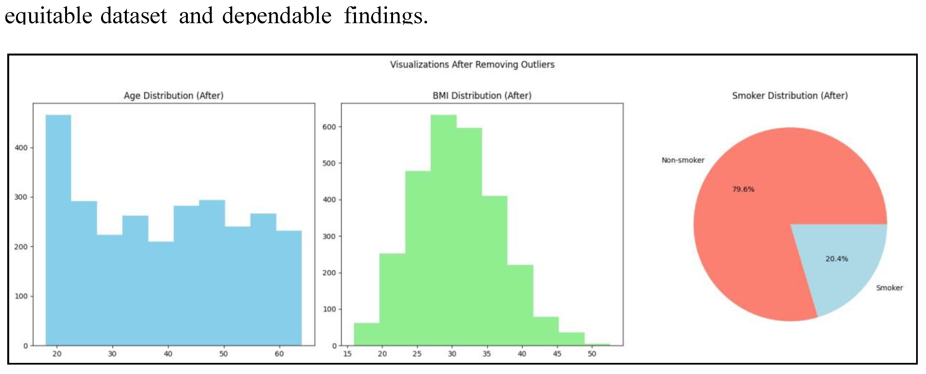
Figure 13. Visualisation After Removing BMI Outliers.

Figure 13. Visualisation After Removing BMI Outliers.

Visualisations indicate a 0.1% rise in smoking prevalence but the age distribution is unchanged, which means data cleansing is needed to fix imbalances in the dataset.

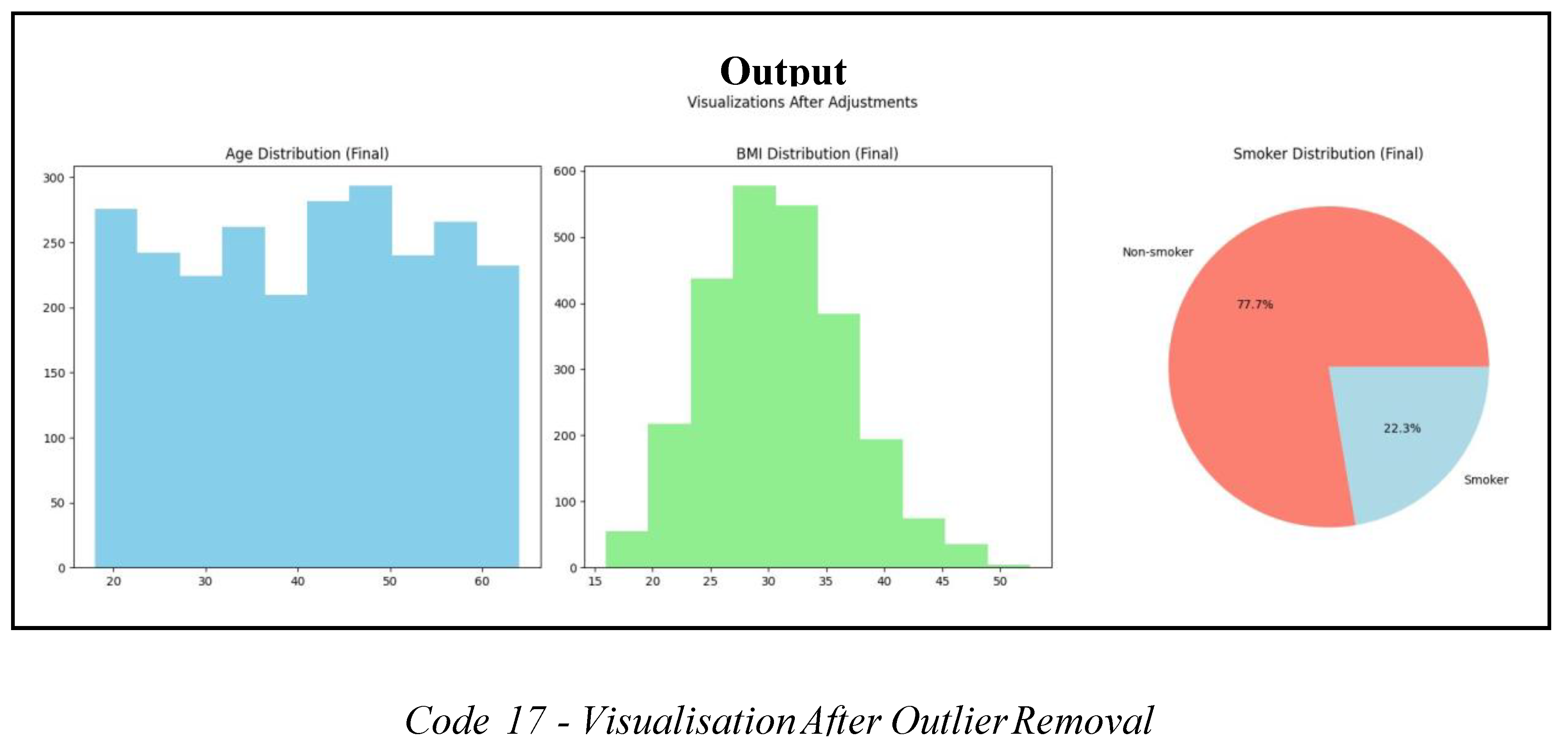
To decrease the number of individuals in the age group 18 to 25 and to have an equitable distribution of non-smokers, an arbitrary number of non-smoker records will be deleted. This is done with the aim of producing a more equitable distribution of age and smoking status, hence removing potential biases in the analysis.

The first procedure is to screen the current non-smoker and smoker statistics in the population younger than 25 years to determine that the elimination process has been successful.

The second procedure entails a random selection of 240 non-smokers’ records ranging from the ages of 18 to 25 years, which will be discarded. This will enable the balance of individuals within this age category with other population categories. A data frame will be created that includes only non-smokers who are less than 25 years old. The random.seed() method will be used to ensure reproducibility by randomly choosing 240 records to delete. The use of a seed allows the repeated replication of this deletion operation, making it easier to achieve better results and verify results.

This method will tactfully balance the dataset, especially in the age group of 18 to 25 years, without sacrificing the distribution of BMI or creating additional biases by an over-sampling of non-smokers.

The code reduced non-smokers younger than 25 from 240 to 218, reducing the bias resulting from over-representation in the age group of 18 to 25. Data is now set for re-estimation with visualisation where the age distribution, BMI, and smoking statuses are investigated so that data cleansing has levelled out the mentioned parameters without skewing the BMI distribution drastically. The following visualizations will give a more accurate representation of the dataset structure, enabling objective research and sound conclusions.

Figure 14. .

Figure 14. .

3.3. Standardisation

Numerical attributes in the data (age, bmi, children) are of different ranges. This is problematic for model training that includes scale-sensitive models such as Linear Regression and Gradient Boosting. Having features with different scales, larger-ranged features may dominate learning and hence result in poorer performance. Therefore, standardisation solves this issue by transforming the numerical features to a common scale with a mean of 0 and a standard deviation of 1 (Sharma, 2022). It makes all the features equally influential on the model, improving its learning efficiency and allowing it to discover optimal solutions more effectively.

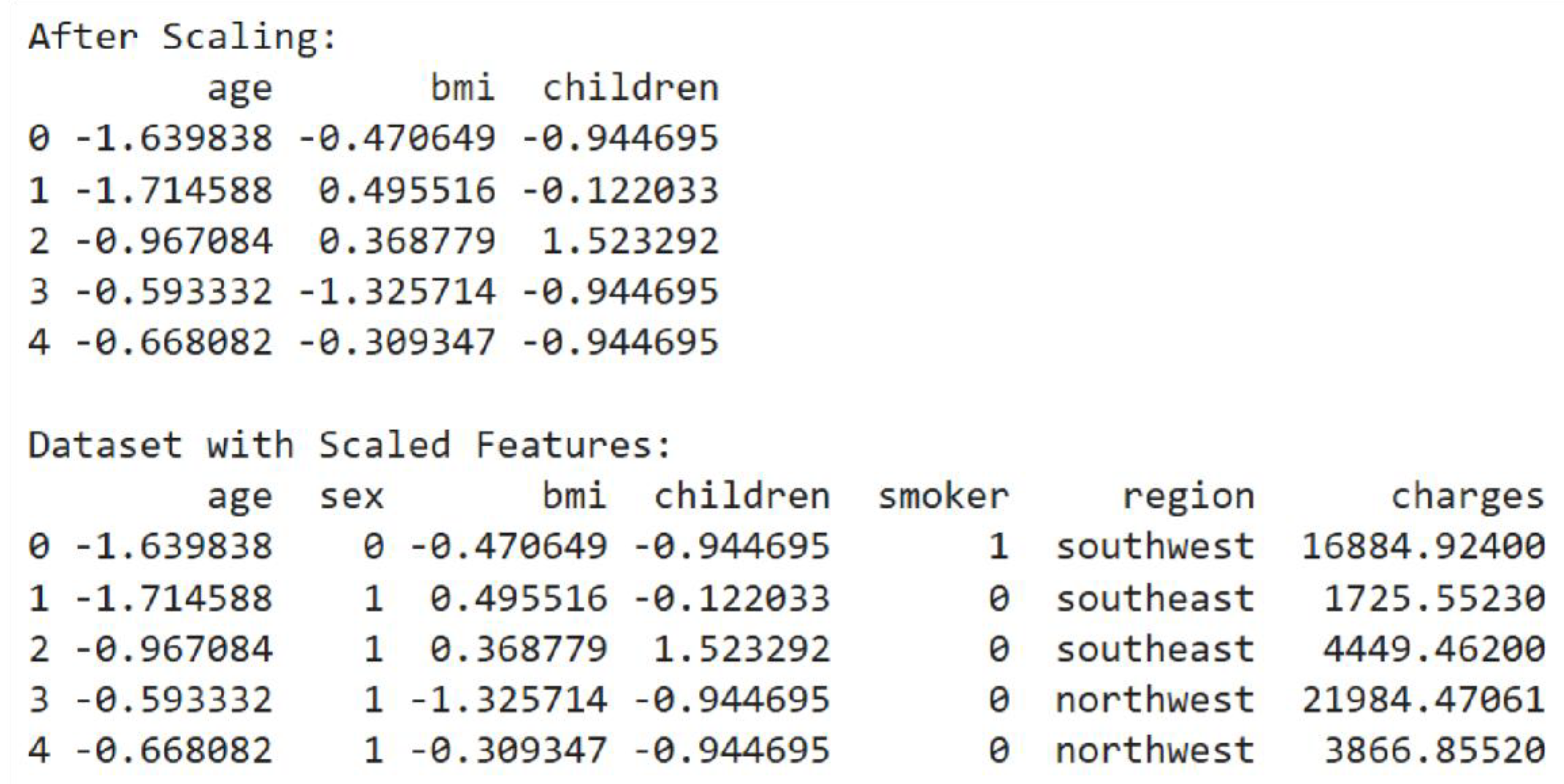
In the code, ‘age’, ‘bmi’, ‘children’ will be standardised. Before applying scaling, the code prints the first five rows of these features to show their original values.

Figure 15. Prior to Scaling.

Standardisation is done by deriving numerical features from the original DataFrame. StandardScaler is used for standardising each feature individually. StandardScaler calculates the mean and standard deviation of every numerical feature. On computation, StandardScaler scales off the mean and normalises to unit variance. The original DataFrame is replicated in order to keep the target variable and other unscaled features. The resulting data set shows standardized numerical attributes, which have been scaled to have mean zero and a standard deviation of 1, so the data set is more appropriate for machine learning algorithms.

Figure 16. After Scaling.

Figure 16. After Scaling.

Standardized data moved in the direction of zero, and values are scattered as per how far they were from the mean. Points which are below the mean are labeled by negative numbers, and points above the mean are labeled by positive numbers.

4.0. Data Science Techniques

There are several data science methods which can be employed to investigate data sets. This study is seeking to forecast insurance costs based on three various models of machine learning by employing the regression models of the extensive ’sklearn’ library: Linear Regression, Random Forest Regressor, and Gradient Boosting Regressor (Fitri, 2023).

4.1. Linear Regression

Linear Regression builds a simple model. It is interpretable and can indicate if there is a linear relationship between variables and outcomes. Although it may not depict complex relationships, it provides a good foundation.

4.2. Random Forest Regressor

Random Forest Regressor technique is effective with non-linear interaction and doesn’t demand expensive preprocessing such as scaling. It is comparatively overfitting robust because it can potentially average groups, and can give feature importance scores which assist in identifying key predictors of insurance premiums.

4.3. Gradient Boosting Regressor

The Gradient Boosting Regressor works especially well in regression scenarios with intricate data patterns. Through constant error correction, it is capable of potentially detecting intricate correlations in the data. It may, however, potentially require exact tuning to prevent overfitting.

4.4. Implementation of Models

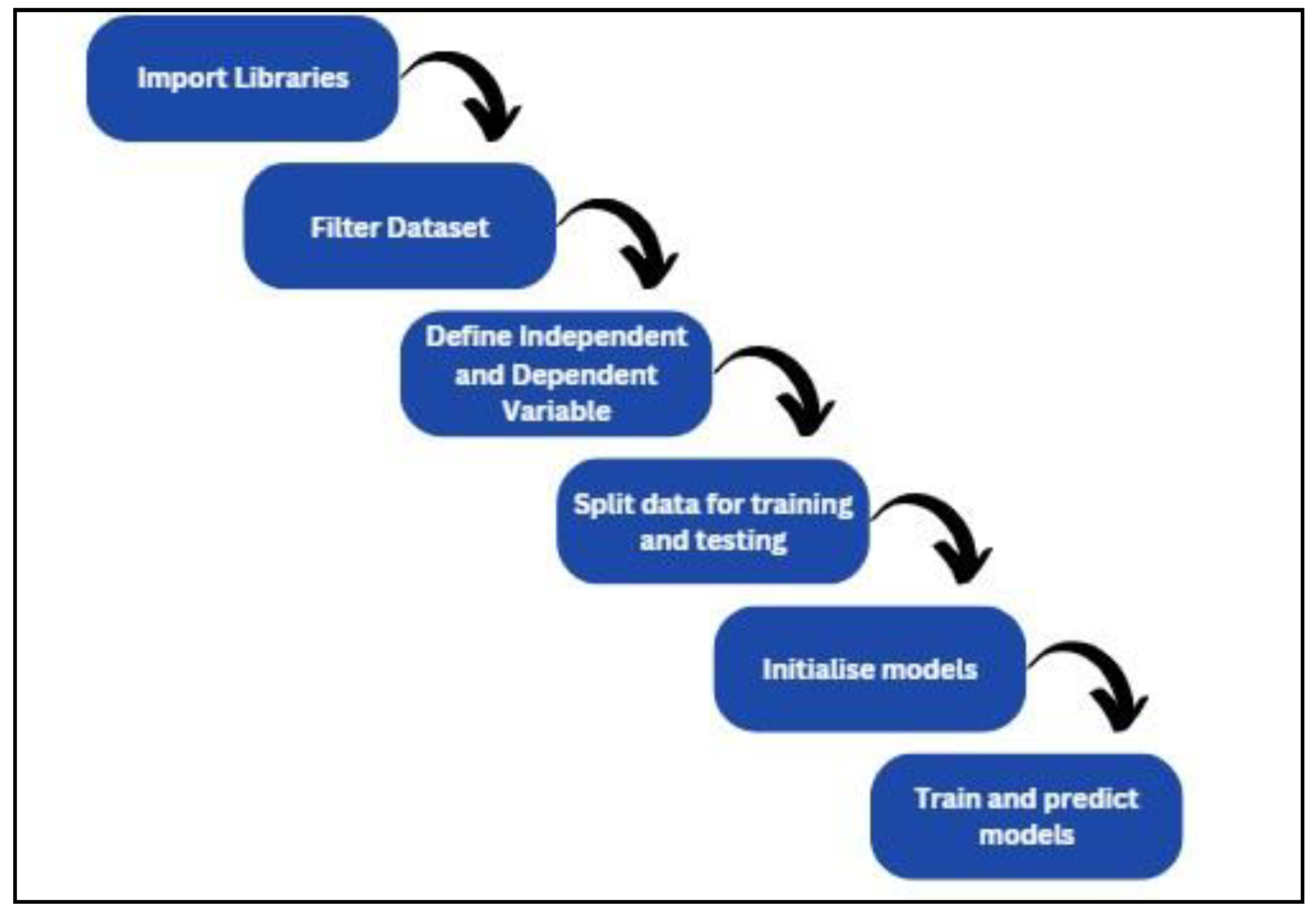
The machine learning flowchart demonstrates the steps that should be taken to create a machine learning model.

Figure 17. Machine Learning Flowchart.

Figure 17. Machine Learning Flowchart.

Next, the machine learning model libraries are called from ’sklearn’ like LinerRegression, RandomForestRegressor and GradientBoostingRegressor. The libraries from ’sklearn.model_selection’ also need to be imported to train, test and validate the model. Functions from ’sklearn.metrics’ can be employed to determine the performance of the model. Libraries like numpy, matplotlib.pyplot and seaborn are imported into the code to ease numerical operations, to plot validation results and enhance data visualisation. Following this, columns that will be used to train the model (X) and target variables (y) need to be initialized.Data is divided into train and test sets using the ’train_test_split’ function such that random 80% of data will be used for training and 20% of data will be used for testing. By providing a random state to feed, the random split of data is made reproducible, and thus the model can be replicated in the future.

Finally, the trained model constructed can be trained on the training data and use them for prediction in the test set. The predictions enable an evaluation of the accuracy of all the models, which assists in determining the best approach to predict the target variable.

4.5. Linear Regression

The code below uses various features to predict a target variable using Linear Regression. The code is divided into three parts, namely Training and prediction, providing coefficients, and testing that model.The output is highly informative regarding the model’s performance by displaying the coefficients of all features, the mean squared errors, and the R-squared value. Age, BMI, children, sex, smoking status, region, and other features have coefficients indicating their predictive importance for the target variable; the smoking variable has a high positive coefficient, indicating its importance to the goal value.

4.6. Random Forest Regression

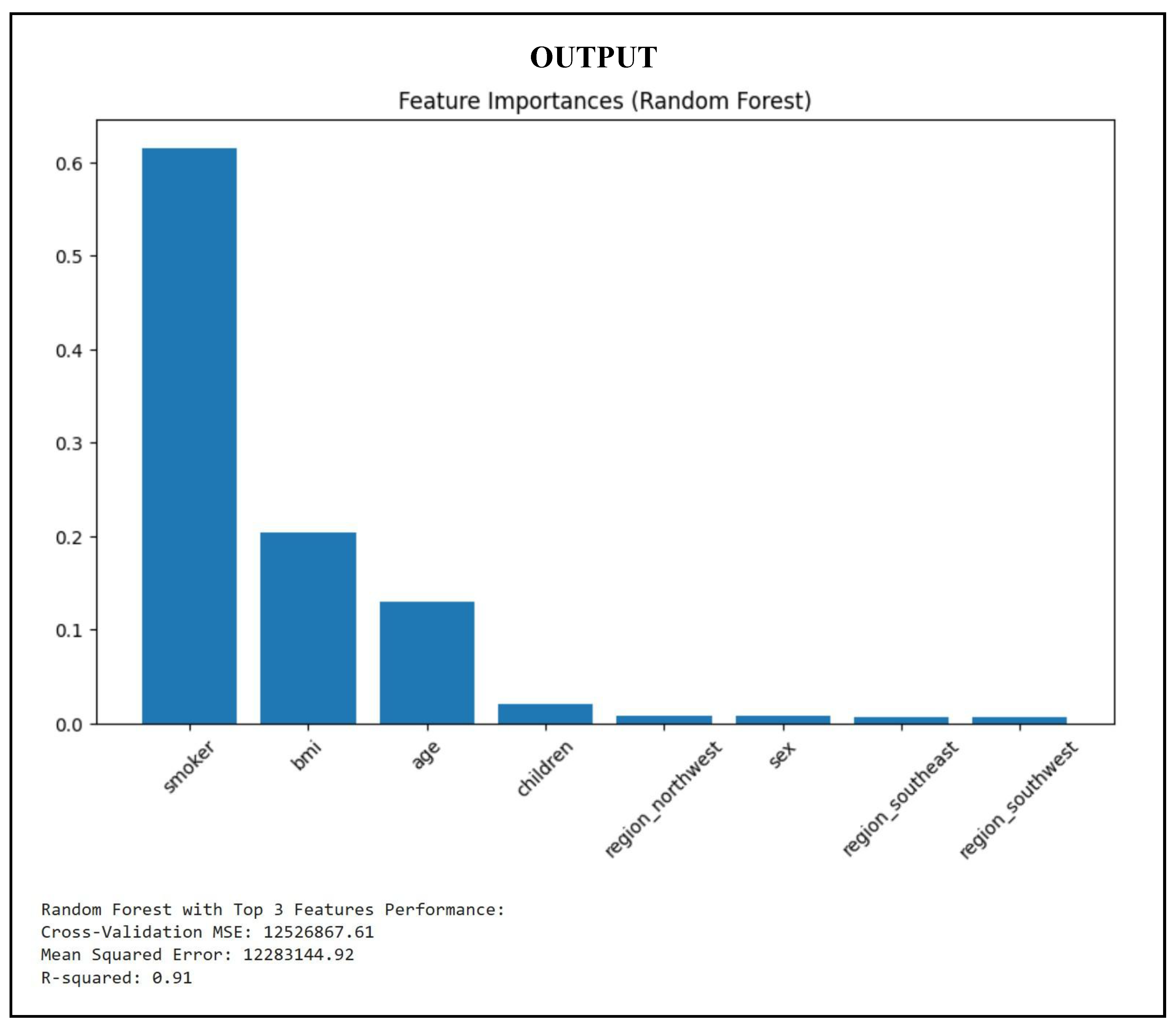
The following lines of code calculate the feature importance and model effectiveness in training and prediction phases of a dataset using Random Forest Regression. The code is used to construct a Random Forest Regressor, which fits into the training dataset and provides predictions for the test dataset. The code fetches the values of feature importance after training and plots them using a bar chart. The three primary features are again used to further split the data into new training and testing sets. The smaller dataset is used to recreate and train the Random Forest Regressor. Finally, the approach uses a 5-fold cross-validation with negative mean squared error as the metric to test the performance of the Random Forest model with selected features.

Figure 18. Train Random Forest Regression Model.

Figure 18. Train Random Forest Regression Model.

The results indicate that the smoker variable has the greatest effect on insurance pricing, followed by BMI and age. Concentrating on the three primary aspects enhances interpretability and efficiency, perhaps accelerating the model and increasing its clarity in production environments.

4.7. Gradient Boosting Regression

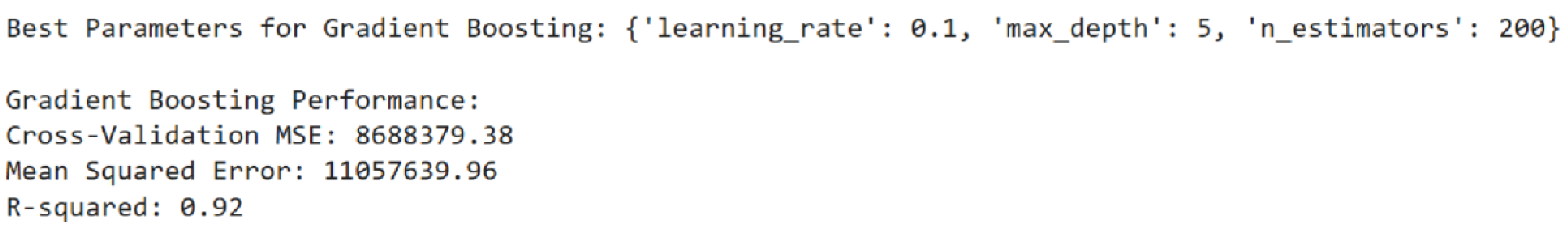
To optimise the Gradient Boosting Regressor, the code includes a ‘param_grid’ dictionary that specifies hyperparameters such as ‘n_estimators’, ‘learning_rate’, and ‘max_depth’. It uses 5-fold cross-validation using ‘GridSearchCV’ to identify the ideal parameter combination based on the negative mean squared error score metric. Metrics that evaluate the model’s generalisability, predictive accuracy, and R-squared Score include Cross-Validation MSE, MSE on the Test Set, and R-squared Score.

Figure 19. Train Gradient Boosting Regression Model.

With a learning rate of 0.1 and a maximum depth of 5, the Gradient Boosting model’s ideal parameters produced the lowest cross-validation error, suggesting strong generalisation. The model performs consistently across several data splits and shows minimal overfitting, as seen by the tight Cross-Validation and Test MSEs. 92% of the variation in the target variable can be explained by the model, which has an R-squared score of 0.92.

5.0. Model Validation

By showing the difference between the predictions and the actual values, this portion of the model validation process seeks to assess the machine learning models’ accuracy.

Figure 20. Model Validation.

Figure 20. Model Validation.

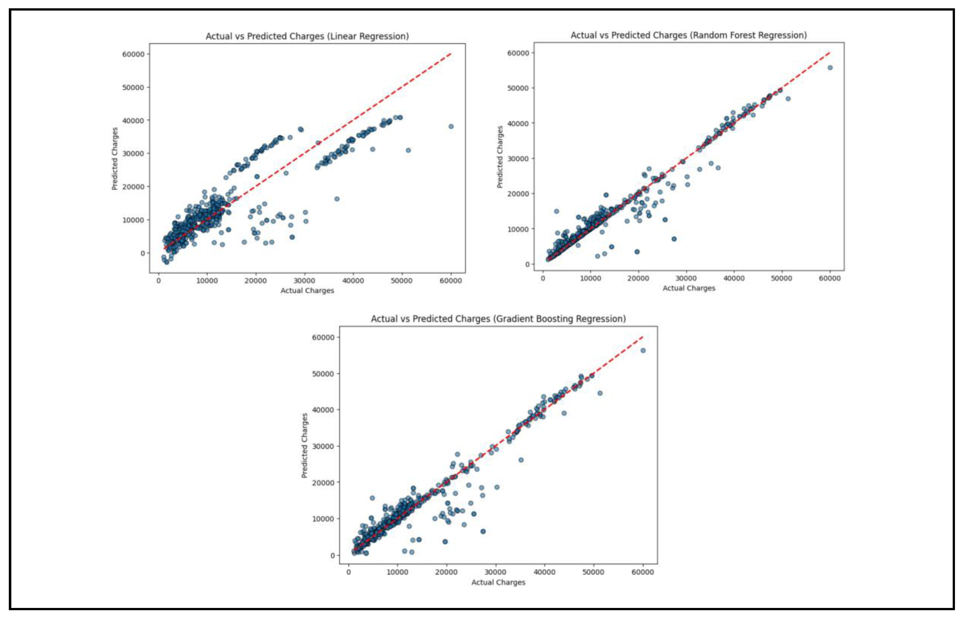
In order to visualize the differences between the actual and predicted costs of insurance, scatter plots are created using the plot_actual_vs_predicted function. The figsize command is used to provide the figure size as 8 inches by 6 inches using the figsize command. Finally, plt.scatter is used to make a scatter plot with y_test values (actual values) on the x-axis and y_pred values (predicted values) on the y-axis. To assist in visualizing comparing the actual and predicted values, an ideal prediction line is also graphed diagonally on the plot. To assist the scatter plot to be more readable, it is accordingly labeled. Subsequently, this function is used to graph the accuracy of each of the three machine learning models (Linear Regression, Random Forest Regression, and Gradient Boosting Regression).

Figure 21. Model Validation Output.

Figure 21. Model Validation Output.

6. Actual vs Predicted Changes (Linear Regression)

From this graph, many points are somewhat close to the line, signifying good performance for a linear regression model but with scatter happening especially at higher charge values. The close clump in the bottom left implies that the model has good forecast for low medical chargers. This means the model is more effective for the easy cases because medical charges are low and easy to forecast. For the higher charger, the predicted values are distant from the red line. There is systematic underprediction, particularly for charges above 40,000. In summary, this model is not highly accurate especially for higher medical chargers.

6.2. Predicted vs Actual Changes (Random Forest Regression)

In this graph, the majority of the predicted values are closely following the red line, which means that the model is good at predicting charges. There are some outliers that can be seen, meaning that some of the predictions are far away from the actual values. Generally, the Random Forest Regression model is accurate, as it has very few visible outliers.

6.3. Actual vs Predicted Changes (Gradient Boosting Regression)

Here, the points are all densely packed together along the red line, as is the Random Forest Regression graph. This is indicative of the fact that all of the estimates are quite good and close to actual values. Similar to Random Forest Regression, few apparent outliers are visible. Therefore, the Gradient Boosting regression model is accurate.

6.4. Learning Curve Evaluation

To create learning curves for machine learning models being utilized, there is a defined function named plot_learing_curve in this code. Learning curves are vital in assessing model performance since they give the size of accuracy of a model as well as pointing out overfitting or underfitting. The function uses four parameters and these are model, feature vector (x), target (y) and plot title. Lastly, the function learning_curve is called to calculate training and cross-validation scores. cv=5 instructs it to use five-fold cross-validation, and scoring=neg_mean_squared_error to calculate performance based on the negative mean squared error. By stating n_jobs=-1, the parallel computation gets activated, thus speeding up calculation. Lastly, the test and training scores get negated and transformed into positive mean squared errors. The cross-validation and training errors are plotted against the size of the training in a 10x6 sized plotted figure. Labels are introduced to enhance the visualisations and enable better understanding.

Learning curves for each of the three models—Linear Regression, Random Forest Regression, and Gradient Boosting Regression—are then generated with the function. To minimize dimensionality, Random Forest Regression generates its learning curve based on only the three most significant characteristics.

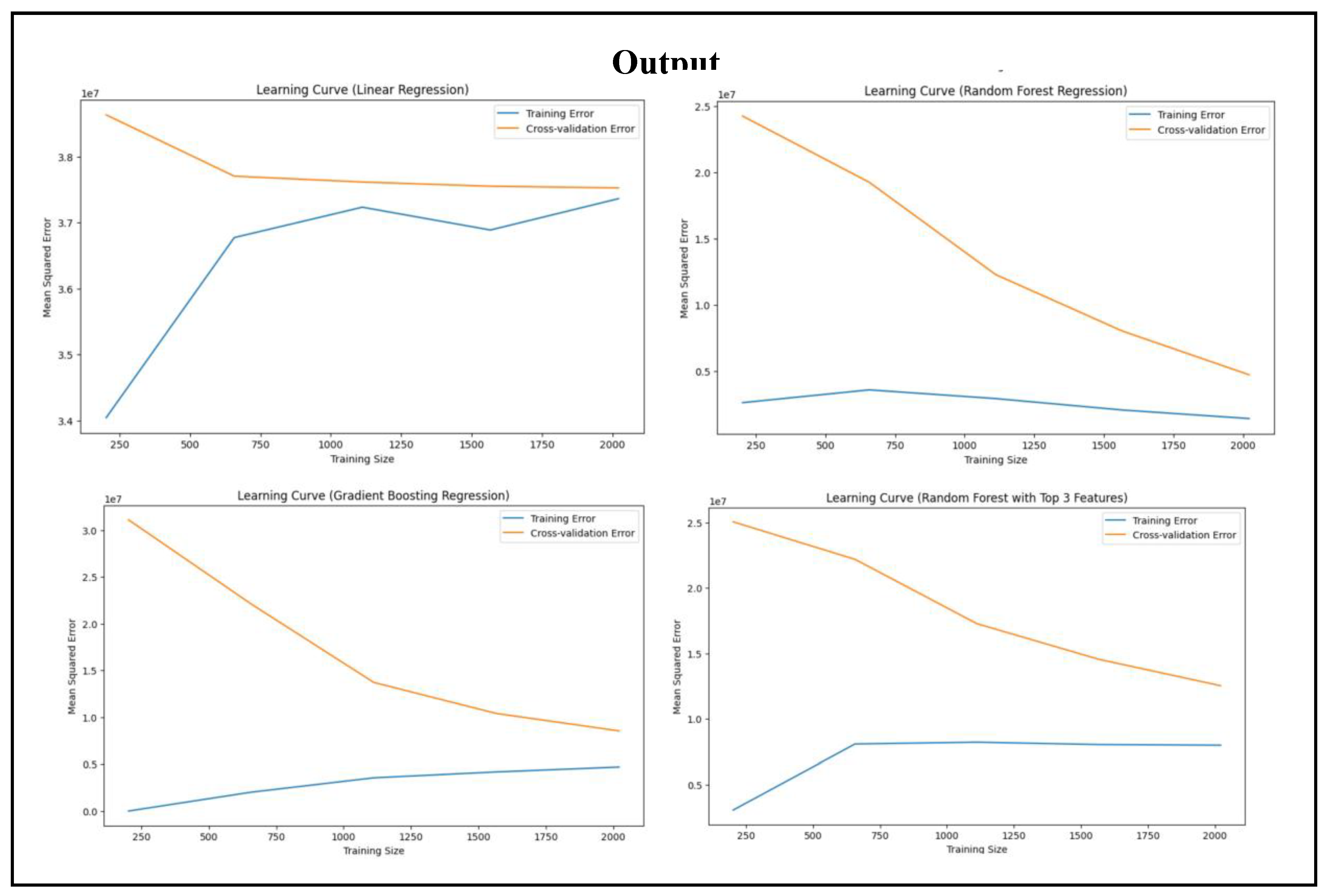
Figure 22. Learning Curve for Regression Models.

Figure 22. Learning Curve for Regression Models.

6.5. Learning Curve (Linear Regression)

The training error (blue line) starts low for small training size, but increases and becomes stable as the size grows. The cross-validation error (orange line) starts high due to insufficient training data, but decreases and becomes stable. This indicates that neither underfitting nor overfitting, but the stabilised error indicates that some bias exists.

6.6. Learning Curve (Random Forest Regression)

The training error (blue line) remains low throughout. This indicates that the model possesses great fit with the training data. The cross-validation error (orange line) starts high but decreases when the training set increases in size, which indicates greater generalisation. The distance between the two lines narrows down, which means better model performance with more data.

6.7. Learning Curve (Gradient Boosting Regression)

The training error (blue line) does not increase much with the size of training, which indicates less overfitting. The cross-validation (orange line) decreases considerably as the training size is larger, which indicates improved generalisation. The lines converge, which indicates that overfitting is reduced and this model works better with more data.

6.8. Learning Curve (Random Forest with Top 3 Features)

The training error (blue line) is low and flat across, meaning the training set can adapt satisfactorily to this model. The cross-validation error (orange line) decreases consistently as more data is used. There is also space between the two lines, showing that there is some amount of overfitting.

6.9. Conclusions from Regression Models

From this study, the most powerful predictor of insurance rates was smoking, with a very high correlation with rates. BMI was also positively correlated with rates, showing that higher-BMI individuals have somewhat higher medical costs. Age, however, was a less consistent predictor, with less impact than smoking and BMI. Gender and geographic differences were unrelated to charges, as one would expect from the dataset structure. Linear Regression could not detect non-linear interaction, while Random Forest Regression was able to select useful features but experience a little overfitting in the learning curve. Gradient Boosting Regression achieved the greatest R-squared value and least overfitting, as expected from its excellent performance in detecting complex relationships.

7.0. Conclusions

Machine learning can be an excellent tool to help with identifying, evaluating and aiding decision-making for significant decisions to help develop solutions to significant problems. But there is definitely a need to make the machine learning software trustworthy to everyone, with great precision and accuracy, to aid individuals in real-world applications. For example, to give low-cost medical bills and relieve the healthcare burden on individuals who lack the monetary capacity of maintaining their own health. Machine learning can spot problems more quickly than human beings, and hence is vital to guarantee the pace to produce quicker but effective solutions to problems in question.

The project used regression algorithms to forecast health expenditures and attributed smoking as the primary cause. Lifestyle factors such as BMI and age also affected healthcare expenditures. Gradient Boosting Regression showed higher accuracy with very little overfitting, whereas Random Forest Regression offered feedback regarding feature importance. Linear Regression is hampered by its inability to identify non-linear patterns, particularly where there are large expenditures.

By using machine learning algorithms, the model can learn and could derive plausible conclusions and results with hardly any human input, and while it’s useful to most disciplines, attempts have to be made to keep such models extremely computationally efficient and precise, and hence conditions like overfitting, underfitting, and dimensionality is best avoided for maximum performance. After all, people desire the best result from the best performance of a machine learning model that can be considered a model for ensuring the best solutions to be presented for real-world situations and phenomena.