Submitted:
22 February 2025
Posted:
24 February 2025
You are already at the latest version
Abstract
Accurate inflation forecasting is crucial for effective monetary policy, particularly during turning points that demand policy realignment. This study examines the efficacy of Shallow Neural Network Ensemble Models in predicting U.S. inflation turning points more precisely than traditional methods, including the Survey of Professional Forecasters (SPF). We employ monthly data from January 1970 to May 2024, training these ensemble models on information through December 2022 and testing on out-of-sample observations from January 2023 to May 2024. The models generate forecasts at horizons of up to 16 months, accounting for both short- and medium-term dynamics. Results indicate that Shallow Neural Network Ensemble Models consistently outperform conventional approaches using key performance metrics, notably detecting inflation turning points earlier and projecting a return to target levels by May 2024 - several months ahead of the Survey of Professional Forecasters’ average forecast. These findings underscore the value of such ensembles in capturing complex nonlinear relationships within macroeconomic data, offering a more robust alternative to standard econometric methods. By delivering timely and accurate forecasts, Shallow Neural Network Ensemble Models hold great promise for informing proactive policy measures and guiding decisions under uncertain economic conditions.
Keywords:
Inflation forecasting
; Shallow neural network ensembles
; Nonlinear modeling
; Machine learning
; Out-of-sample prediction
; Survey of Professional Forecasters
1. Introduction
Accurate inflation forecasting is pivotal for effective monetary policymaking, particularly when a shift in policy stance is warranted to determine turning points in the economy. In this study, we compare the performance of Shallow Neural Network Ensemble Models with the Federal Reserve Bank of Philadelphia’s Survey of Professional Forecasters (SPF) average forecast, focusing on whether or not these ensemble methods provide enhanced predictive accuracy for U.S. inflation. Our findings indicate that these ensemble models are significantly more accurate than the SPF and also identify a break in trend inflation several months ahead of the SPF. Demonstrating improvements relative to the SPF’s widely followed benchmark thus underscores a meaningful contribution to current forecasting practices.[1]
Historically, a robust literature supports the importance of better forecasting in economics and management science, especially under conditions of financial volatility (Dia 2001; Binner et al. 2004a,b; Tsay, R. S. 2005, Zhang and Qi, 2005; Bodyanskiy and Popov 2006; Curry 2007; Cao 2012, Binner et al. 2024. A long-held macroeconomic hypothesis posits that a stable relationship exists between the growth rate of the money supply and the growth rate of prices (Friedman and Schwartz 1970; Barnett 1997; Nelson 2003). Conventional econometric methods have scrutinized this linkage extensively, yet evidence of nonlinear effects and structural breaks (Bachmeier et al. 2007) has led to an exploration of artificial neural networks (ANN) as an alternative (Virili and Freisleben 2000; Giles et al. 2001). Such methods potentially avoid pitfalls associated with cointegration tests in the presence of evolving payment technologies or nonstationary conditions (McCallum 1993).
Traditional statistical models of time-series forecasting enjoyed considerable success from the 1950s onwards, beginning with exponential smoothing (Brown 1956; Holt 1957) and progressing to the Auto-Regressive Moving Average (ARMA) model (Whittle 1951). Box and Jenkins (1970) extended ARMA to ARIMA(p,d,q), addressing nonstationarity by incorporating a differencing parameter, (d), and later introduced seasonal adjustments (SARIMA) to account for seasonality. These innovations brought systematicity and reproducibility to time-series forecasting, and many practitioners subsequently migrated from univariate approaches to multivariate variants such as ARIMAX and SARIMAX, which incorporate exogenous variables. Further advancements allowed multiple input-output relationships in Vector AutoRegressive (VAR), Vector Moving Average (VMA), and Vector AutoRegressive Moving Average (VARMA) models (Sims 1980). Indeed, ARIMA and VAR models have demonstrated success in macroeconomic forecasting (Stock and Watson 2007; Ruslan et al. 2018). However, a thorough comparison of these linear techniques with complex machine learning methods by Makradakis et al. (2018) and Makridakis and Hibon (2000) revealed that simple linear models often outperformed nonlinear models in small-sample settings. Later work by Cerqueira et al. (2019) showed that machine learning methods may indeed surpass linear benchmarks as sample sizes grow, potentially overcoming the tendency to overfit. More recently, Orojo et al. (2023) found that a multi-recurrent neural network (MRN) could outperform traditional methods when dealing with more complex time-series data.
Despite their effectiveness, linear models such as ARIMAX, SARIMAX, and VAR face several challenges, including assumptions of linearity, stationarity, and stable structural relationships (Petrica et al. 2016). Nonlinear methods, by contrast, can capture dynamic patterns arising from disruptive technological changes or macroeconomic shocks (Kelly et al. 2024; Narayanaa et al. 2023; Nakamura 2005; Chen 2020). Markov switching or regime switching models address some nonlinearities by allowing parameters to vary across regimes (Goldfeld and Quandt 1973; Hamilton 1988, 1989, 1994), but they rely on predefined transition probabilities and stationary Markov chains, which can limit flexibility (Briggs and Sculpher 1998). Recurrent neural networks (RNNs), including Long Short-Term Memory (LSTM) and Gated Recurrent Units (GRU), may sidestep some of these constraints by offering continuous, dynamic memory across regimes (Hochreiter and Schmidhuber 1997; Lin et al. 1996; Tepper et al. 2016). However, RNNs can be computationally intensive (Bengio 1994) and have historically struggled with vanishing gradients, prompting research into architectures featuring memory cells and gating mechanisms (Cho et al. 2014).
In recent years, attention has shifted towards more complex network architectures such as Transformers (Vaswani et al. 2017), which leverage attention mechanisms, and excel at handling large-scale data in parallel (Roumeliotis et al. 2023). Surprisingly, several studies suggest that Transformers may not consistently outperform simpler RNN variants in time-series forecasting (Murry et al. 2022; Zeng et al. 2022). Moreover, shallow feedforward neural networks remain appealing due to their relative simplicity and generally robust function approximation capabilities (Rumelhart et al. 1986; Goodfellow et al. 2016).
Against this background, we investigate whether an enhanced RNN—a member of the simple recurrent network class that incorporates a temporally sensitive memory mechanism, can more accurately forecast inflation turning points than conventional approaches, including the SPF’s average forecast. We use U.S. data spanning January 1970 to May 2024, training and validating our model from January 1970 to December 2022, and then generating out-of-sample forecasts for January 2023 to May 2024. The RNN model produces step-ahead forecasts from t+1 to t+16, enabling an assessment of both short-term and medium-term inflation dynamics. By examining whether critical predictive signals embedded in historical data can improve turning-point detection, our research aims to offer new insights into the utility of machine learning—specifically Shallow Neural Network Ensemble Models, for guiding monetary policy decisions. Our principal conclusion is that these ensemble methods provide a robust alternative to more traditional econometric and survey-based forecasts, thereby contributing to the ongoing debate on how best to capture the complexities of modern macroeconomic data.
2. Materials and Methods
2.1. Data
We begin with an overview of the data. Figure 1 shows the month over month percentage change and level of the U.S. consumer price index (CPI), the month over month percentage change in U.S. monetary aggregate, Divisia M4 (DM4) and Divisia M2 (DM2), as well as the 3-month T-Bill Rate. Divisia M4 is a broad money measure published by the Center for Financial Stability, CFS, New York (See Belongia and Binner, 2000, for details on the construction and interpretation of evidence on the macroeconomic performance of Divisia monetary aggregates for eleven countries). Divisia M2 use applies the same Divsia monetary aggregation method to monetary assets include in the US Federal Reserve’s M2 definition.
2.2. The Multi-Recurrent Network Methodology
Machine learning techniques are concerned with general pattern recognition or the construction of universal function approximators, Cybenko (1989), that can detect relationships in the data in situations where no obvious patterns exist. The power of neural network approximations is summarized in the well-known theorem of Hornik et al. (1989), which essentially states that a neural network can approximate all probability density functions supported compactly on the real numbers. In view of Dorsey’s (Dorsey 2000, pp. 30–31) contention that standard econometric methods have provided no concrete evidence one way or the other to explain the link between money growth and inflation, we believe neural networks offer more promise in the context of econometric modeling than standard linear models. In essence, this approach helps to define the parameter space in a framework akin to a regime-switching model where the regimes themselves are nonlinear relationships. Although this is somewhat unusual in this context, the application of neural networks in economics and finance is growing, as indicated by the wide range of studies surveyed in Binner et al. (2004a, b, 2005, 2010, 2018, 2025, forthcoming).
A key limitation of the traditional neural network models used for inflation forecasting by Gazely and Binner (2000), Dorsey (2000), and Binner et al. (2005) is that they rely on the feed-forward multilayered perceptron (FF-MLP) trained with standard backpropagation (Rumelhart et al. 1986). Although the limitations of the backpropagation algorithm are well-known, it is the feed-forward nature of the architecture that restricts the types and robustness of temporal dependencies these models can learn and represent. Typically, historical input information must be provided as a temporal input window, which is pre-determined (e.g., a six-month window requiring six months of past values for each explanatory variable). Determining the optimum window size must be done empirically, and the strictly forward flow of information confines these models to acting as non-linear auto-regressive (NLAR) models. Should a moving average component or previous output behavior be essential for the learning task, more complex architectures are required that introduce feedback connections.
Building on our previous successes (Kelly et al. 2024; Tepper et al. 2016; Orojo et al. 2019, 2023), we use a state–of-the-art multi-recurrent network (MRN) in this paper. The Back-propagation learning rule (Rumelhart et al. 1986) and its variants are used to train these neural networks (including the MRN) and is considered a powerful optimization technique enabling sophisticated curve fitting (Refenes and Azema-Barac 1994). A main tenet of backpropagation is its aim to minimize the difference between the network’s predicted output and the actual target output, akin to finding a function that best fits a set of data points.
The curve-fitting ability of an MRN is directly influenced by hyperparameters such as the number of hidden layers and the number of neurons in each layer, analogous to choosing the order of a polynomial. An insufficiently complex model leads to poor fit and prediction, whereas an overly complex model risks overfitting and weak generalization. Neural networks are inductive, meaning they can learn from empirical regularities even when the precise governing rules of a phenomenon are not known. This property is advantageous in economic contexts, where the goal is often to model highly complex systems while retaining predictive power. The learning process allows the network, in effect, to disregard excess input variables. Hence our methodology requires a large amount of rigor in terms of the machine learning model fitting and selection process.
Our methodology aligns with the curve-fitting perspective outlined by Refenes and Azema-Barac (1994) rather than with traditional statistical approaches, such as those used by Cont (2001) in examining various statistical properties of asset returns. Cont’s (2001) work deals more with distributional properties, tail dynamics, and nonlinear dependence over time. Traditional back testing, commonly applied in statistical models for financial market trading, can obscure overfitting when used with recurrent neural networks (Shirdel et al. 2021). As a result, the orthodox approach to mitigating overfitting in models like the MRN involves regularization (to diminish the impact of unimportant features) and ensembling (combining predictions from multiple machine learning models). These advantages will be further considered when discussing the MRN’s architecture and forecasting methodology in the following section. We follow a robust model fitting and selection methodology consistent with Orojo et al (2023) and also introduce an ensemble-based technique to minimize variance, in conjunction with L2 regularization, as stated above.
This class of RNN extends the traditional FF-MLP architecture to include recurrent connections that allow network activations to feedback as inputs to units within the same or preceding layer(s). Such internal memories enable the RNN to construct dynamic internal representations of temporal order and dependencies which may exist within the data. Units that receive feedback values are often referred to as context or state units. Also, assuming non-linear activation functions are used, the universal function approximation properties of FF-MLPs naturally extends to RNNs. These properties have led to wide appeal of RNNs for modelling economic time-series data, Ulbricht (1994); Moshiri, et al. (1999); Tenti (1996); Tino et al (2001); Binner et al. (2004a, b); Binner et al (2010), Cao et al (2012) and Tepper et al. (2016).
The MRN architecture is shown in Figure 1 and can be expressed generally as:
where denotes the predicted month-on-month percentage change in inflation for a particular forecast horizon, , where we explore horizons τ=1 to 16. As described in Section 2 and later in this Section, the external input vector x consists of between two to five input variables representing combinations of: the previous month-on-month percentage change in inflation, natural log of the price level, 3-month treasury bill secondary market rate, and month-on-month growth rates (%) for DM2 or DM4.
c (the context vector) forms a complex internal memory state vector that is the concatenation of the: previous hidden state vector (h; previous output vector ( and the previous external input vector, (x. We extend each allowable feedback by additional banks of context units (memory banks) on the input layer. The number of additional memory banks relates directly to the degree of granularity at which past and current information is integrated and stored and enables the network to implement a form of sluggish state-based memory to inform decision making over variable-width time delays. Following Ulbricht (1994), Binner et al (2010), Tepper et al (2016) and Orojo et al (2023), we use memory banks where as experience has shown that moving beyond this does not lead to enhanced performance for the problems addressed. c represents an internal memory of varying rigidity; that is some context units will represent information from very recent time steps and thus change rapidly whilst others will represent information further back in time and change much more slowly. To achieve this, the unit values fed back from the hidden and output layers are combined, to varying degrees, with their respective context units, , in the input layer, as determined by the weighting values applied to its recurrent links. The influence of the previous context unit values is determined by the weighting values applied to the self-recurrent links. When the weighting on the recurrent links is greater than those on the self-recurrent links then more flexible memories are formed storing more recent information at the expense of historical information stored in the context units. Conversely, if the weighting values on the self-recurrent links are greater than those on the layer recurrent links then more rigid memories are formed since more historical information is preserved in the context units at the expense of the more recent information being fed back from subsequent layers. It is these layer- and self-recurrent link ratios that collectively implement a sluggish state memory whereby network outputs (or decisions) are based on variable integrations of recent and distant past unit activations from the input, hidden and output layers. This weighted integration of current and past information can be generally expressed as follows:
where , refers to context unit i at time t; denotes either an output activation, hidden unit activation or external input value at time t-1; refers to the connection strength of the recurrent link from to where where ; refers to context unit i at time t-1; and finally refers to the connection strength of the self-recurrent link for where . x is the external vector of input variables.
is the weight matrix connecting the external input vector to the hidden layer; is the weight matrix connecting the context vector to the hidden layer; is the weight matrix between a single constant input unit, equal to 1, and the hidden layer (representing the hidden threshold or bias term); is the weight matrix connecting the hidden layer to the output layer and is the weight matrix between a single constant unit, equal to 1, and the output layer, again representing the output threshold or bias term. The vector function, f, and function g return the activation vectors from the hidden and output layers, respectively. We apply the hyperbolic tangent function, , to the inner products performed for f to compute the hidden unit values as shown below for a single hidden unit, :
Where The number of hidden units is a significant hyper-parameter for this model and is empirical. Finally, we apply the identity function, , for the inner products performed for g to compute the output unit values as shown below for a single output unit, :
Where We use back propagation-through-time (BPTT), (Werbos, 1990; Williams and Peng, 1990), to minimize the following mean-squared-error (MSE) measure:
where , refers to the number of input patterns and , the number of output units. BPTT is an efficient gradient-descent learning algorithm for training RNNs where weight changes are determined by a sequence, or time-lag, of input observations rather than a single observation. Input data were scaled to zero mean, and unit variance. To facilitate convergent learning, a linearly decaying learning rate and momentum schedule are used for all training experiments with an initial learning rate of 0.0001 and momentum term of 0.95. This provides an effective time varying learning rate that guarantees convergence of stochastic approximation algorithms and has proven effective for temporal domains, for example, see Lawrence et al. (2000). To minimize the onset of over-fitting, in addition to the ensemble-based methodology discussed later, we apply L2 weight regularization during training with the lambda constant set at 0.001. We generate independent training sequences directly from the time-series using a time window whose lag size is empirically established, i.e. 120 months for the US inflation problem tackled here. The MRN context units are initialized to known values at the beginning of each sequence of data and each element within a sequence is processed sequentially by the network. Although this restricts the MRN to behave as a finite memory model and means that the MRN must first learn to ignore the first context values of each sequence, it allows for efficient randomized learning.
Although such RNNs and variants thereof have enjoyed some success for the time-series problem domains, we tread with cautious optimism. Due to the additional recurrency, such models inherently contain large degrees of freedom (weights) which may require many training cases to constrain. Also, gradient descent-based learning algorithms are notoriously difficult at finding the optimum solution the architecture is theoretically capable of representing: Bengio et al. (1994) and Sharkey, et al. (2000). However, the embedded memory architecture within the MRN may compensate for this deficiency, as demonstrated recently by Tepper et al. (2016) and more recently by Orojo et al (2023). For a comprehensive account of the strengths and limitations of both feedforward and recurrent neural networks and how to optimize them, please see the classic textbook by Goodfellow et al (2016).
Based on the feature set used, we construct the following three types of MRN:
- a)
- simple MRN consisting of three input variables: the month-on-month percentage change in inflation (cpi_percmom, the auto-regressive term), the natural log of the price level (ln_cpi_level) and 3-Month Treasury Bill Secondary Market Rate (dtb3).
- b)
- intermediate MRN which includes a) plus the month-on-month growth rate (%) for the Divisia monetary measure DM4 (dm4_percmom).
- c)
- complex MRN which includes b) plus the month-on-month growth rate (%) for the Divisia monetary measure DM2 (dm2_percmom).
For each of the above feature sets, we follow the same approach used by Binner et al (2024b) and develop a set of sixteen MRN ensembles where each MRN has a monthly input lag structure spanning 10 years and a single hidden layer with 50 non-linear units is assigned to predict a particular forecast horizon of the month-on-month percentage change in inflation, i.e. t+1, t+2,…, or t+16. Each ensemble consists of five independently trained MRNs fitted to the in-sample period of January 1970 – December 2022 and then evaluated on the out-sample period of January 2023 to April 2024; thus a total of 80 MRNs were generated for each of the three feature sets. As mentioned earlier, a series of independent training sequences of 120 months are generated directly from the time-series and presented in a random fashion to each MRN during the training process, where the context units are initialized to some known value at the beginning of each sequence, and the forecast generated in response to the last observation in the training sequence being stored as the prediction for that particular sequence.
The out-of-sample forecast for each trained MRN is generated in response to being sequentially fed the first out-of-sample input window containing observations from January 2013 until December 2022. The MRNs trained to predict t+1 are responsible for the January 2023 forecast, the models trained to predict t+6 are responsible for June 2023 forecast and so on. Each prediction is an average of the respective five MRNs associated with the dedicated forecast horizon. During the out-of-sample period, no further parameter estimates are obviously allowed. As the sequential input window slides over time, only new input observations are passed through the network as they become available. This forecasting methodology is depicted in Figure 3 below. In terms of backtesting, given our previous research exploring different configurations of training, validation and test samples, we have adopted a more efficient approach to the problem of identifying the appropriate level of model complexity by applying regularization and ensemble-based aggregation. We then apply our fitted models to the unseen out-of-sample data.
This is analogous to an SPF making long term forecasts at the end of December 2022 based only on rules they have derived from studying observations between January 1970 and December 2022.
2.3. Survey of Professional Forecasters (SPF)
The purpose of this study is to contrast the performance of macroeconomic forecasts using artificial neural networks to those made by the methods using human judgement that we represent by the Survey of Professional Forecasters (SPF). The SPF is the oldest quarterly survey of macroeconomic forecasts in the United States. The survey began in 1968 and was conducted by the American Statistical Association and the National Bureau of Economic Research. The Federal Reserve Bank of Philadelphia took over the survey in 1990. The Survey of Professional Forecasters' is a statistical survey, and the official web page offers the actual releases, documentation, mean and median forecasts of all the respondents as well as the individual responses from each economist; the latter are kept confidential with the use of identification numbers, please see https://www.philadelphiafed.org/surveys-and-data/real-time-data-research/survey-of-professional-forecasters). It compiles predictions from a diverse panel of professional economists on key economic indicators, including inflation, real GDP, and unemployment. Specifically, the SPF’s inflation forecasts draw widespread attention from policymakers and market participants, serving as a central benchmark for comparing different predictive methods. Because it aggregates forecasts from experts in academia, industry, and financial institutions, the SPF provides a consensus view of future inflation trends over various time horizons. Data from the SPF are publicly available and are regularly updated, allowing researchers and practitioners to assess forecast accuracy, detect shifts in economic sentiment, and evaluate new forecasting models against a longstanding, reputable standard.
2.3. Forecast Evaluation Procedure
Each of the neural network models is compared to the Survey of Professional Forecasters’ (SPF) average inflation forecast over the simulated out-of-sample period from January 2023 through December 2023, providing robust evidence for or against meaningful improvements in forecasting accuracy. To facilitate this comparison, we employ three primary forecast evaluation metrics:
- Root Mean Squared Error (RMSE), which measures average forecast errors and emphasizes large deviations.
- Symmetric Mean Absolute Percentage Error (sMAPE) which expresses errors as a percentage, simplifying comparisons across different scales.
- Theil’s U Statistic, which compares model performance to a naïve forecast, with lower values indicating better accuracy.
- Improvement Over Random Walk, which quantifies how much better a forecasting model performs compared to a random walk benchmark, expressed as a proportion
3. Results
3.1. Forecast Evaluation
Table 1 compares five forecasting methods, i.e., simple MRN, intermediate MRN, complex MRN, average MRN, and SPF, across these evaluation metrics. The average MRN method demonstrates the lowest RMSE and sMAPE, signifying the smallest average forecast errors. It also achieves the lowest Theil’s U (0.104), which suggests that it closely aligns with actual values and performs significantly better than a random walk. The high Improvement score of 0.896 for average MRN reflects an almost 90% reduction in forecast error over the baseline, indicating a substantial predictive advantage.
The simple MRN model also performs well, with an Improvement score of 0.876 and a Theil’s U of 0.124, suggesting it is nearly as accurate as average MRN. Meanwhile, the intermediate MRN and complex MRN exhibit slightly higher error metrics and Theil’s U values, indicating that these models are somewhat less accurate. The SPF model, while showing moderate performance, has a relatively higher Theil’s U of 0.152, suggesting its forecast accuracy is less favorable compared to the average MRN and simple MRN. Overall, the average MRN is the best-performing model in terms of accuracy and predictive value, with simple MRN following closely behind. These models demonstrate a significant improvement over the random walk, making them reliable choices for forecasting applications.
3.2. Comparison of CPI and Forecasts Over Time
Figure 4 illustrates each forecasting model’s projection against the observed inflation rate over the test period. Notably, the MRN-based forecasts all suggest that inflation will return to near target levels by May 2024, in contrast to the Survey of Professional Forecasters (SPF), which predicts a near target-level return in October 2024. This discrepancy holds significant policy implications, as the Federal Reserve has faced criticism for delaying cuts to key policy rates.
4. Discussion
The comparative results presented here suggest that Shallow Neural Network Ensemble Models, or MRNs in some analyses, can offer notable improvements over conventional forecasts, such as those provided by the Survey of Professional Forecasters (SPF). Specifically, these models consistently project a return to near-target inflation several months earlier than the SPF, underscoring the potential value of machine learning approaches for capturing dynamic, nonlinear relationships in macroeconomic data. These findings align with previous studies that highlight the limitations of linear econometric models, e.g., ARIMA, VAR, when confronted with structural shifts or unanticipated shocks, please see Cerqueira et al. (2019) and Orojo et al. (2023) and more recently, Kelly et al (2025) using UK inflation data. By incorporating advanced memory mechanisms and ensemble averaging, the neural network models appear better equipped to interpret the historical trajectory of inflation, including subtle turning-point signals that might otherwise be missed by simpler or purely judgmental methods.
From a policy perspective, the difference in forecasting timelines could significantly shape decisions regarding interest rates and monetary policy interventions. As reflected in the discussion by Kristin Forbes (2023), adopting a faster or more aggressive tightening strategy may yield less labor market pain and a swifter re-anchoring of inflation expectations, whereas a more gradual approach reduces the risk of abrupt policy overcorrection. Evidence presented here that neural network models can detect turning points earlier than simpler models suggests that real-time deployment of machine learning forecasts may provide central banks with a more proactive warning system for emerging inflationary pressures or impending economic slowdowns.
In the broader context, these results reinforce growing evidence that data-driven, nonlinear modeling approaches can capture complex economic dynamics that traditional frameworks occasionally overlook. Future research might explore how these models fare in international settings or with higher-frequency data, such as weekly or daily price indices. Moreover, extensions could incorporate additional macro-financial variables—like commodity prices, credit conditions, or labor market indicators—to assess how enriched data inputs influence predictive accuracy. Finally, while our study focuses on inflation forecasts, similar ensemble neural network techniques could usefully be applied to other critical macroeconomic indicators, thus expanding their utility in both research and policymaking domains.
5. Conclusions
This study underscores the promise of multi-recurrent networks (MRNs) as a powerful tool for inflation forecasting, especially during pivotal turning points that demand policy intervention. By training and validating MRNs on historical data from January 1970 to December 2022, then testing out-of-sample performance from January 2023 to May 2024, we demonstrate that these models can predict inflation dynamics with greater precision than conventional methods such as the Survey of Professional Forecasters (SPF). Crucially, the average MRN model outperforms both traditional econometric approaches and simpler neural network variants across multiple metrics, including RMSE, sMAPE, and Theil’s U, providing earlier detection of shifts requiring policy adjustments.
Beyond their superior predictive accuracy, MRNs capture nonlinear and time-varying relationships that are often missed by linear frameworks. By leveraging advanced memory mechanisms, these networks offer actionable insights into inflationary trends well before conventional benchmarks, a finding of key relevance to central banks that require reliable forecasts up to 24 months in advance. As Croushore and Stark (2019) note, surpassing the SPF forecasts is considered a significant breakthrough in economic prediction, and the evidence presented here suggests that MRNs can do so consistently.
The importance of these results lies in their ability to guide timely and effective policy responses. Central banks frequently operate under conditions of substantial uncertainty, and the ability to detect turning points earlier can help them introduce measured interventions that reduce the risk of entrenched inflation or destabilizing economic shocks. Given the growing availability of granular, high-frequency data, MRNs’ aptitude for modeling complex dependencies places them at the forefront of a potential paradigm shift—one in which machine learning complements or even supersedes traditional econometric tools.
Future research will further refine MRNs by incorporating additional macroeconomic and financial variables, as well as by exploring ensemble or hybrid methodologies that extend the existing architecture to boost accuracy, robustness and generalizability. For example, experimenting with pruning deliberately over specified MRNs to find the optimum architecture for the problem, as demonstrated by Orojo (2022). Extending these methods to various economic contexts and time horizons would also illuminate the range of scenarios in which MRNs excel. This work has not addressed the welfare costs of inflation and we have assumed no menu costs as this topic is beyond the scope of this work but could fruitfully be incorporated into a future study, building on e.g. Hellwig (2008). Ultimately, the insights gleaned from MRNs can foster more responsive, data-driven policy decision-making, underscoring their growing importance in the economics and management science toolkit.
References
- Aydin, A., & Cavdar, S. (2015). Two Different Points of View through Artificial Intelligence and Vector Autoregressive Models for Ex Post and Ex Ante Forecasting. Computational Intelligence and Neuroscience, 2015, Article ID 714512. [CrossRef]
- Bachmeier, L., Leelahanon, S., & Li, Q. (2007). Money Growth and Inflation in the United States. Macroeconomic Dynamics, 11, 113–127. [CrossRef]
- Bank of England (2024). Bank of England Research Agenda for Research (2025 – 2028). Available online: https://www.bankofengland.co.uk/research/bank-of-england-agenda-for-research (accessed on 13th January 2025).
- Barnett, W.A. (1997). Which Road Leads to Stable Money? Economic Journal, 107, 1171–1185.
- Belongia, M.T., & Binner, J.M. (Eds.) (2000). Divisia Monetary Aggregates: Theory and Practice. Palgrave Macmillan. ISBN: 0-333-64744-0.
- Bengio, Y., Simard, P., & Frasconi, P. (1994). Learning Long-Term Dependencies with Gradient Descent is Difficult. IEEE Transactions on Neural Networks, 5(2), 157–166. [CrossRef]
- Binner, J.M., Gazely, A.M., Chen, S.H., & Chie, B.T. (2004a). Financial Innovation and Divisia Money in Taiwan: Comparative Evidence from Neural Network and Vector Error-Correction Forecasting Models. Contemporary Economic Policy, 22(2), 213–224. [CrossRef]
- Binner, J.M., Kendall, G., & Chen, S.H. (2004b). Applications of Artificial Intelligence in Economics and Finance. In T.B. Fomby & R.C. Hill (Eds.), Advances in Econometrics (Vol. 19, pp. 127–144). Emerald Publishing.
- Binner, J.M., Bissoondeeal, R.K., Elger, T., & Mullineux, A.W. (2005). A Comparison of Linear Forecasting Models and Neural Networks: An Application to Euro Inflation and Euro Divisia. Applied Economics, 37, 665–680. [CrossRef]
- Binner, J.M., Tino, P., Tepper, J.A., Anderson, R.G., Jones, B.E., & Kendall, G. (2010). Does Money Matter in Inflation Forecasting? Physica A: Statistical Mechanics and its Applications, 389, 4793–4808.
- Binner, J.M., Chaudhry, S.M., Kelly, L.J., & Swofford, J.L. (2018). Risky Monetary Aggregates for the USA and UK. Journal of International Money and Finance, 89, 127–138.
- Binner, J.M., Bissoondeeal, R.K., Valcarcel, V., & Jones, B.E. (2025, forthcoming). Identifying Monetary Policy Shocks with Divisia Money in the United Kingdom. Macroeconomic Dynamics, forthcoming.
- Binner, J.M., Dixon, H., Jones, B.E., & Tepper, J.A. (2024b). A Neural Network Approach to Forecasting Inflation. In UK Economic Outlook (Spring ed., Box A, pp. 8–11). NIESR.
- Bodyanskiy, Y., & Popov, S. (2006). Neural Network Approach to Forecasting of Quasiperiodic Financial Time Series. European Journal of Operational Research, 175, 1357–1366. [CrossRef]
- Box, G.E.P., & Jenkins, G.M. (1970). Time Series Analysis: Forecasting and Control. Holden-Day.
- Briggs, A., & Sculpher, M. (1998). An Introduction to Markov Modelling for Economic Evaluation. PharmacoEconomics, 13(4), 397–409. [CrossRef]
- Brown, R.G. (1956). Exponential Smoothing for Predicting Demand. http://legacy.library.ucsf.edu/tid/dae94e00 (accessed on 13th January 2025).
- Cao, B., Ewing, B.T., & Thompson, M.A. (2012). Forecasting Wind Speed with Recurrent Neural Networks. European Journal of Operational Research, 221, 148–154. [CrossRef]
- Cerqueira, V., Torgo, L., & Soares, C. (2019). Machine Learning vs Statistical Methods for Time Series Forecasting: Size Matters. Applied Soft Computing, 80, 1–18.
- Chen, J. (2020). Economic Forecasting with Autoregressive Methods and Neural Networks. Available at . [CrossRef]
- Cho, K., van Merrienboer, B., Bahdanau, D., Bougares, F., Schwenk, H., & Bengio, Y. (2014). Learning Phrase Representations Using RNN Encoder–Decoder for Statistical Machine Translation. arXiv Preprint, arXiv:1406.1078.
- Cont, R. (2001). Empirical Properties of Asset Returns: Stylized Facts and Statistical Issues. Quantitative Finance, 1(2), 223–236.
- Croushore, D., & Stark, T. (2019). Fifty Years of the Professional Forecasters. Federal Reserve Bank of Philadelphia Research Department, Quarter 4.https://www.philadelphiafed.org/the-economy/macroeconomics/fifty-years-of-the-survey-of-professional-forecasters.
- Curry, B. (2007). Neural Networks and Seasonality: Some Technical Considerations. European Journal of Operational Research, 179, 267–274.
- Cybenko, G. (1989). Approximation by Superpositions of a Sigmoid Function. Mathematics of Control, Signals and Systems, 2, 303–314. [CrossRef]
- Dede Ruslan, D., Rusiadi, R., Novalina, A., & Lubis, A. (2018). Early Detection of the Financial Crisis of Developing Countries. International Journal of Civil Engineering and Technology, 9(8), 15–26. [CrossRef]
- Dia, H. (2001). An Object-Oriented Neural Network Approach to Traffic Forecasting. European Journal of Operational Research, 131, 253–261.
- Dixon, H. (2021). The Simple Arithmetic of Inflation: Using “Drop-in” and “Drop-out” for Exploring Future Short-Run Inflation Scenarios. Box A, pp. 23–24. UK Economic Outlook – Summer 2021. NIESR. [CrossRef]
- Dorsey, R.E. (2000). Neural Networks with Divisia Money: Better Forecasts of Future Inflation? In M.T. Belongia & J.M. Binner (Eds.), Divisia Monetary Aggregates: Theory and Practice (pp. 12–28). Palgrave Macmillan.
- Elman, J. (1990). Finding Structure in Time. Cognitive Science, 14, 179–211.
- Forbes, K. (2023). Monetary Policy Under Uncertainty: The Hare or the Tortoise? Presented at the Boston Federal Reserve Bank Conference, Boston, MA.
- Friedman, M., & Schwartz, A.J. (1970). Monetary Statistics of the United States. Columbia University Press.
- Gazely, A.M., & Binner, J.M. (2000). A Neural Network Approach to the Divisia Index Debate: Evidence from Three Countries. Applied Economics, 32, 1607–1615.
- Giles, C.L., Lawrence, S., & Tsoi, A.C. (2001). Noisy Time Series Prediction Using a Recurrent Neural Network and Grammatical Inference. Machine Learning, 44(1/2), 161–183.
- Goldfeld, S., & Quandt, R.E. (1973). A Markov Model for Switching Regressions. Journal of Econometrics, 1(1), 3–15. [CrossRef]
- Goodfellow, I., Bengio, Y., & Courville, A. (2016). Deep Learning. MIT Press. [CrossRef]
- Hamilton, J.D. (1989). A New Approach to the Economic Analysis of Non-Stationary Time Series and the Business Cycle. Econometrica, 57(2), 357–384.
- Hamilton, J.D. (1994). Time Series Analysis. Princeton University Press.
- Hamilton, J.D. (2016). Macroeconomic Regimes and Regime Shifts. (NBER Working Paper No. w21863). https://ssrn.com/abstract=2713588.
- Hellwig C. (2008). Welfare costs of inflation in a menu cost model, American Economic Review, 98 [2], pp 438 – 443.
- Hochreiter, S., & Schmidhuber, J. (1997). Long Short-Term Memory. Neural Computation, 9(8), 1735–1780. [CrossRef]
- Holt, C.C. (1957). Forecasting Seasonal and Trends by Exponentially Weighted Moving Averages. Carnegie Institute of Technology, Pittsburgh, PA.
- Hornik, K., Stinchcombe, M., & White, H. (1989). Multilayer Feedforward Networks are Universal Approximators. Neural Networks, 2(5), 359–366. [CrossRef]
- Jordan, M. (1986). Attractor Dynamics and Parallelism in a Connectionist Sequential Machine. In J. Diederich (Ed.), Artificial Neural Networks: Concept-Learning (pp. 112–127). IEEE Press. (Conference paper originally presented in 1986).
- Kelly, L.J., Binner, J.M., & Tepper, J.A. (2024). Do Monetary Aggregates Improve Inflation Forecasting in Switzerland? Journal of Management Policy and Practice, 25(1), 124–133.
- Kelly, L.J., Tepper J.A., Binner, J.M., Dixon H. and Jones B.E. (2025) National Institute UK Economic Outlook Box A: (NIESR): An alternative UK economic forecast available at https://niesr.ac.uk/wp-content/uploads/2025/02/JC870-NIESR-Outlook-Winter-2025-UK-Box-A.pdf?ver=u3KMjmyGBUB2ukqGdvpT.
- Lawrence, S., Giles, C.L., & Fong, S. (2000). Natural Language Grammatical Inference with Recurrent Neural Networks. IEEE Transactions on Knowledge and Data Engineering, 12, 126–140. [CrossRef]
- Lee, H., & Show, L. (2006). Why Use Markov-Switching Models in Exchange Rate Prediction? Economic Modelling, 23(4), 662–668.
- Lin, T., Horne, B., Tino, P., & Giles, C.L. (1996). Learning Long-Term Dependencies in NARX Recurrent Neural Networks. IEEE Transactions on Neural Networks, 7(6), 1329–1338. [CrossRef]
- Mahadik, A., Vaghela, D., & Mhaisgawali, A. (2021). Stock Price Prediction Using LSTM and ARIMA. In 2021 Second International Conference on Electronics and Sustainable Communication Systems (ICESC) (pp. 1594–1601). IEEE.
- Makridakis, S., & Hibon, M. (2000). The M3-Competition: Results, Conclusions and Implications. International Journal of Forecasting, 16(4), 451–476.
- Makridakis, S., Spiliotis, E., & Assimakopoulos, V. (2018). Statistical and Machine Learning Forecasting Methods: Concerns and Ways Forward. PLOS ONE, 13(3), e0194889. [CrossRef]
- McCallum, B.T. (1993). Unit Roots in Macroeconomic Time Series: Some Critical Issues. Federal Reserve Bank of Richmond Economic Quarterly, 79(2), 13–43.
- Moshiri, S., Cameron, N., & Scuse, D. (1999). Static, Dynamic, and Hybrid Neural Networks in Forecasting Inflation. Computational Economics, 14, 219–235. [CrossRef]
- Murray, C., Chaurasia, P., Hollywood, L., & Coyle, D. (2022). A Comparative Analysis of State-of-the-Art Time Series Forecasting Algorithms. In International Conference on Computational Science and Computational Intelligence. IEEE.
- Nakamura, E. (2005). Inflation Forecasting Using a Neural Network. Economics Letters, 86, 373–378.
- Narayanaa, T., Skandarsini, R., Ida, S.R., Sabapathy, S.R., & Nanthitha, P. (2023). Inflation Prediction: A Comparative Study of ARIMA and LSTM Models Across Different Temporal Resolutions. In 2023 3rd International Conference on Innovative Mechanisms for Industry Applications (ICIMIA) (pp. 1390–1395). IEEE. [CrossRef]
- Nelson, E. (2003). The Future of Monetary Aggregates in Monetary Policy Analysis. CEPR Discussion Paper No. 3897. [CrossRef]
- Orojo, O. (2022). Optimizing sluggish state-based neural networks for effective time-series processing. PhD, Nottingham Trent University, Unpublished.
- Orojo, O., Tepper, J.A., Mcginnity, T.M., & Mahmud, M. (2019). A Multi-Recurrent Network for Crude Oil Price Prediction. In 2019 IEEE Symposium Series on Computational Intelligence (SSCI) (pp. 2940–2945). IEEE. [CrossRef]
- Orojo, O., Tepper, J.A., Mcginnity, T.M., & Mahmud, M. (2023). The Multi-Recurrent Neural Network for State-of-the-Art Time-Series Processing. Procedia Computer Science, 222, 488–498. [CrossRef]
- Pearlmutter, B.A. (1995). Gradient Calculations for Dynamic Recurrent Neural Networks: A Survey. IEEE Transactions on Neural Networks, 6, 1212–1228.
- Petrica, A., Stancu, S., & Tindeche, A. (2016). Limitations of ARIMA Models in Financial and Monetary Economics. Theoretical and Applied Economics, 23(4), 19–42. [CrossRef]
- Refenes, A.N., & Azema-Barac, M. (1994). Neural Network Applications in Financial Asset Management. Neural Computing and Applications, 2, 13–39.
- Roumeliotis, K.I., & Tselikas, N.D. (2023). ChatGPT and Open-AI Models: A Preliminary Review. Future Internet, 15(6), 192. [CrossRef]
- Rumelhart, D.E., Hinton, G.E., & Williams, R.A. (1986). Learning Internal Representations by Error Propagation. In D.E. Rumelhart & J.L. McClelland (Eds.), Parallel Distributed Processing: Explorations in the Microstructure of Cognition (Vol. 1, pp. 318–362). MIT Press.
- Sermpinis, G., Konstantinos, T., Andreas, B., Karathanasopoulos, C., Efstratios, F.G., & Dunis, C. (2013). Forecasting Foreign Exchange Rates with Adaptive Neural Networks, Using Radial-Basis Functions and Particle Swarm Optimization. European Journal of Operational Research, 225, 528–540.
- Sharkey, N., Sharkey, A., & Jackson, S. (2000). Are SRNs Sufficient for Modelling Language Acquisition? In P. Broeder & J.M.J. Murre (Eds.), Models of Language Acquisition: Inductive and Deductive Approaches (pp. 35–54). Oxford University Press.
- Shirdel, M., Asadi, R., Do, D., & Hintlian, M. (2021). Deep Learning with Kernel Flow Regularization for Time Series Forecasting. arXiv Preprint, arXiv:2109.11649. [CrossRef]
- Sims, C.A. (1980). Macroeconomics and Reality. Econometrica, 48(1), 1–48. [CrossRef]
- Stock, J.H., & Watson, M.W. (2007). Why Has U.S. Inflation Become Harder to Forecast? Journal of Money, Credit and Banking, 39, 3–33. [CrossRef]
- Tenti, P. (1996). Forecasting Foreign Exchange Rates Using Recurrent Neural Networks. Applied Artificial Intelligence, 10, 567–581.
- Tepper, J.A., Shertil, M.S., and Powell, H.M. (2016). On the Importance of Sluggish State Memory for Learning Long Term Dependency. Knowledge-Based Systems, 102, 1–11. [CrossRef]
- Tsay, R. S. (2005). Analysis of Financial Time Series. Wiley and Sons, ISBN:9780471690740.
- Ulbricht, C. (1994). Multi-Recurrent Networks for Traffic Forecasting. In Proceedings of the Twelfth National Conference on Artificial Intelligence (pp. 883–888). AAAI Press/MIT Press.
- Tino, P., Horne, B.G., & Giles, C.L. (2001). Attractive Periodic Sets in Discrete Time Recurrent Networks (with Emphasis on Fixed Point Stability and Bifurcations in Two–Neuron Networks). Neural Computation, 13(6), 1379–1414. [CrossRef]
- Vaswani, A., Shazeer, N.M., Parmar, N.P., Uszkoreit, J., Jones, L., Gomez, A.N., Kaiser, L.K. and Polosukhin, I. (2017). Attention is All You Need. arXiv Preprint, arXiv:1706.03762.
- Virili, F., & Freisleben, B. (2000). Nonstationarity and Data Preprocessing for Neural Network Predictions of an Economic Time Series. In Neural Networks, 2000. IJCNN 2000, Proceedings of the IEEE-INNS-ENNS International Joint Conference on (Vol. 5, pp. 129–134). IEEE.
- Werbos, P.J. (1990). Backpropagation Through Time: What It Does and How to Do It. Proceedings of the IEEE, 78(10), 1550–1560. [CrossRef]
- Whittle, P. (1951). Hypothesis Testing in Time Series Analysis. Almquist & Wiksell.
- Williams, R.J., & Peng, J. (1990). An Efficient Gradient-Based Algorithm for On-Line Training of Recurrent Network Trajectories. Neural Computation, 2(4), 490–501. [CrossRef]
- Yuan, C. (2011). Forecasting Exchange Rates: The Multi-State Markov-Switching Model with Smoothing (2009). International Review of Economics & Finance, 20, 55–66. https://ssrn.com/abstract=2225306 . [CrossRef]
- Zhang, G.P., & Qi, M. (2005). Neural network forecasting for seasonal and trend time series. European Journal of Operational Research, 160(2), 501–514. [CrossRef]
- Zeng, A., Chen, M., Zhang, L., & Xu, Q. (2022). Are Transformers Effective for Time Series Forecasting? arXiv Preprint, arXiv:2205.13504.
Figure 1.
Variables used to estimate the MRN models.
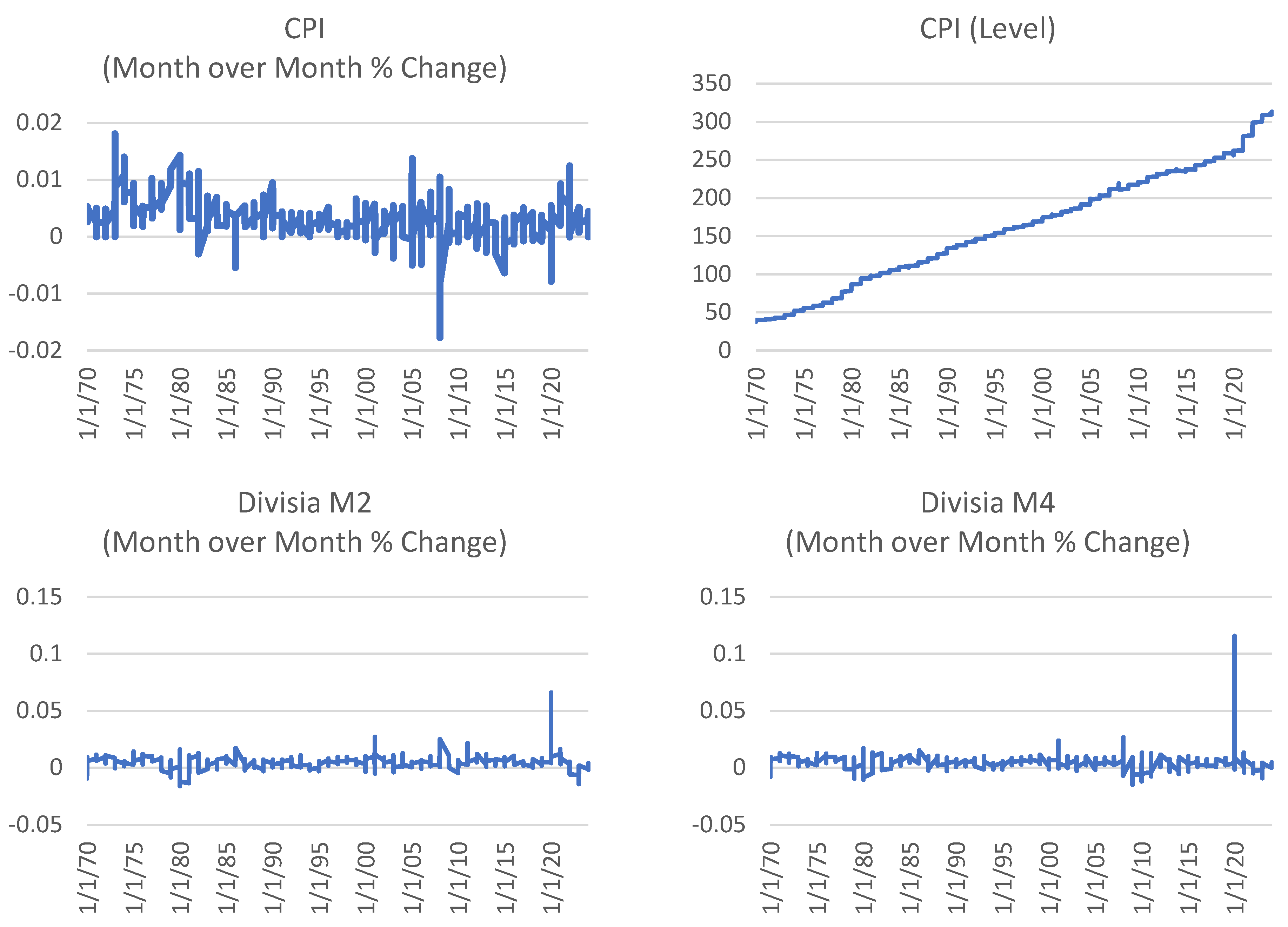
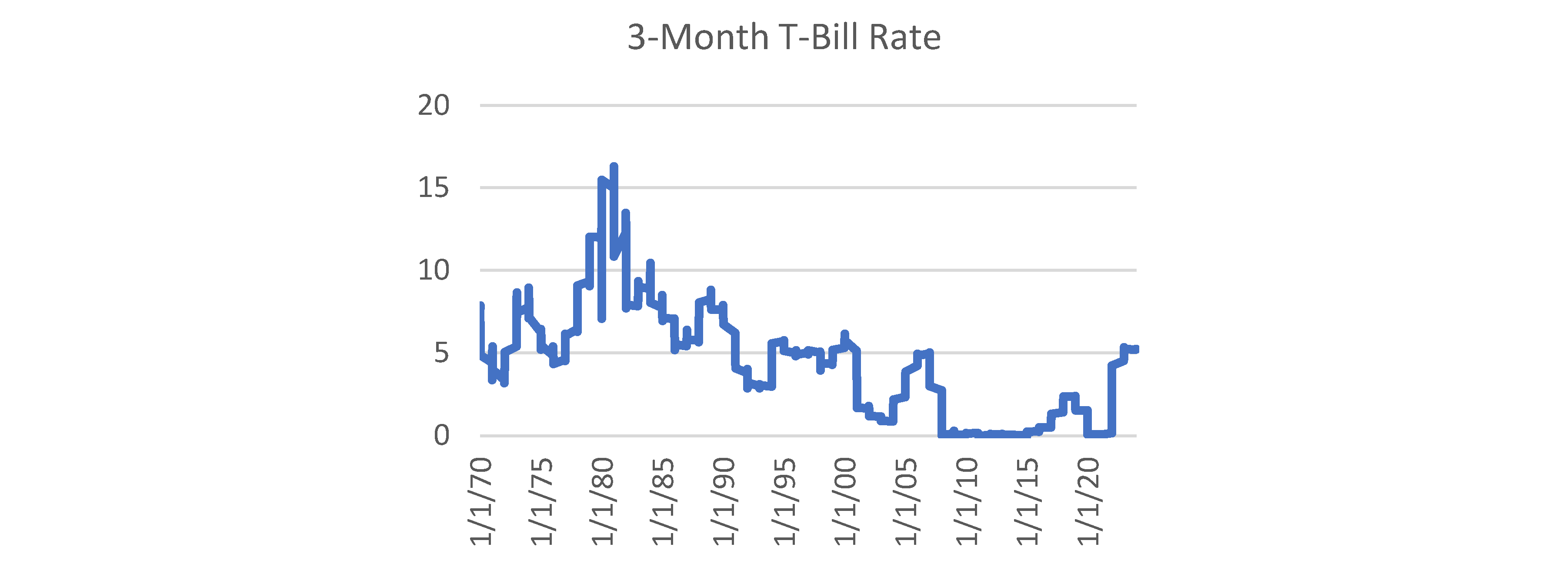
Figure 2.
Multi-recurrent Network Architecture.
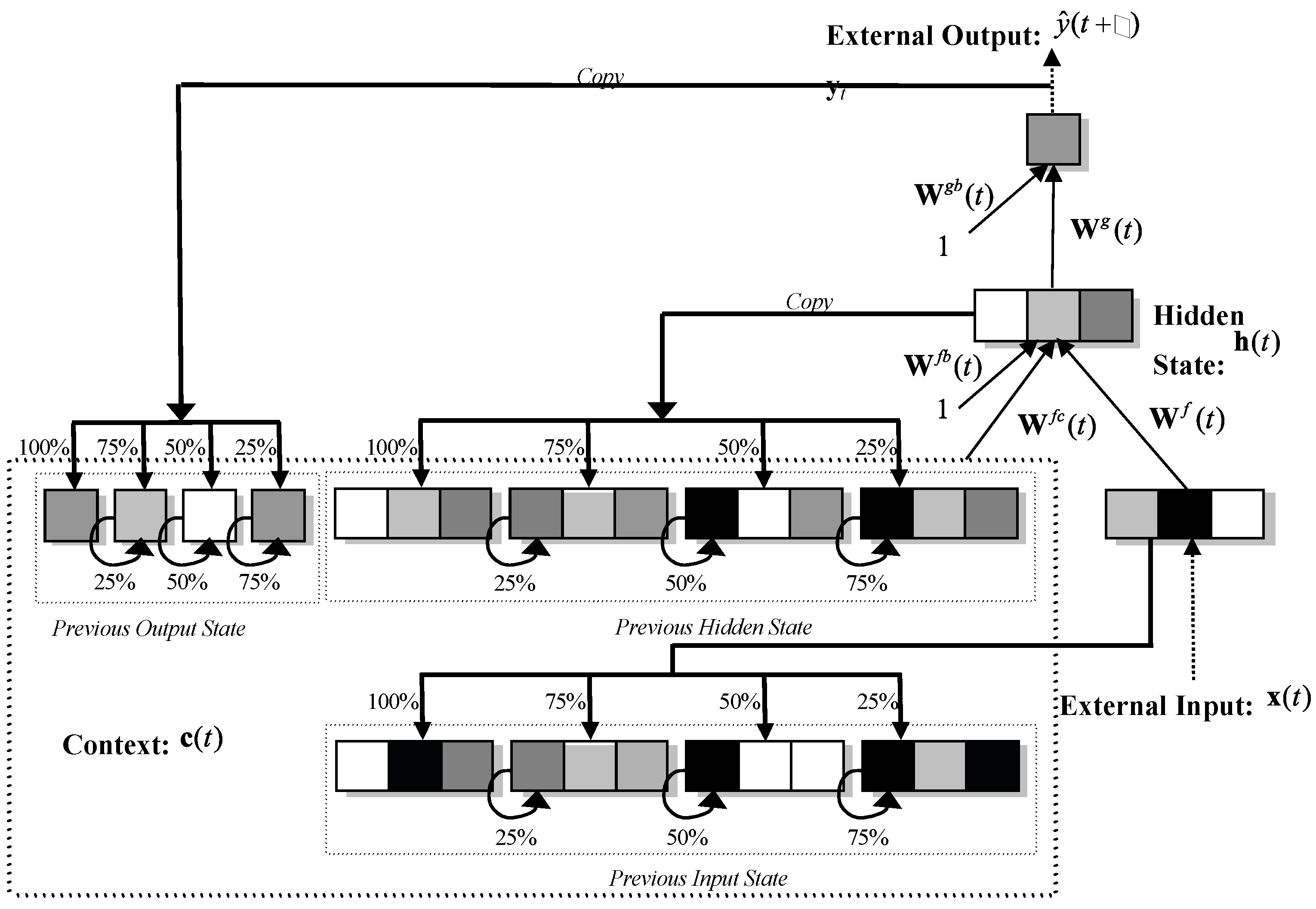
Figure 3.
Multi-recurrent Network Architecture.
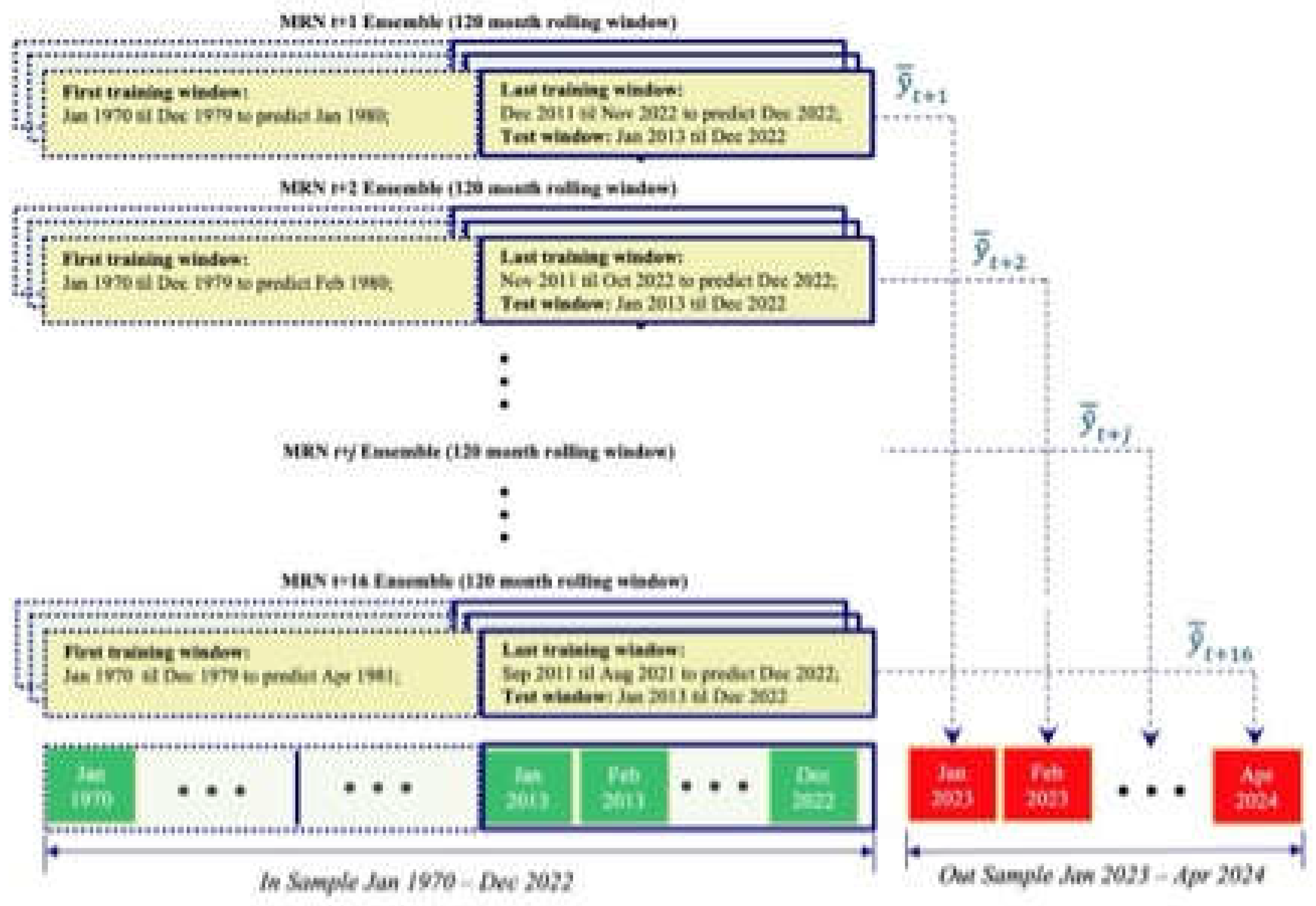
Figure 4.
Comparison of CPI Inflation and Forecasted Values over Time.
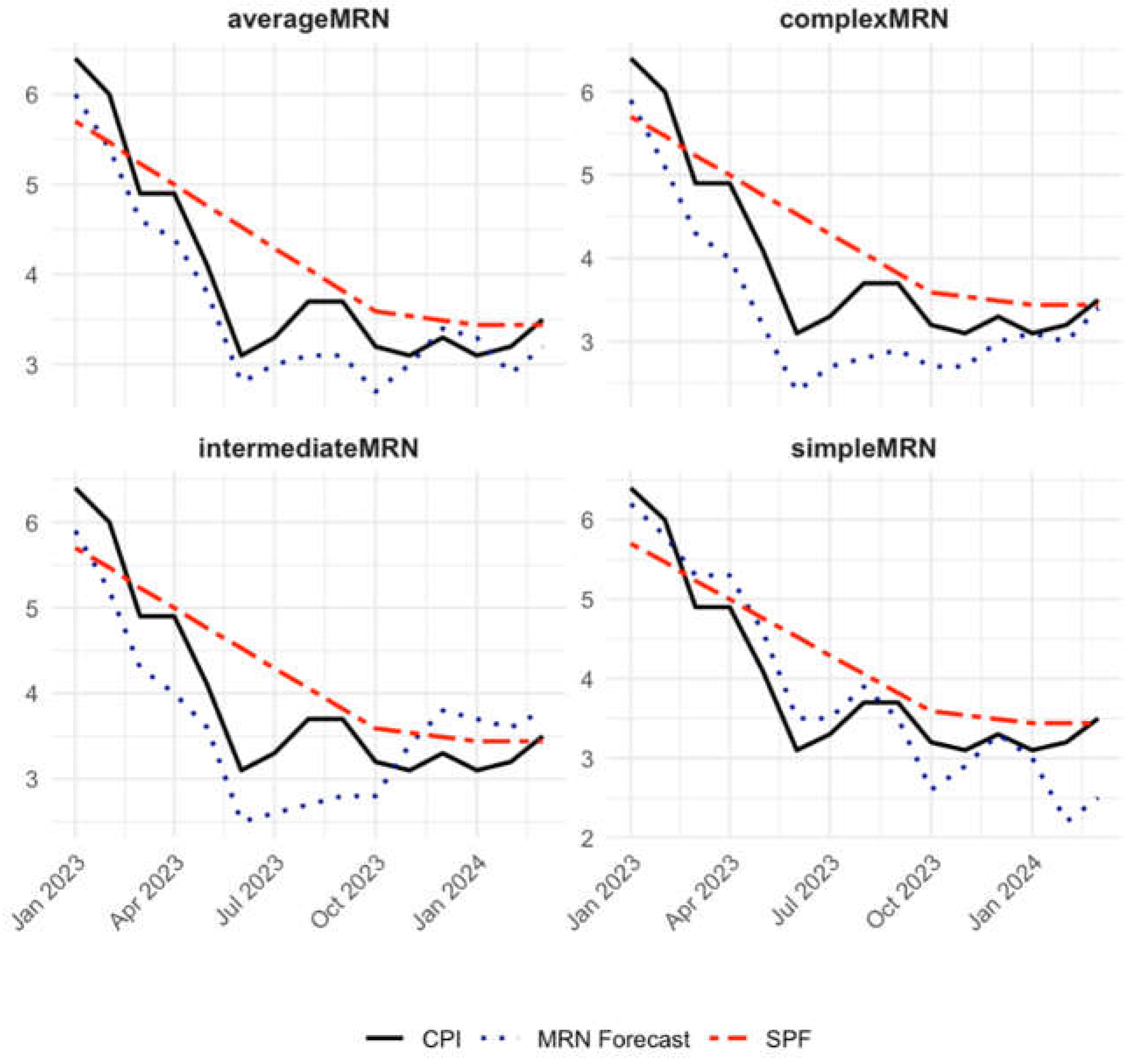

Table 1.
Forecast Model Evaluation Statistics.
| Forecast Method | RMSE | sMAPE |
Theil U Statistic |
Improvement over Random Walk |
| simpleMRN | 0.472 | 10.91% | 0.124 | 0.876 |
| intermediateMRN | 0.637 | 16.47% | 0.167 | 0.833 |
| complexMRN | 0.627 | 15.29% | 0.164 | 0.836 |
| averageMRN | 0.395 | 9.66% | 0.104 | 0.896 |
| SPF | 0.580 | 11.33% | 0.152 | 0.848 |
Disclaimer/Publisher’s Note: The statements, opinions and data contained in all publications are solely those of the individual author(s) and contributor(s) and not of MDPI and/or the editor(s). MDPI and/or the editor(s) disclaim responsibility for any injury to people or property resulting from any ideas, methods, instructions or products referred to in the content. |
© 2025 by the authors. Licensee MDPI, Basel, Switzerland. This article is an open access article distributed under the terms and conditions of the Creative Commons Attribution (CC BY) license (http://creativecommons.org/licenses/by/4.0/).
Copyright: This open access article is published under a Creative Commons CC BY 4.0 license, which permit the free download, distribution, and reuse, provided that the author and preprint are cited in any reuse.


