Inflation Forecasting: LSTM Networks vs. Traditional Models for Accurate Predictions

1. Introduction

Inflation forecasting has been central to macroeconomic research, with traditional models like the Phillips curve offering insights into the relationship between inflation and unemployment. However, these models have shown limitations in capturing the complexities of modern economies. Recent studies suggest that incorporating financial variables, commodity prices, and broader economic indicators can enhance forecasting accuracy (Staiger et al., Atkeson et al., Forni et al., Groen et al. and Chen et al. Atkeson et al. (2001),Chen et al. (2014),Forni et al. (2003),Groen et al. (2013),Staiger et al. (1997)). As central banks increasingly rely on multivariate models to inform monetary policy, the demand for more sophisticated approaches has grown. One well-established approach in inflation forecasting is the use of time series models such as the Stock and Watson multivariate models Stock & Watson (2008). These models integrate a wide range of economic indicators to predict inflation more accurately. However, despite the inclusion of additional variables, these models often struggle to outperform simpler univariate models like SARIMA, out-of-sample. In response to these challenges, machine learning techniques have been applied to inflation forecasting, though with mixed results. Long Short-Term Memory (LSTM) models, for instance, have demonstrated some potential in capturing non-linearities and long-term trends but have not consistently outperformed traditional models like SARIMA Paranhos (2024).

Recent research highlights the importance of model selection and the inclusion of relevant data in improving forecasting performance. Machine learning methods such as Quantile Random Forests Lenza et al. (2023) and LSTM-based models have shown that while these approaches can be powerful, they are also prone to overfitting and lack interpretability, making them less useful for policy applications. This has led to renewed interest in hybrid approaches that combine machine learning with more interpretable models like LASSO to enhance both accuracy and transparency. In this study, we aim to address the limitations of existing machine learning models in inflation forecasting by employing a hybrid model that combines LSTM’s ability to capture long-term dependencies with LASSO’s feature selection capabilities. LASSO helps reduce the dimensionality of the data and focuses on the most relevant variables, thereby enhancing model interpretability and reducing overfitting. By incorporating financial variables and commodity prices alongside traditional economic indicators, we aim to improve forecast accuracy over both short- and long-term horizons. We compare the performance of our LASSO-LSTM model to benchmarks such as univariate models, as well as machine learning techniques.

This study contributes to the literature on inflation forecasting by evaluating the performance of various machine learning models—including Long Short-Term Memory (LSTM) networks, Random Forests, and regularization methods like LASSO regression—in generating plausible inflation forecasts. These complex models are compared to traditional time series models such as Autoregressive (AR(p)) and Seasonal Autoregressive Integrated Moving Average (SARIMA) models. Our findings indicate that, despite the sophisticated capabilities of machine learning models, simpler models like LASSO regression, AR(p), and SARIMA often outperform LSTM networks in forecasting inflation. This is consistent with previous research suggesting that LSTM models may underperform compared to univariate models and other machine learning methods in certain contexts. These results suggest that for policymakers and central bankers seeking reliable and interpretable inflation forecasts, traditional models such as LASSO regression, AR(p), and SARIMA may be more suitable choices. The relative simplicity and transparency of these models can provide clearer insights into inflation dynamics, facilitating more informed decision-making.

The rest of this paper is organized as follows: In section 2 we review relevant literature, section 3 presents the data, section 4 discusses the models, section 5 presents and discusses results whereas section 6 concludes.

2. Literature Review

2.1. Inflation Forecasting with Classical Methods

Inflation-targeting regimes were introduced in many countries in the late 1980s and early 1990s, leading central banks to rely heavily on inflation forecasts for policy decisions. A range of models, including Vector Autoregressive (VAR), Dynamic Stochastic General Equilibrium (DSGE), and factor models, have been employed to guide monetary policy Iversen et al. (2016). During the financial crisis and subsequent recovery, Iversen et al. (2016) found that models like DSGE exhibited forecast biases, whereas Bayesian VAR (BVAR) models performed with less bias, particularly in predicting inflation and interest rates Iversen et al. (2016).

The Phillips curve, which connects inflation and unemployment, has been a foundational model for inflation forecasting. However, Atkeson et al. (2001) demonstrated that Phillips curve models often fail to outperform simpler naive models that predict future inflation based on past trends Atkeson et al. (2001). This criticism has spurred research into alternative approaches, with findings suggesting that Phillips curve models struggle to capture the non-linear dynamics of inflation, especially during periods of significant economic change Fisher et al. (2002).

ARIMA models, though simple, have been shown to perform well for short-term forecasts. Meyler et al. (1998) emphasize that while ARIMA models minimize out-of-sample forecast errors, they lack theoretical grounding and are backward-looking, limiting their ability to predict turning points Meyler et al. (1998). Similarly, Robinson (1998) noted that VAR models are effective at capturing relationships between multiple economic variables and are widely used by central banks Robinson (1998). However, these models can struggle in periods of structural change or economic volatility.

2.2. Inflation Forecasting with Machine Learning

The limitations of traditional models have motivated the exploration of machine learning methods for inflation forecasting. Deep learning models, particularly Long Short-Term Memory (LSTM) networks, have gained attention due to their ability to capture long-term dependencies in data. Theoharidis et al. (2023) argue that LSTM models can outperform traditional methods, particularly at longer horizons, but they also note that deep learning models are prone to overfitting and lack transparency Theoharidis et al. (2023).

Despite their potential, LSTM models have not consistently outperformed simpler models like SARIMA or Random Forest in inflation forecasting. A study by the Bank of England applied LSTM to US inflation data, showing competitive results against other machine learning models such as LASSO and Ridge, but found that the improvements were marginal Paranhos (2024). This suggests that while LSTM is effective at modeling long-term trends, it may not always be the best tool for short-term inflation forecasting, especially when compared to linear models.

The integration of feature selection methods with machine learning has been a promising direction. Garcia et al. (2017) showed that LASSO, a shrinkage method, performs particularly well in data-rich environments, reducing overfitting and improving forecast accuracy for short-term inflation Garcia et al. (2017). By focusing on the most relevant predictors, LASSO-based models can simplify complex datasets and enhance the interpretability of machine learning models.

2.3. The Role of Financial and Commodity Variables in Inflation Forecasting

Stock and Watson (2003) highlighted that asset prices, such as interest rates and stock returns, can serve as useful indicators of future inflation, though their predictive power varies by period and country Stock & Watson (2003). Financial variables, such as spreads and exchange rates, have also been found to be significant contributors to inflation forecasts Forni et al. (2003).

Commodity prices, especially for small commodity-exporting countries, have been shown to have strong predictive power for inflation. Chen et al. (2014) found that world commodity price aggregates outperformed other models, particularly in predicting Consumer Price Index (CPI) and Producer Price Index (PPI) inflation in these economies Chen et al. (2014). The inclusion of such variables has proved to improve the robustness of inflation forecasts, especially in economies highly dependent on commodity exports.

2.4. Motivation for Hybrid Models

Given the challenges of both classical and machine learning models, hybrid approaches that combine the strengths of each have gained prominence. Hybrid models that integrate feature selection techniques like LASSO with deep learning models such as LSTM offer the promise of balance between accuracy and interpretability. These models can allow for the selection of relevant variables, reducing overfitting and improving model performance, particularly in volatile economic conditions. This study builds on this trend by testing a LASSO-LSTM model, incorporating financial variables, and using data augmentation techniques such as Moving Block Bootstrapping (MBB) to enhance out-of-sample performance and robustness.

3. Data

We collected data from the FRED-MD and the EIKON databases. We obtained macroeconomic and financial data from FRED-MD and financial data from EIKON, which provides us with a broad coverage of inflation indicators.

3.1. Variable-Selection

Feature selection is a crucial step in any predictive modeling process, particularly when working with datasets where the number of variables exceeds the number of available samples—a situation commonly referred to as the high-dimensionality problem.

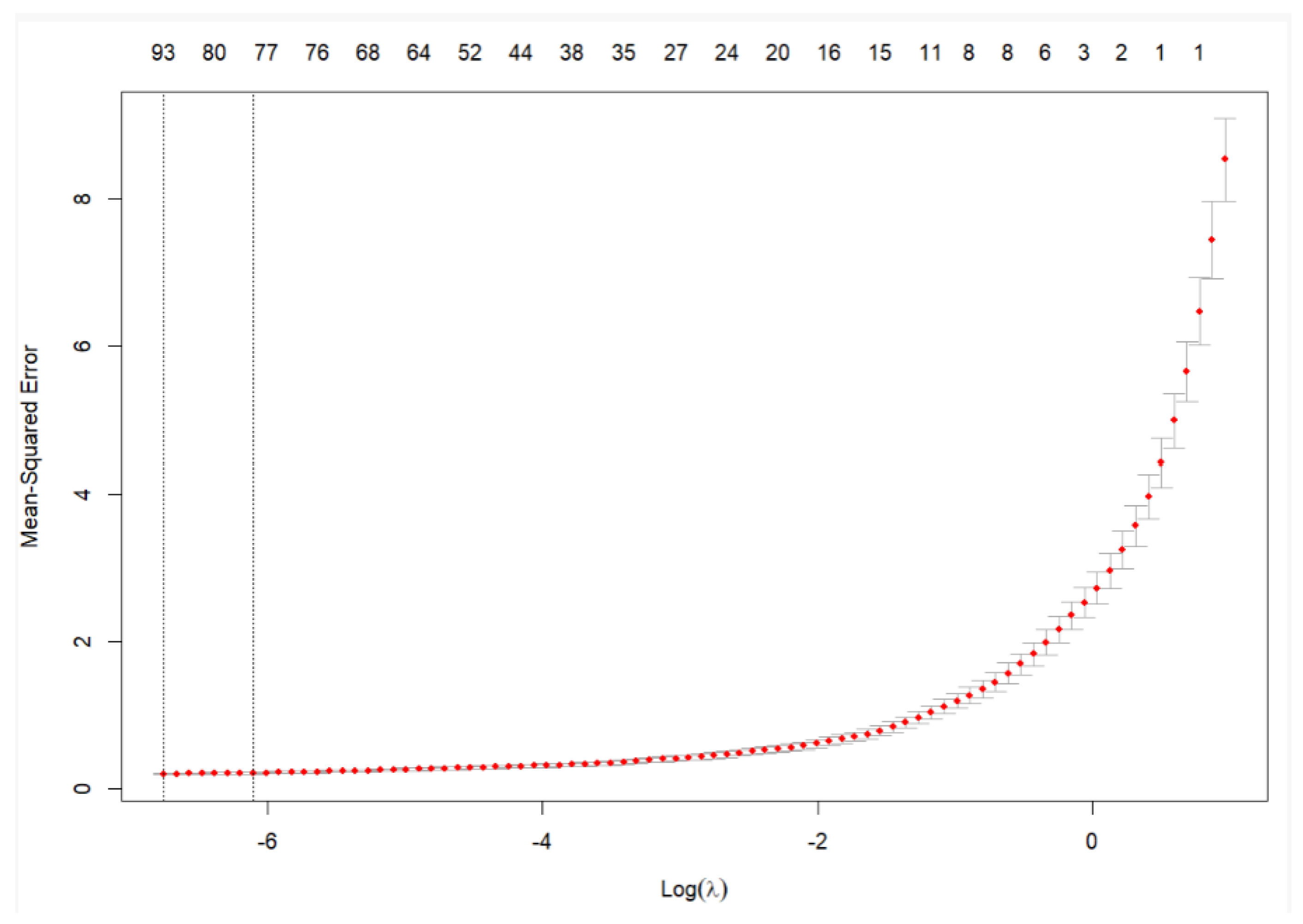
Without proper feature selection, models are at risk of overfitting, leading to poor generalization and unnecessary noise in the results. LASSO addresses this challenge by simultaneously performing variable selection and regularization, reducing the dimensionality of the model while retaining the most significant predictors. As illustrated in Figure 3.1, this method shrinks the coefficients of less important variables to zero, effectively removing them from the model, and thus improving both model performance and interpretability.

Figure 1. LASSO feature selection for a 12 month forecast. The figure illustrates how LASSO selects the most relevant features by shrinking irrelevant coefficients, which is essential for building robust forecasting models that avoid the inclusion of noise and irrelevant data. Without this step, the analysis would be susceptible to overfitting and lack clarity in explaining the underlying relationships within the data.

Figure 1. LASSO feature selection for a 12 month forecast. The figure illustrates how LASSO selects the most relevant features by shrinking irrelevant coefficients, which is essential for building robust forecasting models that avoid the inclusion of noise and irrelevant data. Without this step, the analysis would be susceptible to overfitting and lack clarity in explaining the underlying relationships within the data.

3.2. FRED-MD Database

The FRED-MD dataset contains monthly US data compiled by McCracken and Ng. The data we used were updated in December 2023. This data consists of 128 variables with 768 observations from January 1959 to December 2023.

Some transformation of data were necessary. Variables that are non-stationary have been differenced such that $X_t-X_{t-12}$ represents the annual change in the variable.

We have also treated the dataset for missing data, where missing observations have received the value of the previous observation.

3.3. EIKON Database

We retrieved monthly data for the period January 1960 until December 2023 from the Refinitiv EIKON database. In total we included and combined 27 financial variables from EIKON and FRED-MD to create a new dataset with financial data. Some descriptive statistics are presented in Figure 3.2 below.

Figure 2. Descriptive statistics of financial data.

Figure 2. Descriptive statistics of financial data.

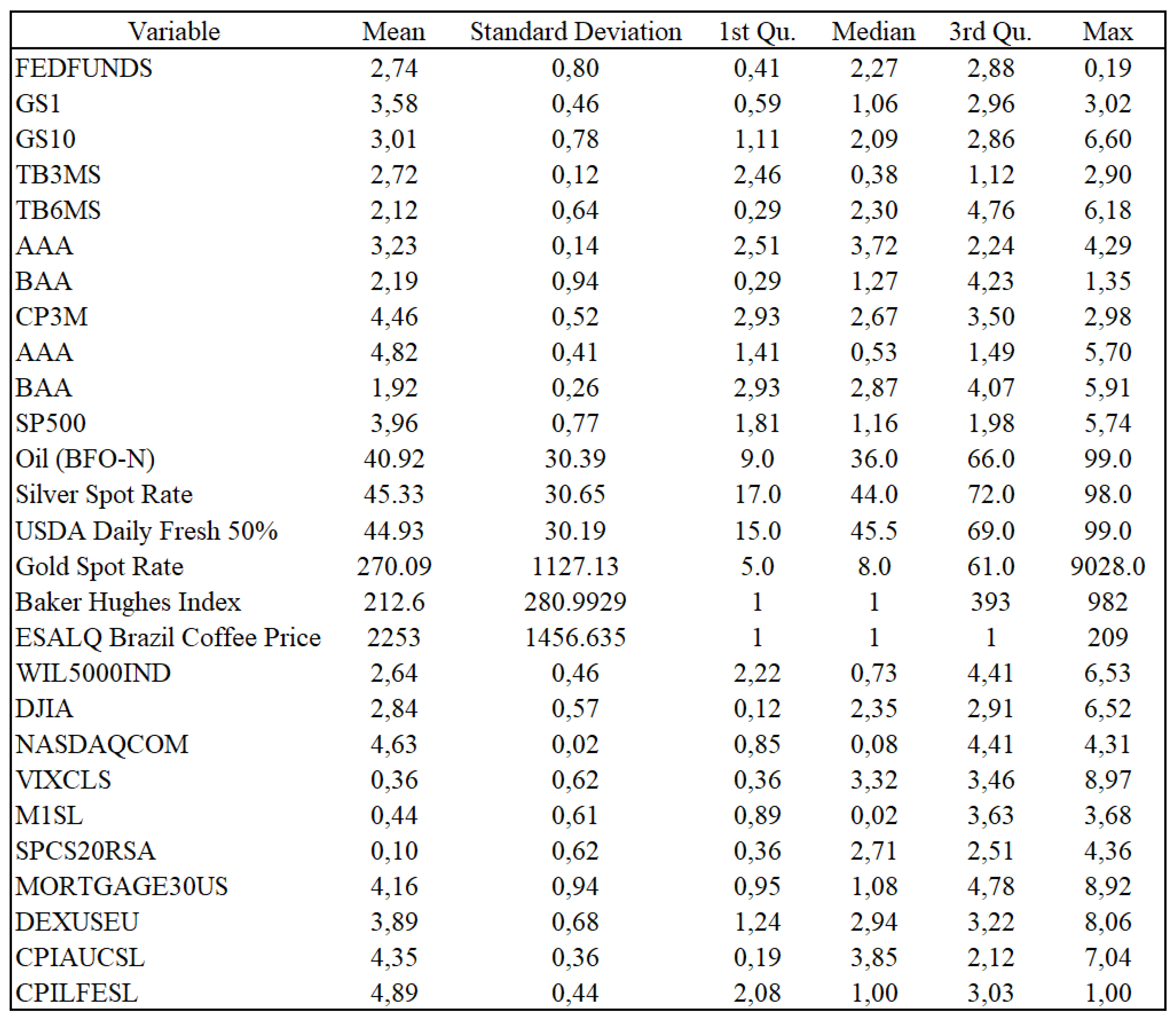
Forni et al. (2003) Forni et al. (2003) and Chen et al. (2014) Chen et al. (2014) emphasize the importance of financial variables and commodity prices in inflation forecasting, and support our belief that including these time series can improve the accuracy of inflation forecasts.

4. Models

4.1. LASSO

Inflation forecasting typically employs huge datasets containing a lot of variables, some of which may be irrelevant for prediction purposes. The Least Absolute Shrinkage and Selection Operator (LASSO) has the ability to select only the most important covariates, discarding irrelevant information and keeping the error of the prediction as small as possible (Freijeiro-González et al., 2022) Freijeiro-González et al. (2022).

LASSO combines properties from both subset selection and ridge regressions. This makes it able to produce explicable models (like subset selection), and be as stable as a ridge regression. The LASSO minimizes the residual sum of squares subject to the sum of the absolute value of coefficients being less than a constant. Because of this constraint LASSO tends to shrink the coefficients on some predictor variables to 0, thus giving us interpretive models (Tibshirani, 1996) Tibshirani (1996). The Lasso model contains:

Data

$$(x^i,y_i),i=1,2,...,N$$

predictor variables

$$x^i={(x_{il},...,x_{ip})}^T$$

and responses

$$y_i$$

We either assume that the observations are independent or that the $y_i$s are conditionally independent given the $x_{ij}$s.

We assume that the $x_{ij}$s are standardized so that:

$$\left({\displaystyle \frac{{\sum }_i{x}_{ij}}{N}}\right)=0,{\displaystyle \frac{{\sum }_i{x}_{ij}^2}{N}}=1$$

Letting $\widehat{B}={(\widehat{B_1},...,\widehat{B_p})}^T,$ the lasso estimate $(\widehat{\alpha },\widehat{B})$ is defined by:

$$(\widehat{\alpha },\widehat{B})=argmin\left[\sum _{i=1}^N{(y_i-\alpha -\sum _j{\beta }_j{x}_{ij})}^2\right]$$

Subject to

$$\sum _j\left|{\beta }_j\right|⩽t$$

Here $t\ge 0$ is a tuning parameter. Now, for all t, the solution for $\alpha$ is $\widehat{\alpha }=\overline{y}$ . We can assume without loss of generality that $\overline{y}=0$ and hence omit $\alpha$.

The parameter $t\ge 0$ controls the amount of shrinkage that is applied to the estimates. Let $\widehat{B_j^0}$ be the full least squares estimates and let $t_0=\sum \left|\widehat{B_j^0}\right|$. Values of $t<t_0$ will cause shrinkage of the solutions toward 0, and some coefficients may be exactly equal to 0. For example, if $t=t_0/2$ the effect will be roughly similar to finding the best subset of size $p/2$. The design matrix does not need to be of full rank (Tibshirani, 1996) Tibshirani (1996)

The reason for including LASSO in our model is to tackle the problems of overfitting and optimism bias. A LASSO regression tries to identify variables and corresponding regression coefficients that constitute a model that minimizes prediction error. This is done by imposing a constraint on the model parameters, shrinking the regression coefficient towards zero, forcing the sum of the absolute value of the regression coefficients to be less than a fixed value ($\lambda$).

$$(\widehat{\alpha },\widehat{B})=argmin[\sum _{i=1}^N{(y_i-\alpha -\sum _j{\beta }_j{x}_{ij})}^2+\lambda \sum _j|{\beta }_j|]$$

After the shrinkage, variables with regression coefficients equal to zero are excluded from the model (Ranstam and Cook, 2018) Ranstam & Cook (2018).

We use an automated k-fold cross-validation approach for choosing $\lambda$. To obtain this the dataset is randomly partitioned into k sub-samples of the same size. When k-1 sub-samples are used for developing a prediction model, the remaining sub-sample is used to validate this model. This is done k times, with each of the k sub-samples in turn being used for validation and the other for model development. By combining the k separate validation results for a range of $\lambda$ values and choosing the preferred $\lambda$ we get the results that are used to determine the final model.

This technique reduces overfitting without the need to reserve a subset of the dataset exclusively for internal validation. A disadvantage of the LASSO approach is that one may not be able to reliably interpret the regression coefficients in terms of independent risk factors, since the focus is on the best combined prediction, and not on the accuracy of the estimation (Ranstam and Cook, 2018) Ranstam & Cook (2018).

4.2. LSTM

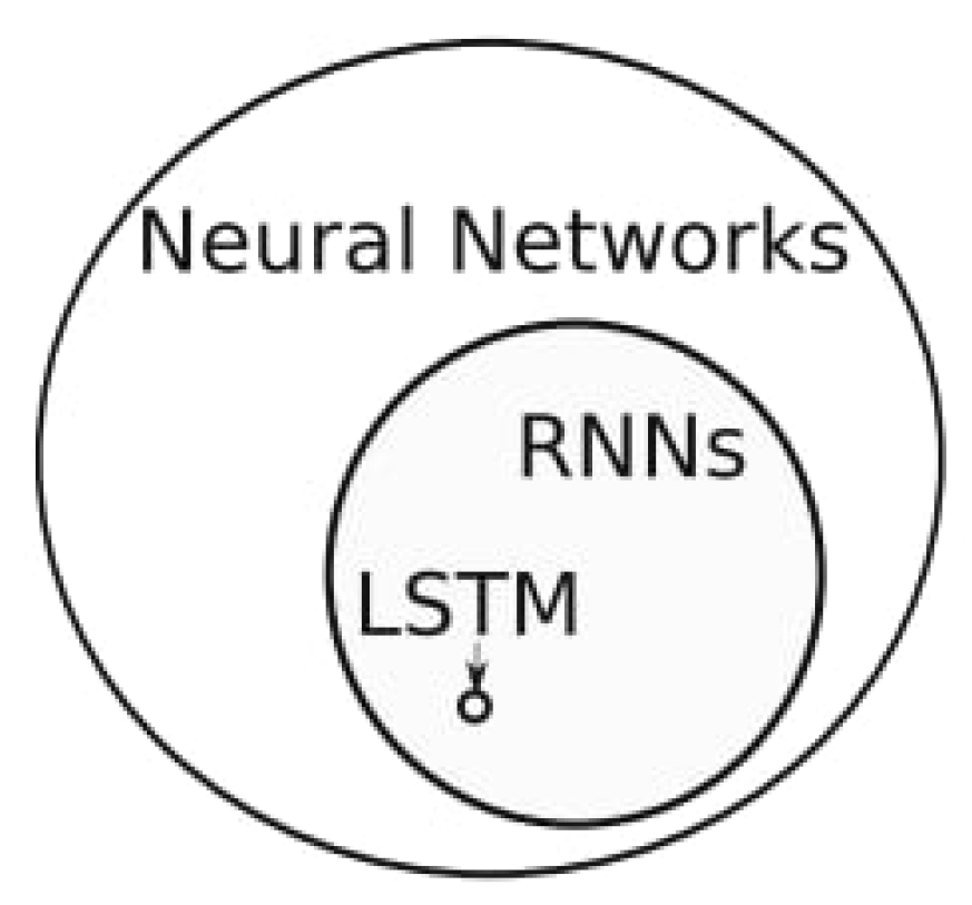
As depicted in Figure 4.2, the LSTM model is a variant of recurrent neural networks (RNNs) Almosova & Andresen (2023). Unlike other neural networks, a recurrent neural network updates by time step. This means that the model will adjust forecasts based on previous time steps. RNN models have proven particularly useful for data-sensitive sequences such as time series analysis, natural language processing and sound recognition (Mullainathan and Spiess, 2017) Mullainathan & Spiess, 2017). For example, in the context of music recognition one could observe a pattern in the sound, making it possible to predict what is to come next or which song you are listening to (Bishop, 2006) Bishop, 2006). For such models it is crucial that there is a pattern in the data, and that the sequence of the data anticipates later values.

The RNN model is able to update its memory based on previous steps and consider long term trends and patterns in the data (Tsui et al., 2018) Tsui et al. (2018). Consider an abnormal drop in inflation for one month, deviating with previous time steps in the data. The RNN takes into account the underlying pattern in the data based on previous observations, and considers the fall in inflation as an abnormality. What makes inflation behavior abnormal, and which patterns the model detects to label the drop in inflation as abnormal, is inherently difficult to grasp.

Figure 3. Classification of neural networks. LSTM is a specific type of recurrent neural network (RNN) within the broader group of neural networks (Almosova and Andresen, 2023) Almosova & Andresen (2023).

Figure 3. Classification of neural networks. LSTM is a specific type of recurrent neural network (RNN) within the broader group of neural networks (Almosova and Andresen, 2023) Almosova & Andresen (2023).

LSTM on the other hand, differs from other RNNs as it possesses an enhanced capability of capturing long term trends in the data Tsui et al. (2018). Consider an inflationary event in the 1970s that has a similar pattern as one observed recently. The LSTM will observe the similarities in pattern of the two events, and take this into account when making its next prediction. It is important to state that the event occurring in the 70s will not be fully weighted, but adjusted for short term events seen in the data. LSTM thus has the ability to consider both distant and recent events, when making its predictions (Lenza et al., 2023) Lenza et al. (2023).

LSTM has proven to be highly efficient for sequential data and has been used to compute univariate forecasts of monthly US CPI inflation. LSTM slightly outperforms autoregressive models (AR), Neural Networks (NN), and Markov-switching models, but its performance is on par with the SARIMA model (Almosova and Andresen, 2023) Almosova & Andresen (2023). Recently, it has become harder to outperform naive univariate random walk-type forecasts of US inflation, but since the mid-80s, inflation has also become less volatile and easier to predict. Atkeson and Ohanian Atkeson et al. (2001) show that averaging over the last 12 months gives a more accurate forecast of the 12-month-ahead inflation than a backwards looking Phillips curve. Macroeconomic literature argues that the inflation process might be changing over time, making a nonlinear model more precise in predicting inflation. According to Almosova and Andresen Almosova & Andresen (2023) there are four main advantages of the LSTM method.

1. LSTMs are flexible and data-driven. It means that researchers do not have to specify the exact form of the non-linearity. Instead, the LSTM will infer this from the data itself.

2. Under some mild regulatory conditions LSTMs and neural networks of any type in general can approximate any continuous function arbitrarily accurately. At the same time, these models are more parsimonious than many other nonlinear time series models.

3. LSTMs were developed specifically for the sequential data analysis and have proved to be very successful with this task.

4. The recent development of the optimization routines for NNs and the libraries that employ computer GPUs made the training of NNs and recurrent neural networks significantly more feasible.

In contrast to classical time-series models, the LSTM-network does not suffer from data instabilities or unit root problems. Nor does it suffer from the vanishing gradient problem of general RNNs, which can destroy the long-term memory of these networks. LSTM may be applied to forecasting any macroeconomic time-series, provided that there are enough observations to estimate the model.

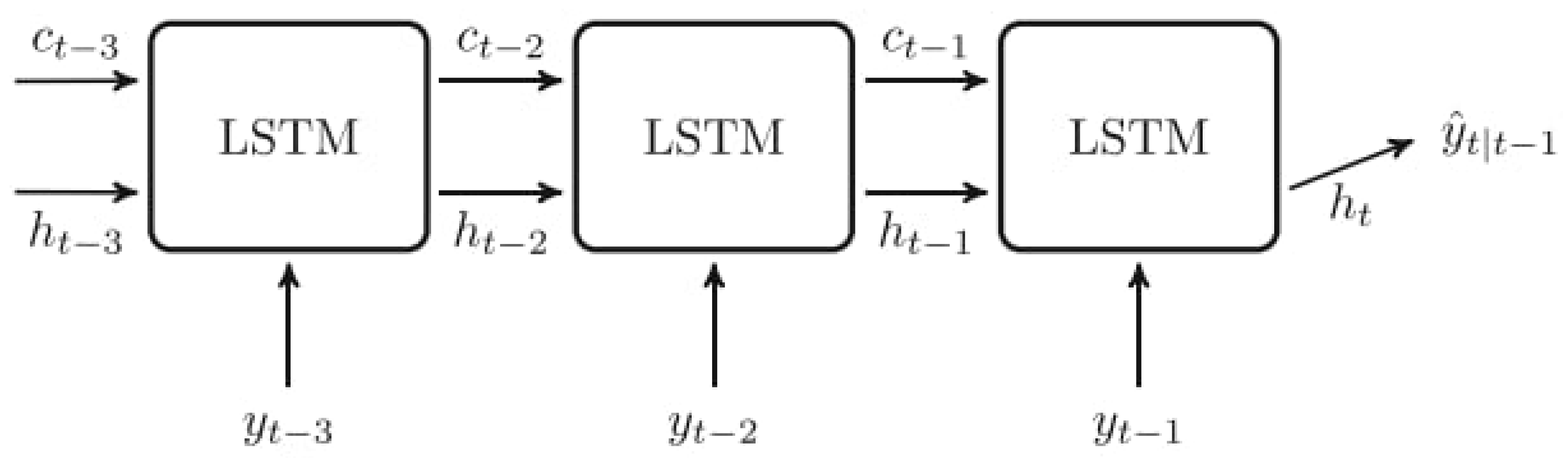
Theoretically, Convolutional Neural Networks (CNN), originally developed for images, could also be used for time series forecasting, if one treats the input as a one-dimensional image. LSTMs performs particularly well at long horizons and during periods of high macroeconomic uncertainty. This is due to their lower sensitivity to temporary and sudden price changes compared to traditional models in the literature. One should note that their performance is not outstanding, for instance compared to the random forest model (Lenza et al., 2023) Lenza et al. (2023). Neural nets as well demonstrate competitive, but not outstanding, performance against common benchmarks, including other machine learning methods. A simlified, visual representation of an LSTM recurrent structure is provided in Figure 4.2.

Figure 4. Representation of LSTM recurrent structure. LSTM has a cell state $\left(c_t\right)$ and a hidden state $\left(h_t\right)$. As t increases, more information $\left(y\right)$ is put into the cell state and memory state. This new information in the cell and memory state contribute to the prediction $\left(h\right)$ (Almosova Andresen, 2023) Almosova & Andresen (2023).

Figure 4. Representation of LSTM recurrent structure. LSTM has a cell state $\left(c_t\right)$ and a hidden state $\left(h_t\right)$. As t increases, more information $\left(y\right)$ is put into the cell state and memory state. This new information in the cell and memory state contribute to the prediction $\left(h\right)$ (Almosova Andresen, 2023) Almosova & Andresen (2023).

A common weakness of machine learning techniques, including neural networks, is the lack of interpretability (Mullainathan and Spiess, 2017) Mullainathan & Spiess (2017). For inflation in particular this could be a problem, since much of the effort is devoted to understanding the underlying inflation process, sometimes at the expense of marginal increases in forecasting gains. LSTM is on average less affected by sudden, short-lived movements in prices compared to other models. Random forest has proved sensitive to the downward pressure on prices caused by the global financial crisis (GFC). Machine learning models are more prone to instabilities in performance due to their sensitivity to model specification (Almosova and Andresen, 2023) Almosova & Andresen (2023). This also applies to the LSTM-network. Lastly, LSTM-implied factors display high correlation with business cycle indicators, informing on the usefulness of such signals as inflation predictors.

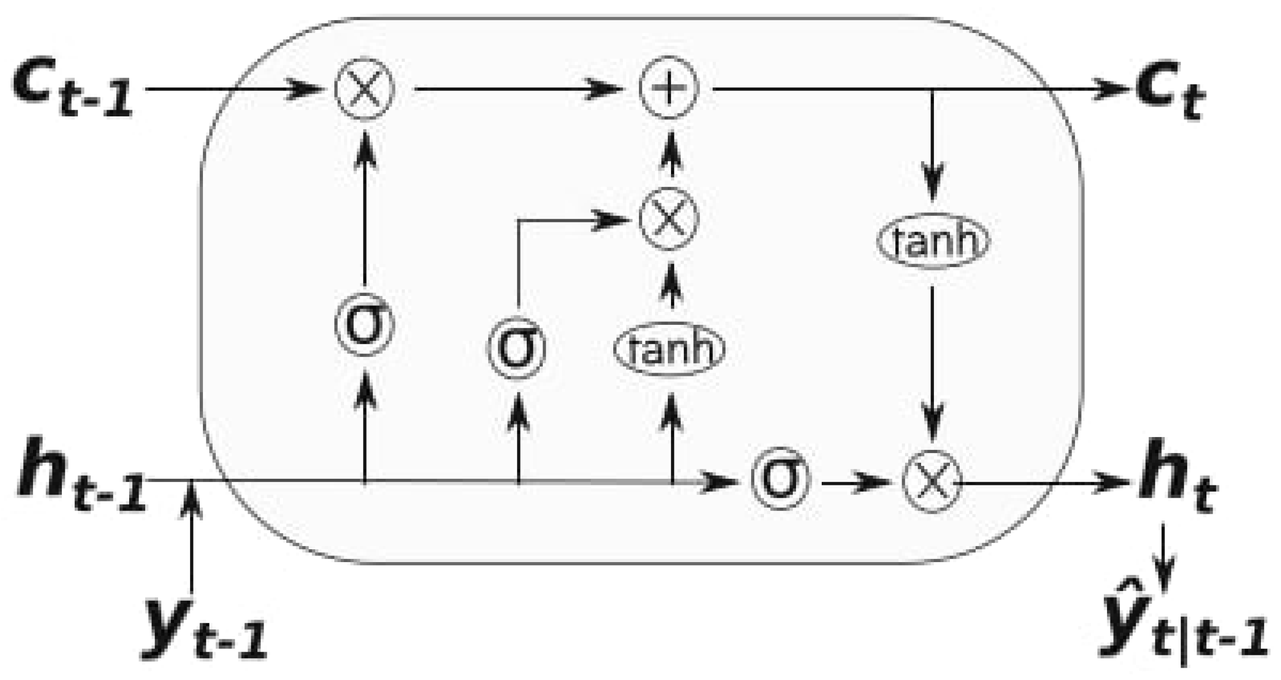
The LSTM model can be described by the cell state function and the internal memory. A visual representation of an LSTM cell is provided in Figure 4.3. These functions start out with their initial value, before new information attained from new observations enter and impact the value of the function. We apply the sigmoid and tanh function, giving us the updated values of the internal memory and cell state.

Figure 5. The figure illustrates the schematic of an LSTM cell. The cell state $c_{t-1}$ and hidden state $h_{t-1}$ from the previous time step, along with the current input $y_{t-1}$, are processed through forget, input, and output gates. The forget gate determines how much of the previous cell state should be retained, while the input gate decides how much new information should be added. These combined results update the cell state $c_t$. The output gate determines the next hidden state $h_t$, which, combined with the updated cell state, forms the output $y_{t|t-1}$. Activation functions like tanh and sigmoid are used to regulate the flow of information within the cell, ensuring that the LSTM effectively captures long-term dependencies in the data (Almosova and Andresen, 2023) Almosova & Andresen (2023).

Figure 5. The figure illustrates the schematic of an LSTM cell. The cell state $c_{t-1}$ and hidden state $h_{t-1}$ from the previous time step, along with the current input $y_{t-1}$, are processed through forget, input, and output gates. The forget gate determines how much of the previous cell state should be retained, while the input gate decides how much new information should be added. These combined results update the cell state $c_t$. The output gate determines the next hidden state $h_t$, which, combined with the updated cell state, forms the output $y_{t|t-1}$. Activation functions like tanh and sigmoid are used to regulate the flow of information within the cell, ensuring that the LSTM effectively captures long-term dependencies in the data (Almosova and Andresen, 2023) Almosova & Andresen (2023).

4.3. LASSO-LSTM

The LASSO-LSTM model is an integrated machine learning, neural network model. It integrates the strengths of LASSO and LSTM. The initial step is LASSO, for feature selection. Predictors are fitted, reducing errors of the residuals in a similar fashion to that of OLS. LASSO applies a shrinkage parameter ($\lambda$) to the coefficients, shrinking the size of less significant predictors. The size of the hyper-parameter ($\lambda$) is important, as it decides the number of predictors that the LSTM model will be trained on.

The regularisation term of LASSO has the function of feature selection. The predictors that are determined to be most significant will not receive large penalties to their coefficients, rendering them important in the forecasting of inflation. The regularisation term is set to three sizes. In this study LASSO-LSTM is constructed with three sizes of architecture, large, medium and small. Increasing the regulatization term size results in a smaller LASSO-LSTM architecture. This approach will contribute in assessing how to balance underfitting and overfitting, in the context of macro-economic forecasting.

When dealing with medium sized sample datasets and high dimensional data, the LSTM model, while known to handle dimensionality well, can run into problems of overfitting. Work done on LSTM for macroeconomic forecasting has shown that larger architectures do not necessarily outperform smaller ones (Paranhos, 2024) Paranhos (2024). Feature selection performed by LASSO detects the features that can contribute to the forecasting performance of the LSTM.

The features considered most important after regularisation, proceed to the LSTM input layer. Different sizes of architectures have different amounts of layers. Larger architectures, more prone to overfitting, receive fewer layers of fully connected nodes, and receive drop out layers. Smaller architectures, less prone to overfitting, can have more layers and/or fewer dropout layers. The LSTM layer structures can then be trained on forecasting inflation based on the number of predictors deemed most important by LASSO. The LASSO-LSTM model, as an augmented version of the LSTM model integrating feature selection, contributes to model regularization.

An alternative approach commonly used for feature selection, is principal component analysis (PCA) (Tsui et al., 2028) Tsui et al. (2018). The two approaches deviate in their goals. PCA deems variables important based on variance. LASSO, by shrinking coefficients, retains the variables considered important. Thus LASSO-LSTM retains some interpretability, as forecasts are based on important factors, which is of interest to central banks in their decision making.

4.4. ARIMA and SARIMA

SARIMA, Seasonal Autoregressive Integrated Moving Average, is an extension of ARIMA, which supports the direct modeling of the seasonal component of a time series. ARIMA does not support a time series with a repeating cycle, and it expects that data is either non-seasonal or that the seasonal component is removed, for example through seasonal differencing (Dubey et al., 2021) Dubey et al. (2021).

An ARIMA(p, d, q) model can be represented by Equation (1) below:

$$\begin{array}{cc}\hfill {\Delta }^d{Y}_t& ={\beta }_0+\sum _{i=1}^p{\varphi }_i{Y}_{t-i}+\sum _{j=1}^q{\theta }_j{e}_{t-j}+e_t\hfill \end{array}$$

(1)

Here ${\beta }_0$ is a constant, ${\varphi }_i$ are the coefficients of the autoregressive part with p lags, ${\theta }_j$ are the coefficients of the moving average part with q lags and $e_t$ is the error term at time t. The error terms are typically assumed to be i.i.d. variables drawn from a normal distribution with zero mean.

The model involves a linear combination of lags, and the goal is to identify the optimal p, d, and q values. The minimum difference (d) is selected in the order by which the autocorrelation reaches zero. The p is determined by the order of the AR-term, and should be equal to the lags in the PAC, which significantly crosses the limit set. Equation (2) shows the Partial Autocorrelation (PAC), where y is considered the response variable and $x_1$, $x_2$, and $x_3$ are the predictor variables. The PAC between y and $x_3$, (2), is calculated as the correlation between the regression residuals of y on $x_1$ and $x_2$ with the residuals of $x_3$ on $x_1$ and $x_2$.

$$\begin{array}{cc}\hfill PAC& ={\displaystyle \frac{\mathrm{cov}(\left.y,x_3\right|x_1,x_2)}{\sqrt{\mathrm{var}\left(y\right|x_1,x_2)·\mathrm{var}\left(x_3\right|x_1,x_2)}}}\hfill \end{array}$$

(2)

The $h^{th}$ order partial autocorrelation can be represented as (3):

$$\begin{array}{cc}\hfill PA{C}^h& ={\displaystyle \frac{\mathrm{cov}(y_i,y_{i-h}|y_{i-h+1},\dots ,y_{i-1})}{\sqrt{\mathrm{var}\left(y_i\right|y_{i-1},\dots ,y_{i-h+1})·\mathrm{var}\left(y_{i-h}\right|y_{i-1},\dots ,y_{i-h+1})}}}\hfill \end{array}$$

(3)

The q is calculated based on the Autocorrelation (AC) and denotes the error of the lagged forecast:

$$\begin{array}{cc}\hfill AC& ={\displaystyle \frac{{\sum }_{i=1}^{N-k}(y_i-\overline{y})(y_{i+k}-\overline{y})}{{\sum }_{i=1}^N{(y_i-\overline{y})}^2}}\hfill \end{array}$$

(4)

Here,

• $\overline{y}$: The mean of the time series
• k: The lag, where $k\ge 0$
• N: The complete series value

If one requires seasonal patterns in the time series, a seasonal term can be added, which produces a SARIMA model. This model can be written as (5):

$$\begin{array}{c}\hfill ARIMA(p,d,q)\ast (P,D,Q)s\end{array}$$

(5)

Here (p,d,q) represent the non-seasonal part, and (P,D,Q) represents the seasonal part of the model. S represents the period number in a season. In this study we employ SARIMA as we assume there exists seasonality in inflation data.

A seasonal ARIMA model uses differencing at a lag equal to the number of seasons (s) to remove additive seasonal effects. As with lag 1 differencing to remove a trend, the lag s differencing introduces a moving average term. The seasonal ARIMA model includes autoregressive and moving average terms at lag s. The trend elements can be chosen through careful analysis of AFF and PACF plots looking at the correlations of recent time steps. Similarly, ADC and PACF plots can be analyzed to specify values for the seasonal model by looking at correlation at seasonal lag time steps.

In short, SARIMA supports univariate time series data with a seasonal component, and adds three new hyper-parameters to specify the autoregression (AR), differencing (I) and moving average (MA) for the seasonal component of the series, as well as an additional parameter for the period of the seasonality. The reason for comparing NNs with SARIMA is that their celebrated performance might be due to their ability to capture seasonality. Consequently NNs should be compared to a linear seasonal model. Often economic time series variables evolve in a cyclical pattern through time, i.e., exhibit seasonality. In relation to inflation, sales, holidays, and production cycles can cause seasonal price variations that affect the Consumer Price Index.

According to most of the literature on inflation forecasting, SARIMA is the top performing classical model and usually outperforms VAR, AR and ARIMA (Paranhos, 2024) Paranhos (2024). Also, compared to the newer machine learning methods like Recurrent neural networks, LSTM and feed forward neural networks, SARIMA performs on par or better. This makes the SARIMA model a natural choice for our main benchmark, as we want to compare machine learning methods to classical methods, as well as look for ways to improve these methods.

4.5. Benchmark

To determine the performance of the LASSO-LSTM model, we employ standard benchmarks from the literature. These are the autoregressive model (AR(p)), the seasonal autoregressive integrated moving average (SARIMA), the random forest (RF) and the least absolute shrinkage and selection operator (LASSO). To evaluate out of sample performance, the models have been trained on two sets of data. Forecasts for the period of 2010 to 2023 are produced by models trained on data from 1960 to 2010, whereas forecasts for the period of 1997 to 2009 are produced by models trained on data for the period from 1960 to 1997.

Forecasts are evaluated against actual values by RMSE tests. We then compare the LASSO-LSTM model to the benchmark models using the Diebol-Mariano (DM) test.

4.6. Network Training

4.6.1. LSTM

We start by splitting the data into training data, two validation sets, and an out-of-sample set. The training and validation data cover the period from 1960 to 1997, and are used to train the model. The out-of-sample data ranges from 2010 to the end of 2023.

The first step is the tuning of the model, and starts with a set of hyper-parameters, which the model applies to create thousands of epocs.

The epochs are tested on the first validation set, and the best performing epoch is tested on a second validation set. This procedure is repeated several times with different sets of hyper-parameters. All selected epochs are compared on a second validation set, and the best tuned one is retained and applied to the out-of-sample set.

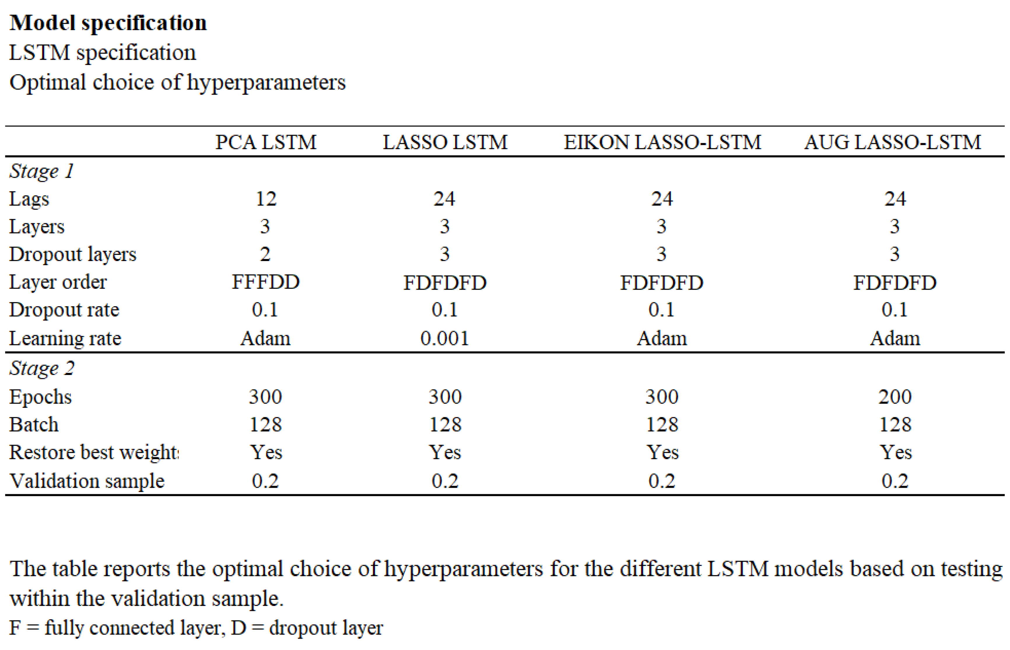
We refer readers to Figure 4.4 for the specifications related to the different models.

Feature selection occurs prior to model tuning, and is performed using LASSO and PCA. The features for both LASSO-LSTM and PCA-LSTM are based on the training data and the first validation sample. The specification of the LSTM model can be divided into four distinct parts:

1) Feature selection: Features are selected based on their relevance to the data and the problem at hand. This is an independent step that occurs before training and optimization.

2) Model configuration: This involves setting a range of structure and parameters for the LSTM model, including the incorporation of lagged versions, the number and order of layers, the number of dropout layers, the dropout rate percentage, and the learning rate.

3) Training and optimization: This step includes setting the number of epochs, batch sizes, and validation strategies.

4) Model evaluation: This involves comparing different versions of the LSTM model and selecting the best one based on performance metrics.

Figure 6. The table presents the optimal specifications for the applied LSTM models, showing the best values for hyper-parameters such as lags, layers, dropout layers, dropout rate, learning rate, epochs, batch size, and validation sample.

Figure 6. The table presents the optimal specifications for the applied LSTM models, showing the best values for hyper-parameters such as lags, layers, dropout layers, dropout rate, learning rate, epochs, batch size, and validation sample.

4.6.2. Other Machine Learning Models

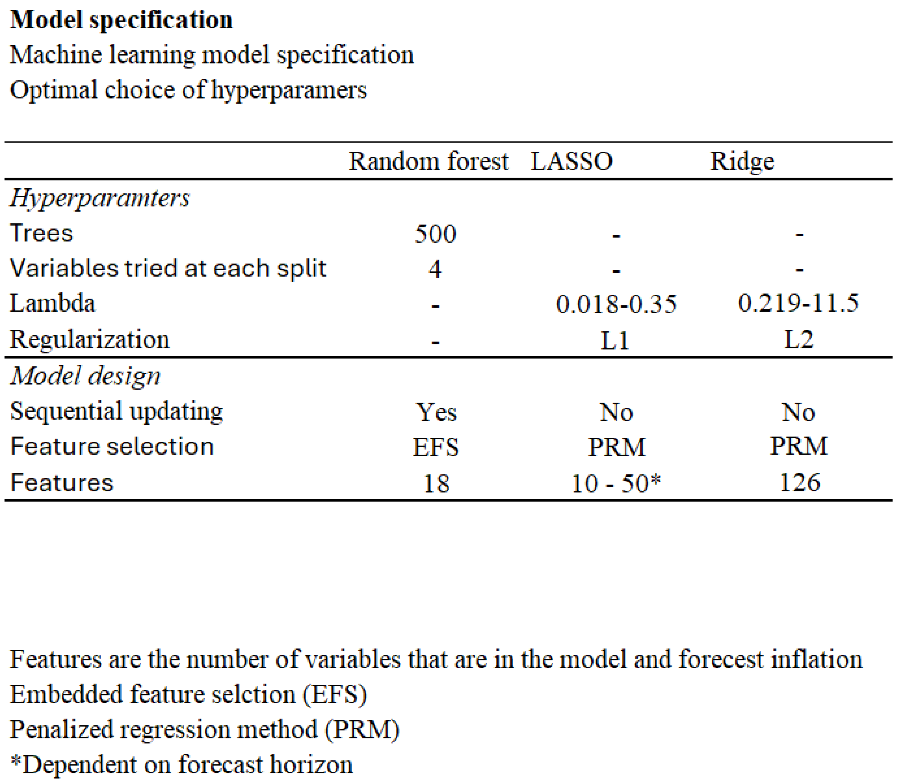
The data for the other machine learning models employed in this study is split into three parts; training, validation and out-of-sample. Data from 1960 to 2010 is used for training and validation. Figure 4.5 gives an overview of the optimal hyperparameters selected for these models.

The first step is embedded feature selection, where features are selected to be included in the model using training data and the validation sample. This process is crucial for the Random Forest algorithm.

Unlike the other models, Random Forest has been specified to sequentially update. This means that each forecast utilizes all available data up to a certain point in time. As new forecasts are made, more data is incorporated into the model. The process of sequential updating allows the Random Forest to continually fit the available data, ensuring that the model remains up-to-date with the most recent information. However, the initial feature selection and hyper-parameters chosen during training remain constant throughout the forecasting period. This approach ensures that the Random Forest model is both dynamic and robust, adapting to new data while maintaining a consistent set of features and hyper-parameters.

LASSO and Ridge regression models are also trained and fitted using the training and validation samples, with the penalty term optimized based on the validation sample performance.

After determining the best model specifications, these models are tested on out-of-sample data.

Figure 7. Optimal hyper-parameters and model specifications for Random Forest, LASSO, and Ridge regression models. Random Forest uses 500 trees and 4 variables per split, with sequential updating and Embedded Feature Selection (EFS) incorporating 18 features. LASSO applies a lambda range of 0.018-0.35 with an L1 penalty, using Penalized Regression Method (PRM) with 10-50 features and no sequential updating. Ridge regression uses a lambda range of 0.219-11.5 with an L2 penalty, employing PRM with 126 features and no sequential updating.

Figure 7. Optimal hyper-parameters and model specifications for Random Forest, LASSO, and Ridge regression models. Random Forest uses 500 trees and 4 variables per split, with sequential updating and Embedded Feature Selection (EFS) incorporating 18 features. LASSO applies a lambda range of 0.018-0.35 with an L1 penalty, using Penalized Regression Method (PRM) with 10-50 features and no sequential updating. Ridge regression uses a lambda range of 0.219-11.5 with an L2 penalty, employing PRM with 126 features and no sequential updating.

4.6.3. Univariate Time Series Models

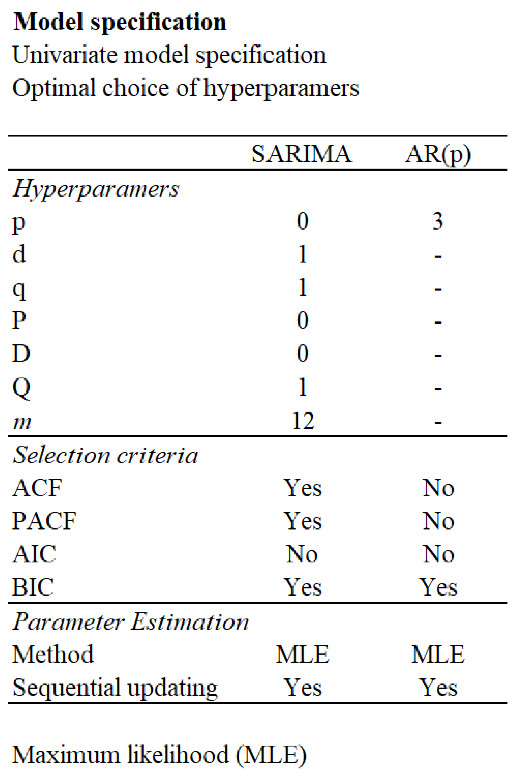
The specification of the AR(p) model was based on results from the ACF, PACF and BIC. The SARIMA model was determined based on the same tests. Both approaches use maximum likelihood, and other approaches were not tested. Both time series models are sequentially updated as forecasts are made, adjusting only the coefficients of the model, not the hyper-parameters. The optimal hyperparameteres selected for these models are shown i Figure 4.6.

Figure 8. The table presents the optimal hyper-parameters and model specifications for SARIMA and AR(p) models. Selection criteria include ACF and PACF for SARIMA but not for AR(p). Both models use BIC for selection, with maximum likelihood estimation (MLE) and sequential updating.

Figure 8. The table presents the optimal hyper-parameters and model specifications for SARIMA and AR(p) models. Selection criteria include ACF and PACF for SARIMA but not for AR(p). Both models use BIC for selection, with maximum likelihood estimation (MLE) and sequential updating.

4.7. Model Evaluation Methodology

Our out of sample results for all forecast horizons are measured in terms of RMSE against the actual values out of sample.

The models are further compared to the benchmarks, which helps determine the significance of the results.

5. Results

5.1. Our Approach

In this study we produce inflation forecasts using a broad range of models including univariate, machine learning and recurrent neural network models. Benchmark models such as univariate SARIMA, linear regression models with regularization (LASSO) and tree-based models such as Random Forest apply the FRED-MD data set covering different combinations of the 128 variables available in the dataset. The recurrent neural network LSTM models, apply different combinations of datasets. LSTM was specified with FRED-MD, FRED-MD and EIKON data combined, as well as data augmentation approaches, increasing the number of observations.

All data is split in the same way, and out of sample forecasts are for the time period of 2010 to 2023. The forecast horizon ranges from 1 to 48 months. LSTM struggles with initialization problems, and is not validated on a 1 month forecast horizon. Figure 5.1 displays RMSE metrics evaluating inflation forecasts on different horizons for the models employed in this study.

Figure 9. The table displays the out-of-sample forecast performance for CPI inflation using the different models over the period from 2010 to 2023. The performance metric used is the Root Mean Squared Error (RMSE), evaluated over different forecast horizons.

Figure 9. The table displays the out-of-sample forecast performance for CPI inflation using the different models over the period from 2010 to 2023. The performance metric used is the Root Mean Squared Error (RMSE), evaluated over different forecast horizons.

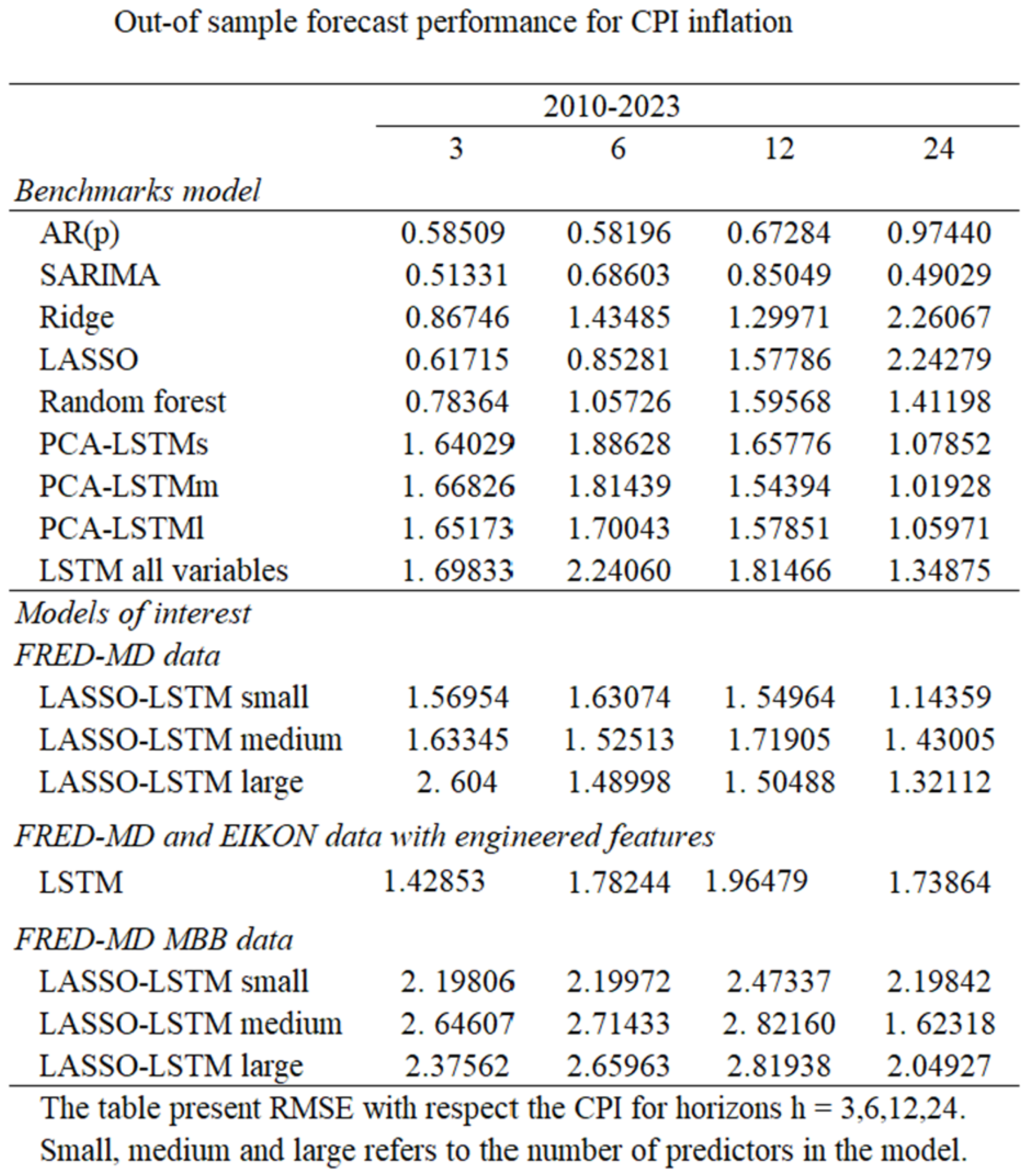
5.2. Benchmark Model Performance

5.2.1. Univariate Models

Both the AR(p) model and the SARIMA model perform well for all forecasting horizons, reaffirming the existing findings in the literature. For very short and very long forecasting horizons, the SARIMA is superior, while for medium long forecasting horizons the AR(p) model is the superior performer. The performance of these naive univariate models is superior to most other models for almost all forecasting horizons.

5.2.2. Machine Learning Models

In our study there are three benchmark machine learning models that are used for comparison with the LSTM model. LASSO is superior compared to other machine learning models on a three month forecasting horizon, and competitive with other models on a 6 month forecast horizon. However as the forecasting horizons increase, the performance of the LASSO model deteriorates showing signs of high bias.

Ridge, the other regularization technique employed in this study, performs similar to LASSO, and achieves good results for short forecast horizons. However, as the horizon increases the performance of the model deteriorates, showing signs of high bias. This suggests that Ridge will adapt to noise in the model and that shrinking coefficients to zero (Lasso) is a better approach when forecasting. LASSO outperforms the Ridge model for all forecasting horizons, except for the 12 month forecast.

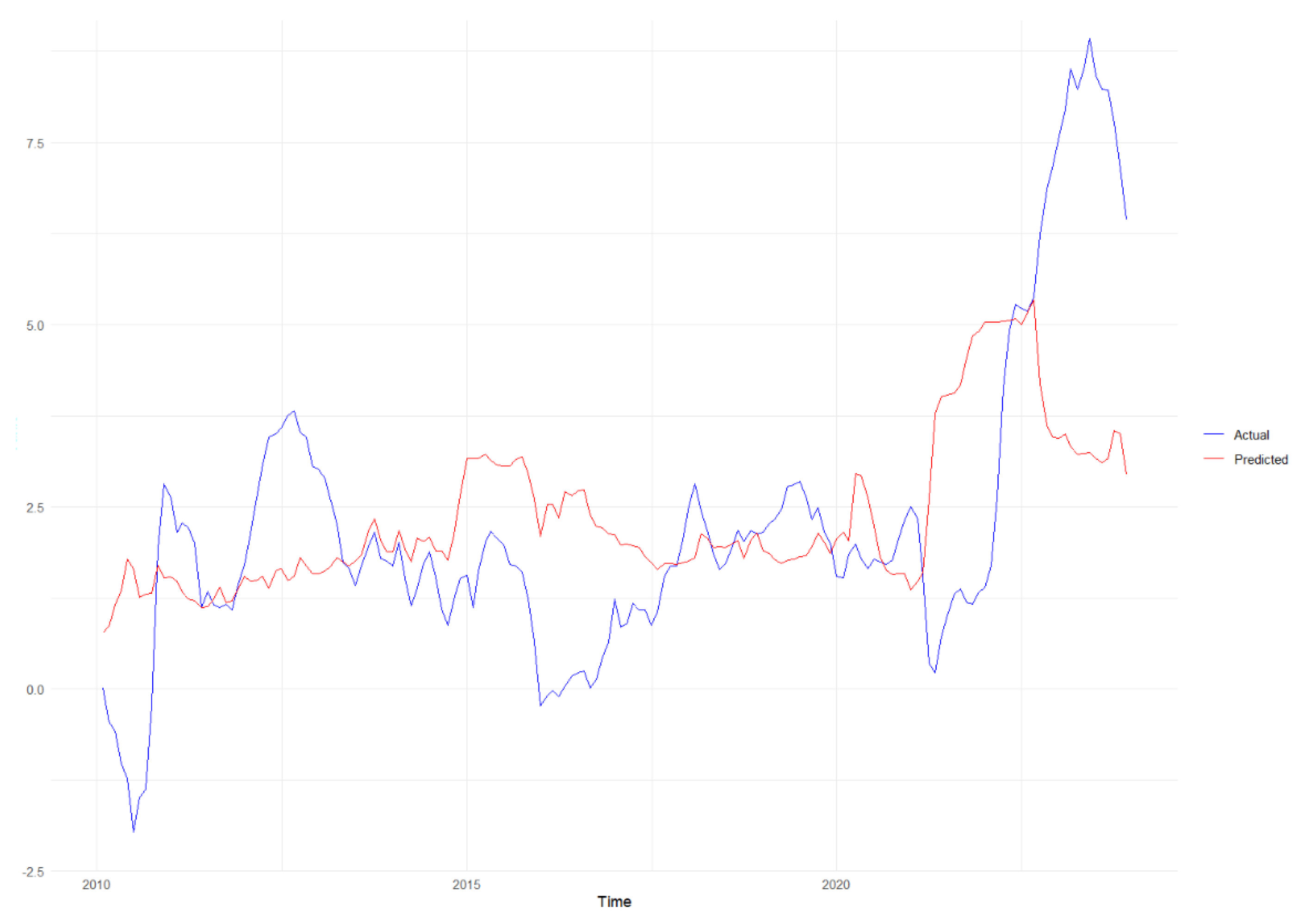
The last machine learning benchmark model is random forest. Figure 5.2 depicts the random forest 12 months inflation forecast against observed inflation over the same time span. Random forest performs worse than LASSO on short forecast horizons, but displays a more consistent performance all over. While LASSO and Ridge perform poorly for the 24 month forecast horizon, random forest produces competitive results.

Figure 10. 12-month forecast using the Random Forest model, comparing actual (blue line) and predicted (red line) values. The model captures general trends but diverges significantly at certain points, particularly towards the end of the forecast period. This indicates some limitations in the model’s predictive accuracy, especially during periods of high volatility.

Figure 10. 12-month forecast using the Random Forest model, comparing actual (blue line) and predicted (red line) values. The model captures general trends but diverges significantly at certain points, particularly towards the end of the forecast period. This indicates some limitations in the model’s predictive accuracy, especially during periods of high volatility.

5.2.3. PCA-LSTM Performance

The LSTM benchmark models are applied with PCA, where feature selection comes in three forms; LSTM small, LSTM medium, LSTM large. For shorter forecast horizons the LSTM models perform poorly compared to the machine learning models and the univariate models. This differs somewhat from findings in the literature, but it is not too surprising since there is not much work on inflation forecasting using LSTM models. Our findings of LSTM on shorter forecasting horizons affirm the need for further studies to determine the ability of neural networks for forecasting inflation. On longer forecasting horizons the LSTM model outperforms other machine learning models, and is partially on par with univariate models. Comparing the three architecture sizes of the LSTM model illustrates that for short to medium forecasting horizons, the differences are negligible.

For longer forecasting horizons the medium sized architecture performs best, which is probably a result of the balance between overfitting and underfitting the model.

5.3. LSTM Model Performance

5.3.1. LASSO-LSTM - FRED-MD Data

The LASSO-LSTM models differ from LSTM in the process of feature selection. Specifically, we examine how LASSO-LSTM performs compared to LSTM applying the standard PCA feature selection approach.

Results show that for small architectures the LASSO-LSTM model is able to perform better than the PCA-LSTM model. This is consistent for all horizons except for 24 months ahead, for which PCA-LSTM is marginally better. For medium and large size architectures there is little difference between the LASSO LSTM and PCA-LSTM. As the number of predictors increases, and gets closer to the total number of available predictors, the two models converge in performance.

Among the different LASSO-LSTM models the smallest architecture is the best performer. It produces superior 3 and 24 month forecasts but it is slightly outperformed on 6 and 12 month forecasts. The medium architecture is quite consistent for all forecasting horizons, but performs worse than the small architecture. The large architecture has some outstanding results, but also some quite poor ones. This is probably due to overfitting. Notably, the large LASSO-LSTM architecture is able to outperform the LSTM model without any feature selection, meaning any feature selection is better than none. Despite some good forecasts from larger architectures, fewer predictors avoiding overfitting are preferable for inflation forecasting.

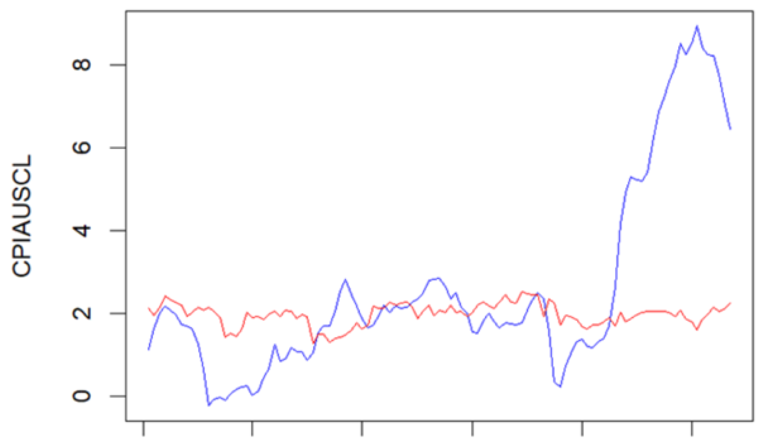
Figure 5.3 illustrates the performance of 6 month inflation forecasts from the LASSO-LSTM model. The model struggles to capture sudden powerful changes in volatility. The observed under-performance during these volatile periods suggests that while the LASSO-LSTM model is robust in stable conditions, it may need further tuning or additional features to improve its predictive accuracy when the regime in the data changes. This highlights a common challenge in time series forecasting, that models often need to be continuously adapted to handle the complexities of real-world data.

Figure 11. This figure illustrates a 6-month forecast using the LASSO-LSTM model, showing actual (blue line) and predicted (red line) CPIAUSCL values. The model closely follows the actual values in periods of low volatility but struggles to capture sharp increases, particularly towards the end of the forecast period. This indicates the model’s limitations in predicting sudden changes in the data.

Figure 11. This figure illustrates a 6-month forecast using the LASSO-LSTM model, showing actual (blue line) and predicted (red line) CPIAUSCL values. The model closely follows the actual values in periods of low volatility but struggles to capture sharp increases, particularly towards the end of the forecast period. This indicates the model’s limitations in predicting sudden changes in the data.

5.3.2. FRED-MD and EIKON Data with Feature Engineering

The reader should recall that a performance summary, in terms of RMSE, is provided in Figure 5.1. The LSTM model with financial data from the EIKON database and FRED-MD primarily utilizes prices, and performs well on the short forecasting horizon but poorly on longer horizons.

This model utilizes prices and not variables reflecting economic activity. As economic activity is important for longer forecasting horizons, it makes sense that this model performs best for shorter forecasting horizons. Of all LSTM models the financial data LSTM is the best performing model on the short forecasting horizons.

5.3.3. FRED-MD - MBB Data

The final set of models has undergone a similar feature selection approach as the first set of LASSO-LSTM and utilize of the same dataset. These models only differ because of the moving block bootstrapping. The most important model for comparison in this case is the LASSO-LSTM with FRED-MD data. The results related to the data augmented LASSO-LSTM model is quite uninspiring, and the model is not able to deliver superior results at any forecasting horizon for any size of architecture. Thus data augmentation as an attempt to increase training data was unsuccessful. The model training time also increases considerably compared to all other LSTM models. Presumably, the augmented data does not retain the sequence well enough, and is ineffective in capturing different regimes and other patterns in macroeconomic data.

5.4. Benchmarks Versus LSTM-Type Models

While seeing an improvement in performance when switching from PCA to LASSO feature selection, LSTM is still not able to deliver competitive forecasts compared to the univariate time series models. For shorter forecasting horizons there are other machine learning models, such as LASSO, that are able to provide better forecasts than LSTM. Random forest is also better at shorter forecast horizons. As forecast horizons increase, LSTM forecasts improve. The LSTM model is better than all of the machine learning models for the 24 month forecast, and quite good for 12 month forecasts. All other machine learning models show signs of high bias in their 24 months forecasts. However, this issue was not possible to solve during specification on the validation sample, as LASSO and random forest did not improve when features were removed or added. This indicates that the LSTM model could be a good option compared to other machine learning models on longer forecast horizons.

5.5. Limitations of Our Research

5.5.1. Data Constrains

A primary limitation in applying Long Short-Term Memory (LSTM) models to macroeconomic forecasting is the scarcity and quality of available data. LSTM networks are data-intensive, requiring substantial datasets to effectively learn temporal patterns. However, macroeconomic indicators are typically reported at monthly or quarterly intervals, resulting in relatively small datasets. Moreover, data quality prior to 1960 is often inconsistent, further constraining the training process.

Additionally, the relationship between inflation and its predictors is inherently complex and non-linear. While LSTM models are adept at capturing non-linear patterns, they assume a degree of stationarity in these relationships. In practice, macroeconomic relationships are subject to structural changes over time, leading to non-stationarity that can challenge the model’s predictive capabilities. Recent studies have highlighted that while LSTM models can outperform traditional models in certain contexts, their performance may degrade when faced with such non-stationary data patterns .

5.5.2. Forecast Horizon and Model Complexity

Our findings indicate that LSTM models tend to perform better over longer forecasting horizons, particularly during periods of heightened macroeconomic uncertainty. This aligns with recent research suggesting that LSTM models can capture long-term dependencies more effectively than some traditional models. However, for shorter horizons, simpler models like LASSO regression or SARIMA often yield more accurate forecasts. This inconsistency complicates the recommendation of LSTM models for general forecasting purposes.

Furthermore, LSTM architectures involve numerous layers and hyperparameters, making them complex to configure and tune. This complexity not only increases the computational burden but also poses challenges for reproducibility and interpretability—key considerations for policymakers and practitioners. The “black-box” nature of LSTM models can hinder the extraction of actionable insights, a limitation that has been noted in the context of economic forecasting.

By acknowledging these limitations, future research can focus on hybrid approaches that combine the strengths of LSTM models with the interpretability of traditional methods, or explore alternative architectures better suited to the nuances of macroeconomic data.

5.6. Future Research

To enhance the accuracy of inflation forecasting models, future research should focus on advanced data augmentation techniques that preserve the inherent properties of time series data, such as regime shifts and random walk characteristics. Implementing methods like Moving Block Bootstrapping (MBB) can help maintain autocorrelation structures within the data, leading to more robust model training. Integrating LASSO regularization into Long Short-Term Memory (LSTM) networks has shown promise in improving model performance by effectively handling high-dimensional datasets and preventing overfitting. Additionally, exploring ensemble approaches that combine LASSO with tree-based models, such as Random Forests, can leverage the strengths of both methods to capture complex patterns in inflation data.

While ensemble models offer potential performance gains, it’s important to consider the balance between model complexity and interpretability. Tree-based models and penalized regression techniques, like LASSO, often provide more transparent insights, which are valuable for policymakers. Although current LSTM models may underperform compared to simpler alternatives, advancements in recurrent neural networks (RNNs) could enhance their applicability in macroeconomic forecasting.

Furthermore, investigating other neural network architectures, such as Convolutional Neural Networks (CNNs) and Transformers, may yield valuable insights due to their ability to capture both local and global dependencies in time series data.

6. Conclusions

This study evaluated the effectiveness of Long Short-Term Memory (LSTM) models in forecasting U.S. inflation, comparing their performance against traditional time series models such as SARIMA and AR(p), as well as machine learning approaches like LASSO regression. While integrating LASSO for feature selection enhanced LSTM performance, the LSTM models generally underperformed compared to simpler models across most forecasting horizons.

Notably, LSTM models showed relative strength in longer-term forecasts. However, their complex architecture, which includes numerous layers and hyperparameters, poses challenges in model tuning and reproducibility. Additionally, the “black box” nature of LSTM models limits interpretability, a crucial factor for policymakers and central bankers who require transparent and explainable forecasting tools.

Data limitations may contribute to the subpar performance of LSTM models in this context. Macroeconomic data, such as inflation indicators, are typically reported at monthly or quarterly intervals, resulting in relatively small datasets. Furthermore, the data encompasses unique economic events—including shifts in central bank policies, the Global Financial Crisis, and the COVID-19 pandemic—which introduce complex, non-stationary relationships that are challenging for LSTM models to capture effectively.

While LSTM models are capable of modeling non-linear patterns, their performance is hindered when these non-linearities evolve over time. In contrast, simpler models like LASSO regression, AR(p), and SARIMA have demonstrated more consistent and reliable performance in inflation forecasting, making them more suitable for practical applications in economic policy and decision-making.

Future research should explore advanced data augmentation techniques, such as Moving Block Bootstrapping (MBB), to enhance LSTM model training and mitigate overfitting. Additionally, hybrid models that combine the strengths of LSTM networks with traditional time series approaches may offer improved forecasting accuracy. For instance, integrating LSTM with SARIMA has shown promise in capturing both linear and non-linear patterns in inflation data.

In terms of interpretability, incorporating LASSO for feature selection within LSTM models (LASSO-LSTM) has provided clearer insights into variable importance, as LASSO emphasizes significant predictors while diminishing the influence of less relevant ones. This approach not only enhances model transparency but also contributes to improved forecasting accuracy, as evidenced by lower Root Mean Square Error (RMSE) values.

In conclusion, while LSTM models offer potential advantages in modeling complex, non-linear relationships, their current limitations, particularly in data-scarce environments—suggest that simpler, more interpretable models like LASSO regression, AR(p), and SARIMA remain more practical and effective for inflation forecasting. Advancements in data augmentation and hybrid modeling approaches may, however, enhance the applicability of LSTM models in future macroeconomic forecasting endeavors.

References

- Almosova, A., & Andresen, N. 2023. Nonlinear inflation forecasting with recurrent neural networks. Journal of Forecasting422240-259.
- Atkeson, A., Ohanian, L. E., et al. 2001. Are Phillips curves useful for forecasting inflation? Federal Reserve bank of Minneapolis quarterly review2512–11.
- Bishop, C. M. 2006. Pattern recognition and machine learning. Springer google schola21122–1128.
- Chen, Y.-c., Turnovsky, S. J., & Zivot, E. 2014. Forecasting inflation using commodity price aggregates. Journal of Econometrics1831117–134.
- Dubey, A. K., Kumar, A., García-Díaz, V., Sharma, A. K., & Kanhaiya, K. 2021. Study and analysis of SARIMA and LSTM in forecasting time series data. Sustainable Energy Technologies and Assessments47101474.
- Fisher, J. D., Liu, C. T., & Zhou, R. 2002. When can we forecast inflation? Economic Perspectives-Federal Reserve Bank of Chicago26132–44.
- Forni, M., Hallin, M., Lippi, M., & Reichlin, L. 2003. Do financial variables help forecasting inflation and real activity in the euro area? Journal of Monetary Economics5061243–1255.
- Freijeiro-González, L., Febrero-Bande, M., & González-Manteiga, W. 2022. A critical review of LASSO and its derivatives for variable selection under dependence among covariates. International Statistical Review901118–145.
- Garcia, M. G., Medeiros, M. C., & Vasconcelos, G. F. 2017. Real-time inflation forecasting with high-dimensional models: The case of Brazil. International Journal of Forecasting333679–693.
- Groen, J. J., Paap, R., & Ravazzolo, F. 2013. Real-time inflation forecasting in a changing world. Journal of Business & Economic Statistics31129–44.
- Iversen, J., Laséen, S., Lundvall, H., & Soderstrom, U. 2016. Real-time forecasting for monetary policy analysis: The case of Sveriges Riksbank. Riksbank Research Paper Series142.
- Lenza, M., Moutachaker, I., & Paredes, J. 2023. Forecasting euro area inflation with machine-learning models. Research Bulletin112.
- Meyler, A., Kenny, G., & Quinn, T. 1998. Forecasting Irish inflation using ARIMA models.
- Mullainathan, S., & Spiess, J. 2017. Machine learning: an applied econometric approach. Journal of Economic Perspectives31287–106.
- Paranhos, L. 2024. Predicting Inflation with Recurrent Neural Networks. Journal of Economic Forecasting584567-589.
- Ranstam, J., & Cook, J. A. 2018. LASSO regression. Journal of British Surgery105101348–1348.
- Robinson, W. 1998. Forecasting inflation using VAR analysis. Econometric Modelling of Issues in Caribbean Economics and Finance. CCMS: St. Augustine, Trinidad and Tobago.
- Staiger, D., Stock, J. H., & Watson, M. W. 1997. The NAIRU, unemployment and monetary policy. Journal of economic perspectives11133–49.
- Stock, J. H., & Watson, M. W. 2003. Forecasting output and inflation: The role of asset prices. Journal of economic literature413788–829.
- Stock, J. H., & Watson, M. W. 2008September. Phillips Curve Inflation Forecasts Phillips curve inflation forecasts Working Paper No. 14322. National Bureau of Economic Research.
- Theoharidis, A. F., Guillén, D. A., & Lopes, H. 2023. Deep learning models for inflation forecasting. Applied Stochastic Models in Business and Industry393447–470.
- Tibshirani, R. 1996. Regression shrinkage and selection via the lasso. Journal of the Royal Statistical Society Series B: Statistical Methodology581267–288.
- Tsui, A. K., Xu, C. Y., & Zhang, Z. 2018. Macroeconomic forecasting with mixed data sampling frequencies: Evidence from a small open economy. Journal of Forecasting376666–675.
Disclaimer/Publisher’s Note: The statements, opinions and data contained in all publications are solely those of the individual author(s) and contributor(s) and not of MDPI and/or the editor(s). MDPI and/or the editor(s) disclaim responsibility for any injury to people or property resulting from any ideas, methods, instructions or products referred to in the content. |
© 2025 by the authors. Licensee MDPI, Basel, Switzerland. This article is an open access article distributed under the terms and conditions of the Creative Commons Attribution (CC BY) license (http://creativecommons.org/licenses/by/4.0/).
Copyright: This open access article is published under a Creative Commons CC BY 4.0 license, which permit the free download, distribution, and reuse, provided that the author and preprint are cited in any reuse.