1. Introduction
The study of phase transitions is one of the most important tasks in theory, in experiments and in computer simulations since the second half of the 20th century. The main reason is that, if we know the characteristics of a phase transition, we can understand the interaction mechanisms lying behind the transition and we can deduce various physical quantities. Therefore, comparisons between theories, experiments and computer simulattions are necessary in order to obtain conclusions. While comparison with experments is always a challenge because real materials may contain ill-controlled elements such as dislocations, defects and impurities, comparisons between theories and simulations are in most cases possible. This is the purpose of the present short review based on our own works in the past years.
Let us recall that the phase transition was first studied by the mean-field approximation with several improved versions in the 40s (see the textbook [
1] where these methods are shown and commented). These were followed by exact-solution methods in two dimensions (2D) such as the Ising model, Potts models and vertex models (see the book by R. Baxter [
2]). The break-through in general dimensions come in 1970 with the formulation of the renormalization group by K. G. Wilson [
3,
4] followed by investigations on the finite-size scaling analysis and their validity [
5]. The present Special Issue (SI) revisits the progress made on the scaling and hyperscaling relations above the upper critical dimension
. Several papers in this SI recall the foundation of these relations in a general
d. The reader is referred, for example, to the review by A. Peter Young [
6] for a recall of the demonstration of these relations (see also the review by Honchar et al. [
7]). The main question of this SI is whether or not the hyperscaling is violated for dimension
d larger than the upper critical dimension
. However, we show that the question of the violation of the hyperscaling is also posed in
in some specific cases that we will present in this paper.
The first case concerns the critical exponents obtained by using the highly-precise multi-histogram Monte Carlo (MC) technique [
8,
9,
10] for a thin film of simple cubic structure with Ising spin model. The film surface
(
plane) is very large, up to
lattice sites for some cases, with periodic boundary conditions, while the film thickness
goes from one layer (2D) to 13 layers with free boundary conditions. Finite-size scaling (FSS) has been used with varying
L to calculate the critical exponents. These results have been published in Ref. [
11] but the aspect of the violation of the hyperscaling relation has not been discussed. In the light of the topic of the present Special Issue, we revise the interpretation of our results. In addition, we review some other cases that we have investigated.
Except the case
, the question on the dimension of the system is naturally arised. For Capehart and Fisher [
12], there is a cross-over from 2D to 3D when
is increased. So, how to use the hyperscaling relation, namely with which dimension ? We will discuss in this paper.
This short review is organized as follows.
Section 2 is devoted to the case of thin films mentioned above where the multi-histogram technique is recalled.
Section 3 shows the results of critical exponents obtained with the FSS.
Section 4 reviews the case of a cross-over between the first- and second-order transitions when the film thickness is decreased.
Section 5 is devoted to some other cases where the hyperscaling relation is violated or seems to be violated. Concluding remarks are given in
Section 6.
3. Results
Most of the results shown below have been published by us in [
11]. However, in light of the new interpretation on the violation of the hyperscaling relation, we review them here to show that there is a possibility that the hyperscaling relatrion
is violated below
: as said in the Introduction, in the case of thin films where the thickness is finite and small, the hyperscaling relation is satisfied only when
d has a value between 2 and 3. This non-integer dimension is called by Capehart and Fisher [
12] "cross-over dimension". To our knowledge,
d in the hyperscaling relation is the space dimension, it is 2, 3, ... (integer), it cannot be between 2 and 3. We are convinced that the hyperscaling relation may not be valid in the case of thin films shown below and in other particular cases shown in
Section 5.
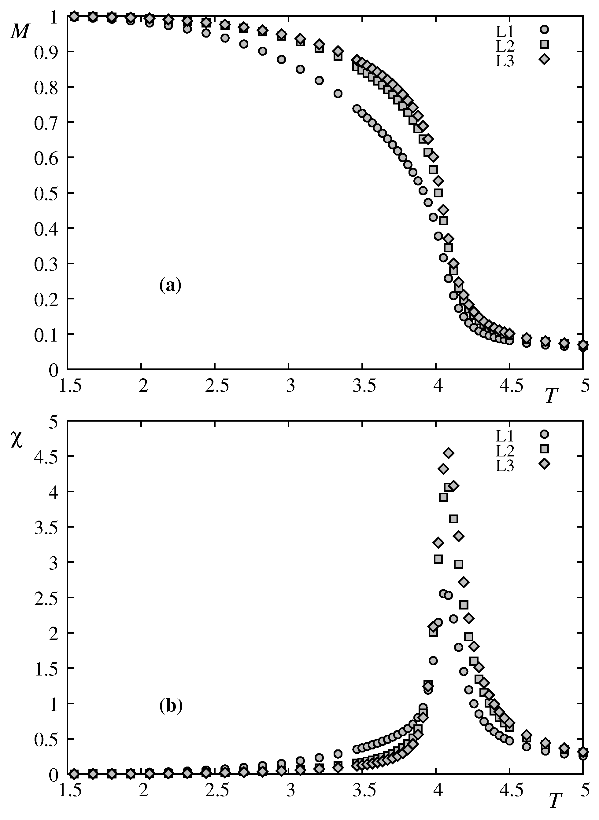
First, we show the layer magnetizations and their corresponding susceptibilities of the first three layers in the case where
in
Figure 1. The layer susceptibilities have their peaks at the same temperature, indicating a single transition. We note that the magnetization is lowest at the surface and increases while going to the interior. This is known a long time ago by the Green’s function method [
15,
16] and by more recent works on thin films with competing interactions [
17] and films with Dzyaloshinskii-Moriya interaction [
18,
19]. Physically, the surface spins have smaller local field due to the lack of neighbors, so thermal fluctuations will reduce more easily the surface magnetization with respect to the interior ones.
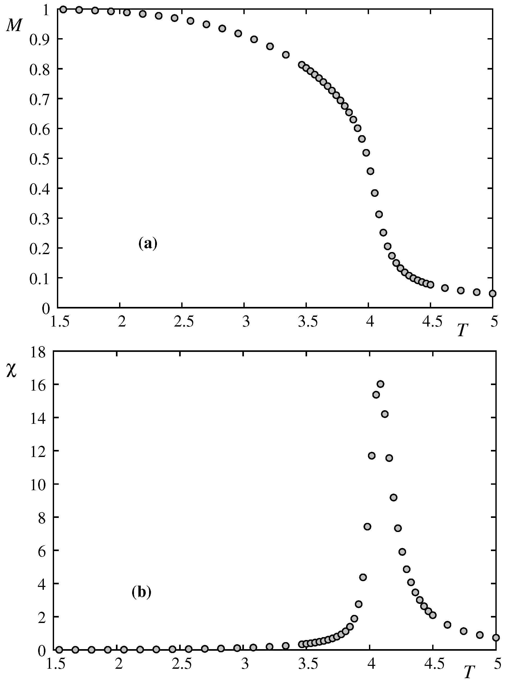
We plot in
Figure 2 the total magnetization and the total susceptibility. The latter shows only one peak, signature of a single transition. This justifies the study shown below on the criticality of the film transition.
3.1. Finite Size Scaling
Let us show our finite-size scaling (FSS) with L varying from 20 to 80. For we use L up to 160 to evaluate the corrections to scaling.
The technical details can be seen in [
11]. We just summarize here: for a given
we use first the standard MC simulations to determine for each size the peak temperatures
of
and
of
. The equilibrating time is from 200000 to 400000 MC steps/spin and the averaging time is from 500000 to 1000000 MC steps/spin. Next, as said earlier, we record the energy histograms at 8 different temperatures
around the transition temperatures
and
with 2 millions MC steps/spin, after discarding 1 millions MC steps/spin for equilibrating. Such an iteration procedure gives extremely good results. Errors shown in the following have been estimated using statistical errors, which are very small thanks to our multiple histogram procedure, and fitting errors given by fitting software.
3.2. Critical Exponents Obtained with Finite-Size Scaling
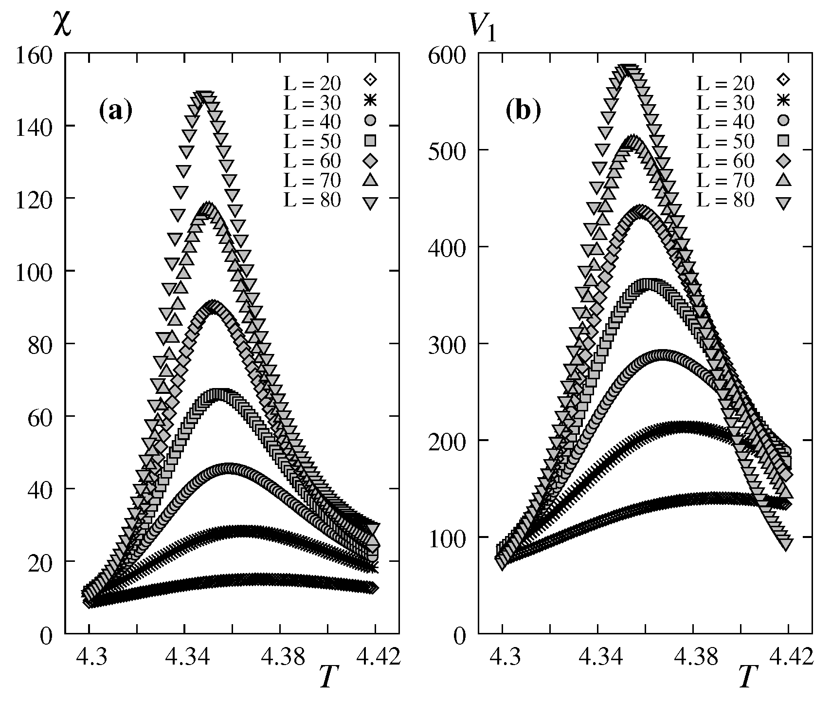
We show first the peak height of the susceptibility and the maximum of
as functions of
T for varying
L from 20 to 80 in
Figure 3.
Note that the results shown below are obtained using
as said earlier below Eq. (
13).
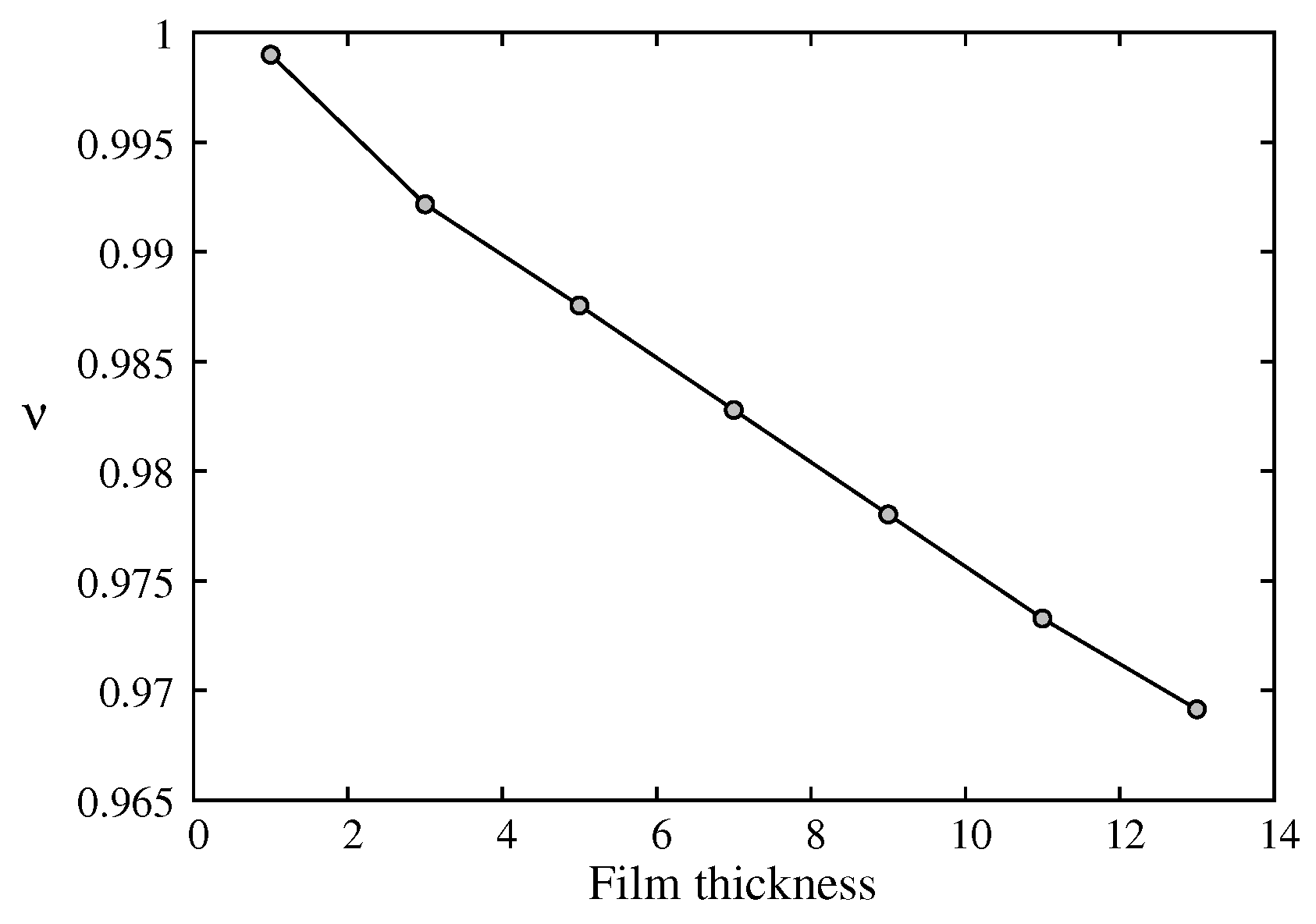
Exponent
is shown as a function of
in
Figure 5
To show the precision of our method, we give here the results of
. For
, we have
which yields
and
and
. These results are in excellent agreement with the exact results
and
. The very high precision of our method is thus verified in the rather modest range of the system sizes
used in the present work. Note that the result of Ref.[
20] gave
for
which is very far from the exact value.
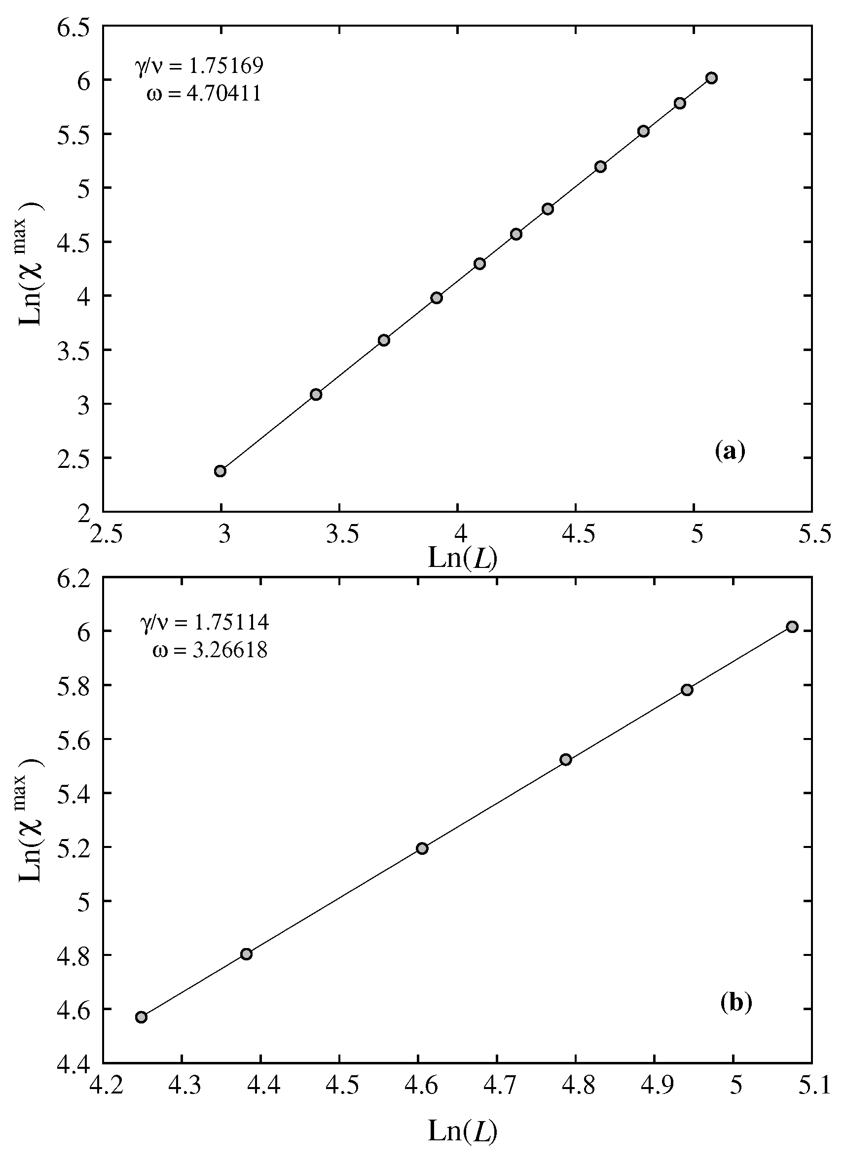
3.3. Corrections to Scaling
Let us touch upon the question of corrections to scaling said earlier. We show now that the corrections to scaling are very small.
We consider here the effects of larger
L and of the correction to scaling for
. The results indicate that larger
L does not change the results shown above.
Figure 9(a) displays the maximum of
as a function of
L up to 160. Using Eq. (
8), i. e. without correction to scaling, we obtain
which is to be compared to
using
L up to 80. The change is therefore insignificant because it is at the third decimal i. e. at the error level. The same is observed for
as shown in
Figure 9(b):
using
L up to 160 instead of
using
L up to 80.
Now, let us allow for correction to scaling, i. e. we use Eq.(
14) instead of Eq. (
10) for fitting. We obtain the following values:
,
,
,
if we use
L = 70 to 160 (see
Figure 10). The value of
in the case of no scaling correction is
. Therefore, we can conclude that this correction is insignificant. The large value of
explains the smallness of the correction.
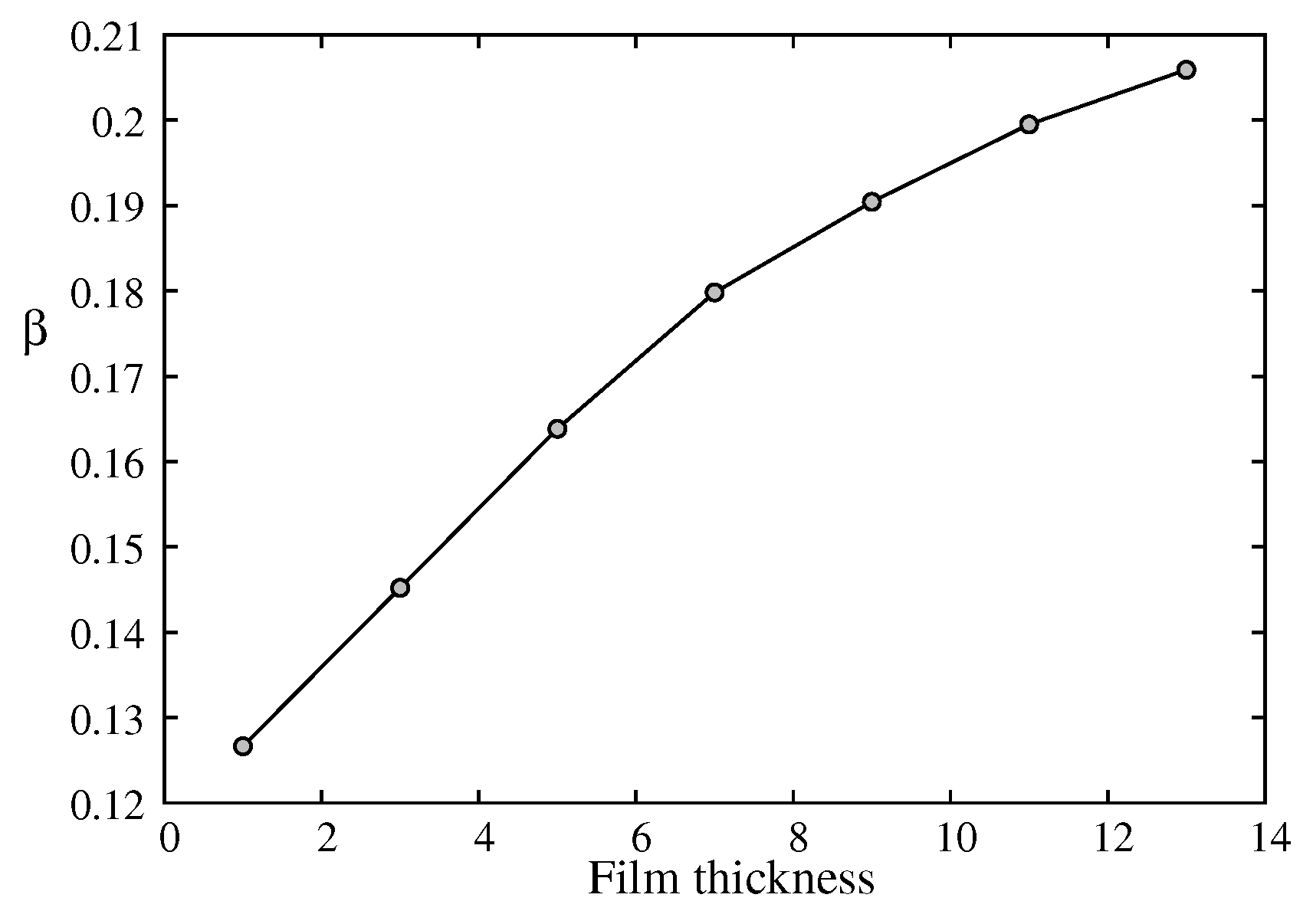
For
, using Eq. (
12) we calculate
for each thickness
. The results are precise. For example for
=1, we obtained
which yields
which is in agreement within errors with the exact result
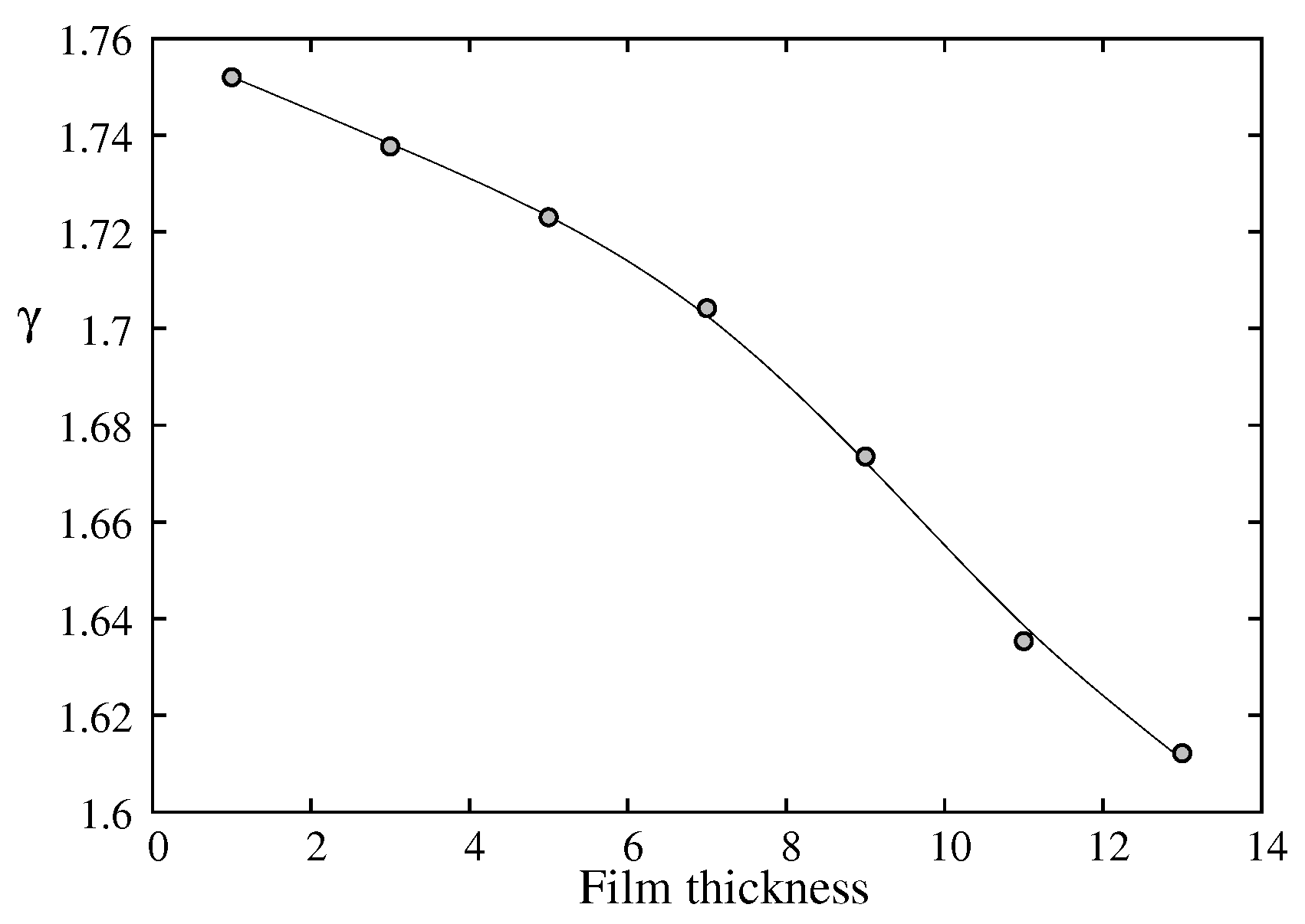
. We show in
Figure 11 the exponent
versus
.
3.4. Summary of Our Results
We summarize our results in
Table 1. Note that if we use
and
for a given
, except the case
, the hyperscaling relation
is violated if
. This relation is obeyed if the dimension is replaced by an "effective dimension"
listed in
Table 1 which is larger than 2. The last column shows the critical temperature at
obtained by using Eq. (
13).
3.5. Discussion
Let us show in
Figure 12 the effective dimension versus
. As seen, though
deviates systematically from
, its values are however very close to 2. This means that the 2D character is dominant even at
.
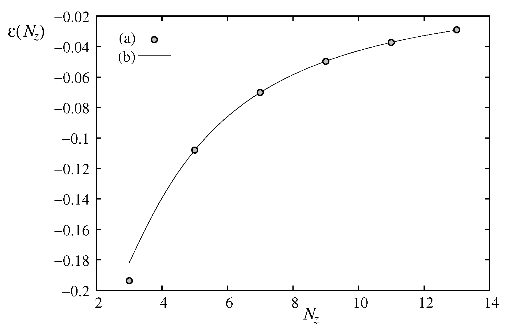
As mentioned above,
is very close to 2. However,
increases very fast to reach a value close to
of the 3D Ising model (
) at
. This is an interesting point. In Ref. [
12] Capehart and Fisher define the critical-point shift as
They showed that
where
(3D value). Using
, we fit the above formula with
taken from
Table 1, we obtain
and
.
Our results and the fitted curve are shown in
Figure 13. Note that the correction factor
is necessary to obtain a good fit for small
. The prediction of Capehart and Fisher is verified by our result.
If the cross-over dimension raised by Capehart and Fisher [
12] is identified with the effective dimension between 2 and 3, then the hyperscaling relation involving the space dimension
d cannot be satisfied in the case of thin films. Let us take the case
, we have
, while
far from the
value. The hyperscaling relation is thus violated.
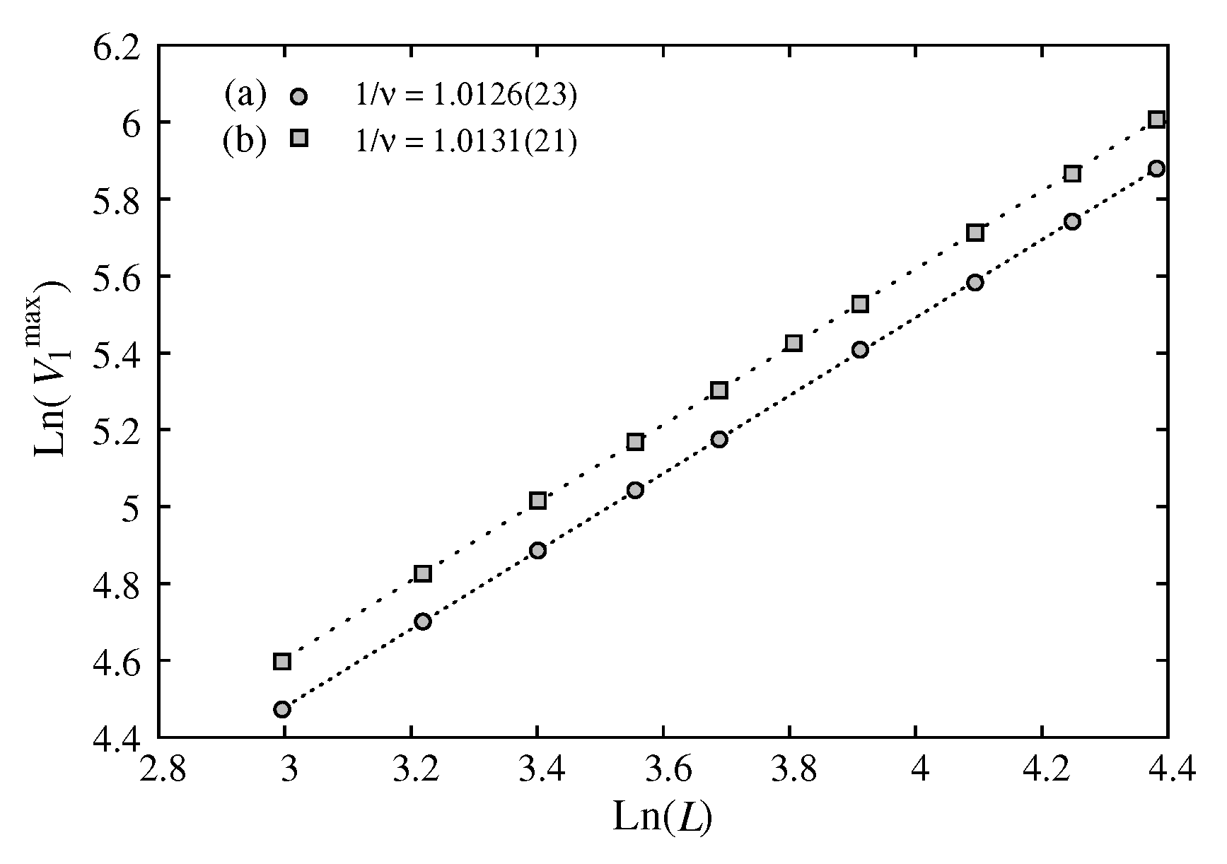
We show now that the free boundary condition in the
z direction gives the same result, within errors, as the periodic boundary condition (PBC), as far as the critical exponents are concerned. This is shown in
Figure 14 and
Figure 15.
We would like to emphasize that the Rushbrooke inequality
is verified within errors as an equality for each
as seen in
Table 1.
4. Cross-Over from First- to Second-Order Transition with Varying Film Thickness
In this section, we show that the film thickness can alter the nature of the transition. We cite here our work on the cross-over between the first- and second-order transition when the film thickness of a fully frustrated FCC antiferromagnet with Ising spins is decreased to
layers (two FCC cells). We used the highly-efficient Wang-Landau method [
21,
22,
23,
24,
25,
26,
27] to detect the thickness where the first-order transition becomes of second-order.
Figure 16 shows the strong first-order character of the transition with an energy discontinuity in the bulk case.
In the case of a thin film composed of 8 layers (
=4 FCC cells in the
z direction), the first-order character remains as shown in
Figure 17 with a double-peak structure.
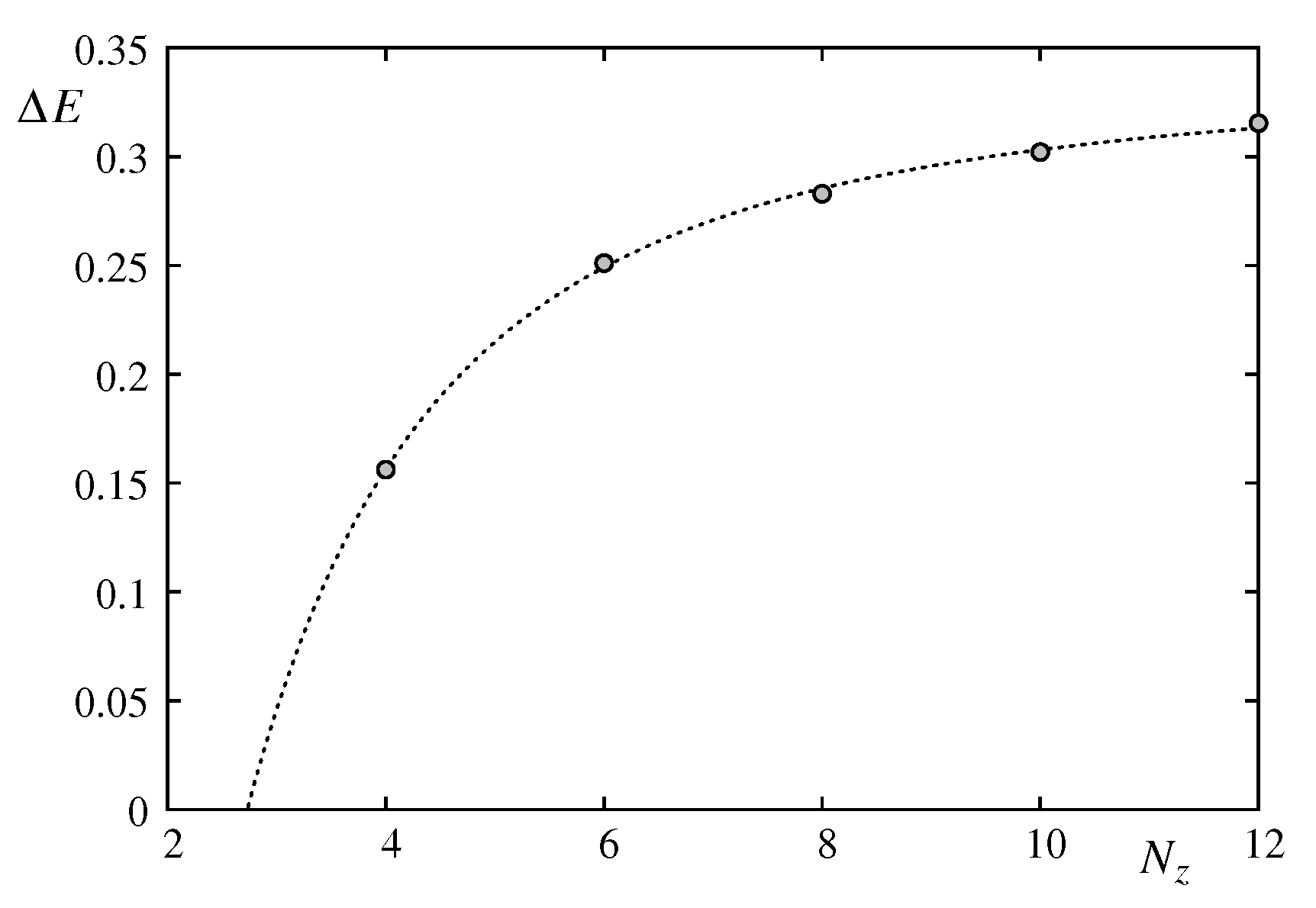
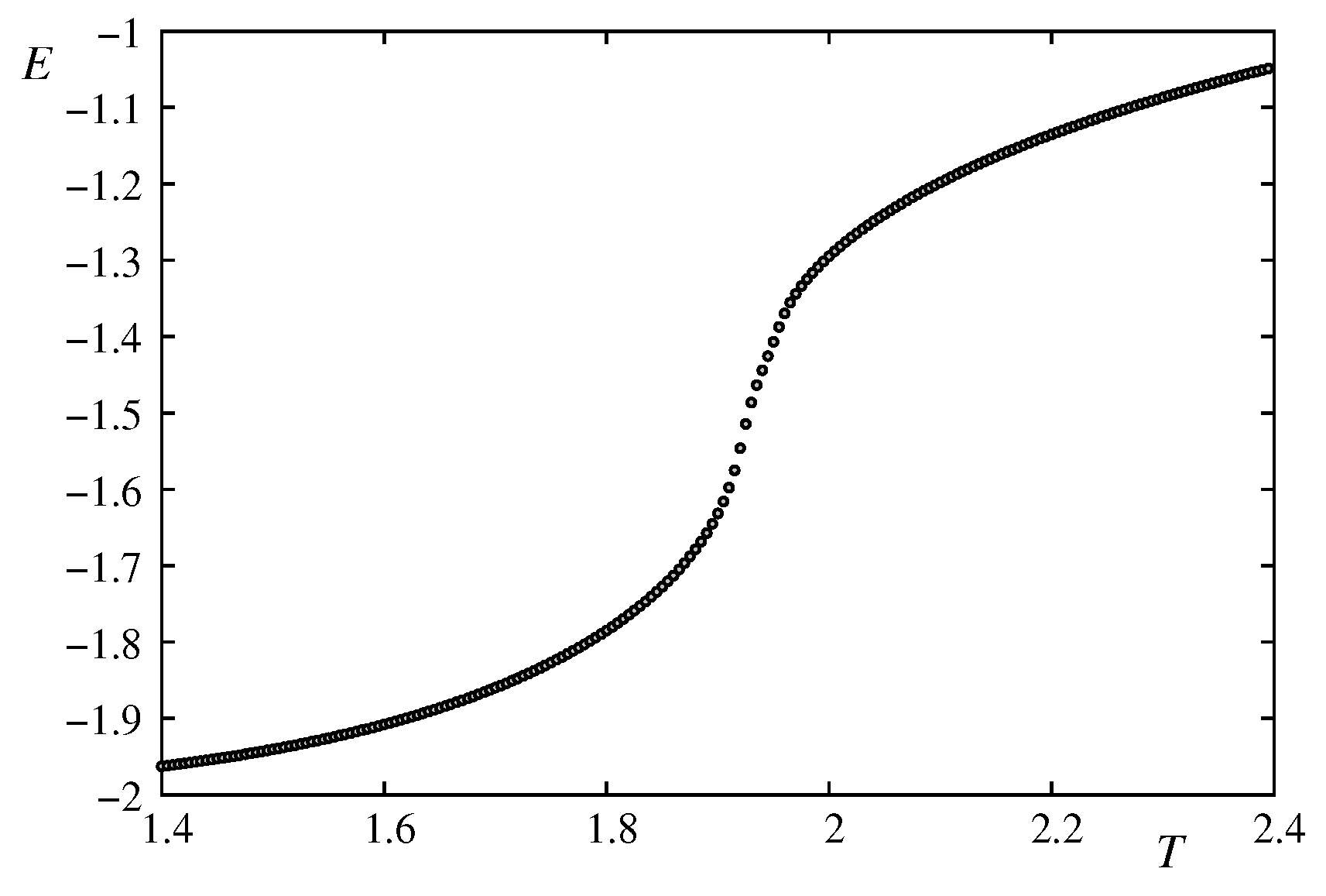
When we decrease the film thickness, the latent heat goes to zero at 4 layers (i. e.
) as shown in
Figure 18.
We have fitted
with the following function
where
is the space dimension,
. The second term in the brackets corresponds to a size correction. As seen in
Figure 18, the latent heat vanishes at a thickness
. This is verified by our simulations for a 4-layer film: the transition has a continuous energy across the transition region, even when
.
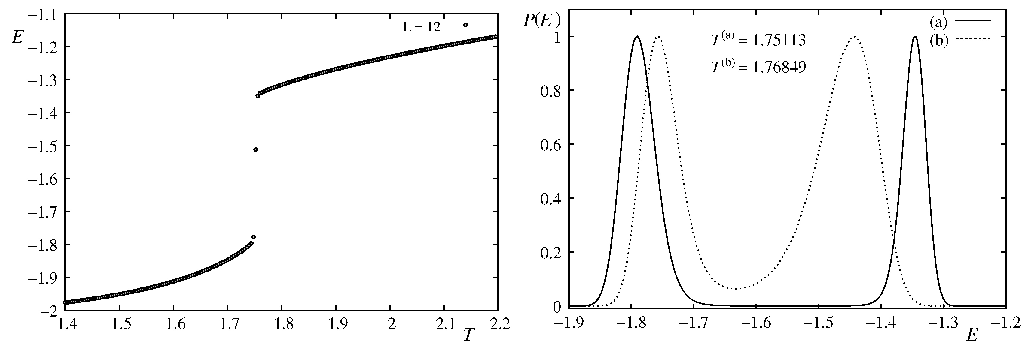
The energy versus
T for
is shown in
Figure 19.
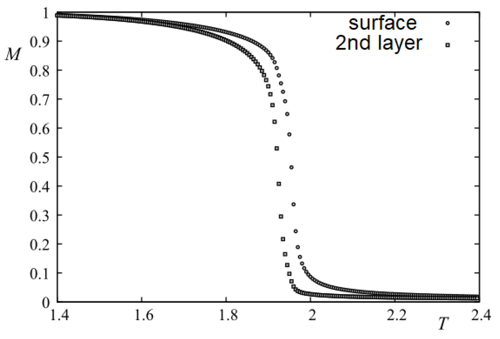
As seen in
Figure 20, there are two close transitions: transition of the surface layers at
and
, and that of the beneath layers at
and
(the lattice constant is taken to be 1).
The surface layer has larger magnetization than that of the second layer unlike the non-frustrated case shown in the previous section. One can explain this by noting that due to the lack of neighbors, surface spins are less frustrated than the interior spins, making them more stable than the interior spins. This has been found at the surface of the frustrated helimagnetic film [
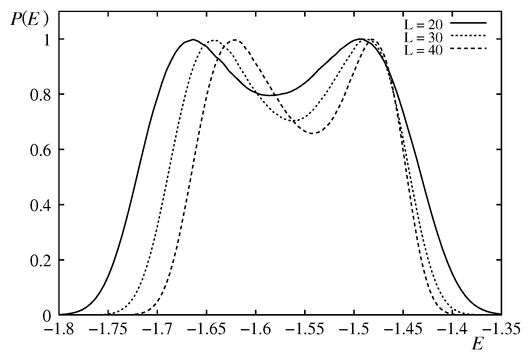
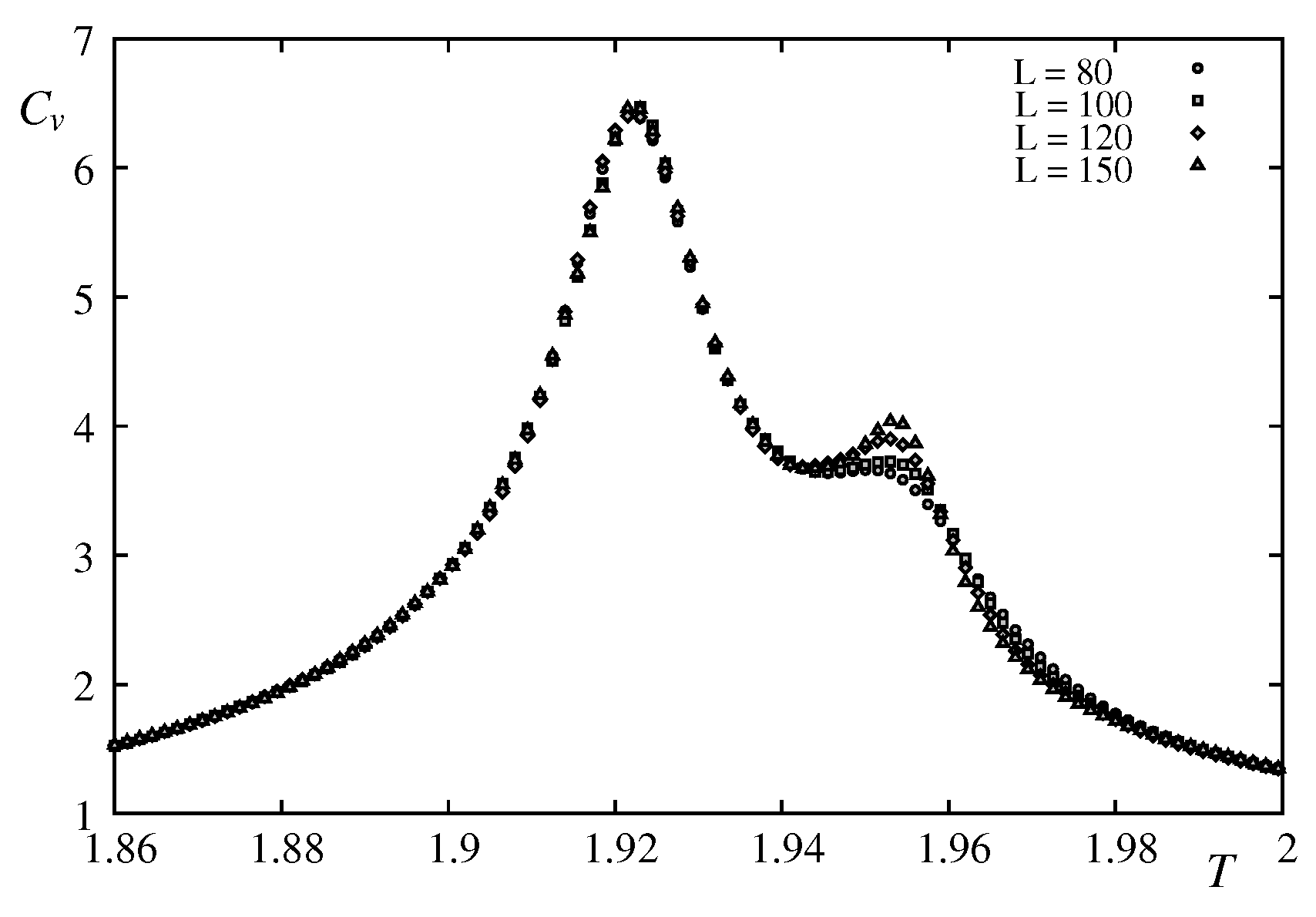
17]. In order to find the nature of these transitions, using the Wang-Landau technique we study the finite-size effects which are shown in in
Figure 21 and
Figure 22. The first peak at
corresponds to the vanishing of the second-layer magnetization, it does not depend on the lattice size, while the second peak at
, corresponding to the disordering of the two surface layers, it depends on
L. The histograms shown in
Figure 23 are taken at and near the transition temperatures show a Gaussian distribution indicating a non first-order transition.
The fact that the peak at
of the specific heat does not depend on
L suggests two scenarios: i)
does not correspond to a transition, ii)
is a Kosterlitz-Thouless transition. We are interested here to the size-dependent transition at
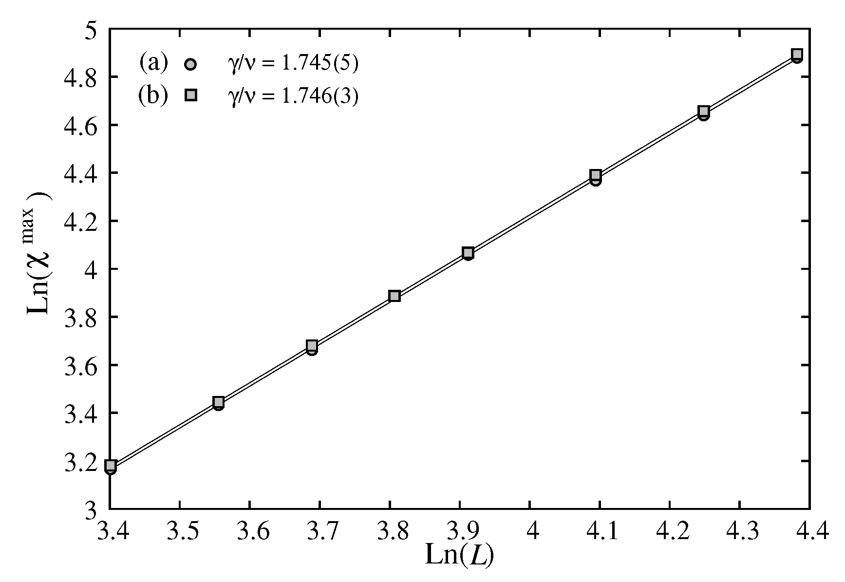
. Using the multi-histogram technique, we have obtained
and
for the case of 4 layers (see
Figure 24 and
Figure 25). These values do not correspond neither to 2D nor 3D Ising models
,
,
,
. We can interpret this as a dimension cross-over between
and
. Note that the values we have obtained
and
belong to a new, unknown universality class.
At the time of our work [
28], we relied on the hyperscaling relation with
to deduce critical exponent
and using the Rushbrooke equality to calculate
. However, in view of a possible violation of the hyperscaling when
d is not the space dimension, we cannot conclude without a direct calculation of
as we have done in the previous section.
6. Concluding Remarks
We know that the hyperscaling relation is verified in
for Ising, XY and Heisenberg spins (results of highly-efficient simulations), and in
for Ising spins (exact results). However, as shown in this review, there are particular cases that the hyperscaling relation
is violated. One of these situations is the case of a magnetic thin film with small thickness. Another case is the fully frustrated XY square lattice where we show that there is a single phase transition of a new coupled XY-Ising universality: the results of Ref. [
35] and our results using the same method of simulation (multiple-histogram technique) are the same for
and
. We did not calculated
, but we believe we should obtain the same
obtained in Ref. [
35] in view of the same results obtained for
and
. The hyperscaling relation is then violated in this case. The case of a system with a magneto-elastic interaction shows a new universality class. The violation, or not, of the hyperscaling relation in this case needs further verifications.
To conclude, let us emphasize that, in view of the precise values we have obtained, at least for thin films, the hyperscaling relation is not verified. We have also presented evidence of the violation of the hyperscaling relation in some other cases. We believe that more cases should be studied before a general conclusion could be drawn. This explains the question mark in the title of this review.
Figure 1.
(a) Layer magnetizations of layer 1 (), layer 2 () and layer 3 () (b) Layer susceptibilities, as functions of T with and .
Figure 1.
(a) Layer magnetizations of layer 1 (), layer 2 () and layer 3 () (b) Layer susceptibilities, as functions of T with and .
Figure 2.
(a) Total magnetization, (b) Total susceptibility, versus T with and .
Figure 2.
(a) Total magnetization, (b) Total susceptibility, versus T with and .
Figure 3.
(a) Susceptibility and (b) , as functions of T for with , obtained by multiple histogram technique.
Figure 3.
(a) Susceptibility and (b) , as functions of T for with , obtained by multiple histogram technique.
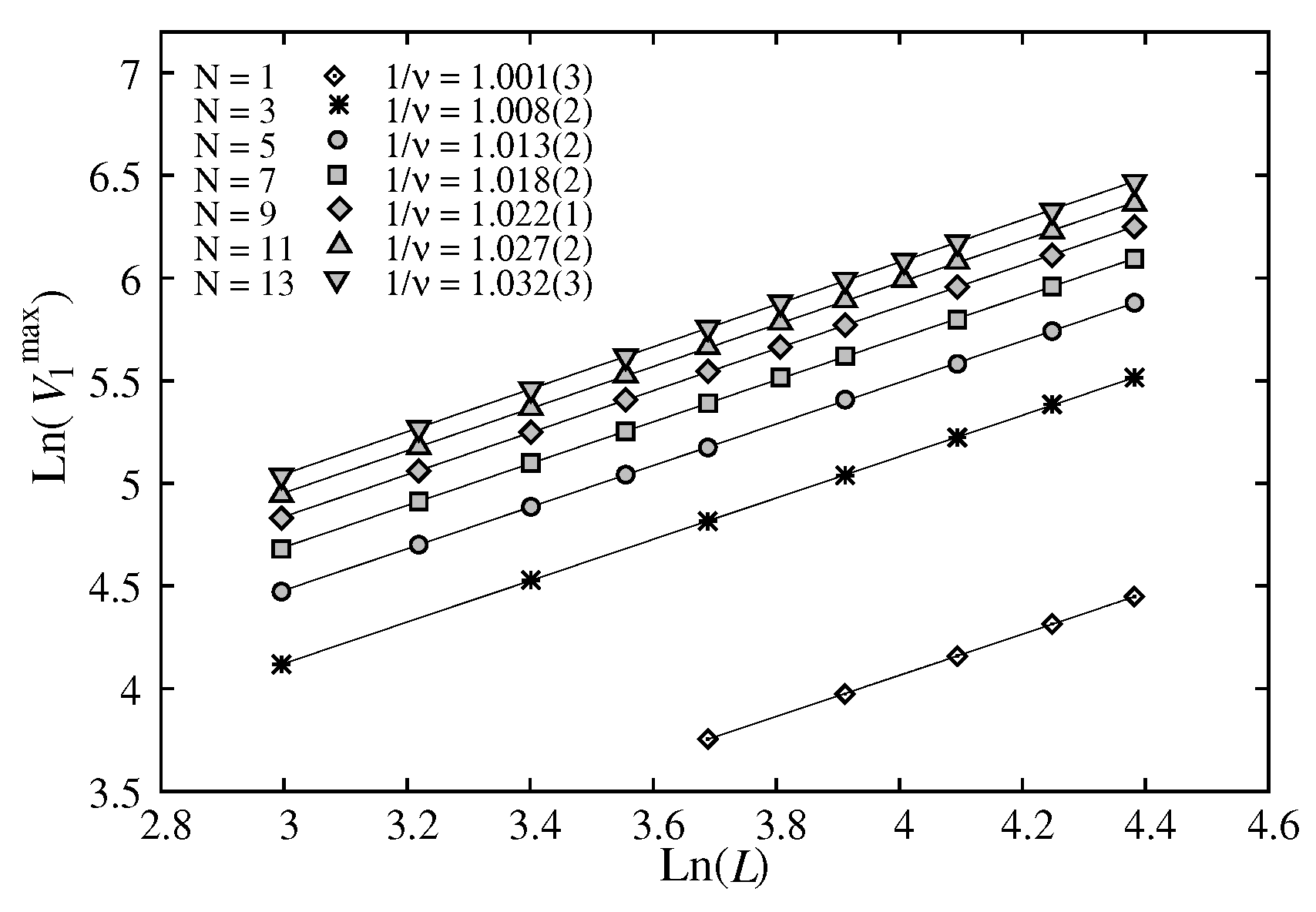
Figure 4.
Maximum of versus L in the scale. The slopes are indicated on the figure.
Figure 4.
Maximum of versus L in the scale. The slopes are indicated on the figure.
Figure 5.
Exponent versus .
Figure 5.
Exponent versus .
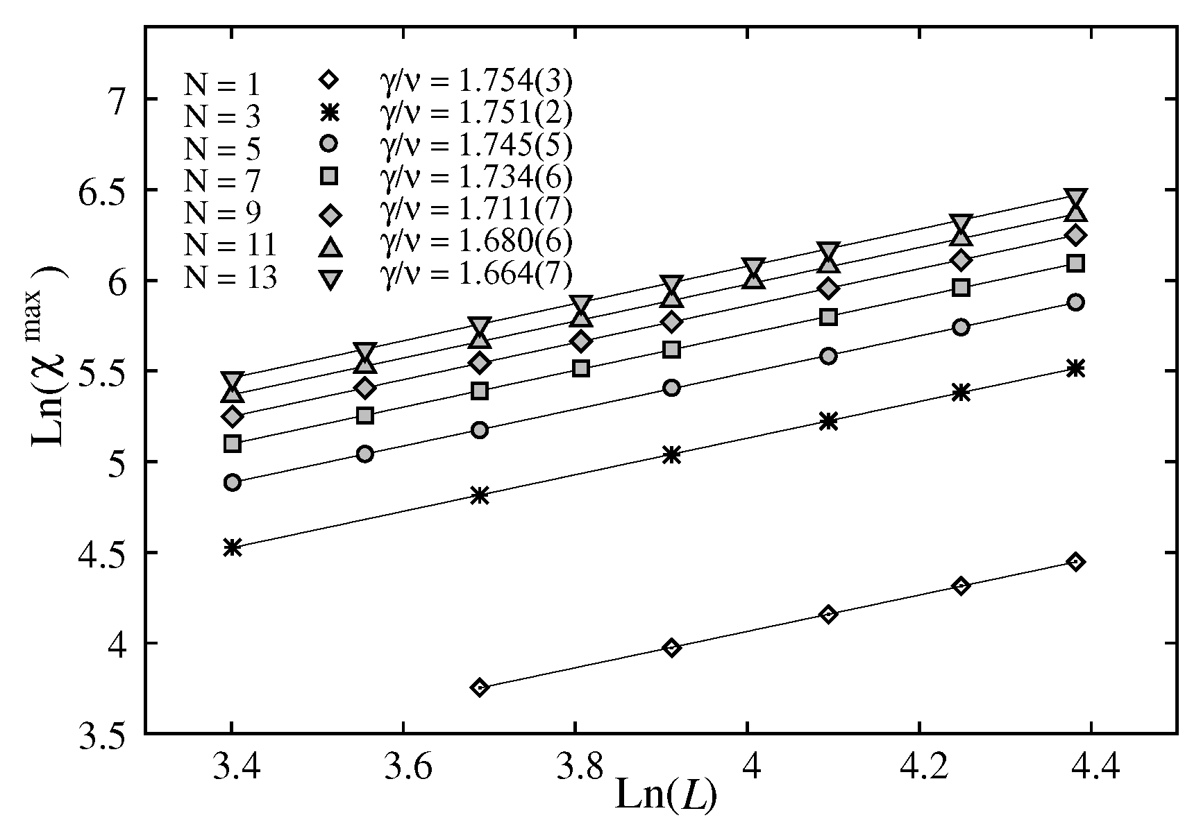
Figure 6.
Maximum of susceptibility versus L in the scale. The slopes give indicated on the figure.
Figure 6.
Maximum of susceptibility versus L in the scale. The slopes give indicated on the figure.
Figure 7.
Exponent versus .
Figure 7.
Exponent versus .
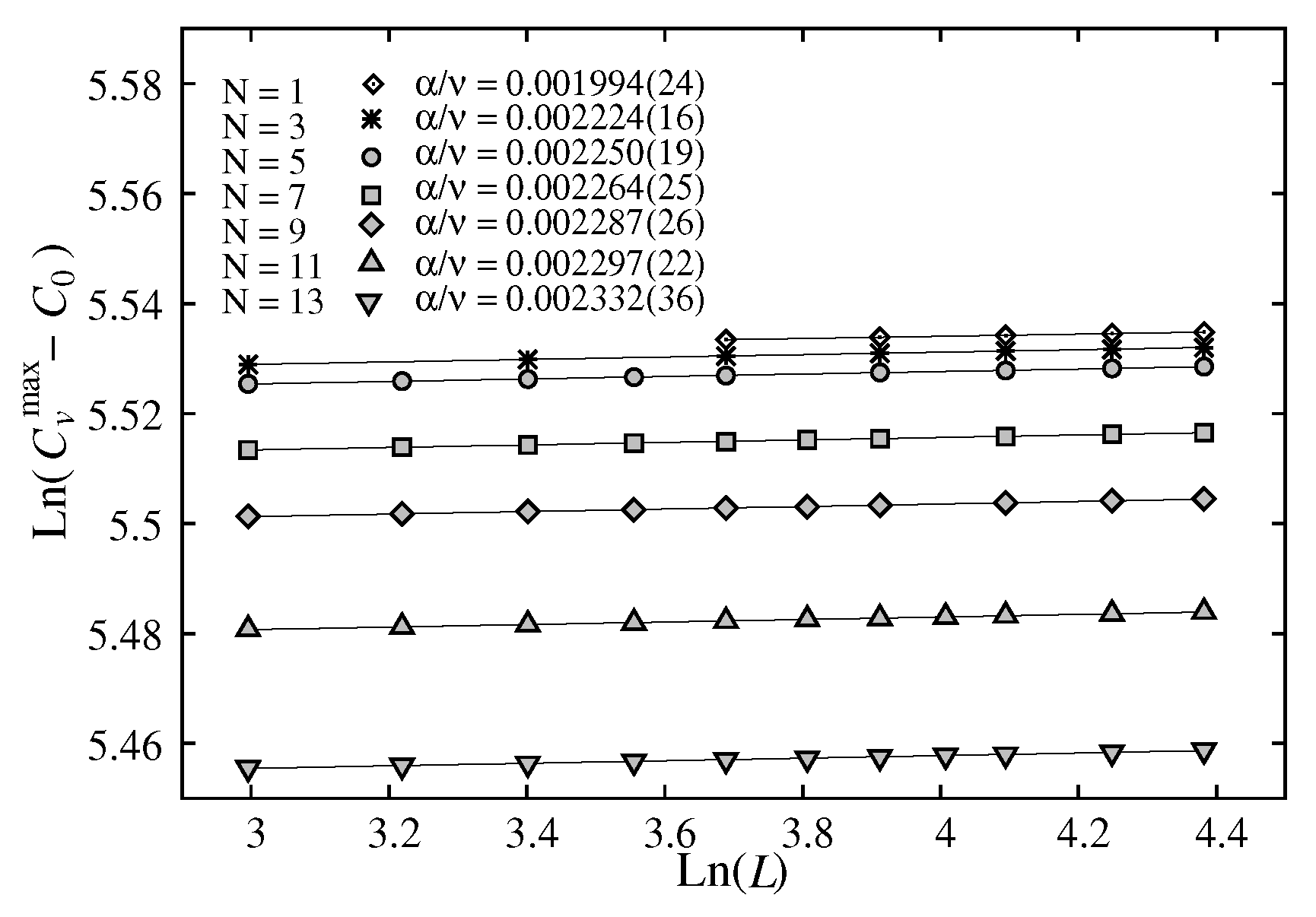
Figure 8.
versus
for
. The slope gives
(see Eq.
9) indicated on the figure.
Figure 8.
versus
for
. The slope gives
(see Eq.
9) indicated on the figure.
Figure 9.
(a) and (b) vs L up to 160 with .
Figure 9.
(a) and (b) vs L up to 160 with .
Figure 10.
vs L (a) from 20 up to 160 (b) from 70 up to 160, for .
Figure 10.
vs L (a) from 20 up to 160 (b) from 70 up to 160, for .
Figure 11.
Exponent as a function of the film thickness.
Figure 11.
Exponent as a function of the film thickness.
Figure 12.
Effective dimension of thin film defined by , as a function of thickness. See text for comments.
Figure 12.
Effective dimension of thin film defined by , as a function of thickness. See text for comments.
Figure 13.
Critical temperature at infinite
L,
, versus
. MC results are shown by points, continuous line is the prediction of Capehart and Fisher, Eq. (
17). The agreement is excellent.
Figure 13.
Critical temperature at infinite
L,
, versus
. MC results are shown by points, continuous line is the prediction of Capehart and Fisher, Eq. (
17). The agreement is excellent.
Figure 14.
Maximum of versus L in the scale for : (a) without PBC in z direction (b) with PBC in z direction. The slopes are indicated on the figure.
Figure 14.
Maximum of versus L in the scale for : (a) without PBC in z direction (b) with PBC in z direction. The slopes are indicated on the figure.
Figure 15.
versus L in the scale for (a) without PBC in z direction (b) with PBC in z direction. The data points of two cases are not distinguishable in the figure scale. The slopes are indicated on the figure.
Figure 15.
versus L in the scale for (a) without PBC in z direction (b) with PBC in z direction. The data points of two cases are not distinguishable in the figure scale. The slopes are indicated on the figure.
Figure 16.
(a) Energy of the bulk case vs T for FCC cells, i. E. the number of spins is ; (b) Energy histogram with periodic boundary conditions in all three directions (continuous line) and without PBC (dotted line) in z direction. The histogram was recorded at the transition temperature for each case (indicated on the figure).
Figure 17.
Energy histogram for with film thickness of 8 atomic layers at , respectively.
Figure 17.
Energy histogram for with film thickness of 8 atomic layers at , respectively.
Figure 18.
The latent heat
as a function of thickness
(points are MC results). The latent heat goes to zero at
, i.e. at
atomic layers. The continuous line is the fitted function Eq . (
18).
Figure 18.
The latent heat
as a function of thickness
(points are MC results). The latent heat goes to zero at
, i.e. at
atomic layers. The continuous line is the fitted function Eq . (
18).
Figure 19.
Energy versus temperature T for for a 4-layer film.
Figure 19.
Energy versus temperature T for for a 4-layer film.
Figure 20.
Layer magnetizations for with a 4-layer film: the higher (lower) curve is the surface (beneath) layer magnetization.
Figure 20.
Layer magnetizations for with a 4-layer film: the higher (lower) curve is the surface (beneath) layer magnetization.
Figure 21.
Specific heat are shown for various linear plane sizes L versus T for a 4-layer film.
Figure 21.
Specific heat are shown for various linear plane sizes L versus T for a 4-layer film.
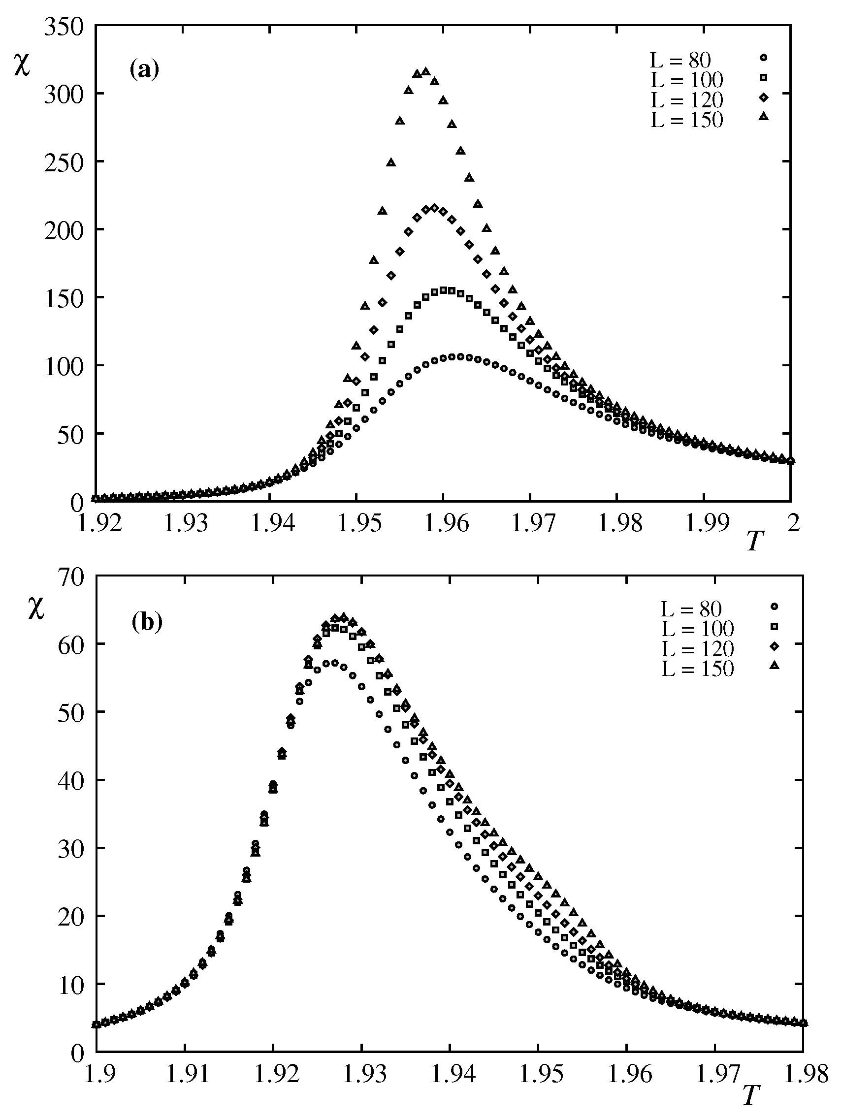
Figure 22.
Susceptibilities of the first layer (a) and the second layer (b) are shown for various sizes L, versus T in a 4-layer film.
Figure 22.
Susceptibilities of the first layer (a) and the second layer (b) are shown for various sizes L, versus T in a 4-layer film.
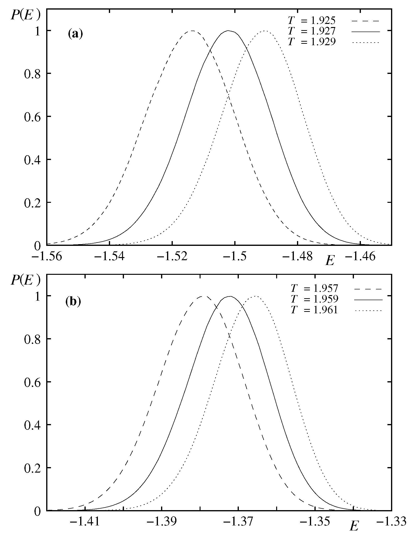
Figure 23.
Energy histograms recorded at temperatures (indicated on the figure) corresponding to the the first (a) and second (b) peaks observed in the specific heat, for with 4-layer film thickness .
Figure 23.
Energy histograms recorded at temperatures (indicated on the figure) corresponding to the the first (a) and second (b) peaks observed in the specific heat, for with 4-layer film thickness .
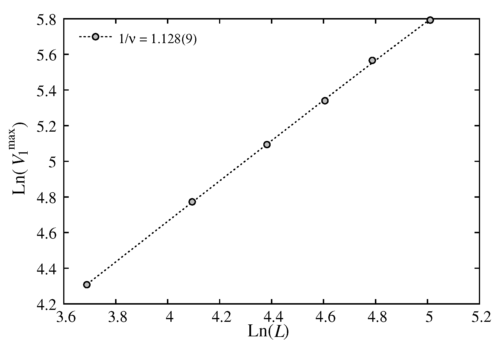
Figure 24.
The maximum value of as a function of L in the scale. The slope of this straight line gives . See the value of in the text.
Figure 24.
The maximum value of as a function of L in the scale. The slope of this straight line gives . See the value of in the text.
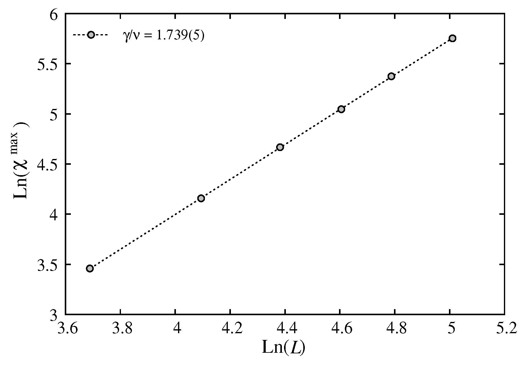
Figure 25.
The maximum of the susceptibility as a function of L in the scale. The slope of this straight line gives . See the value of in the text.
Figure 25.
The maximum of the susceptibility as a function of L in the scale. The slope of this straight line gives . See the value of in the text.
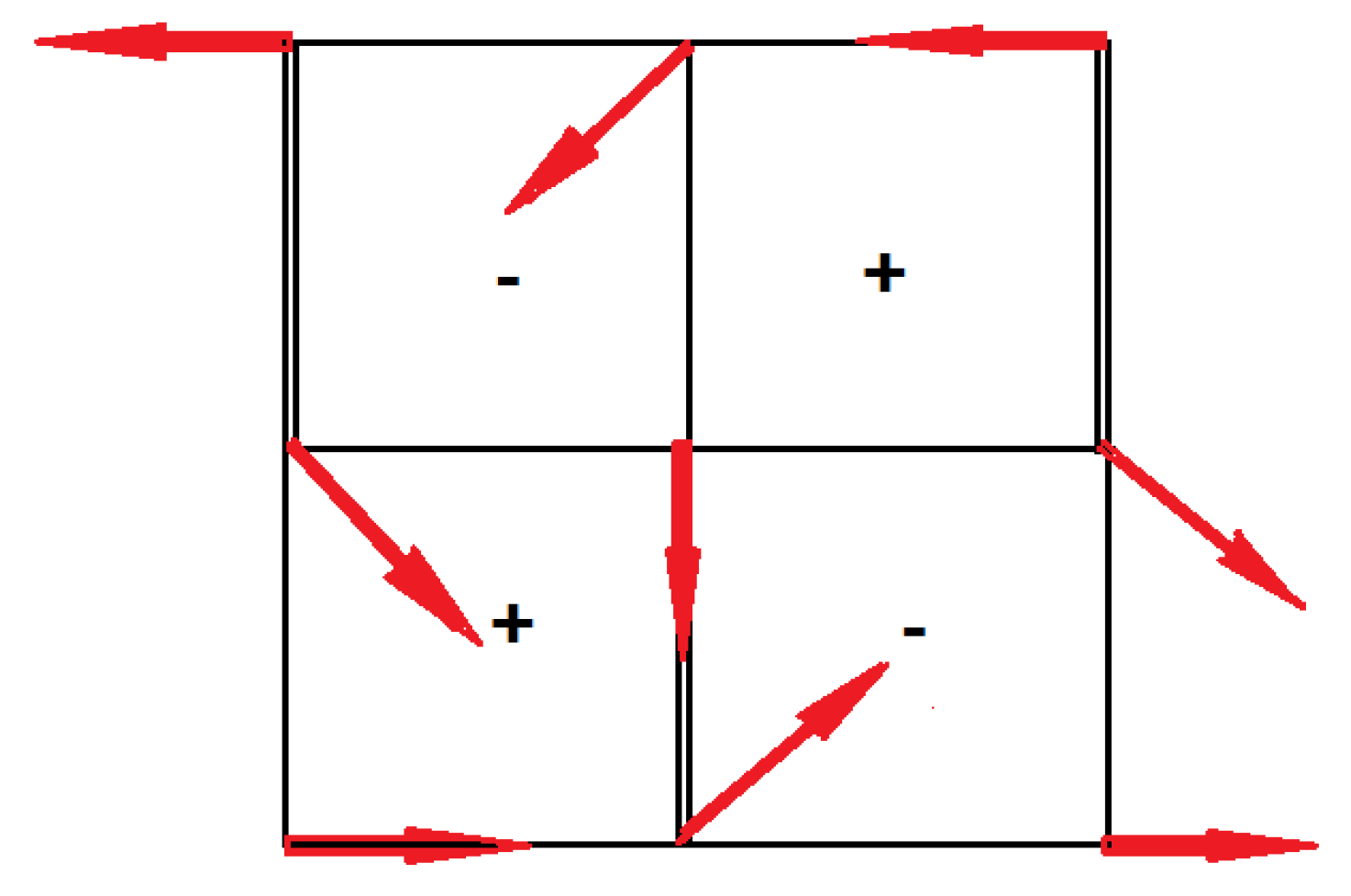
Figure 26.
The square lattice: single (double) bonds are ferromagnetic (antiferromagnetic) bonds. The GS spin configuration is shown by red arrows. The right and left chiralities are denoted by "+" and "-".
Figure 26.
The square lattice: single (double) bonds are ferromagnetic (antiferromagnetic) bonds. The GS spin configuration is shown by red arrows. The right and left chiralities are denoted by "+" and "-".
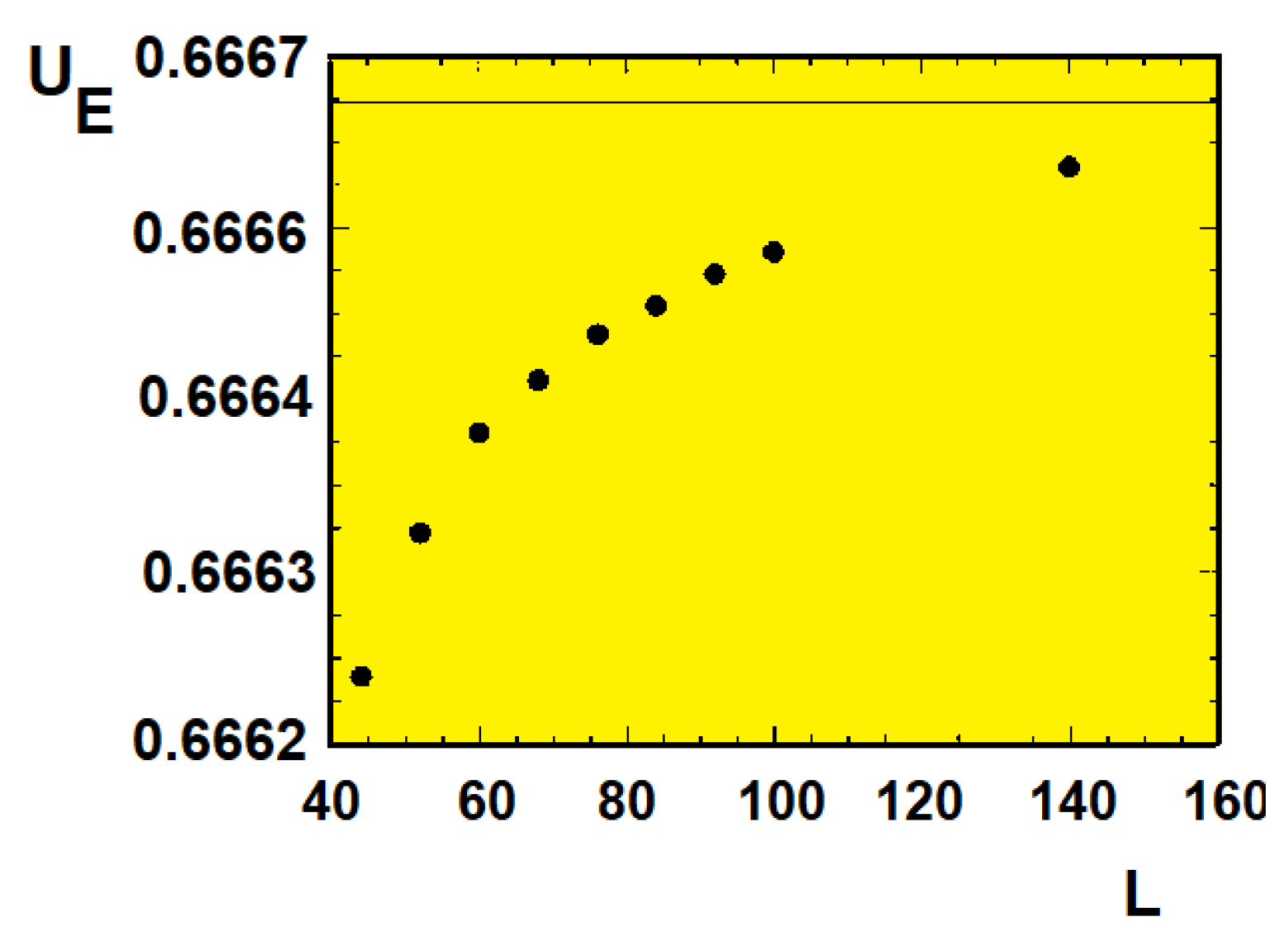
Figure 27.
The Binder energy cumulant versus L calculated at . The horizontal line indicates . The results show that the transition is of second order.
Figure 27.
The Binder energy cumulant versus L calculated at . The horizontal line indicates . The results show that the transition is of second order.
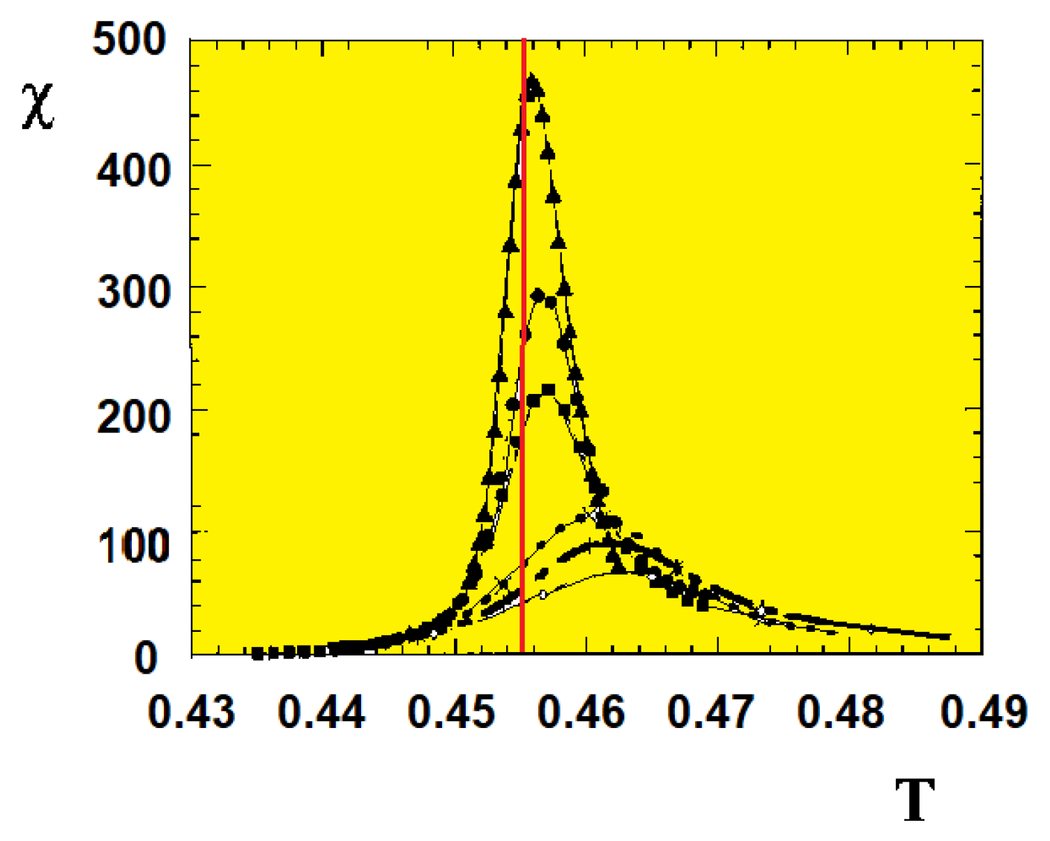
Figure 28.
Susceptibility
versus
T for sizes
(from lowest to highest curves). The red vertical line is the position of
calculated with Eq. (TCL) using
obtained by
Figure 29 below.
Figure 28.
Susceptibility
versus
T for sizes
(from lowest to highest curves). The red vertical line is the position of
calculated with Eq. (TCL) using
obtained by
Figure 29 below.
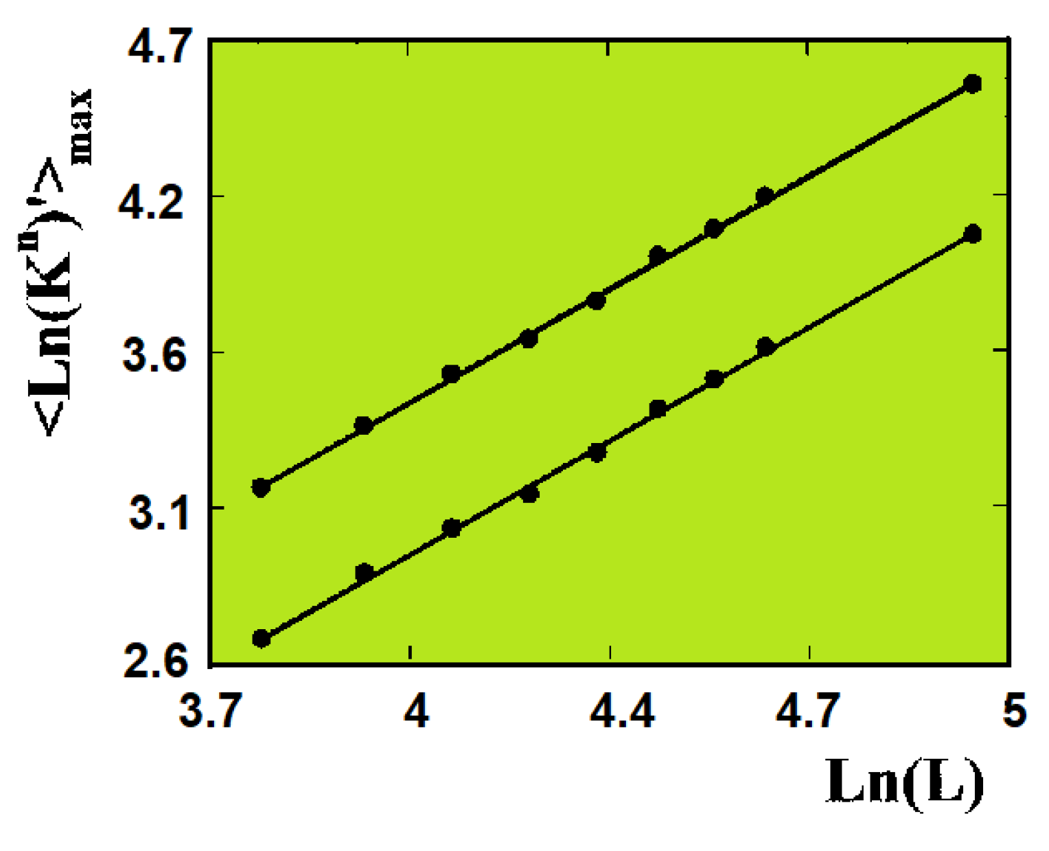
Figure 29.
The maximum of cumulants and versus size in the scale. The slopes give the same . See text for the value of .
Figure 29.
The maximum of cumulants and versus size in the scale. The slopes give the same . See text for the value of .
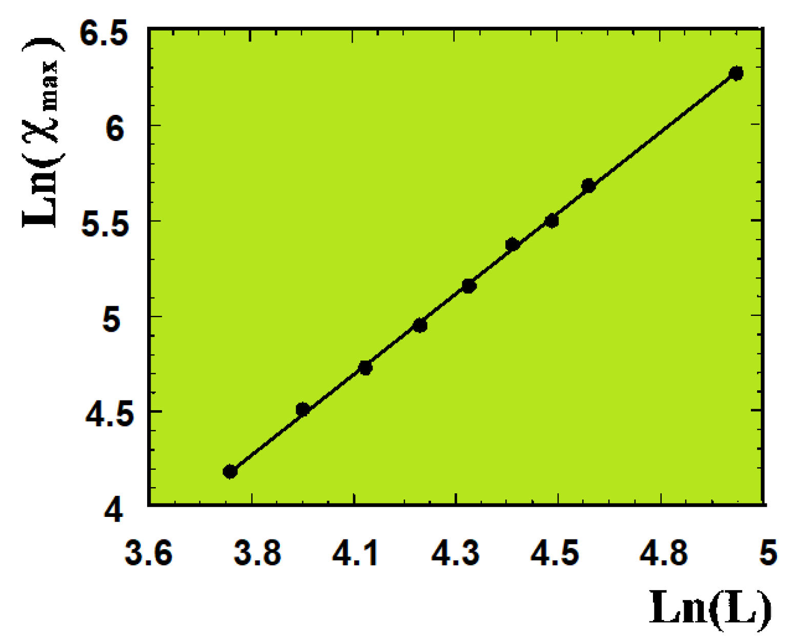
Figure 30.
The maximum of susceptibility versus size in the scale. The slope indicates the value of . See text for the value of .
Figure 30.
The maximum of susceptibility versus size in the scale. The slope indicates the value of . See text for the value of .
Table 1.
Critical exponents obtained by multti-histogram technique. The effective dimension and critical temperature are listed in the last two columns. See text for the definition of the effective dimension .
Table 1.
Critical exponents obtained by multti-histogram technique. The effective dimension and critical temperature are listed in the last two columns. See text for the definition of the effective dimension .
|
|
|
|
|
|
|
| 1 |
|
|
|
|
|
|
| 3 |
|
|
|
|
|
|
| 5 |
|
|
|
|
|
|
| 7 |
|
|
|
|
|
|
| 9 |
|
|
|
|
|
|
| 11 |
|
|
|
|
|
|
| 13 |
|
|
|
|
|
|
Table 2.
Critical exponents obtained by multti-histogram technique for different
Q.
a: Results from Ref. [
40],
b: Results from Ref. [
41]
Table 2.
Critical exponents obtained by multti-histogram technique for different
Q.
a: Results from Ref. [
40],
b: Results from Ref. [
41]
| Q |
|
|
|
|
|
| 8 |
|
|
|
|
|
| 5 |
|
|
|
|
|
| 4 |
|
|
|
|
|
| 3D Ising |
|
|
|
|
|
| 3 |
|
|
|
|
|
| 3D XY |
|
|
|
|
|