Submitted:
21 February 2025
Posted:
24 February 2025
You are already at the latest version
Abstract
Studying the spatial distribution patterns, intraspecific and interspecific associations of tree species are crucial for understanding the maintenance of biodiversity and offering insights into community dynamics and stability. The Shennongjia National Park, located in the transition zone between the (sub-) tropics and the temperate climate holds great significance for understanding how species interact with each other and coexist within forest communities.
We used data from a full mapped 25-ha montane deciduous broadleaved forest dynamic plot at Shennongjia (SNJ) National Park, central China to conduct a community level evaluation of spatial distribution patterns and intraspecific and interspecific associations. We analyzed spatial distribution pattern of 20 dominant species with univariate and bivariate g(r) functions, as well as the intraspecific and interspecific associations across different life history stages. We assess the relative contributions of underlying processes in community assembly with three models: Complete Spatial Randomness (CSR), Heterogeneous Poisson (HP), and Antecedent Condition (AS). The results showed that all 20 tree species exhibit small-scale aggregation distribution. While, aggregation distribution degree decreased and mainly showed random or uniform distributions when excluded environmental heterogeneity. Positive associations were common in different life history stages. Negative associations were common across different species, while, most of the significant intraspecific and interspecific associations turned to be irrelevant when excluded environmental heterogeneity. We concluded that habitat heterogeneity and dispersal limitation may primarily determine the spatial distribution of species in the subtropical montane deciduous broad-leaved forest. This suggests that the forest is highly sensitive to environmental changes. Upcoming management approaches ought to concentrate on ongoing observation, crucial for mitigating how climate change might affect species distribution and community interactions, thus guaranteeing enduring stability and conservation of biodiversity.
Keywords:
spatial distribution pattern
; environmental heterogeneity
; point pattern analysis
; spatial segregation
; dispersal limitation
; broad-leaved forest
; forest dynamic plot
1. Introduction
Understanding local species interactions within communities is crucial for maintaining species diversity, one of the most important ways to mitigate biodiversity loss, a major driver of global ecosystem change (Wiegand et al. 2021; Ting et al. 2023). Spatial distribution pattern refers to the arrangement of individuals within a geographic area, whether clustered, evenly spaced, or randomly dispersed. These findings uncover fundamental ecological aspects like the intensity of clustering, effects dependent on scale, and populations’ spatial layout, and elucidate how environmental factors, along with local competition both within and between species, impact plant dispersion in specific regions (Janik et al. 2016). Such models play a crucial role in discovering the processes that foster species survival and community structure, especially in intricate ecosystems like mountain deciduous broad-leaved woodlands. They embody plants’ ecological responses to environmental changes and competitive pressures, serving as a vital tool for detecting community assembly rules (Omelko et al., 2018; Zhang et al. 2020), which contribute to the development of effective strategies for biodiversity conservation and forest management (Wiegand et al., 2021; Santos et al. 2020; Ting et al., 2023).
Habitat heterogeneity and dispersal limitation are two key hypotheses explaining the aggregated distribution of tree species. Habitat heterogeneity, rooted in niche-based theory, posits that deterministic factor such as environmental conditions, local species interactions, and resource availability drive species aggregation patterns (Diamond, 1975; Weiher & Keddy, 1995). Previous studies have shown that the effects of habitat heterogeneity on species distribution accumulate across different life stages, leading to variations in spatial patterns depending on growth stage and habitat type (Clark et al., 1999; Zhang et al., 2012; Baldeck et al., 2013; Shen et al., 2013). The Janzen-Connell theory reinforces this idea, proposing that increased death rates in seeds or seedlings close to original trees, due to predation or particular pests, open avenues for new species to colonize, influencing their distribution and promotin levels (Janzen, 1970; Connell, 1984). Differing from niche-based theory, dispersal restriction is seen as unbiased, suggesting that the patterns of species distribution and community behavior mainly stem from random occurrences like birth, death, movement, and migration restrictions (Hubbell, 2001). This perspective emphasizes the role of random processes in shaping ecological communities, rather than deterministic biotic or abiotic factors. Hubbell et al. (1979) noted, for instance, an almost exponential reduction in seedling density as the distance from the mother tree increases, underscoring the critical role of seed spread processes in shaping the patterns of species clustering. While habitat heterogeneity and dispersal limitation provide significant frameworks for understanding the aggregated distribution of tree species, research on the effects of varying scales of habitat heterogeneity on species distribution and the potential influence of local climate variations on dispersal mechanisms remains insufficient. Further exploration of how species interactions change with fluctuations in environmental conditions can deepen our understanding of community assembly processes and inform effective biodiversity conservation strategies.
Analyzing spatial point patterns is a crucial ecological method for clarifying the spatial spread and connections in plant communities, offering vital understanding of fundamental ecological dynamics (Wiegand and Moloney, 2004). This method categorizes spatial distributions into three primary patterns: clustered (aggregate or clumped), regular (uniform or segregated), and random. Likewise, the spatial correlations among various point types can be classified into categories like attraction (positive correlation), absence of interaction (no correlation), or repulsion (negative correlation) (Wiegand & Moloney, 2013; Ben-Said, 2021). An essential advancement in this method involves replacing Ripley’s K function’s conventional circles with univariate pairwise and pair correlation functions for circles with radius r, opting for circles with a defined width instead. This alteration successfully diminishes the impact of minor aggregate influences, leading to improved precision and dependability in analyzing spatial patterns (Ripley, 1976; Gu et al., 2019). By maximizing the utilization of spatial coordinates of individual plants, this method provides a detailed and nuanced understanding of ecological dynamics, making it an invaluable tool for ecological research and conservation efforts. This study utilizes a range of point methods like the Homogeneous Poisson process, followed by Heterogeneous Poisson process, Homogeneous Thomas process, and again Heterogeneous Thomas process, to analyze point patterns and spatial associations at diverse scales. Such procedures facilitate a numerical evaluation of pattern traits and provide robust explanations for the mechanisms underlying processes of species coexistence (Erfanifard & Stereńczak, 2017; Carrer et al., 2018; Omelko et al., 2018).
Shennongjia National Park lies in a region that acts as an intermediary zone for subtropical and temperate climates, celebrated worldwide for its crucial role in biodiversity preservation. The dominant vegetation in this region is the deciduous broad-leaved forest, primarily composed of Fagaceae species, which are characteristic of Northern Hemisphere forests. Given its high biodiversity and sensitivity to climate change, this transitional forest is of critical importance for studying species coexistence and developing strategies to better cope with future climate change (Ge et al., 2022). While holding ecological importance, the region necessitates a critical need for extensive ecological studies, especially focusing on tree populations and their community dynamics in large plots. To address this gap, our study aims to investigate the spatial distribution patterns of 20 dominant tree species and their associations within the forest. Specifically, we address the following research questions: (a) Do the mechanisms influencing species spatial distribution vary across different spatial scales? (b) How do intraspecific and interspecific associations vary across different life-history stages? (c) Are the distribution patterns of dominant species consistent across the canopy, sub-canopy, and shrub layers? (d) What ecological processes drive the formation of the observed distribution patterns of dominant species in this forest plot? By addressing these questions, this study explores the role of negative density dependence in shaping the spatial distribution of dominant species in subtropical mountainous forests.
2. Materials and Methods
2.1. Study Site
The study site is located in Shennnongjia National Park (31°24’27.2657” N, 110°23’57.6958” E) in central China. This area is characterized by a mid-subtropical mountain deciduous broad-leaved (Quercus aliena var. acutiserrata - Fagus engleriana) (Figure 1). According to the meteorological station (1700 m a.s.l.), the mean annual temperature was 10.6 °C, Precipitation averaged 1330 mm, mainly in June-October. The relative humidity averages 75%. Due to precipitation, the humidity at the sample site remains high throughout the year, with the highest levels typically occurring in July and the lowest levels typically occurring in April (>70%).
2.2. Data Collection
A 25 ha (500 m × 500 m) forest dynamic plot (Shennongjia, SNJ) was established in August 2022, following the protocol of ForestGEO (The Forest Global Earth Observatory). The 25-ha plot was systemically divided into 625 subplots of 20 × 20 m. Within each quadrat, all trees with a diameter at breast height (DBH) ≥ 1 cm were tagged, recorded, measured, identified by species, and mapped. The elevation range of the plot is 1824-2158 m, with an average elevation of 1986.88 m. The plot has a slope of 4.54 - 46.90° over an area of 20 m × 20 m. The direction of the slope ranges from 4.57 - 229.56°, and the degree of convexity ranges from -5.7-8.31. The first censuses showed that there were 149 species (including varieties) and 61,054 individuals (including 97,664 individuals with branches) in this plot, belonging to 44 families and 79 genera, of which 28 were evergreen and 121 were deciduous. The dominant canopy species are Q. aliena var. acuteserrata, F. engleriana, Betula albo-sinensis. The dominant subcanoopy species are Acer pentaphyllum, Lindera trifoliata, Acer tetrastigma. and the shrubs are dominated by Viburnum sibiricum, Phyllanthus thunbergii, Viburnum sibiricum.
We first calculated importance value for each tree species and selected the important value ranked in the top 20 for the latter analyses. The importance value is defined as [(relative abundance + relative basal area + relative frequency)/3] (Table 1). The forest was divided into three vertical layers: canopy layer (≥ 15 m), understory layer (≥ 5 m and < 15 m), and shrub layer (< 5 m) (Zhu et al. 2008). For each selected species, we classified different life-type stages based on DBH values and life form. Canopy layer: 1 cm ≤ DBH < 5 cm (saplings), 5 cm ≤ DBH < 20 cm (juveniles), DBH ≥ 20 cm (adults); understory layer: 1 cm ≤ DBH < 5 cm (saplings), 5 cm ≤ DBH < 10 cm (juveniles), DBH ≥ 10 cm (adults); shrub layer: 1 cm ≤ DBH < 2 cm (saplings), 2 cm ≤ DBH < 3 cm (juveniles), DBH ≥ 3 cm (adults). Then, using the diameter class method, we analyzed the spatial distribution pattern of dominant species within the community. The spatial analysis was less reliable in cases where the number of individuals was low. To meet a large sample size required for accurate point pattern analysis, life stages with fewer than 200 individuals were excluded. Finally, 6 dominant species with maximal importance value were taken into consideration in intraspecific and interspecific association analyses. The number of individuals at different life history stages of the analyzed species were shown in Table 2.
2.3. Data Analysis
2.3.1. Spatial Distribution Pattern
Point pattern analysis offers a thorough understanding of the spatial distribution of communities by analyzing spatial patterns at various sizes (Cressie, 2015). Here, we applied a K function to analyze the distribution patterns for the 20 dominant species at different scales. The K function is derived from the g(r) function, but is more sensitive than the K function in determining how much the points at a given scale depart from the predicted values (Ripley, 1976). The univariate pairwise correlation g(r) function is calculated as:
where r is the spatial scale (m), the K(r) function is the ratio of the expected number of points to the density of sample points in a circle with any point in the study area as its center, and r is the radius (Stoyan 1994, Velázquez et al. 2016). If g(r) > 1, it indicates a clustered distribution. If g(r) < 1, it indicates a regular distribution. If g(r) = 1, it indicates a completely random distribution (Gu et al., 2019). We chose the complete spatial randomness (CSR) and heterogeneous Poisson (HP) models as the null models (Jalilian et al., 2013). The CSR model is often used as the null hypothesis to examine the effect of habitat heterogeneity on spatial distribution, which assumes that the spatial points of the species are independent of each other and not affected by any abiotic or biotic processes. It also assumes that the species have the same probability of occurring at each point in the study area (Gabriel, 2017). And the Heterogeneity Poisson model is a null hypothesis model that excludes the effect of spatial heterogeneity, which can accurately represent the population’s real spatial distribution characteristics.
2.3.2. Intraspecific and Interspecific Associations
Bivariate pairwise correlation functions (PCF) were applied to determine interspecific relationships among the dominant species and intraspecific associations of the six selected dominant species at different life-history stages. The PCF was calculated as:
(i≠j)
Here, i and j represent two distinct populations, while n1 and n2 denote the total number of surviving individuals in populations i and j respectively. When g12(r) >1, it indicates a positive association between the two populations; g12(r) =1 suggests no significant association; and g12(r) <1 reflects a negative association.
The antecedent condition (AC) and the CSR were selected as the null models; the AC null model assumes that the positions of those with smaller DBHs are randomized, while those with bigger DBHs remain unchanged (Wiegand & Moloney, 2004). Due to life-history stages of tree species are sequentially but not realized simultaneously, we first used the AC null model to fix the positions of individuals with larger DBHs, and then analyzed the association between individuals with smaller and larger DBHs.
To assess the accuracy of the empirical function, we performed a 95% simulation envelope with maximum and lowest values and ran 199 Monte Carlo simulations of the null model for all spatial pattern analyses (Baddeley et al., 2014). These analyses were performed by using the “spatstat” package in R 4.2.2 (Baddeley et al., 2015).
3. Results
3.1. Spatial Distribution Pattern
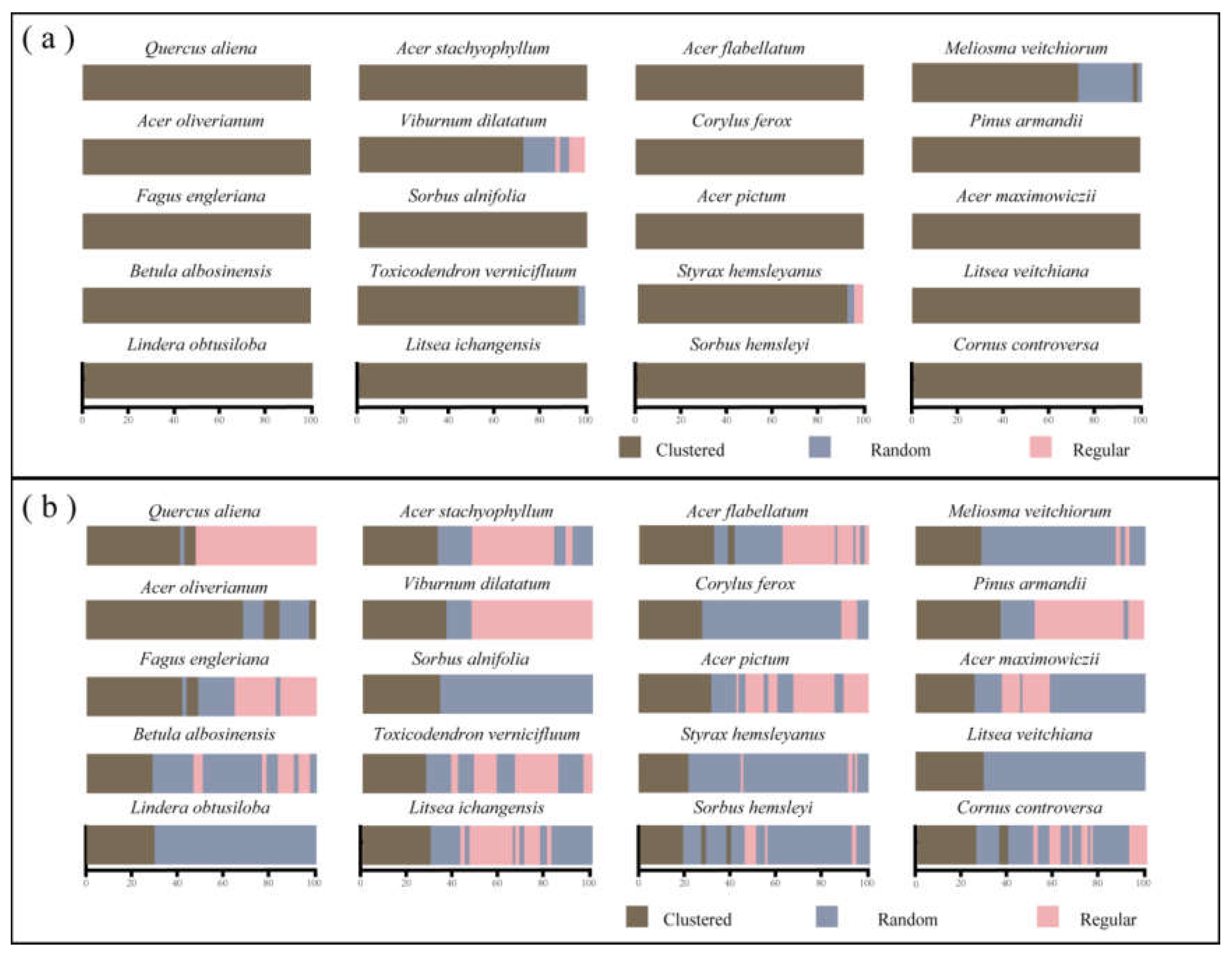
Based on the CSR null model, the results of the univariate g(r) function shown that the 20 dominant tree species had an aggregated spatial pattern across the test area. As the scale increased, the degree of aggregation for most species (16 in 20) decreased significantly. However, there were four species, Viburnum dilatatum, Toxicodendron vernicifluum, Styrax hemsleyanus, and Meliosma veitchiorum, showed distribution patterns other than aggregated distributions (Figure 3a). The actual discrete distribution of each tree species in the SNJ plot was generally consistent with the results of spatial distribution pattern of tree species under CSR (Figure 2). Therefore, the spatial distribution pattern of dominant tree species is mostly aggregate distribution when other contributing factors were not taken into account. In order to further obtain a rough estimate of the large-scale impact of habitat heterogeneity on local tree, we examined the distribution of all 20 species and compared it with the HP null model.
obs(r): Observed value of (r); (r): theoretical mean of g(r); Gay shaded part is the 99 confidence interval.
The HP null model showed that, once the influence of environmental heterogeneity was removed, the distribution pattern of different tree species had undergone significant change (Figure 3b). Compared to the CSR model, the degree of dominating species aggregation was lower in the HP null models. 80% (Sixteen) of tree species showed new patterns of spatial distribution after controlling for environmental heterogeneity (Figure 3b). Specifically, most dominating species (except for Acer oliverianum) showed similar individual distribution patterns, where trees were aggregated at small scales and then distributed equally or randomly as the scale increased. At scales greater than 35 m, the distribution pattern changed to a random distribution after removing environmental heterogeneity, although Lindera obtusiloba, Sorbus alnifolia and Litsea veitchiana all showed aggregated distribution across the scale. With the exception of them, all sixteen species showed three distribution patterns in the HP null model, which differed significantly from the CSR model. Additionally, life stage had an impact on the trees’ distribution patterns. Therefore, we investigated the spatial distribution patterns of dominant species across different life stages.
Figure 3.
The univariate pair correlation function results are presented under CSR and HP null models. Panel (a) indicates the g(r) function under CSR, while panel (b) indicates the g(r) function under HP. The scale r (m) is denoted on the x-axis.
Figure 3.
The univariate pair correlation function results are presented under CSR and HP null models. Panel (a) indicates the g(r) function under CSR, while panel (b) indicates the g(r) function under HP. The scale r (m) is denoted on the x-axis.
3.2. Intraspecific and Interspecific Associations
3.2.1. Intraspecific Patterns from Saplings to Adults
We used bivariate pairwise correlation function (g12 (r) function) to analyze the spatial correlation of 6 dominant species in different life-history stages (Figure 4) based on the null models of CSR and AC.
Under CSR, Acer flabellatum showed positive associations across different life history stages (Figure 4a). There were also significant positive association at all scales between the small and medium trees of Quercus aliena, Acer oliverianum and Fagus engleriana, and between the medium and large trees of Q. aliena and L. obtusiloba. Furthermore, a significant positive correlation was observed among the three life stages of V. dilatatum on a smaller scale (<50 m). However, this correlation was disappeared on a larger scale. After removing the effect of environmental heterogeneity, the results of the AC null model showed no significant associations between small and medium or small and large trees in the tree layer of Q. aliena and A. oliverianum at any scale (Figure 4b). In detail, the life history stages of medium and large trees of Q. aliena and A. flabellatum showed positive associations at the small scale, which shifted to non-significant associations as the scale increased. A shrub species, V. dilatatum only showed positive associations across three stages on the scales less than 15 m, and it turned to be non- significant or negative with scale increases. On a larger scale, small trees and large trees of V. dilatatum were mainly negatively correlated.
Figure 4.
Pair correlation function results of different life stages of six dominant tree species are presented under CSR and AC null models. Panel (a) indicates the g12(r) function under CSR, while panel (b) indicates the g12(r) function under HP. The scale r (m) is denoted on the x-axis.
Figure 4.
Pair correlation function results of different life stages of six dominant tree species are presented under CSR and AC null models. Panel (a) indicates the g12(r) function under CSR, while panel (b) indicates the g12(r) function under HP. The scale r (m) is denoted on the x-axis.

3.2.2. Interspecific Association
We employed the bivariate pair correlation function (g12(r) function) again to analyze the spatial correlation among the six dominant tree species (Figure 5). As shown in Figure 5, Q. aliena and F. engleriana, Q. aliena and V. dilatatum, F. engleriana and L. obtusiloba showed attraction patterns at all scales under the CSR null model, while Q. aliena and A. oliverianum, L. obtusiloba and A. flabellatum showed repulsion patterns at all scales. Meanwhile, Q. aliena and L. obtusiloba, A. oliverianum and V. dilatatum, L. obtusiloba and V. dilatatum, V. dilatatum and A. flabellatum were positively correlated at small scales, followed by no or negative correlations as the scales increased. Trees of Q. aliena were significantly positively associated with small trees of A. flabellatum at scales of less than 80 m, though they were no significant correlation between them on some scales. The spatial correlation between tree species A. flabellatum and F. engleriana was similar to that of these two species. On the scales of less than 5 m, there was no significant correlation between A. oliverianum and A. flabellatum, while on the scales of more than 5 m, there was a significant negative correlation.
However, the analysis results under the AC showed that the correlation among tree species had changed significantly on a large scale, mainly showing a lack of significant associations after excluding the influence of environmental heterogeneity (Figure 5). Compared to the CSR null model, the associations between different species were different on most scales, which was reflected in the irrelevance between species on most scales. Specifically, at the scale of more than 50%, the spatial correlation was non-associated the except for A. oliverianum and V. dilatatum. In contrast to the predominant lack of correlation, A. oliverianum and V. dilatatum showed a positive correlation at the 0-33, 35-36, 38-39, and 43-45 m scales, F. engleriana and A. flabellatum showed a negative correlation at the 0-46 and 49-53 m scales. These results indicate that environmental heterogeneity has a substantial impact on the relationships among dominant species.
Figure 5.
Pair correlation function results of different dominant tree species are presented under CSR and AC null models. Panel (a) indicates the g12(r) function under CSR, while panel (b) indicates the g12(r) function under HP. The scale r (m) is denoted on the x-axis.
Figure 5.
Pair correlation function results of different dominant tree species are presented under CSR and AC null models. Panel (a) indicates the g12(r) function under CSR, while panel (b) indicates the g12(r) function under HP. The scale r (m) is denoted on the x-axis.

4. Discussion
4.1. Spatial Distributions of Dominant Species
In this study, we explored the spatial patterns of tree species under two models—CSR (Completely Spatially Random) and HP (Habitat Patchiness)—to test the applicability of the Janzen-Connell hypothesis, which posits that seedling survival decreases with proximity to parent trees due to density-dependent mortality and herbivory (Janzen, 1970; Connell, 1971). The CSR model revealed that all species showed clustered patterns over a broad spatial range, possibly because of restricted seed dispersal and habitat preferences (Liu et al., 2012; He et al., 2021). However, considering habitat heterogeneityin the HP model led to a narrowed aggregate distribution spectrum and a transition of spatial layouts to a more uniform or random pattern, becoming predominant there. This shift highlights the significant role of habitat patches in shaping species distribution patterns (Shen et al., 2013; Perea et al., 2021). This research aligns with earlier works indicating species typically group at smaller scales and show either random or consistent distribution over larger scales (Liu et al., 2012; Shen et al., 2013). The Janzen-Connell theory offers a credible explanation for the noted trends. Within the smaller scope (0-20 meters), the 20 primary species in our research demonstrated clustered dispersal, mainly attributed to the constraints of movement (Seidler & Plotkin, 2006; Zhou et al., 2019). For instance, Q. aliena var. acuteserrata (a nut species) has large, heavy seeds that are dispersed mainly by gravity, resulting in high seedling density around parent trees. In contrast, A. pentaphyllum (a samara species) can disperse its seeds over longer distances due to its winged morphology, allowing seedlings to establish in suitable environments away from the parent tree. With the expansion in scale, aggregation levels diminish, in line with the Janzen-Connell theory suggesting an exponential reduction in seedling density as the distance from the originating tree grows (Hubbell, 1979).
In addition to dispersal limitations, habitat heterogeneity also plays a crucial role in shaping species distribution patterns at larger scales (Lin et al., 2011; Shen et al., 2009). Results from the HP model revealed that small parts of habitats have a notable effect on the distribution of species. For example, Q. aliena var. acuteserrata prefers well-drained, moist, neutral to slightly acidic soils, while F. engleriana thrives in fertile, acidic soils with cool and humid climates. A. oliverianum is adapted to sunny, drought-tolerant environments, often found at forest edges or in sunny gaps. Pinus armandii can tolerate a variety of soils but is sensitive to high temperatures. Betula albosinensis, S. alnifolia, and T. vernicifluum mainly aggregated on sunny slopes, which was similar to the research of Liu et al. (2014) and Wang et al. (2024), showing that clustering density increases with the terrain (slope position, slope direction and slope gradient). These habitat preferences lead to aggregated distributions in locally suitable environments, further supporting the role of habitat heterogeneity in shaping species distribution patterns (Getzin et al., 2008, Beyns et al., 2021).
The aggregated distribution at small scales may also be related to the high niche overlap among the dominant species, especially among small and medium-sized individuals. This aggregation can enhance population-level effects, increase interspecific competition, and ensure long-term population persistence (Hardy & Sonké, 2004; Dohn et al., 2017). For example, the canopy layer species showed higher aggregation at larger scales, likely because species with higher population densities tend to cluster more strongly (Figure 2). In summary, the spatial distribution patterns of tree species in natural plant communities are influenced by both habitat heterogeneity and dispersal limitations. Future research should further explore the mechanisms underlying these patterns and their implications for community dynamics and conservation.
4.2. Associations Across Species and Life-History Stages
In this study, the six dominant species generated 15 groups of species pairing patterns, which were dominated by positive and negative correlations under the CSR model and by non-correlation under the AC model. These findings are inconsistent with those of Yang et al. (2022) in the karst secondary forest in central Guizhou, where the interrelationships among the four dominant species mainly showed negative or no correlation. This discrepancy may be related to differences in life forms, climate types, and topography among the dominant species. These results can be interpreted through the lens of the Species Herd Protection hypothesis (Peters, 2003; Lin et al., 2013), which suggests that species interactions are influenced by both resource competition and mutual benefits.
Positive correlations between species indicate a high similarity in resource use and niche overlap. The stronger the positive correlation, the greater the complementarity between populations within the community, leading to more efficient resource utilization and enhanced community stability. Under the CSR model, eight species pairing patterns in this study showed positive correlations across most scales. This result may be attributed to high niche overlap among these species. For example, Q. aliena var. acuteserrata exhibited positive correlations with several other species, suggesting that they share similar resource requirements but may benefit from mutual facilitation. This finding aligns with the Species Herd Protection hypothesis, which posits that when mutual benefits between species outweigh interspecific competition, species will exhibit attraction (Peters, 2003). This hypothesis is also supported by recent studies on species abundance and interaction intensity in ecological networks, which show that interaction strength is strongly related to species abundance (Vázquez et al., 2007; Wang et al., 2010). The greater the chance of two species encountering each other, the stronger their interaction.
Negative correlations between species indicate niche space isolation and competition. In this study, six species pairs mainly exhibited negative correlations under the CSR model. For example, Q. aliena var. acuteserrata had a negative correlation with A. oliverianum and A. flabellatum. These species are heliophilous plants, suggesting strong competition for light and other resources. Spatial separation may be a strategy to reduce competitive consumption. Notably, A. flabellatum showed strong negative correlations with four dominant species, except for V. dilatatum, which were primarily concentrated in the high-altitude northern area of the plot. Resource competition is likely the main reason for this exclusionary effect. Given the limited space and resources, plants compete for light, water, nutrients, and space, resulting in mutual exclusion. This finding supports the idea that competition drives spatial segregation among species, as predicted by the Species Herd Protection hypothesis. Non-correlations between species indicate a lack of significant interactions, which may result from spatial isolation or environmental heterogeneity. Under the AC model, non-correlation accounted for a larger scale range, suggesting that after accounting for environmental heterogeneity, interspecific associations were independent of each other across broader scales. This finding suggests that spatial separation of species on a larger scale can hinder interactions between two species. Additionally, aggregation within species can lead to large-scale spatial separation between species (Pacala, 1997; Pacala & Levin, 1997). This pattern may explain the observed non-correlations in our study.
5. Conclusions
This study focused on the spatial distribution patterns and intraspecific and interspecific associations of dominant tree species in the deciduous broad-leaved forest of the mid-subtropical mountain in Shennongjia, China. The results show that 20 dominant tree species are clustered on a small scale, and with the increase of scale, the degree of aggregation gradually decreases and changes to random or uniform distribution. The spatial distribution of dominant tree species is mainly affected by environmental heterogeneity and diffusion restrictions. The intraspecific association was mainly a positive correlation, indicating that the population was well connected. Interspecific associations are mainly influenced by the biological characteristics and environmental heterogeneity of each species. These fundings confirm that habitat heterogeneity and dispersal limitation are the two primary drivers of species spatial distributions and potentially shape species coexistences in the subtropical deciduous broad-leaved forest. Spatial distribution pattern is the first step to understanding the plant community structure and revealing the mechanism of species coexistence, and the influence intensity of different factors on species coexistence needs further investigation and research.
Acknowledgments
This study was funded by the National Natural Science Foundation of China (32471622) and Project of Background Resources Survey in Shennongjia National Park (SNJNP2022001), and Open Project Fund of Hubei Provincial Key Laboratory for Conservation Biology of Shennongjia Snub-nosed Monkeys (SNJGKL2022001). We are grateful for the support from Science Research Institute of Shennongjia National Park and helped by Xinzeng Wei, Hao Wu, Shitong Wang, Yuanzhi Qin, Shuaishuai Song, Dong Zhang, Xuefen Xiong and all other contributors involved in completing the construction of the Shennongjia plot.
References
- Baddeley, A., P. J. Diggle, A. Hardegen, T. Lawrence, R. K. Milne, and G. Nair. 2014. On tests of spatial pattern based on simulation envelopes. Ecological Monographs 84:477-489.
- Baddeley, A. J., E. Rubak, and T. R. Turner. 2015. Analysing Spatial Point Patterns with R. Crc Press.
- Baldeck, C. A., K. E. Harms, J. B. Yavitt, R. John, B. L. Turner, R. Valencia, H. Navarrete, S. Bunyavejchewin, S. Kiratiprayoon, A. Yaacob, M. N. N. Supardi, S. J. Davies, S. P. Hubbell, G. B. Chuyong, D. Kenfack, D. W. Thomas, and J. W. Dalling. 2013. Habitat filtering across tree life stages in tropical forest communities. Proceedings of the Royal Society B-Biological Sciences 280.
- Ben-Said, M. 2021. Spatial point-pattern analysis as a powerful tool in identifying pattern-process relationships in plant ecology: an updated review. Ecological Processes 10.
- Beyns, R., D. Bauman, and T. Drouet. 2021. Fine-scale tree spatial patterns are shaped by dispersal limitation which correlates with functional traits in a natural temperate forest. Journal of Vegetation Science 32.
- Carrer, M., D. Castagneri, I. Popa, M. Pividori, and E. Lingua. 2018. Tree spatial patterns and stand attributes in temperate forests: The importance of plot size, sampling design, and null model. Forest Ecology and Management 407:125-134.
- Clark, D. B., M. W. Palmer, and D. A. Clark. 1999. Edaphic factors and the landscape-scale distributions of tropical rain forest trees. Ecology 80:2662-2675.
- Connell, J. H., J. G. Tracey, and L. J. Webb. 1984. Compensatory Recruitment, Growth, and Mortality as Factors Maintaining Rain-Forest Tree Diversity. Ecological Monographs 54:141-164.
- Cressie, N. A. C. 2015. Statistics for Spatial Data, Revised Edition. Statistics for Spatial Data, Revised Edition.
- Dohn, J., D. J. Augustine, N. P. Hanan, J. Ratnam, and M. Sankaran. 2017. Spatial vegetation patterns and neighborhood competition among woody plants in an East African savanna. Ecology 98:478-488.
- Erfanifard, Y., and K. Stereńczak. 2017. Intra- and interspecific interactions of Scots pine and European beech in mixed secondary forests. Acta Oecologica 78:15-25.
- Gabriel, E. 2017. A. Baddeley, E. Rubak, R. Turner: Spatial Point Patterns: Methodology and Applications with R. Mathematical geosciences.
- Gadow, K. V., C. Y. Zhang, C. Wehenkel, A. Pommerening, and X. H. Zhao. 2012. Forest Structure and Diversity. Springer Netherlands.
- Ge, J., Ma, B., Xu, W. et al. 2022. Temporal shifts in the relative importance of climate and leaf litter traits in driving litter decomposition dynamics in a Chinese transitional mixed forest. Plant Soil 477, 679–692.
- Getzin, S., T. Wiegand, K. Wiegand, and F. L. He. 2008. Heterogeneity influences spatial patterns and demographics in forest stands. Journal of Ecology 96:807-820.
- Gu, L., K. L. O’Hara, W. z. Li, and Z. w. Gong. 2019. Spatial patterns and interspecific associations among trees at different stand development stages in the natural secondary forests on the Loess Plateau, China. Ecology and Evolution.
- Hardy, O. J., and B. Sonké. 2004. Spatial pattern analysis of tree species distribution in a tropical rain forest of Cameroon:: assessing the role of limited dispersal and niche differentiation. Forest Ecology and Management 197:191-202.
- Hubbell, S. P. 1979. Tree Dispersion, Abundance, ai Diversity in a Tropical Dry Fore That tropical trees are clumped, not spac, alters conceptions of the organization and dynami. Science.
- Jalilian, A., Y. Guan, and R. Waagepetersen. 2013. Decomposition of Variance for Spatial Cox Processes. Scandinavian Journal of Statistics.
- Janik, Kral, Adam, Hort, Samonil, Unar, Vrska, and McMahon. 2016. Tree spatial patterns of Fagus sylvatica expansion over 37 years. Forest Ecology and Management 2016,375:134-145.
- Janzen, D. 1970. Herbivores and the number of tree species in tropical forests. American Naturalist 104.
- Kenkel, N. C., M. L. Hendrie, and I. E. Bella. 1997. A long-term study of Pinus banksiana population dynamics. Journal of Vegetation Science 8:241-254.
- Lin, G., D. Stralberg, G. Gong, Z. Huang, W. Ye, and L. Wu. 2013. Separating the effects of environment and space on tree species distribution: from population to community. Public Library of Science.
- Nguyen, H. H., J. Uria-Diez, K. Wiegand, and R. Michalet. 2016. Spatial distribution and association patterns in a tropical evergreen broad-leaved forest of north-central Vietnam. Journal of Vegetation Science 27.
- Omelko, A., O. Ukhvatkina, A. Zhmerenetsky, L. Sibirina, T. Petrenko, and M. Bobrovsky. 2018. From young to adult trees: How spatial patterns of plants with different life strategies change during age development in an old-growth Korean pine-broadleaved forest. Forest Ecology and Management 411:46-66.
- Perea, A. J., T. Wiegand, J. L. Garrido, P. J. Rey, and J. M. Alcántara. 2021. Legacy effects of seed dispersal mechanisms shape the spatial interaction network of plant species in Mediterranean forests. Journal of Ecology 109:3670-3684.
- Peters, H. A. 2003. Neighbour-regulated mortality: the influence of positive and negative density dependence on tree populations in species-rich tropical forests. Ecology Letters 6:757-765.
- Ripley, B. D. 1976. 2nd-Order Analysis of Stationary Point Processes. Journal of Applied Probability 13:255-266.
- Seidler, T. G., and J. B. Plotkin. 2006. Seed dispersal and spatial pattern in tropical trees. Plos Biology 4:2132-2137.
- Shen, G. C., F. L. He, R. Waagepetersen, I. F. Sun, Z. Q. Hao, Z. S. Chen, and M. J. Yu. 2013. Quantifying effects of habitat heterogeneity and other clustering processes on spatial distributions of tree species. Ecology 94:2436-2443.
- Stoyan, D. 1994. Caution with Fractal Point Patterns. Statistics 25:267-270.
- Ting, L., R. Zhao, N. J. Wang, L. Xie, Y. Y. Feng, Y. Li, H. Ding, and Y. M. Fang. 2023. Spatial distributions of intra-community tree species under topographically variable conditions. Journal of Mountain Science 20:391-402.
- Vázquez, D. P., C. J. Melián, N. M. Williams, N. Blüthgen, B. R. Krasnov, and R. Poulin. 2007. Species abundance and asymmetric interaction strength in ecological networks. Oikos 116:1120-1127.
- Velázquez, E., I. Martínez, S. Getzin, K. A. Moloney, and T. Wiegand. 2016. An evaluation of the state of spatial point pattern analysis in ecology. Ecography 39:1042-1055.
- Wang, X. G., T. Wiegand, Z. Q. Hao, B. H. Li, J. Ye, and F. Lin. 2010. Species associations in an old-growth temperate forest in north-eastern China. Journal of Ecology 98:674-686.
- Wiegand, T., and K. A. Moloney. 2004. Rings, circles, and null-models for point pattern analysis in ecology. Oikos 104:209-229.
- Wiegand, T., and K. A. Moloney. 2013. A Handbook of Spatial Point Pattern Analysis in Ecology. A Handbook of Spatial Point Pattern Analysis in Ecology.
- Wiegand, T., X. G. Wang, K. J. Anderson-Teixeira, N. A. Bourg, M. Cao, X. Q. Ci, S. J. Davies, Z. Q. Hao, R. W. Howe, W. J. Kress, J. Y. Lian, J. Li, L. X. Lin, Y. C. Lin, K. P. Ma, W. McShea, X. C. Mi, S. H. Su, I. F. Sun, A. Wolf, W. H. Ye, and A. Huth. 2021. Consequences of spatial patterns for coexistence in species-rich plant communities. Nature Ecology & Evolution 5:965-+.
- Zhang, L. Y., L. B. Dong, Q. Liu, and Z. G. Liu. 2020. Spatial Patterns and Interspecific Associations During Natural Regeneration in Three Types of Secondary Forest in the Central Part of the Greater Khingan Mountains, Heilongjiang Province, China. Forests 11.
- Zhang, Y. T., J. M. Li, S. L. Chang, X. Li, and J. J. Lu. 2012. Spatial distribution pattern of population in the Middle Tianshan Mountains and the relationship with topographic attributes. Journal of Arid Land 4:457-468.
- Zhou, Q., H. Shi, X. Shu, F. L. Xie, K. R. Zhang, Q. F. Zhang, and H. S. Dang. 2019. Spatial distribution and interspecific associations in a deciduous broad-leaved forest in north-central China. Journal of Vegetation Science 30:1153-1163.
- Zhu, Y., Zhao, G. F., Zhang, L. W., Shen, G. C., Mi, X. C., Ren, H. B., Yu, M. J., Chen, J. H., Chen, S. W., Fang, T, Ma, K. P. 2008. Community composition and structure of Gutianshan forest dynamics plot in a mid-subtropical evergreen broad-leaved forest, East China. Journal of Plant Ecology (Chinese Version), 32, 262-273. (in Chinese with English abstract).
Figure 1.
Location of the 25 hm2 Shennongjia (SNJ) plot in Shennongjia and in Hubei.
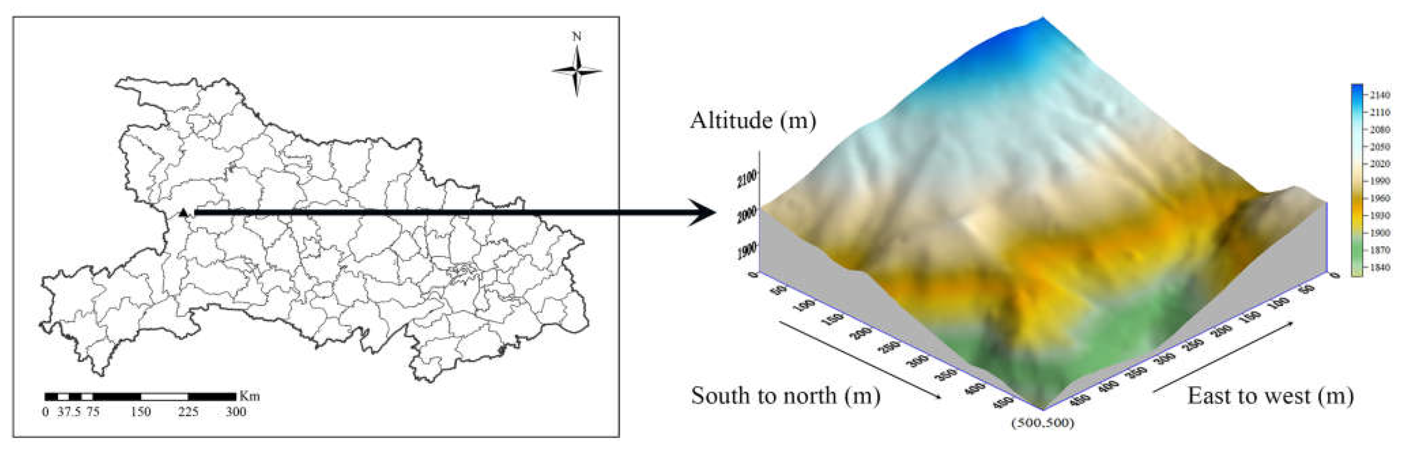
Figure 2.
Univariate intraspecific analysis of the 20 dominant adult species under the CSR model in the 25 SNJ plot. The inserts show the distribution maps of all individuals of the tree species. The black solid line indicates the observed value of g(r), the red dashed line indicates the theoretical value of g(r).
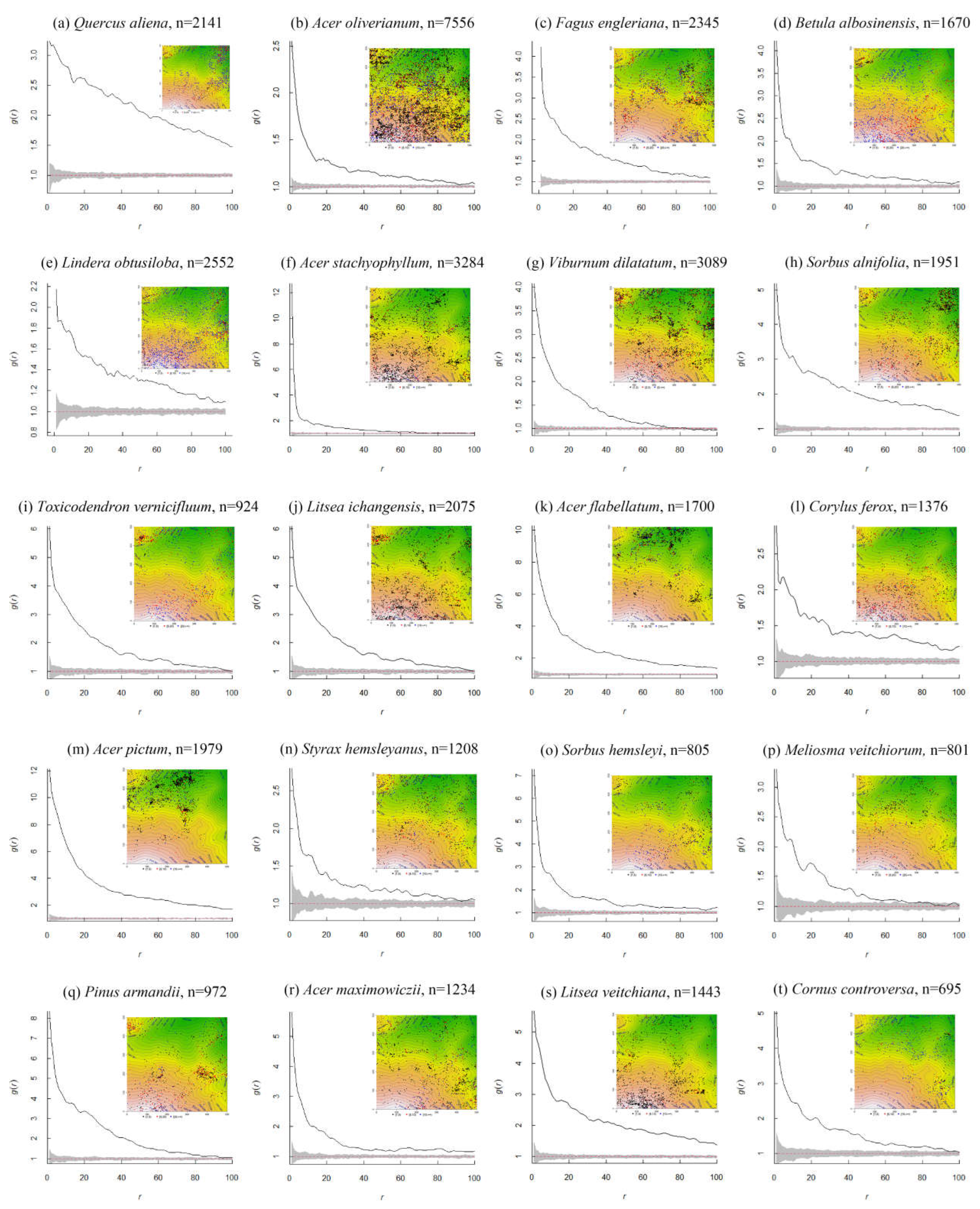

Table 1.
Characteristics of the 20 most dominant woody plants in the 25 ha Shennongjia (SNJ) plot.
| Species name | Family name | Abundance | Basal area (m2/hm2) | Maximum DBH (cm) | Importance value | Life form |
| Quercus aliena var. acutiserrata | Fagaceae | 2141 | 136.12 | 105.92 | 0.0749 | D |
| Acer oliverianum | Sapindaceae | 7556 | 109.66 | 51.80 | 0.0742 | D |
| Fagus engleriana | Fagaceae | 2345 | 95.90 | 83.50 | 0.0663 | D |
| Betula albosinensis | Betulaceae | 1670 | 50.56 | 102.23 | 0.0571 | D |
| Lindera obtusiloba | Lauraceae | 2552 | 50.50 | 59.82 | 0.0455 | D |
| Acer stachyophyllum subsp. betulifolium | Sapindaceae | 3284 | 31.80 | 21.22 | 0.0310 | D |
| Viburnum dilatatum | Adoxaceae | 3089 | 22.93 | 14.45 | 0.0277 | D |
| Sorbus alnifolia | Rosaceae | 1951 | 19.01 | 42.36 | 0.0248 | D |
| Toxicodendron vernicifluum | Anacardiaceae | 924 | 17.27 | 53.60 | 0.0247 | D |
| Litsea ichangensis | Lauraceae | 2075 | 15.08 | 48.11 | 0.0223 | D |
| Acer flabellatum | Sapindaceae | 1700 | 13.45 | 52.56 | 0.0211 | D |
| Corylus ferox var. thibetica | Betulaceae | 1376 | 12.97 | 49.31 | 0.0190 | D |
| Acer pictum subsp. mono | Sapindaceae | 1679 | 12.93 | 47.80 | 0.0190 | D |
| Styrax hemsleyanus | Styracaceae | 1208 | 12.22 | 47.10 | 0.0183 | D |
| Sorbus hemsleyi | Rosaceae | 805 | 11.89 | 92.99 | 0.0176 | D |
| Meliosma veitchiorum | Sabiaceae | 801 | 11.50 | 97.50 | 0.0170 | D |
| Pinus armandii | Pinaceae | 972 | 10.66 | 78.47 | 0.0166 | E |
| Acer maximowiczii | Sapindaceae | 1234 | 10.48 | 32.12 | 0.0164 | D |
| Litsea veitchiana | Lauraceae | 1443 | 10.49 | 20.11 | 0.0163 | D |
| Cornus controversa | Cornaceae | 695 | 9.66 | 49.40 | 0.0158 | D |
Table 2.
Dominant species with more than 200 individuals in each life stages.
| Species name | Layer | Abundance | Individuals of Small Trees | Individuals of Medium Trees | Individuals of Large Trees |
| Quercus aliena var. acutiserrata | Canopy | 2141 | 222 | 718 | 1201 |
| Acer oliverianum | Understory | 7556 | 4613 | 1673 | 1270 |
| Fagus engleriana | Canopy | 2345 | 824 | 899 | 622 |
| Lindera obtusiloba | Understory | 2552 | 368 | 617 | 1567 |
| Viburnum dilatatum | Shrub | 3089 | 1874 | 384 | 231 |
| Acer flabellatum | Understory | 1700 | 1135 | 337 | 228 |
Disclaimer/Publisher’s Note: The statements, opinions and data contained in all publications are solely those of the individual author(s) and contributor(s) and not of MDPI and/or the editor(s). MDPI and/or the editor(s) disclaim responsibility for any injury to people or property resulting from any ideas, methods, instructions or products referred to in the content. |
© 2025 by the authors. Licensee MDPI, Basel, Switzerland. This article is an open access article distributed under the terms and conditions of the Creative Commons Attribution (CC BY) license (https://creativecommons.org/licenses/by/4.0/).
Copyright: This open access article is published under a Creative Commons CC BY 4.0 license, which permit the free download, distribution, and reuse, provided that the author and preprint are cited in any reuse.


