1. introduction
With humans' deepening exploitation of marine resources, the aquatic ecosystem faces increasing pressure (Yu, 2020; Hong and Lin, 2002). The construction of artificial reefs has received widespread attention and application to protect and restore the marine ecosystem. Artificial reefs are structures artificially installed in the ocean that can provide marine organisms with habitat(Farinas-Franco and Roberts, 2014), reproduction, and feeding sites by altering the current flow field(Gatts et al., 2015), thereby promoting the recovery and growth of marine living resources(Chua C. and Chou L.M., 1994; Seaman W J, 2000). The flow field effect of fish reefs is mainly determined by some upwelling and back eddy characteristics, including upwelling and back eddy area, height, etc., which are important indexes to measure the standard of fish reef construction(Yu et al., 2019).
Different types of reefs have various shapes, which have a significant effect on the flow field. A larger surface area can provide sufficient attachment opportunities for seaweeds, thus promoting the formation of seaweed beds, and a complex structure contributes to the formation of turbulence, which has a significant effect on the performance of their fish aggregations(Sherman et al., 2002; Jiang et al., 2014, Liu and Su, 2013). The flow field of artificial reefs varies with different shapes and opening ratios(Li and Zhang, 2010; Kageyama M et al., 1982; Shao et al., 2014; Liu et al., 2011), and a reasonable opening ratio and number of openings will enhance upwellings and back eddies, while an excessive amount will have negative impacts(Fu et al., 2014). For hollow as well as artificial reefs with openings, variations in the permeability coefficient (Wang et al., 2018) affect the flow conditions of artificial reefs. Different incoming flow velocities and headwater angles can significantly affect the flow field effects of artificial reefs(Zheng et al., 2012), with the magnitude of the incoming flow velocity determining the magnitude of the impact and shear forces of the current on the reefs (Zhang et al., 2020), while the headwater angle determines the relative direction of the current for the reefs and the area of action (Jiang et al., 2019).
Currently, scholars at home and abroad have conducted many studies on the flow field effects of artificial reefs. These studies have mainly used numerical simulations (Guan et al., 2016; Lu et al., 2006) and physical model tests (Fu, 2013; Liu, 2021). Numerical simulation methods can quickly and accurately predict the flow field effects of artificial reefs. Still, they require reasonable simplifications and assumptions about the computational model, so the reliability of their results needs to be verified by physical model tests(Kim D et al., 2021). In previous studies, most scholars focused only on the flow field effects of single-type and functional artificial reefs at specific incoming flow velocities and incoming flow angles.
The main economic products of the area of South Sulawesi Province are seaweeds and groupers, as well as small-scale shrimps, shellfish, sea cucumbers, etc. Groupers are coral reef-type fishes (La Ode et al.,2015) and are suitable to inhabit coral reef crevices, and coral reefs provide a rich source of subsistence for groupers(Afero, F et al., 2010; Albasri, H et al., 2010). Coral reefs are home to various marine organisms, including algae, shellfish, shrimp, and crabs, which provide rich food options for grouper(Aslan, L.O.M., 2008). The complex structure of artificial reefs provides hiding places and breeding grounds for grouper, which is conducive to the survival and growth of grouper(X. Moreno-Sánchez et al., 2019). Three kinds of artificial reefs have been designed with different structures and functions according to the living habits of major fish species and the ecological environment of the seabed to achieve the purpose of aquaculture and restoration of the marine environment.
In this paper, three types of artificial reefs with different design objectives are combined with numerical simulation and physical model test to study the current field effect of these three types of artificial reefs under different incoming current speeds and current angles, analyze the influence of the incoming current speed, current angle, shape and structure of the reefs on the current field effect, explore and verify the scale and functionality of the current field after the proposed release, and provide scientific bases for the design of the artificial reefs and the influencing factors. It will also provide a scientific basis for the design of artificial reefs and the factors affecting them, and at the same time, provide technical support for the protection of marine ecology and the sustainable use of aquatic resources.
2. Material and Methods
2.1. Reef Model
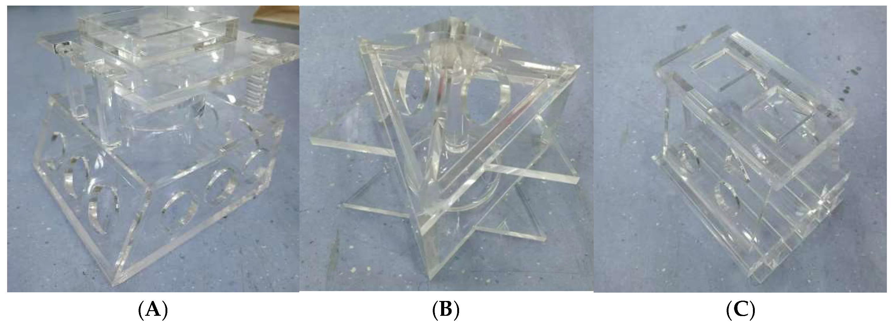
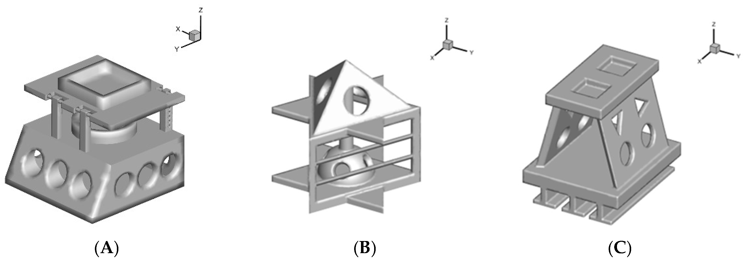
The simulation model with Solidwork designed three kinds of fish reefs, such as in
Figure 1, the size of the reef model A is 3m (L) × 3m (W) × 3m (H), mainly for juvenile fish, the lower hollow side is open with holes to provide an ideal habitat for juvenile fish, and at the same time to simulate the shrimp in the natural environment of the habitat to provide food for the juvenile fish, the internal space allows juvenile fish to escape from the enemy. The upper and top layers are equipped with grooves to allow algae and shellfish to attach; Model B is in the shape of a hexagram, with dimensions of 3m (L) x 2.7m (W) x 3m (H), targeting juvenile and sub-adult fish, which enter the sub-adult stage and increase in size and mobility. The structure of the frame can change the local water flow, making it easier for plankton to gather around the reef, and the gaps and channels between them can allow sub-adult fish to weave in and out of them and are sufficient to provide shelter space; Model C measures 3m (L) x 2.7m (W) x 3m (H) and is mainly aimed at adult fish, which have a larger size and is fitted with a removable base at the bottom to prevent sinking. The reef has ample hollow space to provide a more expansive habitat for adult fish, and a groove is opened at the top to attach various algae and shellfish.
2.2. PIV Test
The test model was scaled down to a modeling size of 1:15, the material was Plexiglas, and the model parameters are shown in
Table 1.
Figure 2.
Life-size model.
Figure 2.
Life-size model.
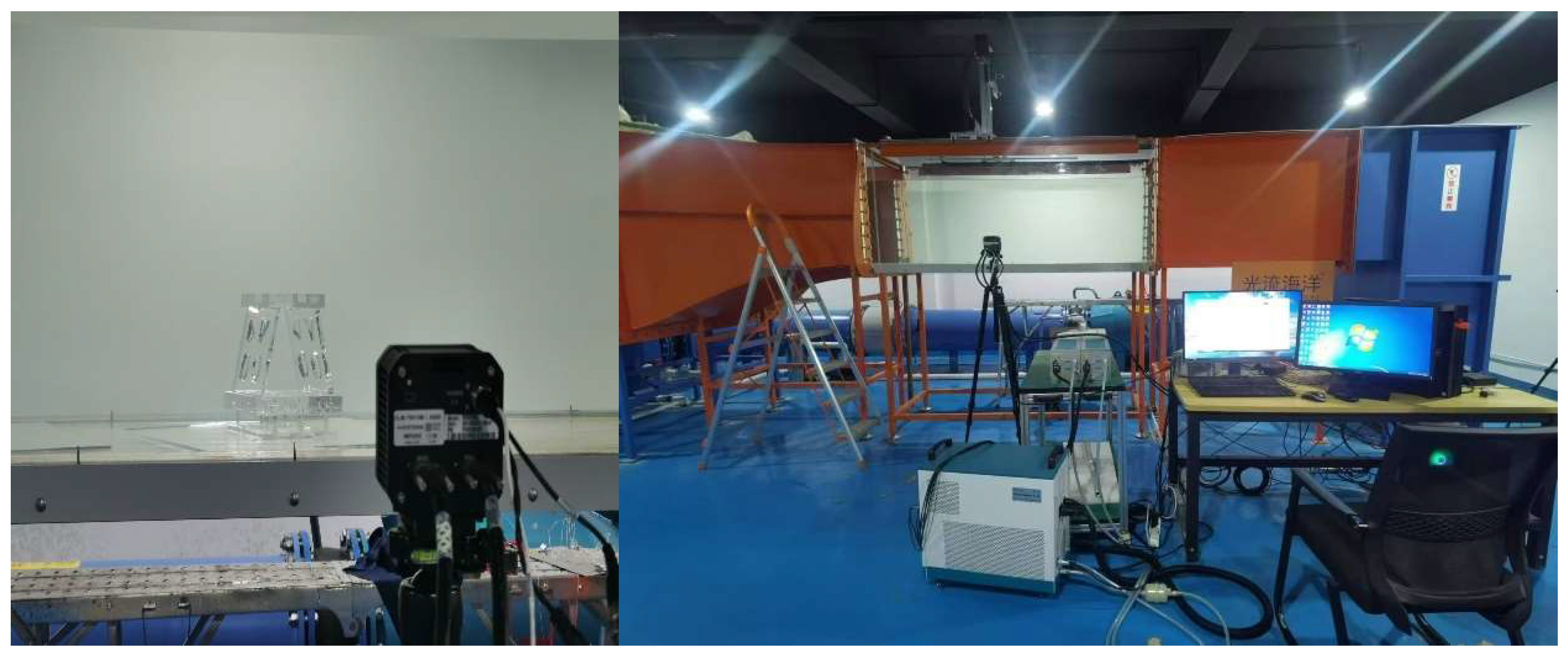
The flume test was carried out in a hydrodynamic circulation tank, as shown in
Figure 3. The size of the flume test section is 200 cm × 80 cm × 70 cm (L × W × H), and the maximum flow rate can be up to 1 m/s. It is also equipped with a data acquisition instrument, a high-speed camera, a laser, and a PIV particle velocimeter. The fish reef model is fixed in the test section. The origin is located in the center of the reef body bottom point, along the current direction for the x-axis positive (flow direction), vertical current direction up for the y-axis positive (lateral), to establish a three-dimensional coordinate system. The flow field in the x-y center-axis plane of the reef was measured using PIV during the test.
1) Place the fish reef model at 0°, 15°, 30° and 45° to the flow angle, set the target flow velocity, and turn on the flow-making device;
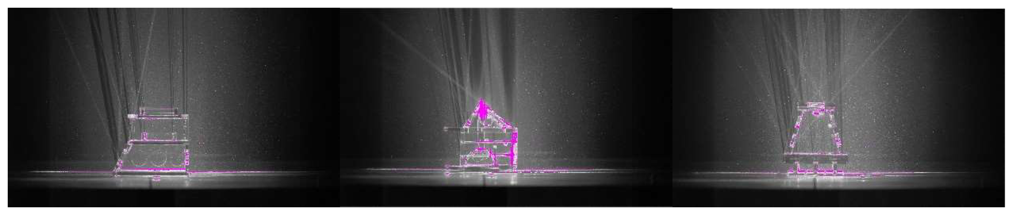
2) After the flow velocity was stabilized, a high-speed camera was used to take pictures and collect image data, see
Figure 4.
3) The obtained particle images are first imported into PIVlab for processing, and the transient flow field map is obtained by selecting the image region to be analyzed for image correction, image analysis, error vector rejection, and data smoothing.
4) The data processed by PIVlab were imported into Tecplot software for further detailed processing and analysis.
Figure 3.
Model fixation and PIV instrumentation.
Figure 3.
Model fixation and PIV instrumentation.
Figure 4.
Capture particle images.
Figure 4.
Capture particle images.
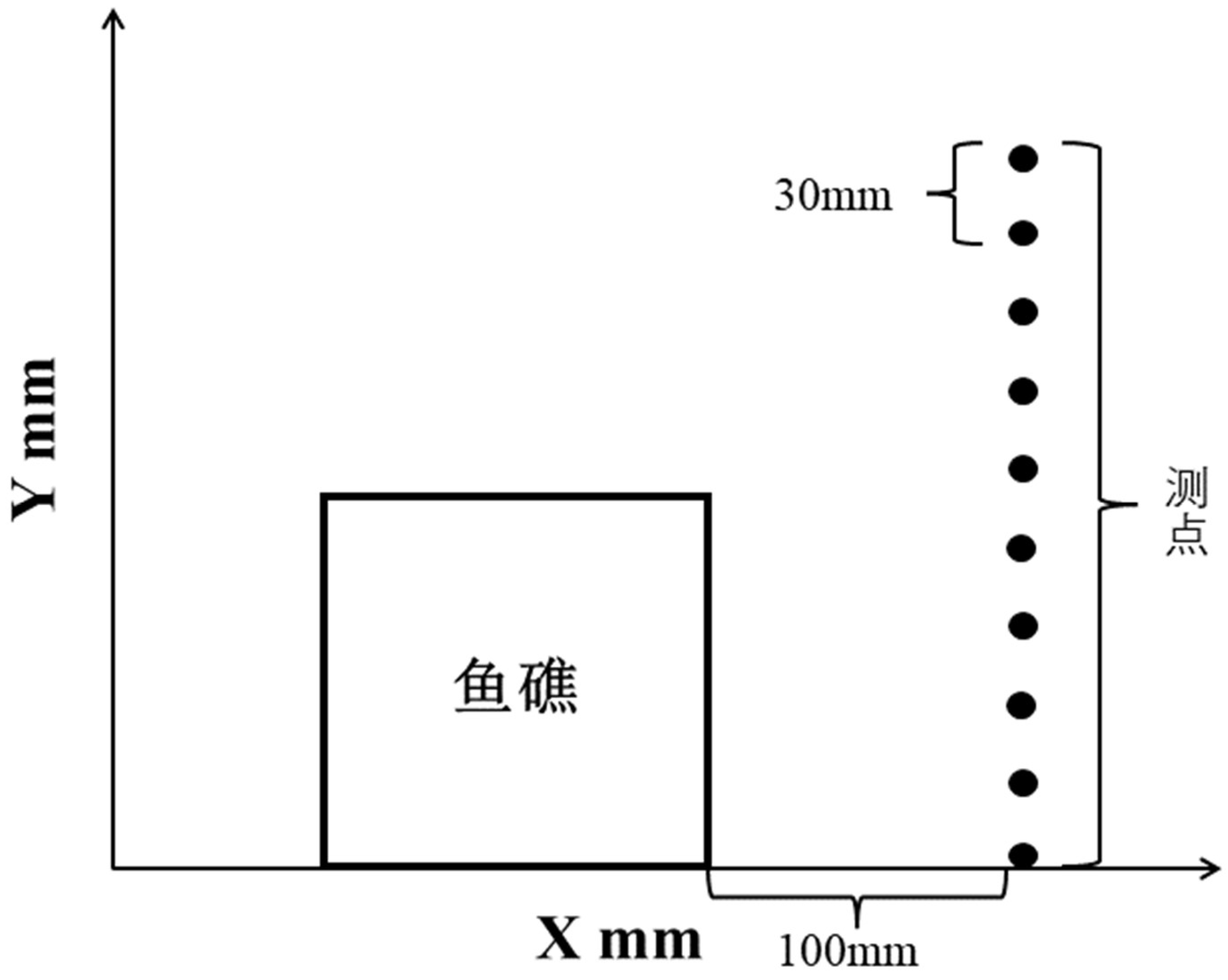
Figure 5.
Measurement point location.
Figure 5.
Measurement point location.
2.3. Numerical Simulation Methods
2.3.1. Governing Equations
In this paper, we adopt the RNG k-ε turbulence model, whose basic idea is to regard turbulence as a transport process driven by random forces, eliminate its small-scale eddies by spectral analysis, and merge their effects into vortex viscosity (Lu et al., 2006), compared with the standard k-ε turbulence model, the RNG k-ε turbulence model has the following characteristics The most important feature of the RNG k-ε turbulence model is that:
1) The rotational and cyclonic flow cases in the mean flow are taken into account by correcting the turbulent viscosity;
2) An additional coefficient C1 is calculated in the ε equation, thus reflecting the time-averaged strain rate Si,j of the main flow, such that the resulting term in the RNG k-ε model is not only related to the flow situation but also a function of the spatial coordinates in the same problem.
Thus, the RNG k-ε model can better handle flows with high strain rates and a significant degree of streamlined bending and respond better to transient flows and streamlined bending effects than the standard k-ε model. The k and ε equations for the RNG k-ε model are as follows:
Where: is the turbulent viscosity; and are the adequate Trump numbers; is the effective viscosity coefficient.
The basic equations of the numerical model of the artificial reef hydrodynamics are the continuum equations with the N-S equations for viscous incompressible fluids without considering the variation of the fluid density:
Where: : fluid density, kg/m3; : the average flow rate of X, Y, and Z directions under the spatial coordinate system after filtration, m/s;: the average pressure after filtration, Pa; μ: is the kinetic viscosity, Pas;: the sub-lattice stress, expressed as follows: .
2.3.2. Computational Domain and Boundary Conditions
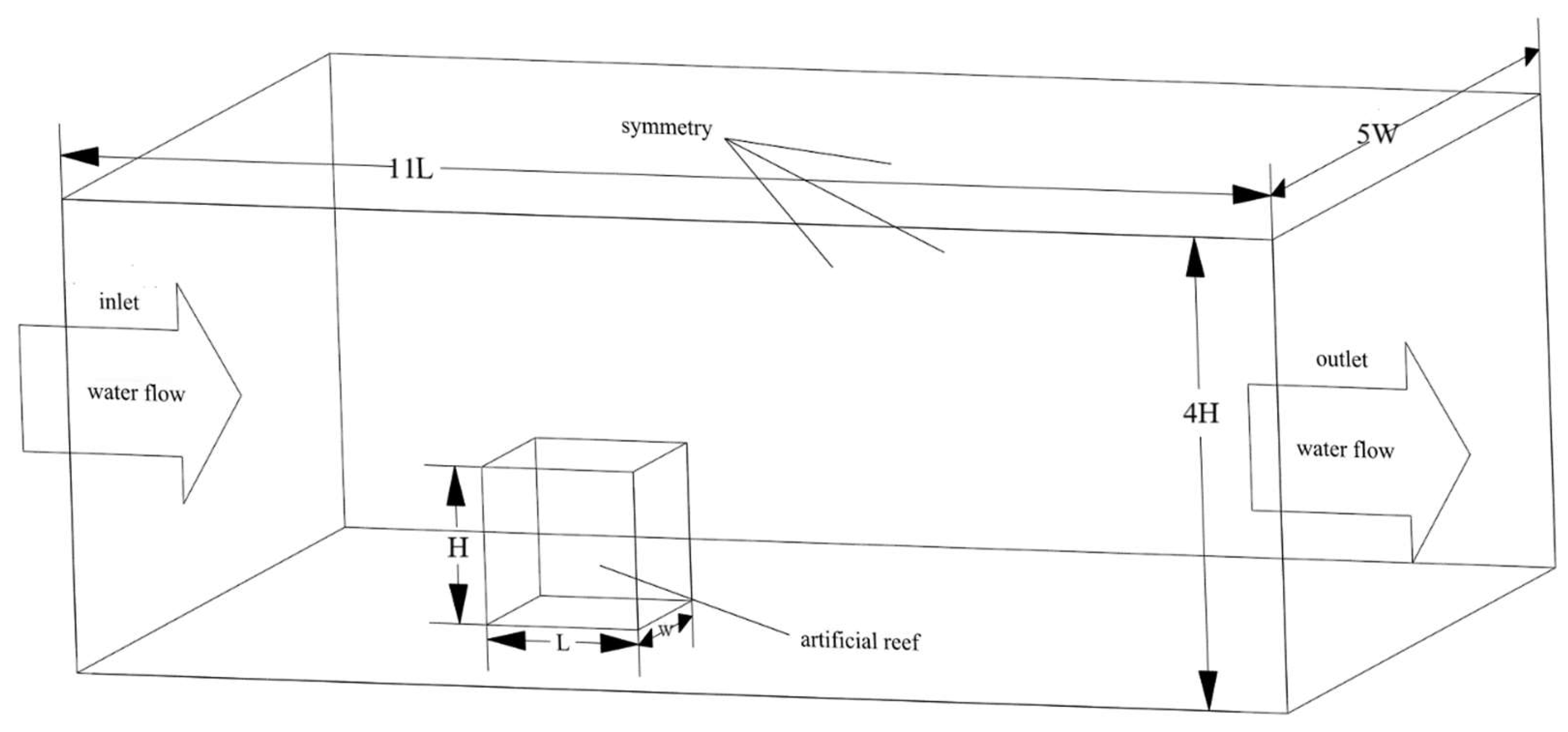
The computational domain of the flow field in this study includes inlet boundary, outlet boundary, symmetry boundary, and wall boundary, and the computational domain is set to be 3 times the reef length in front of the reef, 7 times the reef length in the back, 5 times the reef width in width, and 3 times the maximum height of the reef in height, as shown in
Figure 6.
Figure 6.
Numerical simulation computational domain.
Figure 6.
Numerical simulation computational domain.
The following settings are made for the boundary conditions:
1) The inlet boundary condition is a velocity inlet. The corresponding incoming velocity is set, and the turbulence intensity and turbulent viscosity ratio on the boundary are calculated and given;
2) The outlet boundary is a pressure outlet;
3) The bottom surface of the computational domain, the side walls, and the surface of the artificial reef body are set as wall boundary conditions, and the standard wall boundary parameters of static no-slip are used.
In the simulation, the fluid density is set as the typical density of seawater 1024 kg/m³, and the second interpolation (QUICK) approximation is chosen for spatial discretization; the equations are iterated to the steady state by SIMPLEC for velocity-pressure correction; and it is assumed that the residuals are lower than 10-5 when convergence is achieved. Considering the influence of storm surge and extreme weather, the current speed may be increased to make the experimental results more obvious, so the experimental incoming currents are selected to be 0.2 m/s, 0.4 m/s, 0.6 m/s, 0.8 m/s, and 1.0 m/s, and four current angles, namely, 0°, 15°, 30°, and 45°, are chosen to investigate the effects of different current speeds on the flow fields of three different reefs.
2.3.3. Meshing
Grids are divided to consider the accuracy of computation on the one hand and the efficiency of calculation on the other. Currently, grids can be roughly divided into two categories: structured grids and unstructured grids. As shown in
Table 2, the respective advantages and disadvantages of structured and unstructured grids are listed.
In order to ensure that the simulation results under the premise of effectively improving the speed of calculation, according to the reef and the characteristics of the computational domain are entirely symmetrical, the symmetry analysis method is used, the numerical calculations, assuming that the origin of the coordinates is located in the center of the bottom surface of the reef, the direction of the incoming flow is along the direction of the X-axis, the Y-axis is the vertical direction, and Z = 0 in the pendant plane (XOY plane) is selected as the middle pendant plane of the study. The simulation model of the reef was created using Solidworks software and imported into the computational domain established by the ANSYS Workbench Mesh module. The area is meshed with tetrahedral unstructured mesh, the size of the flow field area is 0.1m, the surface of the fish reef ranges from 0.045 to 0.09m in size as required, the growth rate is 1.1, and the number of meshes of the fish reef model is finally in the range of 1×10⁷ to 1×10⁸.
2.3.4. Selection of Indicators for the Flow Field Region
The scaled index of the flow field effect of artificial reefs is an evaluation factor used to indicate the impact of the flow field of artificial reefs. The effect of the flow field is mainly generated by the upwelling on the facing surface and the back eddy on the back surface. When the flow velocity reaches a specific value, the corresponding flow field movement will produce the corresponding functional effects. Hence, the speed index is the selected standard of the upwelling and back eddy area. For this reason, the upwelling zone was chosen as the velocity region where the vertical flow velocity at the front of the reef was more incredible than 10% of the incoming flow velocity. The back eddy zone was the velocity region where the absolute value of the incoming flow velocity at the back of the unit reef was less than 80% of the incoming flow velocity(Gou, 2020).
3. Results
3.1. Test Results
3.1.1. Characterization of Flow Patterns in the Mid-Axial Plane
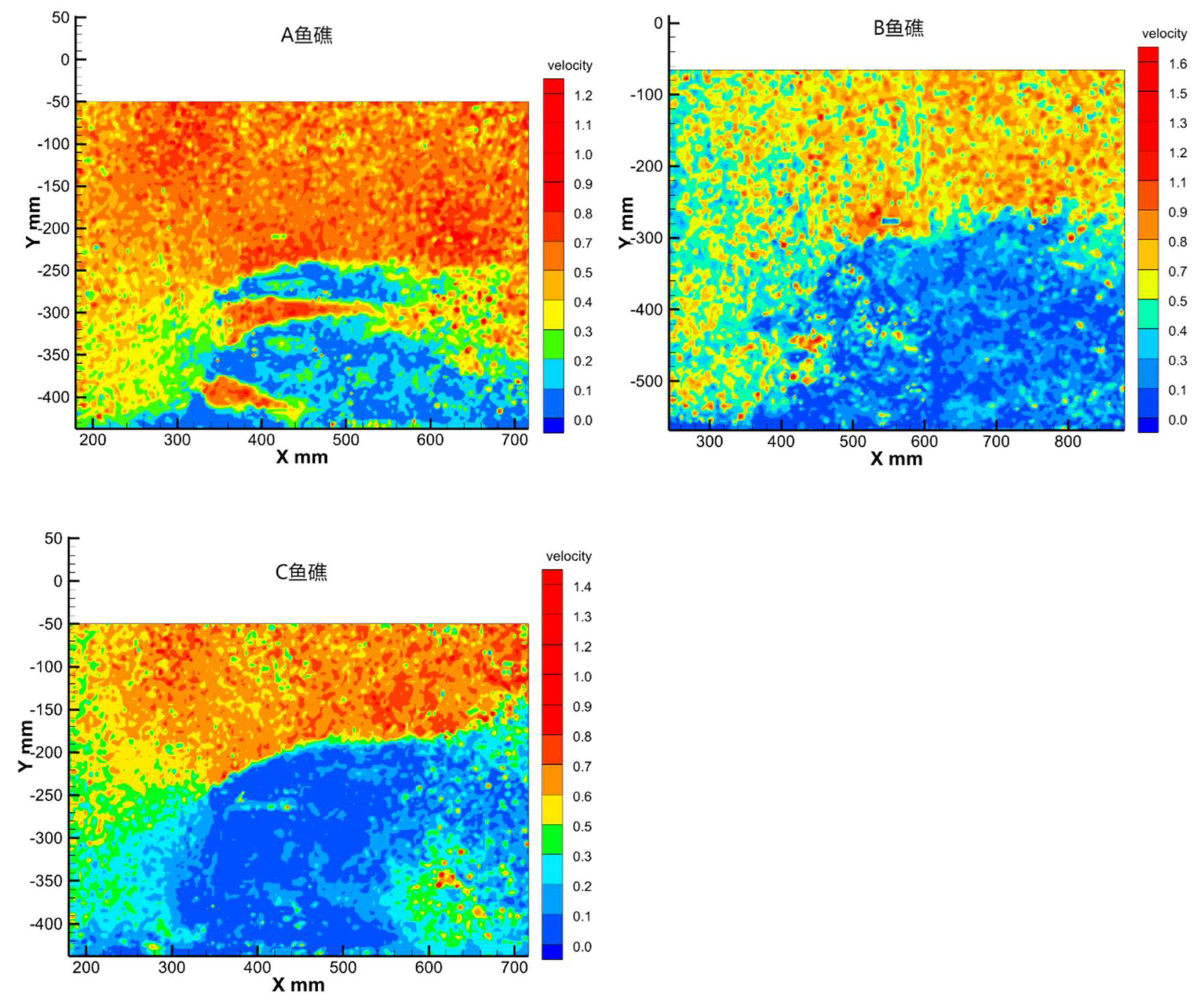
As shown in
Figure 7 and
Figure 8, the flow conditions of the axial surface particles in the three types of artificial reefs are compared when the angle of the headward current is 0° and v = 0.5 m/s. From the figure, it can be seen that all three types of artificial reefs form a specific scale of upwelling above them. The upwelling areas of A and C are more extensive, and a small portion of the slow flow area is generated within 50 mm above the reef. Among them, the cavity structure of Reef A has a noticeable gap pipe flow effect inside the reef.
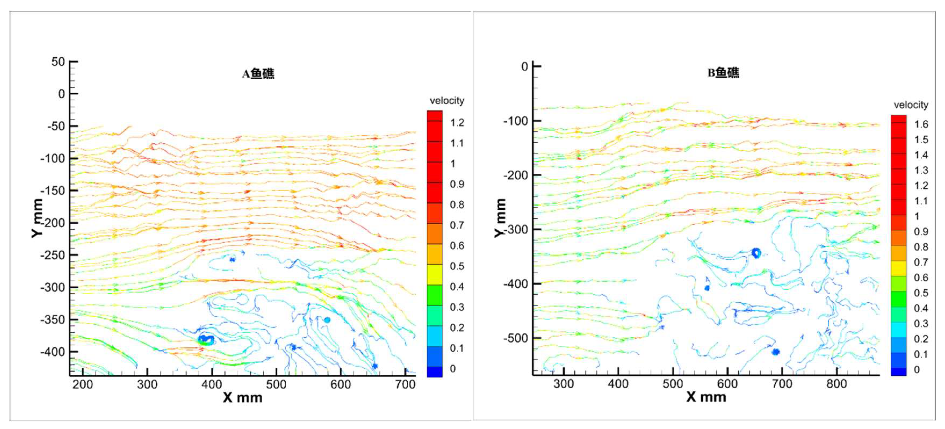
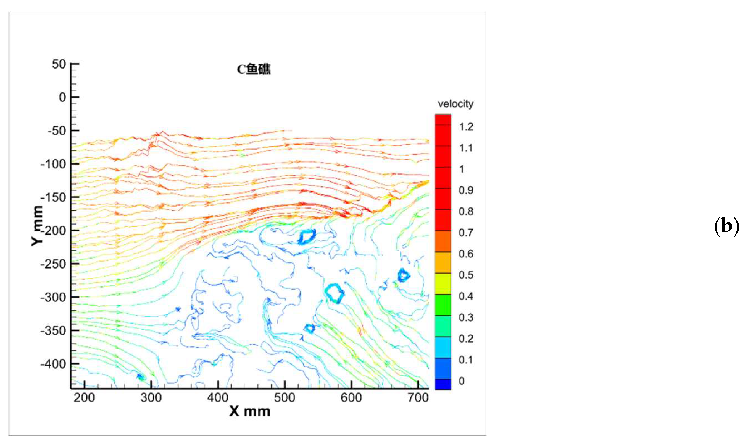
Meanwhile, the upwelling area of Reef B is smaller, and the inclination angle of the flow-facing surface is smaller. On the contrary, Reef B and C have larger back eddy areas, and Reef A reduces the scale of the back eddy behind the reef due to its internal cavity structure. Velocity vector plots show that all three types of reefs have significant eddy generation behind the reefs. In the wake behind Reef C, a part of the current touches the bottom to form an upwelling with an increased velocity. There is also a significant acceleration of the current at the inner void of Reef A and small areas of eddy disturbance at and around the inner structure of Reef B and C.
Figure 7.
Velocity cloud map of the center axis surface.
Figure 7.
Velocity cloud map of the center axis surface.
Figure 8.
Vector diagram of center-axis surface velocity.
Figure 8.
Vector diagram of center-axis surface velocity.
3.1.2. Point Velocity Results
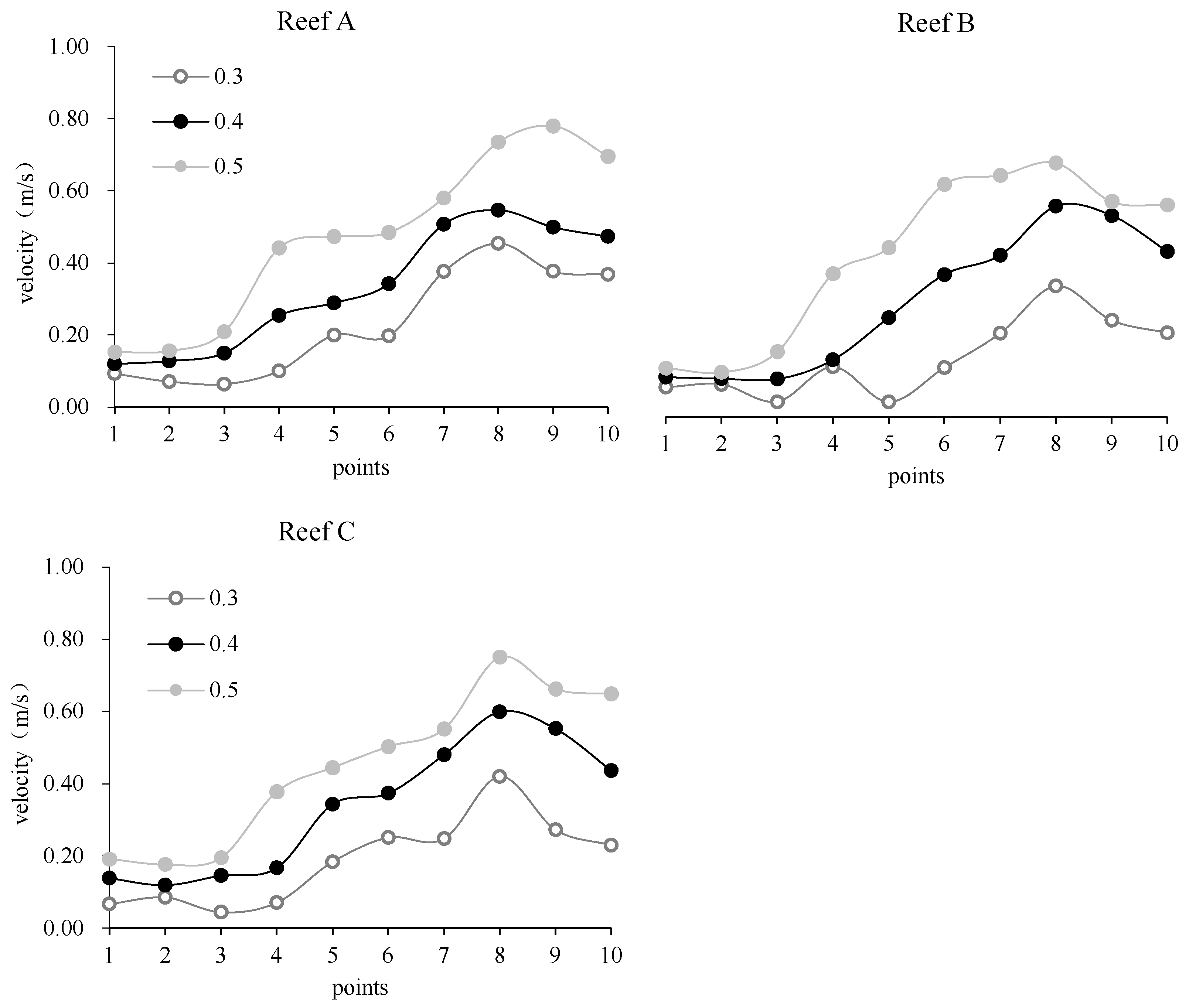
As shown in
Figure 9, the flow velocities at each reef are compared and analyzed at three headwater velocities at 0° headwater angle. The figure shows that with the increase of the headward current velocity, the flow velocity of all the measurement points of the three types of Reef A, B, and C increases, of which the first four measurement points have minor changes, i.e., the flow velocity in the back eddy area behind the reefs has minor changes. After measurement point 6, i.e., the upwelling area has significant changes. Overall, the velocity of the three types of reefs behind Reef A, B, and C tends to increase first and then decrease.
3.2. Numerical Results
3.2.1. Cross-Sectional Flow Characteristics
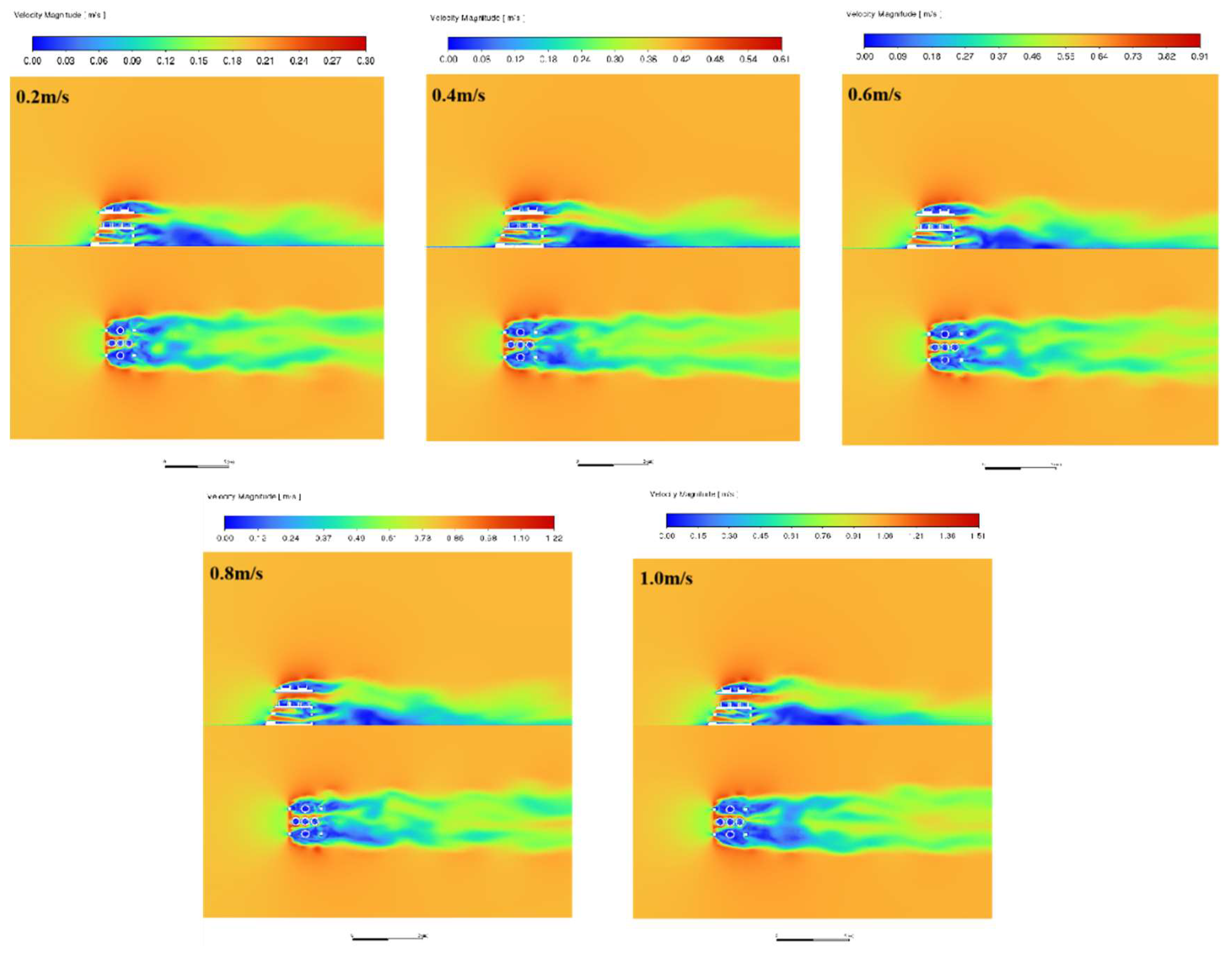
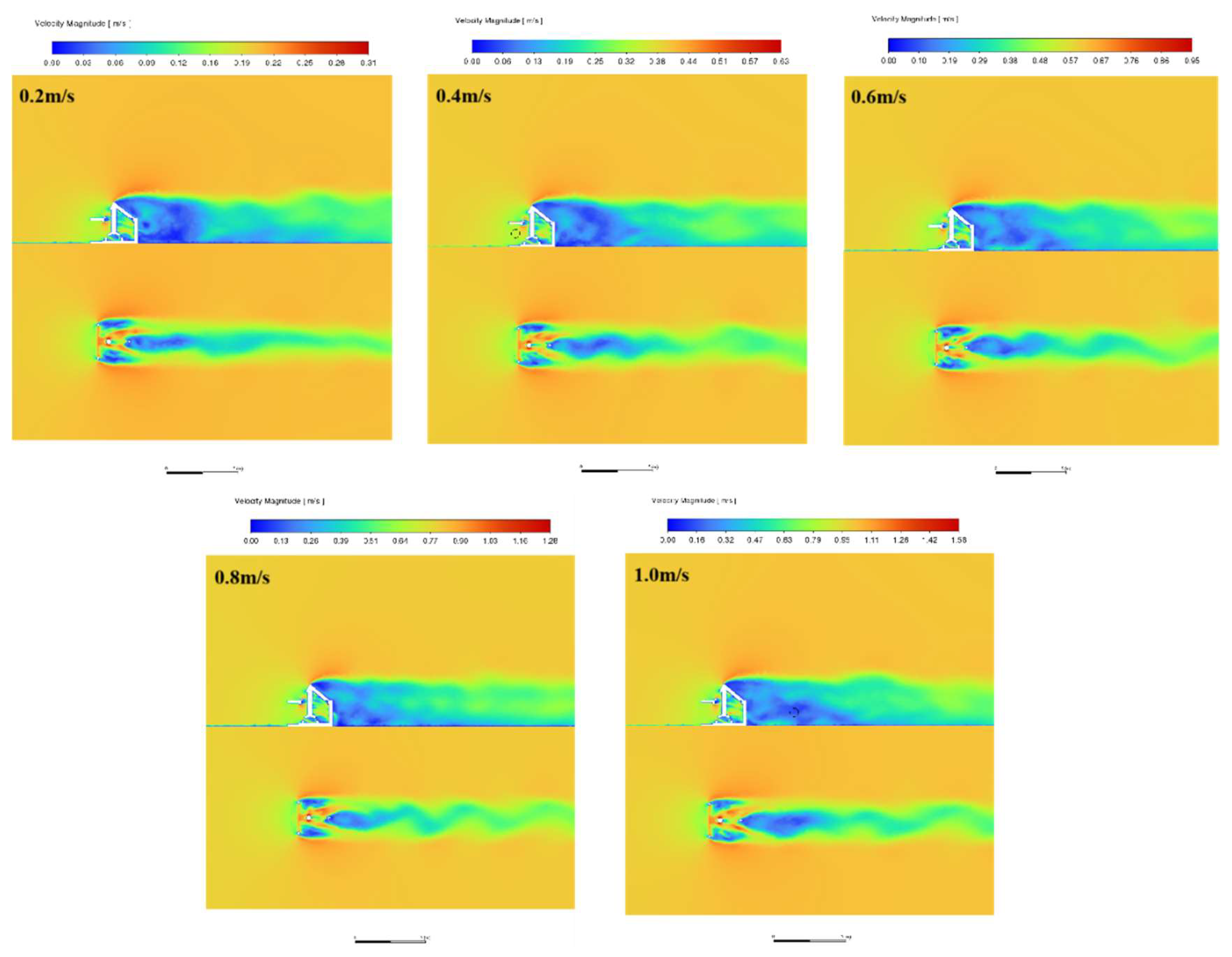
Figure 10,
Figure 11 and
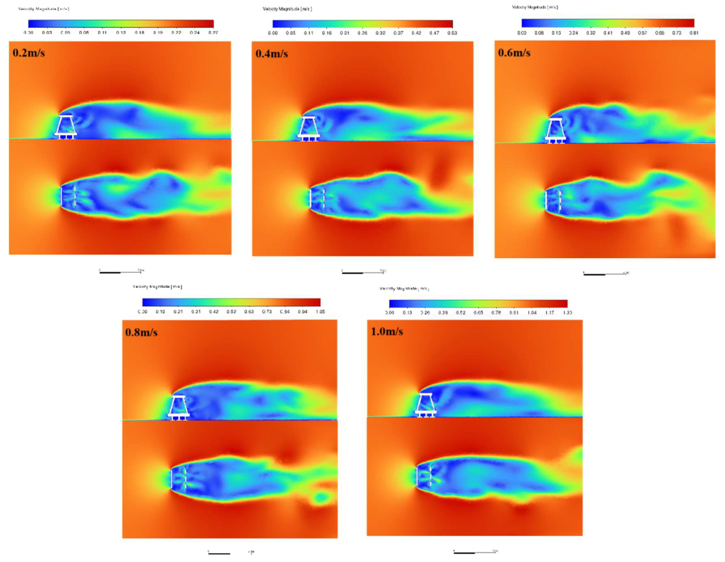
Figure 12 compare the flow conditions in the axial plane (x=1.5m) and cross-section (y=H/2) of the three artificial reefs A, B, and C for different incoming flow velocities at a headwater angle of 0°.
When the incoming flow contacts the reef body, due to the water flow contacting the reef body's headward surface, the ascending effect at the top of the reef produces a significant speed-up phenomenon and a certain amount of upwelling. Reef A center cavity, due to the gap tube flow effect, the flow velocity accelerated to reach the maximum velocity in the flow field area in the cavity with a baffle groove area to form a slow flow area. When the water flow passes through the reef area, the flow velocity shows a significant slowdown due to the increased contact volume of the water flow with the flow field area, reflecting the hindering effect of the fish reef on the incoming flow and generating a backflow area behind the fish reef to form a back vortex flow area. Due to the fewer openings in Reef C, the area of the oncoming flow is relatively larger, showing a good obstruction effect and generating a good eddy effect behind the reef. The upwelling and back eddy areas are significantly larger than those of the remaining two groups of fish reefs. Reefs A, B, and C have more and larger open holes. The voids divert the more the flow surface of the reef body, the weaker the upwelling on the upper side of the reef body, but the tube flow effect inside the reef body is more apparent, and the slow flow area is more. Reef A has a more extended wake with the increase of velocity, the area of the back eddy has increased, and from the cross-section, it can be seen that there is a clear diversion of the flow after the flow passes through the back of the reef body. A fuzzy vortex is generated on both sides and as the flow velocity increases, Reef B has an increased wake, accompanied by a rise in velocity. The Karman eddy behind the reef body has a good effect. The upwelling and back eddy area is significantly larger than the remaining two groups. The Karman vortex phenomenon behind the reef is more prominent, as Reef A's upwelling and back eddy have a larger area than the remaining two reefs.
Figure 13,
Figure 14 and
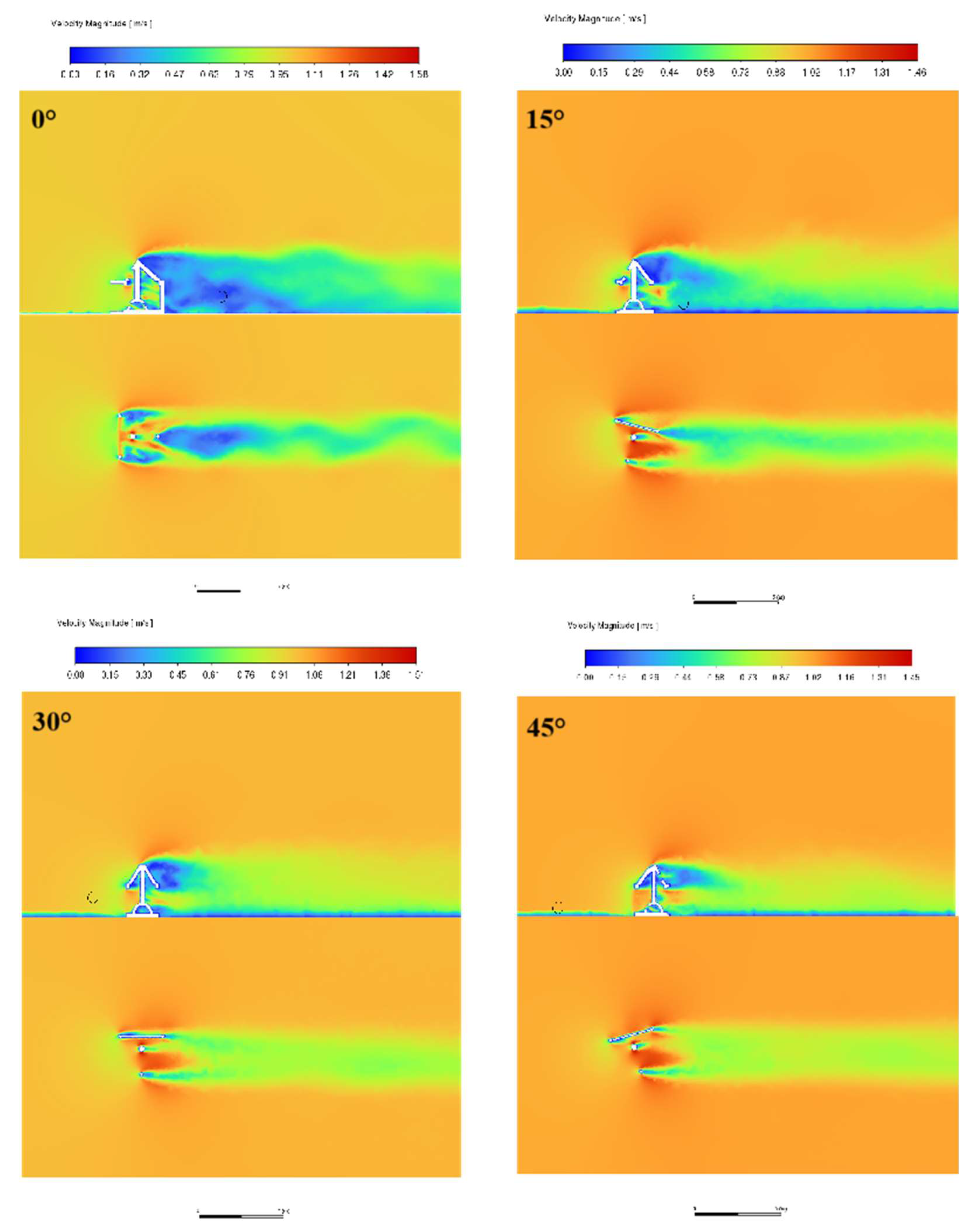
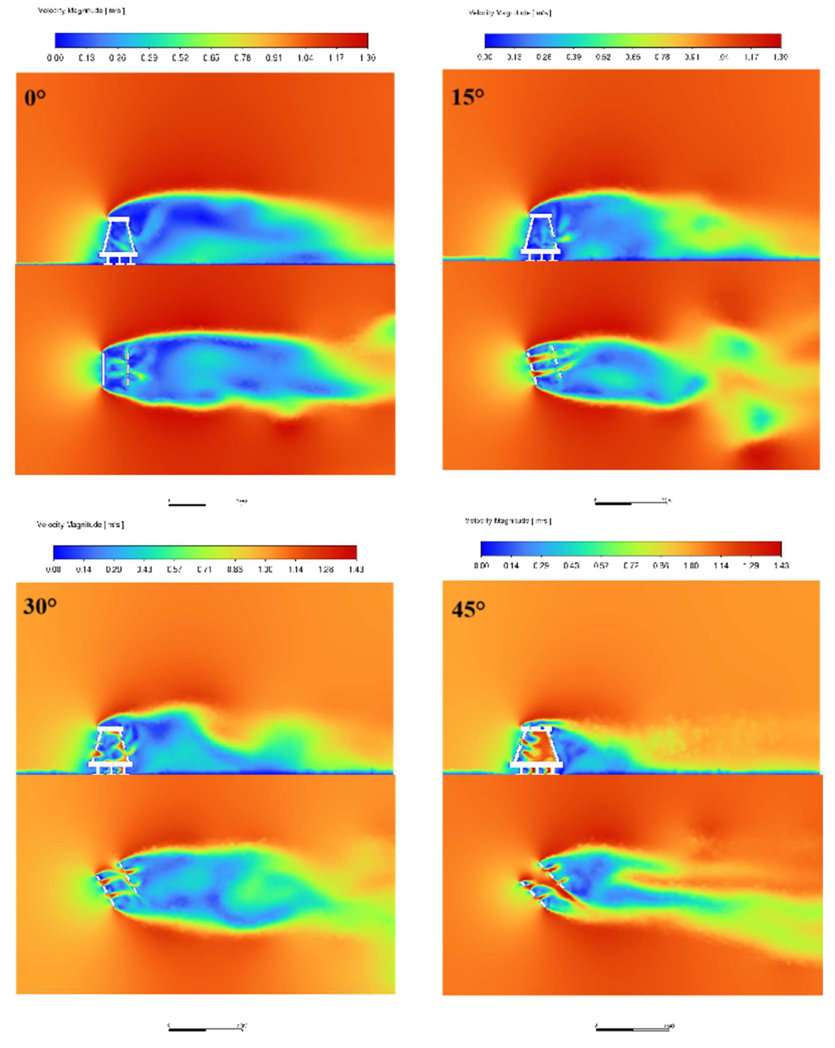
Figure 15 compare the flow regimes in the axial plane (x=1.5m) and cross-section (y=H/2) of the three artificial reefs A, B, and C at v=1.0m/s for different headwater angles.
Under different flow angles, the flow pattern inside the reef and the basin changes significantly due to the surface change. a. Reef A has a more obvious Karman vortex on the left side at 15°, and the larger the angle is, the more pronounced the diversion phenomenon and the wake becomes shorter, the area of the back eddy decreases, and the tube flow effect inside the reef disappears gradually. Reef B has the disappearance of the Karman vortex with the increase of the angle, the back eddy area decreases, and there is a tube flow phenomenon in the reef. Reef C also showed a decrease in the area of the back vortex as the angle increased, a divergence of the flow behind the reef at 45°, and a tube flow effect in the internal structure.
3.2.2. Volume Characteristics of the Flow Field for Different Incoming Velocities
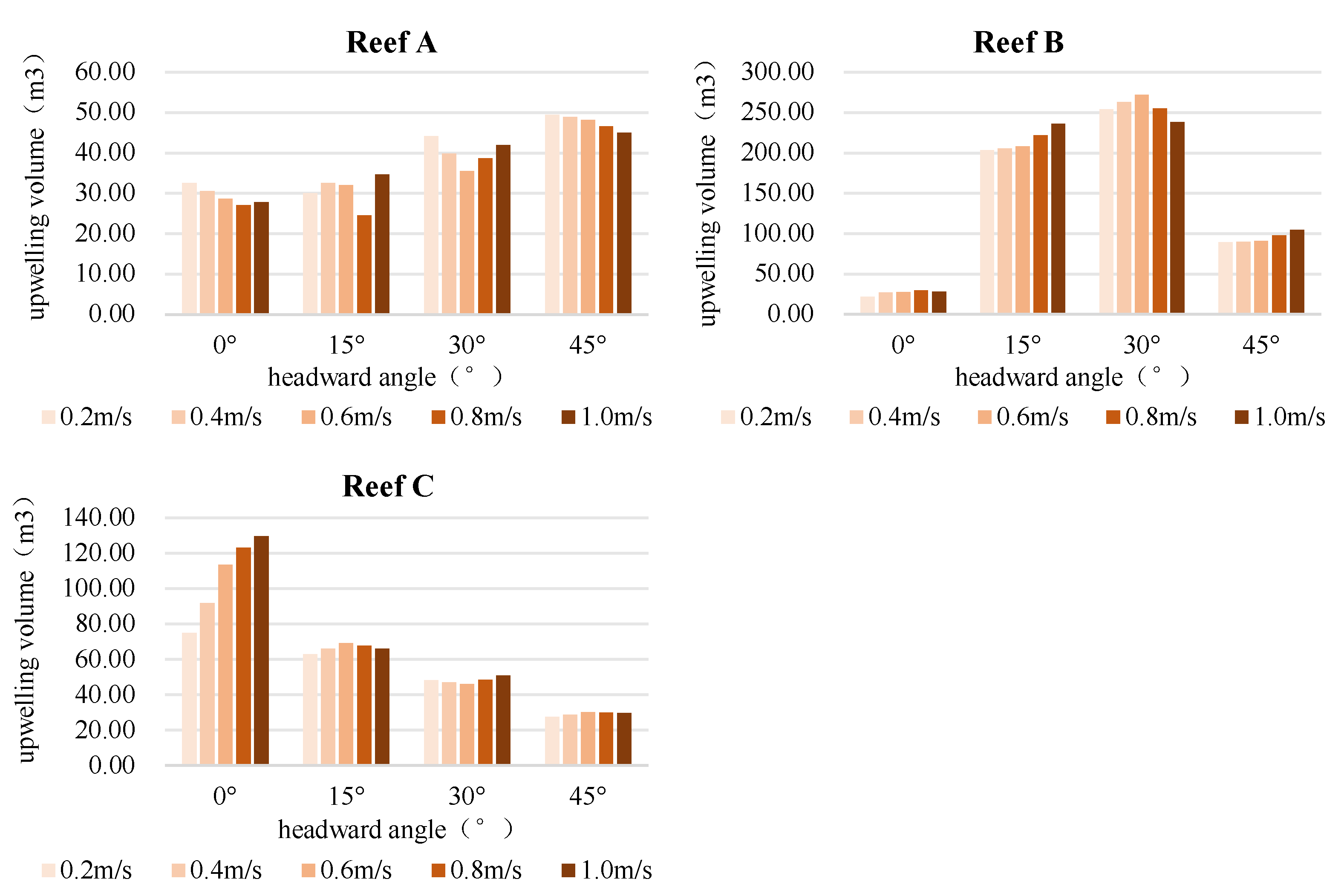
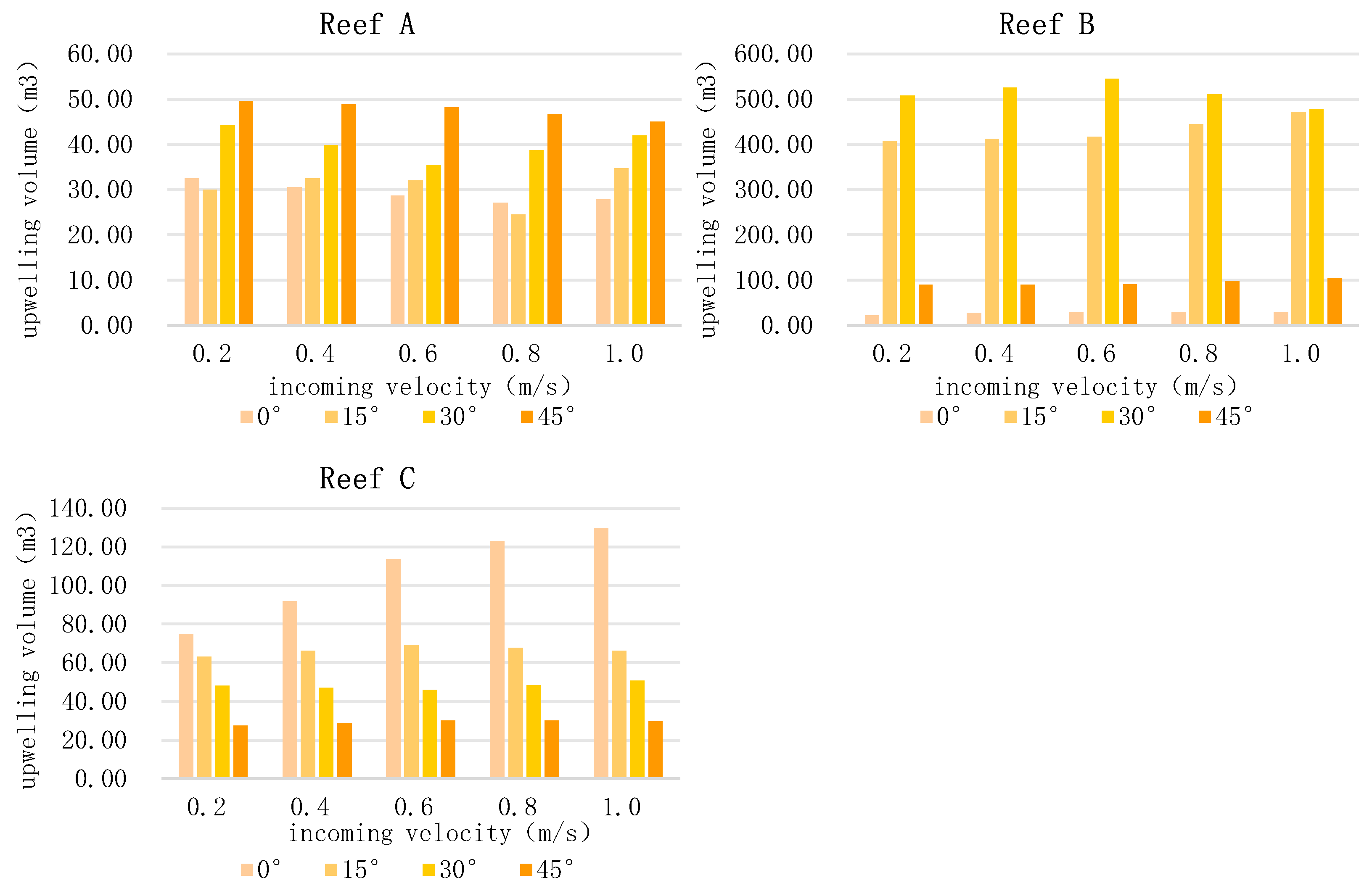
As shown in
Figure 16 on six different artificial reefs with varying angles of flow and changes in flow velocity and the impact on the upwelling, take the incoming velocities 0.2m/s, 0.4m/s, 0.6 m/s, 0.8m/s, 1.0 m/s as a comparative analysis. Reef A upwelling volume in the angle of 0 ° and 45 ° when the volume of the flow velocity increases and decreases, but the change is not significant, the 30 ° when the first decrease and then increases to reach a minimum at v = 0.6m/s, 15 ° no considerable change. The volume of the upwelling of fish reef B did not change significantly with velocity at 0° and 45° but increased with velocity at 15°, then increased and then decreased at 30°, and reached a maximum at v=0.6 m/s. The volume of the upwelling of fish reef C increased with the velocity at 0° and 30°, respectively, and did not change significantly at the other angles.
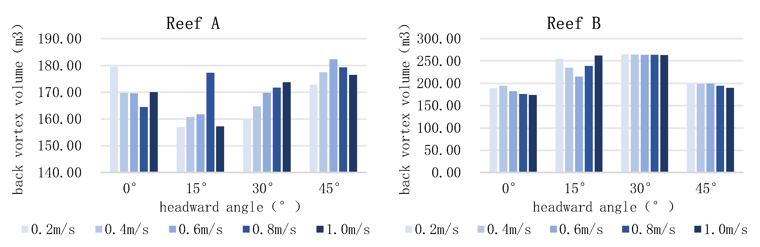
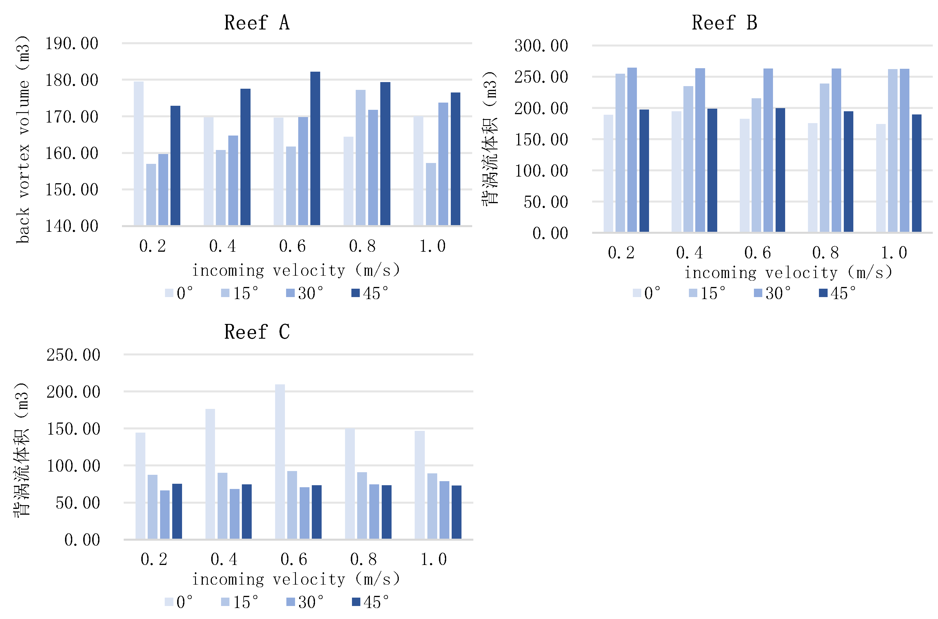
As shown in
Figure 17, for six different artificial reefs with varying angles of headwater, the back eddy is affected by the flow velocity change. Reef A at 15° and 45°, the volume of the back eddy increases with the increase of velocity. It reaches the maximum at v=0.8m/s at 15°, and v=0.6m/s at 45°, and decreases and then increases at 0°, and reaches the minimum at v=0.8m/s, and decreases with the increase of velocity and the decrease of volume at 30°. Reef B decreases and then increases at 15°, reaches a minimum at v=0.6m/s, and there is no clear pattern of change with velocity at other angles. Reef C increases and then decreases at 0°, reaches a maximum at v=0.6m/s, and there is no clear pattern of change with velocity at other angles.
3.2.3. Cross-Sectional Flow Characteristics
The effects of changes in the flow angle on the upwelling of three different artificial reefs at different incoming velocities are shown in
Figure 18. Reef A upwelling volume decreases and then increases with the increase of the flow angle at v=0.2m/s and v=0.8m/s. Both are the smallest at 15° and increase with the flow angle increase at the other velocities. The volume of Reef A increases and then decreases with the increase of flow angle, and is much larger than the rest of the angles at 15° and 30°, and reaches the maximum at 30°. Reef A decreases with the increase of flow angle.
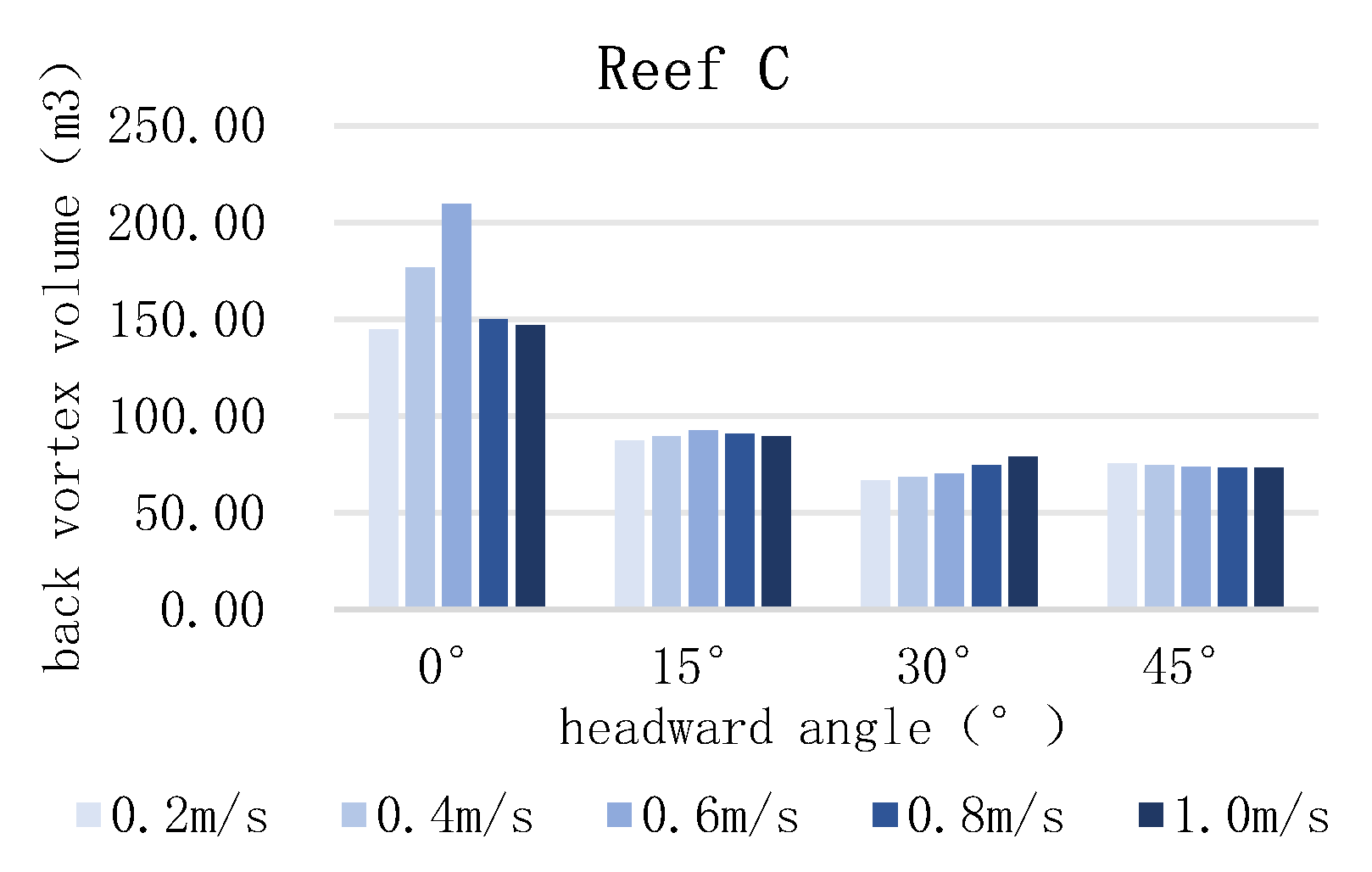
The effects of changes in the angle of flow on back eddy currents at different incoming velocities for six different artificial reefs are shown in
Figure 19. The volume of back eddy currents on reef A decreases and then increases with increasing flow angle and is minimized at 15°. The volume of back eddy currents on reef B increases and decreases with increasing flow angle, reaching a maximum of 30°. The volume of back eddy currents on reef C is much larger at 0° than at the other three angles, and the difference in volume of back eddy currents is relatively tiny in the different angles. Reef A has a much larger back eddy volume at 0° than the other three angles, and the difference in back eddy volume at other angles is slight.
3.3. Validation of Results
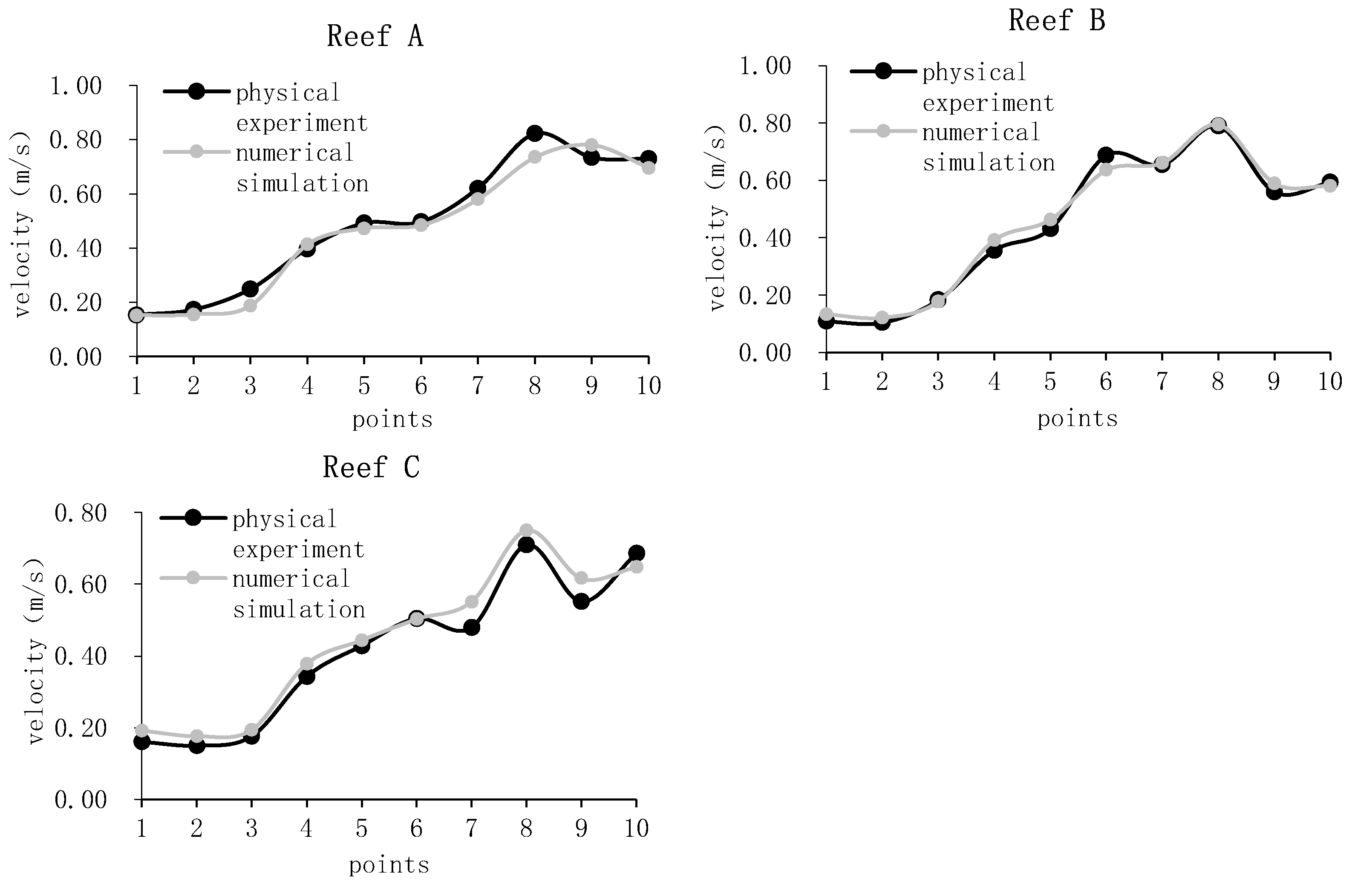
Validation experiments using cross-sectional measurement of the control point method, the computational domain, and the numerical model will be reduced by 15 times following the same numerical simulation method, taking the exact location of the measurement point, the flow velocity of the measurement point of the physical experiments against the numerical simulation of the flow velocity comparison, the specific area of the measurement point is shown in
Figure 20, used to respond to the effect of the back vortex at the back of the reef as well as the trend of the upper updrafts.
Comparison of the flow velocity at different flow measurement points of the flume experiment and numerical simulation, as shown in
Figure 20, the comparison of the velocity at the measurement points of the flume experiment and numerical simulation post-processing data, the trend of change is the same. After calculation, the relative errors of the six types of reefs are 1.00%~24.74%, 0.66%~22.51%, 0.38%~18.69%, and the average errors are 7.43%, 7.52%, and 9.86%.
4. Discussion
The incoming current velocity changes affect different reefs' upwelling and back-eddy volumes. For example, the upwelling volume of the reef at 0° for Reef C shows a gradual increase with increasing incoming velocity (Liu et al., 2009). This is because as the incoming current velocity increases, the impact force of the current on the reef increases accordingly, thus prompting more water to surge upwards and form a larger upwelling. However, the upwelling volume does not increase monotonically with increasing incoming velocity. The effect on the flow field diminishes when the reef reaches a certain height (Zhang et al., 2024). Reef A may decrease and then increase the volume of updraft at 30° operating conditions. When the incoming flow velocity is low, due to the kinetic energy of the water flow being small, the obstruction effect of the fish reef on the water flow is relatively weak, and the formation of upwelling is more complicated. With the gradual increase of the incoming flow velocity, the impeding effect of Reef A on the water flow at 30° is strong. Within a specific range, this impeding effect may lead to a decrease in the upwelling volume. When the incoming flow velocity continues to increase to a certain extent, the impact and shear forces of the water flow become strong enough to push more water flow upward instead, thus increasing the upwelling volume again.
Meanwhile, the upwelling volume of the three types of reefs at certain angles did not change significantly when the incoming flow velocity changed due to the changes in the projected area of the structure and shape of these reefs at specific angles (Wei and Zhang, 2023). For example, the C-reef is insensitive to changes in incoming flow velocity due to the lack of change in the flow surface at 15°, 30°, and 45°. Alternatively, the flow field effect of the reef has reached a relatively stable state within a specific range of incoming flow velocities so that even if the incoming flow velocity changes, the upwelling volume does not change significantly.
The back eddy volume also shows different patterns with the change of the incoming flow velocity. For some conditions, the back eddy volume gradually increases with the increase of the incoming velocity. This is because an increase in the incoming flow velocity leads to an increase in the impact of the current on the reef, which makes the formation of back eddies behind the reef more pronounced (Kim et al., 2014). The back eddy volume also decreases as the incoming velocity increases. This is because at higher incoming velocities, the kinetic energy of the current is higher, and the B-reef structure allows the current to bypass the reef quickly, which inhibits the formation of back eddies. Other reefs may show an increase and decrease in the volume of back eddies as the incoming velocity varies or may show no clear pattern of change.
Changes in the angle of the upwelling significantly affect the volume of upwelling and back eddy of the three artificial reefs, which shows a specific regular change (Fang et al., 2021). When the angle of the headwater current changes, the relative direction of the current and the fish reef will also change, which leads to a change in the flow field around the fish reef. The different flow angles will change the obstruction and channelization of the reef to the water flow, affecting the formation of upwelling and back eddy.
For upwelling, the volume and strength of the flow change accordingly as the angle of flow increases. At certain flow angles, such as Reef A, the flow is more effective at impacting the reef at larger flow angles, resulting in a larger upwelling. When the current angle is small, e.g., Reef B at 0°, the current flows more gently over the reef, and the upwelling formation is relatively weak. When the flow angle is larger, the impact of the current on the reef increases, and the volume of upwelling increases. Continuing to improve the flow angle on the effects of the current on its reduced, the volume of upwelling decreases.
For back eddies, the formation of back eddies and diverging currents behind the reef may be more pronounced at some current angles, and the wake area behind the reef splits into multiple regions, with the total area of influence increasing and becoming more dispersed (Tan et al., 2024). Disperses rapids into multiple small eddies, slowing the current and allowing plankton to congregate. This allows fish to reside in a relatively stable eddy area and reduces the risk of being swept away by the rapids, whereas at other current angles, the back eddies may be suppressed and reduced in size. Changes in the volume of back eddies at different current angles also vary among reefs, depending on the shape and structural characteristics of the reef.
The shape of a fish reef determines factors such as its current-facing area and cavity structure, which in turn significantly impacts the flow field effects of artificial reefs. Fish reefs with different shapes behave differently in the current, and shape factors can also constrain the formation of their upwelling and back eddies (Kim et al., 2016). The Reef C has fewer openings and a relatively large flow area. This allows Reef C to block the current better in the current and show a good obstruction effect. Reef C is subjected to more excellent resistance when the current is impinging and is more likely to form upwelling and back eddies. In contrast, Reef A has a smaller flow area, so the obstruction effect on the current is weaker, and the magnitude of the change is relatively small under different conditions. Reefs A and B, their columnar structure that facilitates the movement of reef-loving fish, produce Karman eddies behind them, creating slow-moving zones, eddies, and backwaters, which increase hiding places and provide a food source, and this is especially noticeable at certain angles.
The cavity structure of the reefs allows the formation of complex flow patterns within the reefs, thus accelerating the velocity of the water. The cavity structure of some reefs may not be conducive to the flow of water, e.g., at 45° on Reef C, the internal cavity produces a tube flow phenomenon that inhibits the formation of upwelling and back eddies(Lv et al., 2005).
The velocity and pressure distributions around the reefs of different shapes are different at various angles, further affecting the formation of upwelling and back eddy. The functionality of the three Reefs, A, B, and C types, differs, resulting in a layered and complex internal structure. There are different flow regimes for varying angles of the flow. The reefs with more regular shapes may cause the water to form a more uniform velocity and pressure distribution around the reefs, and the three types of reefs under study are more complex. The irregular shape of the three types of reefs leads to a more complex velocity and pressure distribution, and it is expected that the influencing factors and patterns can be studied more deeply in subsequent studies.
5. Conclusions
In this paper, the accuracy of numerical simulation is verified by combining numerical simulation and physical model test, and the flow field effects of three kinds of artificial reefs are investigated by numerical simulation data and the following conclusions are drawn:
Different upwelling and back eddy volumes of the three artificial reefs were affected differently by different incoming current velocities and headwater angles, and the shape and internal structure of the reefs were essential factors influencing the effects of the flow field. The upwelling scales of the three reefs were maximized at 45°, v=0.2m/s; 30°, v=0.6m/s; and 0°, v=1.0m/s conditions, respectively. The back eddy scales of the three reefs were maximized at 45°, v=0.6m/s; 30°, v=0.6m/s; and 0°, v=1.0m/s conditions, respectively. The variability in shape and internal structure results in different regular or irregular changes in the volume of the flow field after changing the angle of approach and incoming velocity.
Acknowledgments
This research was supported by Sino-Indonesian cooperation in coastal marine ranching technology, Asian Cooperation Fund Program(12500101200021002). The flume tests in this paper were carried out in the dynamic flume laboratory of Shandong University in Weihai.
References
- Yu K.X., 2020. Analysis of Economic Benefits of Marine Resource Utilization in China. D. Anhui University of Finance and Economics.
- Hong H.X., Lin L.M., 2002 Problems and Countermeasures of Fishery in China. J. Journal of Jimei University (Natural Science Edition) 01, 5-10.
- Farinas-Franco., Roberts., 2014. Early faunal successional patterns in artificial reefs used for restoration of impacted biogenic habitats. Hydrobiologia 727, 75-94. [CrossRef]
- Gatts P., Franco M., Santos L., Rocha D., Fabrício de S., Netto E., Machado P., Masi B., Zalmon I., 2015. Impact of artificial patchy reef design on the ichthyofauna community of seasonally influenced shores at Southeastern Brazil Aquat. Ecol., 49, 343-355. [CrossRef]
- Chua C., Chou L.M., 1994. The use of artificial reefs in enhancing fish communities in Singapore. J. Hydrobiologia., 285, 177-187. [CrossRef]
- Seaman W J., 2000. Artificial reef evaluation: With application to natural marine habitats. [CrossRef]
- Yu D.Y., Yang Y.H., Li Y.J., 2019. Research on hydrodynamic characteristics and reef stability of artificial fish reefs with different opening ratios. J. Journal of Ocean University of China(Natural Science Edition)., 49, 128-136.
- Jiang Z.Y., Liang Z.L., Huang L.Y., Liu Y., Tang Y.L., 2014. Characteristics from a hydrodynamic model of a trapezoidal artificial reef Chin. J. Oceanol. Limnol., 32, 1329-1338. [CrossRef]
- Liu T.L., Su D.T., 2013. Numerical analysis of the influence of reef arrangements on artificial reef flow fields Ocean. Eng., 74, 81-89. [CrossRef]
- Li J., Lin J., Zhang S.Y., 2010. Numerical experiments on the permeability of a square artificial reef and its effect on the flow field around the reef. J. Journal of Shanghai Ocean University., 19, 836-840.
- Kageyama M., Osaka H., Yamada H., 1982. Experiences of a fish reef with a perforated cubic fish tank and the feasibility of its perforation. J. Journal of Fisheries Engineering and Technology., 17, 1-10.
- Shao W.J., Liu C.G., Nie H.T., 2014. Hydrodynamic characterization and flow field effect analysis of artificial reefs. J. Hydrodynamics Research and Progress Series A., 29, 580-585.
- Liu J., Xu L.X., Zhang S., Hang H.L., 2011. Experimental study on the drag coefficient of artificial reef model. J. Journal of Ocean University of China (Natural Science Edition)., 41, 35-39.
- Fu D.W., Chen C, Chen Y.S., 2014. PIV experimental study on the flow field effect of a square artificial reef. J. Journal of Dalian Ocean University., 29, 82-85.
- Wang G., Wan R., Wang X.X., Zhao F.F., 2018. Study the influence of cut-opening ratio, cut-opening shape, and cut-opening number on the flow field of a cubic artificial reef. J. Ocean Engineering., 162, 341-352. [CrossRef]
- Zheng Y.X., Guan C.T., Song X.F., Liang Z.L., Cui Y., Li Q., 2012. Numerical simulation of flow field effect of the star-shaped artificial reef. J. Journal of Agricultural Engineering., 28, 185-193+297-298.
- Sherman R.L., Gillian D.S., Spieler R.E., 2002. Artificial reef design: void space, complexity, and attractants ICES J. Mar. Sci., 59, S196-S200. [CrossRef]
- Zhang S., Hu F.X., Chu W.H., Huang C.Y., Liu F.F., Zhang Q.C. 2020. Comparative study of numerical simulation and model test on the drag coefficient of the hexagonal open square artificial reef. J. Chinese Aquatic Science., 11, 1350-1359.
- Jiang Z.Y., Guo Z.S., Zhu L.X., Liang Z.L., 2019. Artificial fish reef structural design principles and research progress. J. Journal of Aquatic Products., 09, 1881-1889.
- C.T., Li M.J., Zheng Y.X., Li J., Cui Y., Li Z.Z., Wang T.T., 2016. Guan Numerical simulation and physical stability study on the spacing of three-circle tube-type artificial reef deployment. J. Journal of Ocean University of China (Natural Science Edition)., 09, 9-17.
- Lu M., Sun X.H., Li Y.J., Fan Z.G., 2006. Turbulence numerical simulation method and its characteristic analysis. J. Journal of Hebei University of Architecture and Technology., 02, 106-110.
- Fu D.W., 2013. PIV experimental study on the flow field effect of artificial reefs. D. Dalian Ocean University, 2013.
- Liu J., 2021. Research on the current field effect of the hexagonal artificial reef. D. Dalian University of Technology.
- Kim D., Jung S., Na W.B., 2021. Evaluation of turbulence models for estimating the wake region of artificial reefs using particle image velocimetry and computational fluid dynamics. J. Ocean Engineering. 223:108673. [CrossRef]
- Lu M., Sun X. H., Li Y. J., Fan Z. G., 2006. Turbulence numerical simulation method and its characteristic analysis. J. Journal of Hebei University of Architecture and Technology. 02, 106-110.
- Gou Y., 2020. Research on the scale effect of artificial reefs based on flow field simulation experiment. D. Shanghai Ocean University.
- Liu H.S., Ma X., Zhang Z.Y., Yu H.B., Huang H.J., 2009 Modeling experiment on artificial reef flow field effect. J. Aquatic Journal of Hydrography. 33, 229-236.
- Zhang B.H., Zhang X.Q., Zheng X.L., 2024. Study on the flow field effect of reef-building on offshore decommissioned oil platforms. J. Ocean Engineering. 42, 86-95.
- Wei L.Y., Zhang N.C., 2023. Numerical simulation of flow field effect of the hexagonal artificial reef. J. China Water Transportation. 02, 110-112.
- Kim D.H., Woo J.H., Yoon H.S., Na W.B., 2014. Wake lengths and structural responses of Korean general artificial reefs Ocean. Eng. 92, 83-91. [CrossRef]
- Fang J.H., Lin J., Yang W., 2021. Numerical simulation of the flow field effect of a double-layer cross-wing artificial reef. J. Journal of Shanghai Ocean University. 04, 743-754.
- Tan S.F., Wang X.C., Zhang M.L., 2024. Flow field effects of a rectangular frame-type artificial reef. J/OL. Journal of Applied Mechanics, 12, 1-13.
- Kim D.H., Woo J.H., Yoon H.S., Na W.B., 2016. Efficiency, tranquillity and stability indices to evaluate performance in the artificial reef wake region Ocean. Eng., 122, 253-261. [CrossRef]
- Lv Z.M., Lai Q.K., Zhan D.Q., 2005. Comparative analysis of flow field near permeable and impermeable structures. J. Taiwan Water Resources. 54, 46-52.
- La Ode, M. A., Iba, W., Ingram, B. A., Gooley, G. J., & de Silva, S. S., 2015. Mariculture in SE Sulawesi, Indonesia: Culture practices and the socio-economic aspects of the major commodities. Ocean & Coastal Management, 116, 44-57. [CrossRef]
- Afero, F., Miao, S., & Perez, A. A., 2010. Economic analysis of tiger grouper Epinephelus fuscoguttatus and humpback grouper Cromileptes altivelis commercial cage culture in Indonesia. Aquaculture International, 18, 725-739. [CrossRef]
- Albasri, H., Iba, W., Gooley, G., & De Silva, S., 2010. MAPPING OF EXISTING MARICULTURE ACTIVITIES IN SOUTH-EAST SULAWESI "POTENTIAL, CURRENT AND FUTURE STATUS". Indonesian Aquaculture Journal, 5, 173-186.
- Aslan, L.O.M., Hutauruk, H., Zulham, A., Effendy, I., Atid, M., Phillips, M., Olsen, L., Larkin, B., Silva, S.S.D., Gooley, G., 2008. Mariculture development opportunities in SE Sulawesi. Indonesia. Aquac. Asia, 13, 36-41.
- X. Moreno-Sánchez,P. Perez-Rojo,Irigoyen-Arredondo,Emigdio Marín-Enríquez,L. A. Abitia-Cárdenas. 2019. Feeding habits of the leopard grouper, Mycteroperca rosacea (Actinopterygii: Perciformes: Epinephelidae), in the central Gulf of California, BCS, Mexico. Acta Ichthyologica et Piscatoria.
|
Disclaimer/Publisher’s Note: The statements, opinions and data contained in all publications are solely those of the individual author(s) and contributor(s) and not of MDPI and/or the editor(s). MDPI and/or the editor(s) disclaim responsibility for any injury to people or property resulting from any ideas, methods, instructions or products referred to in the content. |
© 2025 by the authors. Licensee MDPI, Basel, Switzerland. This article is an open access article distributed under the terms and conditions of the Creative Commons Attribution (CC BY) license (http://creativecommons.org/licenses/by/4.0/).