
Submitted:
20 February 2025
Posted:
20 February 2025
You are already at the latest version
Abstract
This article examines the combined use of UAV (Unmanned Aerial Vehicle) photogrammetry and TLS (Terrestrial Laser Scanning) to detect changes in coastal cliffs in the Strunjan Nature Reserve. Coastal cliffs present unique surveying challenges, including limited access, unstable reference points due to erosion, GNSS (Global Navigation Satellite Systems) signal obstruction, dense vegetation, private property restrictions and weak mobile data. To overcome these limitations, UAV and TLS techniques are used with the help of GNSS and TPS (Total Positioning Station) surveying to establish a network of GCPs (Ground Control Points) for georeferencing. The methodology includes several epochs of data collection between 2019 and 2024, using a DJI Phantom 4 RTK for UAV surveys and a Riegl VZ-400 scanner for TLS. Data processing includes point cloud filtering, mesh comparison and DoD (Difference of DEM) analysis to quantify cliff surface changes. The study addresses the effects of vegetation by focusing on vegetation-free regions of interest distributed across the cliff face. The results aim to demonstrate the effectiveness and limitations of both methods for detecting and monitoring cliff erosion and provide valuable insights for coastal management and risk assessment.
Keywords:
UAV photogrammetry
; TLS
; GCP
; cliffs
; mesh comparison
; Difference of DEM
1. Introduction
Coastal cliffs are highly susceptible to different natural phenomena: rain, wind, frost, and sea influence. It is of vital importance to monitor the cliff surface to provide safety for people and property.
Cliffs are very specific surveying-wise. Most of them are accessible only through a narrow passage by the sea. This presents a grand challenge for the terrestrial surveying methods. Due to the constant geological and natural processes and influences, it is very hard to identify stable reference points.
Our case study presents additional challenges. Most of the surveyed area is orientated to the north, weakening the reception of GNSS (Global Navigation Satellite Systems) signals. Mobile data signal is weak or non-existent, therefore RTK (Real Time Kinematic) GNSS survey is not possible. Dense vegetation and private properties on the top edge of the cliffs prevent setting the GCPs (Ground Control Points) above the cliff walls. Additionally, the vegetation growing from the walls also affects the comparison of survey time series.
The aim of the article is to combine, compare and analyze UAV (Unmanned Aerial Vehicle) photogrammetry and TLS (Terrestrial Laser Scanning) surveying for purposes of detecting and monitoring the changes of cliff surfaces on a selected part of coastal cliffs in the Strunjan Nature Reserve by the Moon Bay, a.k.a. St. Cross Bay. The location of the cliffs is shown in Figure 1.
Due to before mentioned limitations, drones – a common synonym for UAVs - offer a promising prospect of capturing steep terrain [1,2]. From personal experience, the most difficult task is to find a suitable take-off and landing spot. Flying over the sea, a drone most often has a clear view of the cliff walls and is not endangering anybody or anything. However, a method of capturing cliff walls with drones differs from regular surveys of flat terrains. The techniques are discussed in the Methods chapter of the article.
Terrestrial laser scanning is now well-established method for coastal cliff surface monitoring. [3] presented a novel approach to monitoring cliff processes using TLS, focusing on hard rock cliffs. The study emphasizes the limitations of traditional aerial methods and demonstrates how TLS can provide detailed, on-site data about cliff erosion, including small-scale failures that are often overlooked by conventional techniques. The research showcases 16 months of monitoring data from a near-vertical cliff in North Yorkshire, UK, revealing significant insights into the spatial and temporal patterns of cliff collapse. More recently, [4] provided seasonal observations of coastal changes using TLS over a one-year period on Fårö Island, Sweden. The findings illustrate how TLS can effectively capture dynamic changes along coastal cliffs and contribute to understanding erosion processes in various environments. Between these two studies, many others, like [5,6,7,8] have been published that successfully utilized TLS for detecting and analyzing changes in the coastal cliff surface.
UAV is also increasingly appearing in the literature in relation to the detection of coastal cliff changes, either in combination with TLS or as a standalone method. [9] utilizes UAVs to create a high-resolution timeseries of point clouds for monitoring cliff dynamics over four years at Demons Bluff, Victoria, Australia. The methodology allows for the identification of potential future collapses, aiding in risk management for coastal areas. [10] discusses a case study integrating UAV and TLS technologies for environmental monitoring, demonstrating the efficiency of UAVs compared to TLS in terms of time and accuracy for volumetric calculations in a waste stockpile area. [11] highlights the use of UAV-derived Digital Elevation Models (DEMs) for assessing coastal vulnerability, showcasing significant variations in vulnerability indexes over time along the Molise coast. [12] explores various imaging angles for UAV surveys of coastal cliffs, emphasizing the importance of optimal angles for effective monitoring and data collection. [13] combines close-range remote sensing techniques, including UAVs, to monitor cliff stability and assess failure potential at Navagio Beach, providing insights into effective monitoring strategies.
2. Materials and Methods
For any change detection task, a stable reference frame must be provided. Absolute position measurements are not precise enough therefore a relative measurement with respect to stable reference is the best option.
2.1. Control Points Network
Both methods - UAV and TLS - use GCPs. GCPs for UAV are realized through anchor bolts that allows screwing centrally the 40x40 cm plastic plates with black and white target design. The same bolts are used for TLS where GCP targets are round tiles measuring 5 cm in diameter with a retroreflective surface.
There are 22 UAV GCPs – shown in Figure 2 right - all along the coast of which four are in the considered area, surveyed by both UAV and TLS. There are 7 TLS GCPs in the considered area, see Figure 2 left.
Before the first scanning epochs, the network of control points was measured. Geodetic traverse was used to ensure total station relative positions. GCPs were measured from that base with single face polar method. Four network points were also used for static GNSS measurements to define geodetic datum of the network. The positions of GCPs are determined within the national coordinate system D96/TM.
During the four years period of measurements some points were destroyed, some were displaced and some remained stable. For the TLS GCPs it soon became clear that the stability of points is not obvious. Along each TLS scanning we remeasured the GCPs with TPS (Total Positioning Station), then we used a transformation of new coordinates to the previous frame to check stability of the GCPs and adapted the new coordinates if needed.
Before the last scanning in 2024, the geodetic network of GCPs was remeasured. The network with standard error ellipses of the point is displayed in Figure 3. The network was improved by closing the traverse and adding a GNSS static point with more favorable conditions ensuring higher reliability of GCP coordinates.
A quick deformation analysis revealed that: a) destroyed or significantly displaced points have to be stabilized anew; b) measurement campaign 2024 is significantly better quality. The most realistic changes can be obtained by adapting coordinates from 2020 for the geodetic datum and coordinate changes are between -3 and +3 cm. Standard deviations are within 15 mm in all three coordinate components.
2.2. TLS Measurements
Ten consecutive measurements were conducted during autumn and spring seasons from 2020 to 2024. Utilizing a Riegl VZ-400 scanner with a specified spatial accuracy of 3 mm and a maximum range of 600 m [14], we scanned the cliff area from the selected position (Figure 4) ranging between 300 and 550 m, achieving a resolution of 1.6 cm at a distance of 400 m in the "long range" mode. GCPs were scanned using the fine target scanning feature within RiSCAN PRO software, which automatically configures resolution and scanning mode.
At each scanning epoch we performed verification and correction of TLS GCP coordinates through precise polar measurements. Additionally, we replaced and remeasured the points which were gone or moved due to the natural forces of waves or erosion.
The resulting dataset from each survey comprises a georeferenced point cloud containing approximately 30 million points. Prior to further processing, the point cloud undergoes rough clipping and filtering algorithms to minimize interference from vegetation. Geometric feature filtering is employed, removing points with fewer than 2000 neighbors within a 1 m radius and those with a planarity factor of less than 0.3 within a 0.2 m radius. Due to the challenging terrain configuration, some points on the cliff are filtered out while some vegetation points may still be present. Manual clipping of such a large area across multiple measurements would be excessively time-consuming.
2.3. UAV Measurements
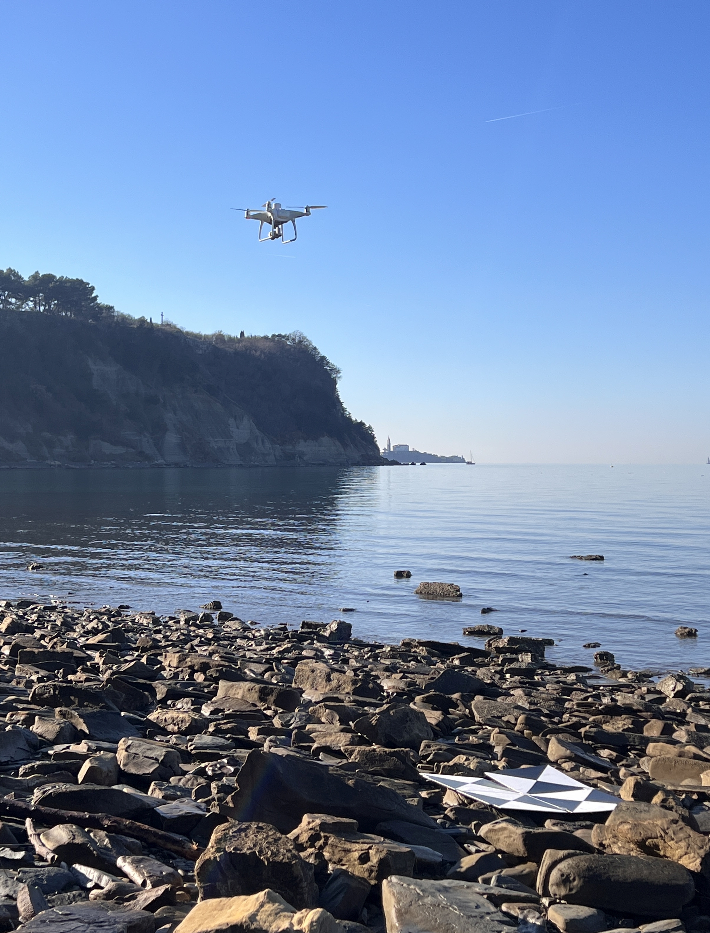
UAV surveys were performed with DJI Phantom 4 RTK. The goal was to fly as close as possible, but at a safe distance, to the cliff walls to capture morphologic details at high resolution. All UAV flights were automated with pre-planned missions. As the cliffs are steep, most of them are inclined around 100 % or 45°, a regular topographic survey with nadir images taken from the constant height from the take-off points is not an option. The height differences exceed 50 meters in some parts. Even capturing nadir images at a selected height above ground applying so-called terrain following mode is not optimal because some specific features could remain undetected. The optimal solutions would be taking images with their optical axis perpendicular to the cliff walls. Phantom 4 RTK features a flight mode which is well suited for such tasks. The 'Angled Flight Route' mode takes any plane, consisting of three points – these can be pre-entered via KML file or flown to before the mission – and flies at a selected distance from the plane. The image can be taken vertically or perpendicular to the plane. An example of creating a mission is shown in Figure 5a. A, B and C are the points which define the plane. The extents from point C, parallel to the line AB, are custom. The selected distance from the surface was 25 meters for most areas and 15 meters for 2 specific regions. The Ground Sampling Distance (GSD) at those distances is 0.68 and 0.41 cm, respectively.
The surveyed area was split into 11 sectors, each of them was captured by a predefined Angled Flight Route mission. Sectors 7 and 11 were observed at 15 meters, all the others at 25 meters from the imaginary plane. Figure 6 shows the sectors with their respective labels. Sector 5 is the one that was also observed with TLS.
The UAV flights were performed in the RTK GNSS. Because of the weak or non-existent data mobile network in some parts, it was impossible to use the Slovenian CORS (Continuously Operating Reference Station) network in real-time. Therefore, four base station points were stabilized and measured in the geodetic traverse along with GCPs. Three of them, labeled S2, S3 and S4 (see Figure 6), lying between the sea and the cliff walls, were used as RTK base stations utilizing DJI D-RTK 2. An example of the base station set on a point is shown in Figure 5b. Beside direct georeferencing of aerial images, the GCPs were also used in processing.
2.4. TLS and UAV surveys
Ten TLS and eight UAV surveys were carried out between April 2019 and April 2024. They are listed in Table 1. Seven consecutive and six cumulative pairs can be created for comparison.
It was not always possible to execute both UAV and TLS surveys simultaneously. Some of the epochs are 2 weeks within each other (labelled in green), some are further apart (red and yellow labels).
Table 2 lists consecutive and cumulative pairs, created from TLS and UAV epochs.
2.5. Methods of Comparison
2.5.1. Mesh Comparison (M3C2)
Surface changes can be represented graphically as (1) distances between point clouds or (2) distances between surface models such as M3C2 [15,16]. The latter method is far better as the former does not provide signed values. The standard linear color scale for visualizing changes uses red to indicate negative changes (erosion), blue for positive changes, and white for changes smaller than the accuracy threshold. In Figure 7, negative changes are clearly visible in the steep sections — rockfall events— while material accumulation can be observed on the scree slopes below the cliff.
2.5.2. Difference of DEM (DoD)
Since we want to evaluate the differences between the methods quantitatively and not just visually, we consider a DoD grid [17] to be the most appropriate way to represent these differences. Due to the presence of harder flysch layers - ledges that protrude from the cliff face - we need to choose a projection plane for the DEM that is roughly parallel to the cliff surface to avoid shadows in the surface model. This ensures that the height component is perpendicular to the average plane of the cliff wall, while the x-axis remains horizontal (Figure 8).
The next challenge is vegetation. Due to the fundamentally different data acquisition methods, interfering vegetation affects the data collected with each method differently. In order to properly evaluate the differences between methods, errors caused by unremoved vegetation cannot be ignored. The most effective way to mitigate these issues appears to be to analyze smaller vegetation-free patches that are distributed as evenly as possible over the entire cliff surface (Figure 9).
Ten clearly defined Regions of Interest (ROI) of different sizes were defined in a uniform coordinate system that is identical for all data collected with both methods. For each ROI, the captured point cloud was resampled into a raster with a density of 2 cm (which corresponds approximately to the point density in the field). This results in matrices with 2,500 cells per square meter, where the cell values represent terrain elevation (in metric units) in the direction perpendicular to the average plane of the cliff (Figure 9, Table 4).
The DoD for each pair of epochs and both data acquisition methods is simply calculated as the difference between the matrices representing the DEM of each ROI in each epoch. The DoD is easily represented graphically, see Figure 10, using the same standard color scale as M3C2: a linear gradient from red (decrease in terrain level) to white (no change) and to blue (increase in terrain level).
3. Results
3.1. UAV results
UAV survey data was processed in Agisoft Metashape software. The results of SfM/MVS processing are: dense point cloud, 3D model, DSM (Digital Surface Model), DTM (Digital Terrain Model) and orthophoto. For comparison of UAV surveys between different epochs or combining UAV and TLS data, point clouds, 3D models or DTMs can be used. Because sectors 1 and 2 (see Figure 5) are separated, they were processed individually. Sectors 3 to 10 were processed together to strengthen the solutions and provide better fit. During the observation period, some of the bolts for GCPs slipped due to rockfalls or were covered with scree. Missing GCPs might cause a weak solution for a single sector. Therefore, to mitigate the lack of GCPs in certain spots, all the adjoining sectors were processed together.
For the last UAV survey, on 21 March 2024, 2102 images of sectors 3-10 resulted in over 513 million points in the point cloud. The mesh of the 3D model has over 204 million faces. Both include only the cliffs, the forested areas above the cliffs have been removed. 3D model of the area is displayed in Figure 11.
3.2. UAV Surveys with Different Positioning Modes
UAV survey on 15 October 2021 was performed in two ways. One was RTK using DJI D-RTK 2 base station, a so-called direct georeferencing [18]. The other was none-RTK, using autonomous positioning. One of the GCPs, O22, was found to be destroyed. To perform quality control of different positioning modes, the remaining three GCPs and two points (T1, T2) near the top of the cliff were used. Locations of the points can be seen in Figure 14. The distance between O21 and O24 is 172 meters and the height difference between GCPs and test points T1 and T2 is 70 meters. Points T1 and T2 are distinctive features on the cliff and coordinates of T1 and T2 are measured on point clouds. Coordinates of GCPs are determined in the georeferencing part of processing.
According to our tests, the differences of RTK and PPK (Post-Processing Kinematic) coordinates are within 6 cm in each component. Similar values were determined by [18]. RTK and PPK solutions are treated as the same quality so only RTK and autonomous solutions are compared. Coordinate discrepancies between different solutions and given coordinates are stated in Table 5 and Table 6.
According to RTK results, there is no real use of GCPs as there is only a minor improvement. The accuracy at T1 and T2 is within the accuracy of the coordinate reading, which is around 5 cm.
The situation differs significantly for autonomous solutions, where GCPs play a crucial role. However, since GCPs can only be placed in the lower part of the cliff, the accuracy improvement is limited to that region. As a result, coordinate errors at T1 and T2 may still exceed 1 meter, rendering the solution unreliable for practical applications.
3.3. Comparison Between UAV and TLS Results
The sum of all positive cell values can be calculated for each DoD. Multiplied by the cell area, this gives the total volume increase corresponding to sedimentation — an unexpected phenomenon on a vertical cliff. Similarly, the addition of all negative cell values gives the total volume of erosion. An important statistical parameter for each DoD is the mean change value, which is calculated as the average of all cell values. Since the distribution of cell values is not standardized, histograms of cell value distributions provide valuable insights into the similarity of changes between two DoDs.
The differences in DoDs between the acquisition methods for a given ROI and epoch pair are simply calculated as the difference between the respective DoDs. These differences can be visualized using the same graphical approach. However, since they represent discrepancies between the change detection of the two methods, a different color scale is used. The mean value of the DoD differences corresponds to the difference between the mean cell values. The degree of similarity between the changes detected by TLS and UAV can also be quantified using the correlation coefficient between the vectorized DoD representations.
The results can be plotted for all or selected epoch pairs for each ROI. For ROI1 — the largest and potentially most representative — the results for selected epoch pairs are shown in Figure 15.
If the changes derived from the UAV were identical to those obtained from the TLS, the histograms (columns 2, 4 and 5) would consistently show similar shapes. A shift in the GCPs would likely cause a shift in the surface — at least within a small ROI. Similar histogram shapes indicate that comparable changes were detected, while a shift between the histograms indicates that the detected magnitudes are either over- or underestimated.
The "Diff of DoD" (column 6 in Figure 15) should ideally appear white and its histogram on the right should follow a standard normal distribution representing the sum of the random errors of both methods. A uniform color in the "Diff of DoD" visualization indicates a consistent offset across the entire ROI, likely due to georeferencing discrepancies. Conversely, localized patches in the "Diff of DoD" visualization indicate details that were only captured by one of the two compared methods.
Table 7 shows numerical values for the data from Figure 15. V+ stands for a positive change in volume (sedimentation), V- for a negative change in volume (erosion) and mean value for the average change in height over the entire area of ROI1. The correlation coefficient between the two DoDs and the average difference between them is also calculated.
4. Discussion
4.1. RTK and Autonomous Positioning of UAV Surveys
According to the results listed in Table 5 and Table 6 and due to the severe limitations in setting GCPs, direct georeferencing, whether RTK or PPK, is the only option. With autonomous solutions, the position error can easily exceed 1 meter at a distance of more than 50 meters from GCPs.
In the case of direct georeferencing, the results (Table 5 upper part) show that no GCPs are required. However, some of our other cases prove the opposite. Especially the height component is vulnerable. The use of GCPs is highly advisable, as also mentioned in [18]. The geometric distribution should be similar over the whole observed area. As already mentioned, this task is impossible to fulfill in steep cliff walls. Therefore, the GCPs should be placed at least in the accessible lower parts of the cliffs.
4.2. UAV Surveys
UAV surveys can be carried out in nadir or oblique manner. Nadir imagery may miss some topographic features in steep terrain. In addition, there are large differences in scales of captured images. Therefore, oblique imaging is preferred for steep rock faces. To capture the terrain at a similar GSD, the drone should fly at a similar distance from the wall. The drone used was able to fly and capture image perpendicular to the target surface.
After SfM/MVS processing, UAV photogrammetry delivers various products that are suitable for comparisons, analyzes and visualizations. Point clouds, meshes or DTMs can be used for terrain comparisons, whether at different epochs using the same technique or in conjunction with TLS. With the results of periodic UAV surveys, rockfalls can be easily identified.
4.3. Comparison Between UAV and TLS Results
The results only for the largest and most representative area ROI1 are presented in Figure 15 and Table 7. Epoch pairs were selected where the TLS and UAV measurements were close in time. The pair of epochs to be compared is indicated on the left-hand side of Figure 15.
The first column shows the detected changes (DoD) for TLS technology, the third column shows the same for UAV. The second and fourth columns contain the histograms of the DoD changes. In the TLS histograms, we find that most of the changes are negative, which is to be expected for a steep cliff where large amounts of material cannot accumulate. However, in ROI1 there is a section of scree below the cliff where material can accumulate. The average values of the histograms increase with the increasing time interval between the epochs (see also Table 7, column "TLS mean").
The fourth column shows the DoD histograms for the UAV method. The first row (3-5) is very similar to the TLS data. In the second row (5-6), however, there is a clear discrepancy, with UAV showing a change of 4.3 cm (see Table 7, column "Mean diff."), which is quite surprising and probably due to a shift in the GCPs. For epoch pairs 6-8 and 8-10, the changes are again almost identical to TLS (see Table 7). In the last three rows (3-6, 3-8 and 3-0), a consistent offset of 6-7 cm is observed. These three discrepancies are probably due to a shift in GCPs between epochs 5 and 6, which is reflected in all epoch pairs where the first epoch is smaller than 5 and the second epoch is larger than 6.
The standard deviations of the differences between the UAV and TLS DoDs (columns 6 and 7 in Figure 15) are consistently around 5 cm, which indicates the sum of the accuracies of both measurement methods. So even if there is an absolute difference (probably due to georeferencing), the dispersion of the differences remains constant, which means that both methods captured the same surface shape. This suggests that there are no internal distortions or errors, which is promising for the use of UAVs. However, greater caution is required with GCPs.
Looking specifically at the three consistent epoch pairs (3-5, 6-8, 8-10), the average differences are only 14, -4 and 14 mm respectively, with dispersions of 60, 41 and 49 mm. For the pairs with offsets (5-6, 3-6, 3-8, 3-10), the average differences are 49, 63, 59 and 73 mm respectively, indicating that a shift has probably occurred between epochs 3 and 5 (14 mm). Otherwise, the offset is consistent. There is no clear trend in the dispersion of the differences. The most plausible explanation is that the dispersion is simply the sum of the random errors of both acquisition methods.
5. Conclusions
Detecting changes in steep terrain, such as cliffs, is a challenging endeavor. First of all, ground targets must be set. We have established a closed geodetic traverse with a combination of GNSS and TPS surveying to ensure the highest possible accuracy and quality control. The UAV must be carried out in direct georeferencing mode (RTK or PPK). For steep rock faces, the use of a special flight mode that follows the terrain and captures oblique images is very advantageous compared to normal flight at constant altitude and nadir imaging.
The TLS survey of cliffs is even more demanding. The flat area at the foot of the cliffs is usually too narrow to obtain a proper viewpoint for the TLS. Bays and straits have better potential for cliff TLS surveys. But in such cases, the range of the TLS is a limiting factor. Also, accuracy and resolution decrease with distance. We surveyed part of the cliffs with UAV and TLS. To mitigate other interfering factors, such as vegetation, the area was divided into different ROIs. To keep the article within a manageable scope, only one ROI is presented with results. The comparison, see 4.3., shows some small discrepancies between the two surveying methods, but generally leads to similar trends. Considering the limitations of setting up TLS and UAV open space with the option to fly close to the cliff faces, it can be concluded that UAV is more suitable for cliff surveying.
In any case, several restrictions must be considered when surveying. Accessibility is usually the most limiting factor. When surveying by UAV, rain, wind and tides must be taken into account. Some parts of our case study can only be reached at low tide. Vegetation is another issue. For this reason, we conduct the surveys in early spring and late fall or early winter when the foliage is at its lowest. Not to forget, the cliffs, unlike most other rocks, are active. There is constant erosion caused by rain, seawater and wind. The erosion sometimes leads to a rockfall. Even if a GCP is set to the highest accuracy, the actual location can shift due to erosion or be destroyed by a rockfall.
In the future, we will continue the surveys to determine the average rate of erosion-induced changes. During the upcoming surveys we will try different capturing methods, different instruments and additional processing of the acquired data. Laser scanning with a UAV is also on the list of future options.
Author Contributions
Conceptualization, K.K. and K.K.T.; methodology, K.K. and K.K.T.; validation, K.K. and K.K.T.; formal analysis, K.K. and K.K.T.; investigation, K.K. and K.K.T.; resources, K.K. and K.K.T.; data curation, K.K. and K.K.T.; writing—original draft preparation, K.K. and K.K.T.; writing—review and editing, K.K. and K.K.T.; visualization, K.K. and K.K.T. All authors have read and agreed to the published version of the manuscript.
Funding
The authors acknowledge the financial support from the Slovenian Research and Innovation Agency (research core funding No. P2-0227 Geoinformation infrastructure and sustainable spatial development of Slovenia) and research project J1-2477 Erosional processes on coastal flysch cliffs and their risk assessment.
Conflicts of Interest
The authors declare no conflict of interest. The funders had no role in the design of the study; in the collection, analyses, or interpretation of data; in the writing of the manuscript, or in the decision to publish the results.
Abbreviations
The following abbreviations are used in this manuscript:
| GNSS | Global Navigation Satellite Systems |
| RTK | Real Time Kinematic |
| PPK | Post-Processing Kinematic |
| CORS | Continuously Operating Reference Station |
| UAV | Unmanned Aerial Vehicle |
| TLS | Terrestrial Laser Scanning |
| TPS | Total Positioning Station |
| GCP | Ground Control Point |
| SfM | Structure from Motion |
| MVS | Multi-View Stereo |
| GSD | Ground Sampling Distance |
| DEM | Digital Elevation Model |
| DSM | Digital Surface Model |
| DTM | Digital Terrain Model |
| DoD | Difference of DEM |
| ROI | Region of interest |
References
- Cirillo, D.; Zappa, M.; Tangari, A.C.; Brozzetti, F.; Ietto, F. Rockfall Analysis from UAV-Based Photogrammetry and 3D Models of a Cliff Area. Drones 2024, 8, 31. [Google Scholar] [CrossRef]
- Barlow, J.; Gilham, J.; Ibarra Cofrã, I. Kinematic Analysis of Sea Cliff Stability Using UAV Photogrammetry. International Journal of Remote Sensing 2017, 38, 2464–2479. [Google Scholar] [CrossRef]
- Rosser, N.J.; Petley, D.N.; Lim, M.; Dunning, S.A.; Allison, R.J. Terrestrial Laser Scanning for Monitoring the Process of Hard Rock Coastal Cliff Erosion. QJEGH 2005, 38, 363–375. [Google Scholar] [CrossRef]
- Tyszkowski, S.; Zbucki, Ł.; Kaczmarek, H.; Duszyński, F.; Strzelecki, M.C. Terrestrial Laser Scanning for the Detection of Coastal Changes along Rauk Coasts of Gotland, Baltic Sea. Remote Sensing 2023, 15, 1667. [Google Scholar] [CrossRef]
- Hoffmeister, D.; Tilly, N.; Curdt, C.; Aasen, H.; Ntageretzis, K.; Hadler, H.; Willershäuser, T.; Vött, A.; Bareth, G. Terrestrial Laser Scanning for Coastal Geomorphologic Research in Western Greece. Int. Arch. Photogramm. Remote Sens. Spatial Inf. Sci. 2012, XXXIX-B5, 511–516. [Google Scholar] [CrossRef]
- Kersten, T.P.; Lindstaedt, M.; Mechelke, K. Coastal Cliff Monitoring Using UAS Photogrammetry and TLS. HN 2020, 16–22. [Google Scholar] [CrossRef]
- Kuhn, D.; Prüfer, S. Coastal Cliff Monitoring and Analysis of Mass Wasting Processes with the Application of Terrestrial Laser Scanning: A Case Study of Rügen, Germany. Geomorphology 2014, 213, 153–165. [Google Scholar] [CrossRef]
- Rosser, N.J.; Brain, M.J.; Petley, D.N.; Lim, M.; Norman, E.C. Coastline Retreat via Progressive Failure of Rocky Coastal Cliffs. Geology 2013, 41, 939–942. [Google Scholar] [CrossRef]
- Doran, T.A.; Kennedy, D.M.; McCarroll, J.R.; Allan, B.M.; Ierodiaconou, D. Using UAV-Derived Point Clouds to Measure High Resolution Cliff Dynamics in Soft Lithologies: Demons Bluff, Victoria, Australia 2024.
- Son, S.W.; Kim, D.W.; Sung, W.G.; Yu, J.J. Integrating UAV and TLS Approaches for Environmental Management: A Case Study of a Waste Stockpile Area. Remote Sensing 2020, 12, 1615. [Google Scholar] [CrossRef]
- Minervino Amodio, A.; Di Paola, G.; Rosskopf, C.M. Monitoring Coastal Vulnerability by Using DEMs Based on UAV Spatial Data. IJGI 2022, 11, 155. [Google Scholar] [CrossRef]
- Jaud, M.; Letortu, P.; Théry, C.; Grandjean, P.; Costa, S.; Maquaire, O.; Davidson, R.; Le Dantec, N. UAV Survey of a Coastal Cliff Face – Selection of the Best Imaging Angle. Measurement 2019, 139, 10–20. [Google Scholar] [CrossRef]
- Konsolaki, A.; Karantanellis, E.; Vassilakis, E.; Kotsi, E.; Lekkas, E. Multitemporal Monitoring for Cliff Failure Potential Using Close-Range Remote Sensing Techniques at Navagio Beach, Greece. Remote Sensing 2024, 16, 4610. [Google Scholar] [CrossRef]
- Riegl VZ-400 2017.
- James, M.R.; Robson, S.; Smith, M.W. 3-D Uncertainty-based Topographic Change Detection with Structure-from-motion Photogrammetry: Precision Maps for Ground Control and Directly Georeferenced Surveys. Earth Surf Processes Landf 2017, 42, 1769–1788. [Google Scholar] [CrossRef]
- Lague, D.; Brodu, N.; Leroux, J. Accurate 3D Comparison of Complex Topography with Terrestrial Laser Scanner: Application to the Rangitikei Canyon (N-Z). ISPRS Journal of Photogrammetry and Remote Sensing 2013, 82, 10–26. [Google Scholar] [CrossRef]
- Wheaton, J.M.; Brasington, J.; Darby, S.E.; Sear, D.A. Accounting for Uncertainty in DEMs from Repeat Topographic Surveys: Improved Sediment Budgets. Earth Surf Processes Landf 2010, 35, 136–156. [Google Scholar] [CrossRef]
- Liu, X.; Lian, X.; Yang, W.; Wang, F.; Han, Y.; Zhang, Y. Accuracy Assessment of a UAV Direct Georeferencing Method and Impact of the Configuration of Ground Control Points. Drones 2022, 6, 30. [Google Scholar] [CrossRef]
- Šinkovec, Anja Positioning quality analysis of an unmanned aerial vehicle with direct georeferencing: the use of RTK and PPK method. Master Thesis, University of Ljubljana: Ljubljana, 2021.
Figure 1.
The location of the cliff case study area near Strunjan, shown on a national orthophoto.
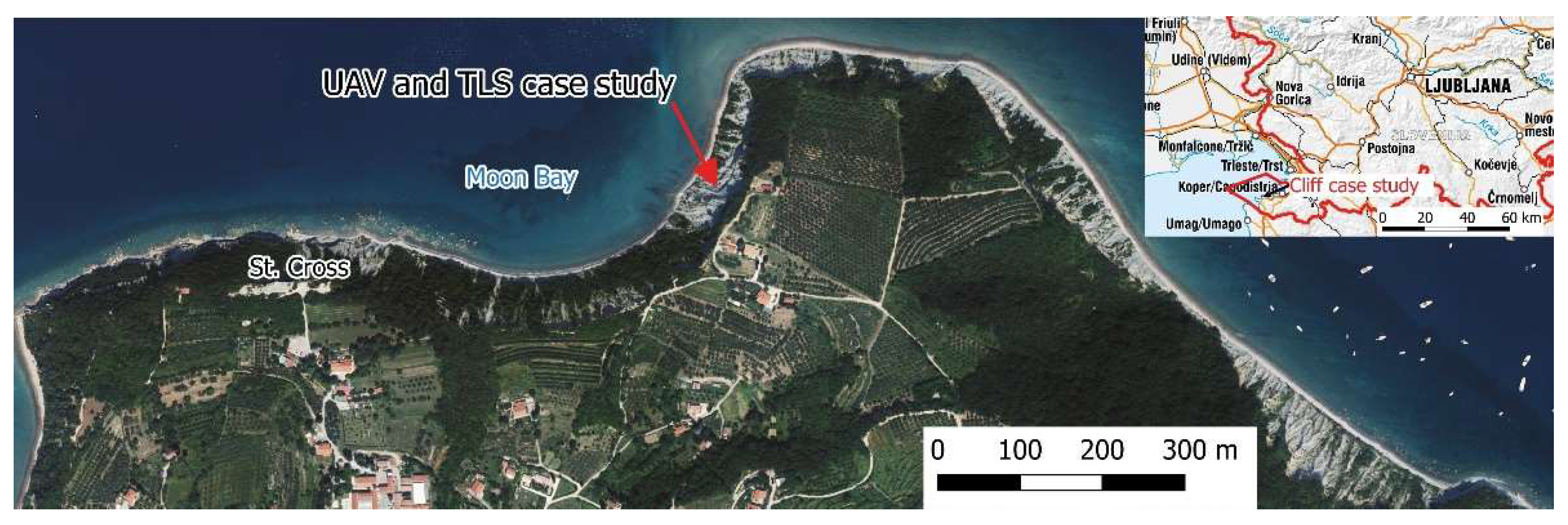
Figure 2.
The locations of GCPs for TLS (left) and UAV (right).
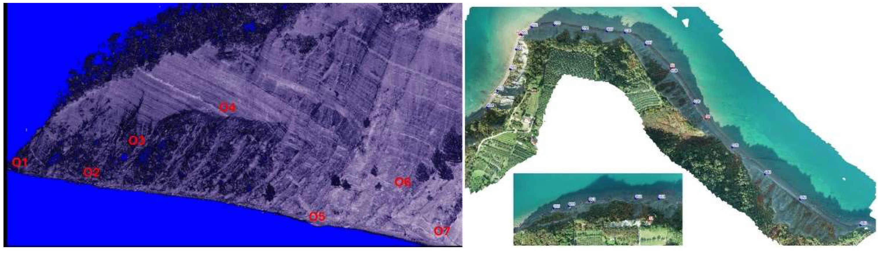
Figure 3.
Geodetic network of GCPs connected to GNSS points with standard error ellipses.
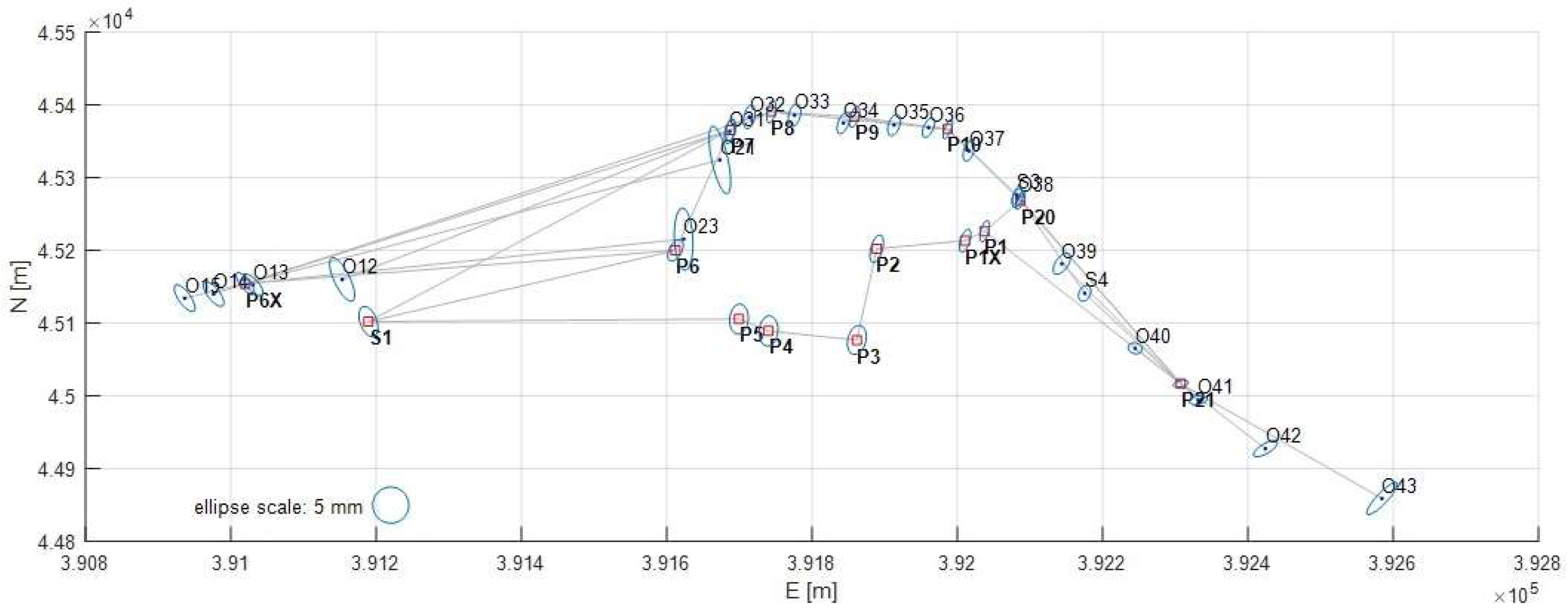
Figure 4.
TLS setup overviewing the selected section of the cliff.
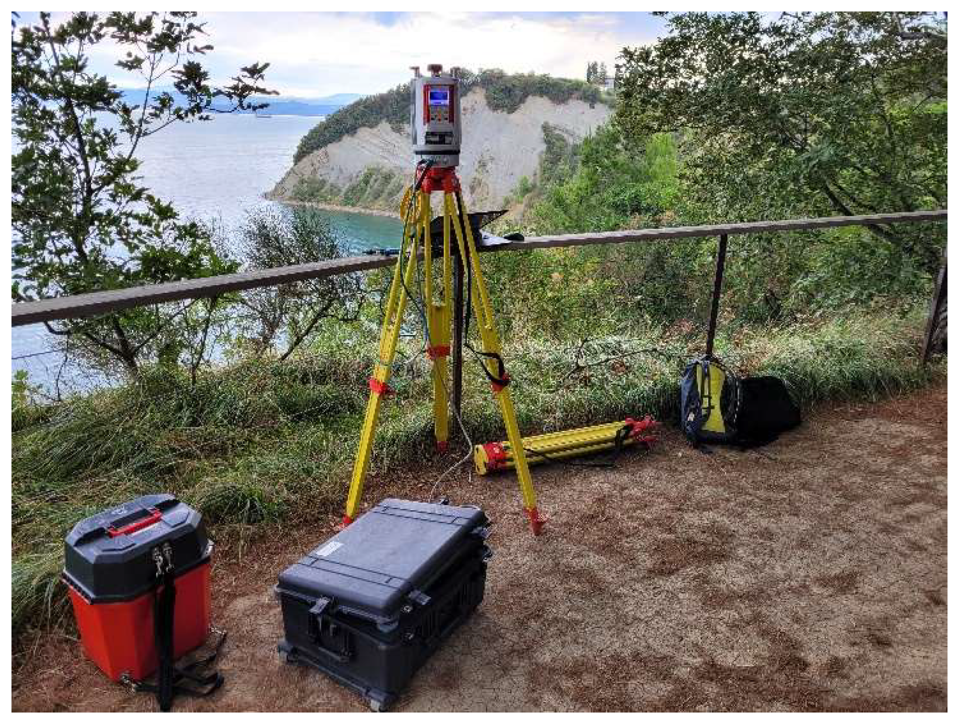
Figure 5.
a) Screenshot of the DJI Fly application with the Angled Flight Route mission; b) RTK-UAV base station, UAV and a provisional landing pad.
Figure 5.
a) Screenshot of the DJI Fly application with the Angled Flight Route mission; b) RTK-UAV base station, UAV and a provisional landing pad.
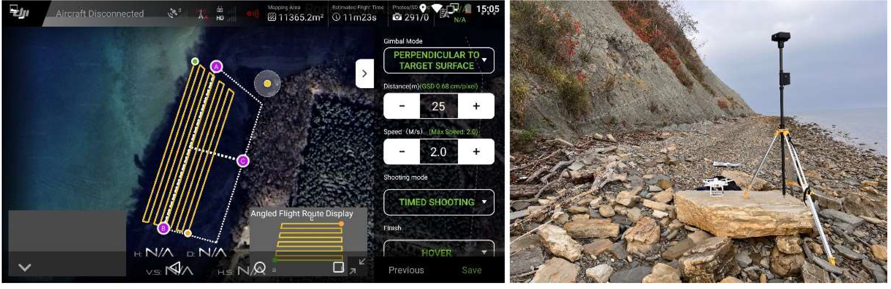
Figure 6.
Locations of UAV GCPs (blue labels), RTK base stations (red labels) and surveyed sectors (transparent polygons, black labels), shown on the UAV derived orthophoto.
Figure 6.
Locations of UAV GCPs (blue labels), RTK base stations (red labels) and surveyed sectors (transparent polygons, black labels), shown on the UAV derived orthophoto.
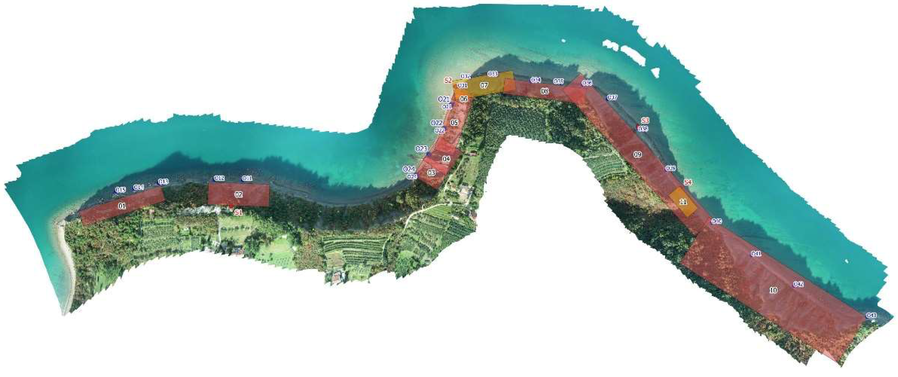
Figure 7.
Example for the visualization of a mesh2mesh comparison.
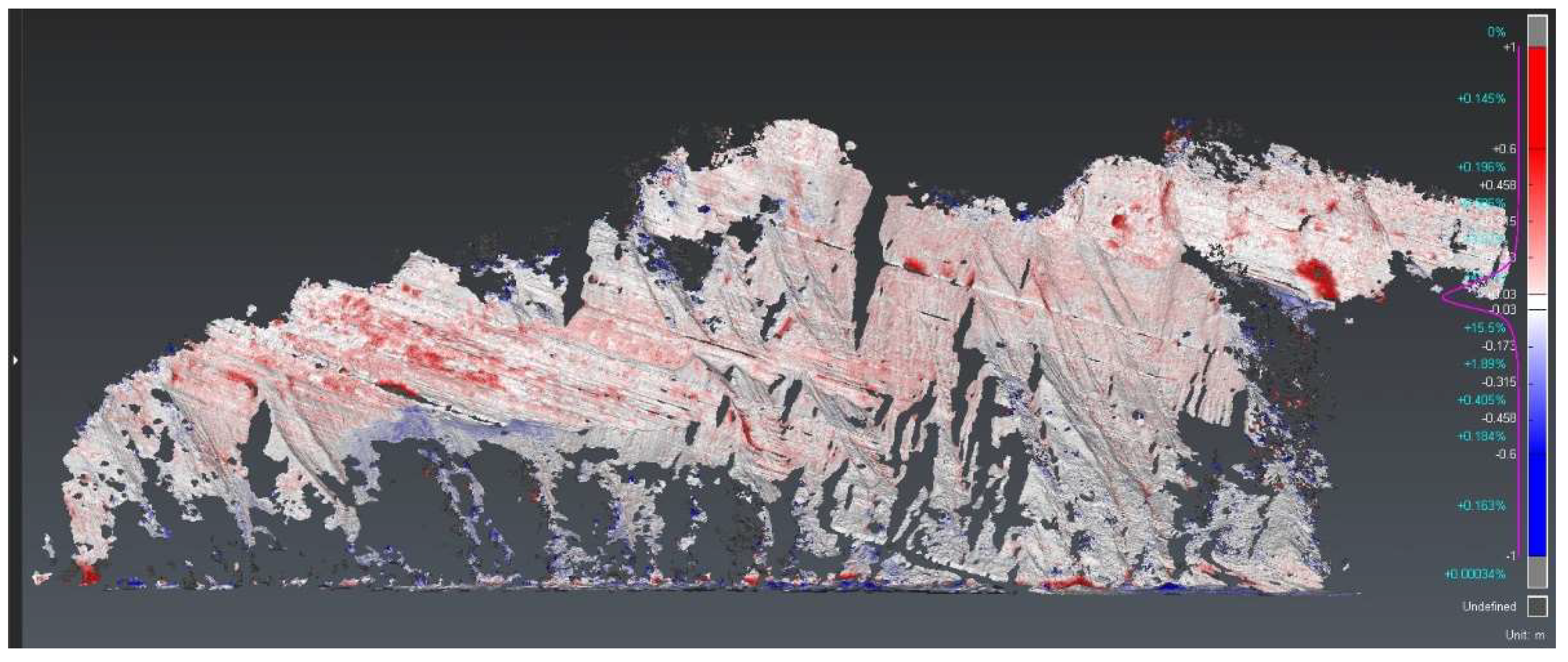
Figure 8.
Transformation of the point cloud into the coordinate system of the cliff wall.
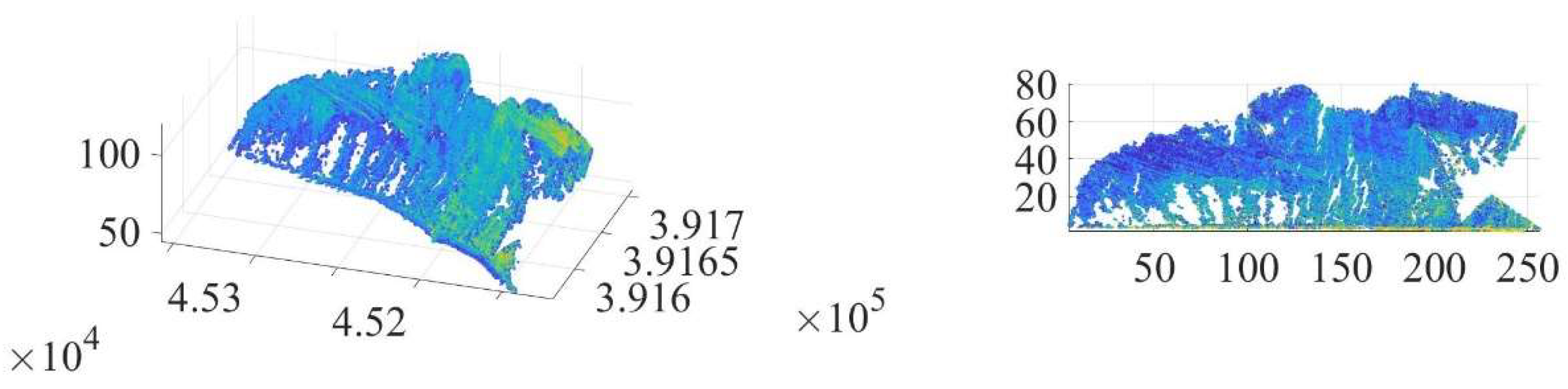
Figure 9.
Regions of interest on TLS and UAV point clouds.
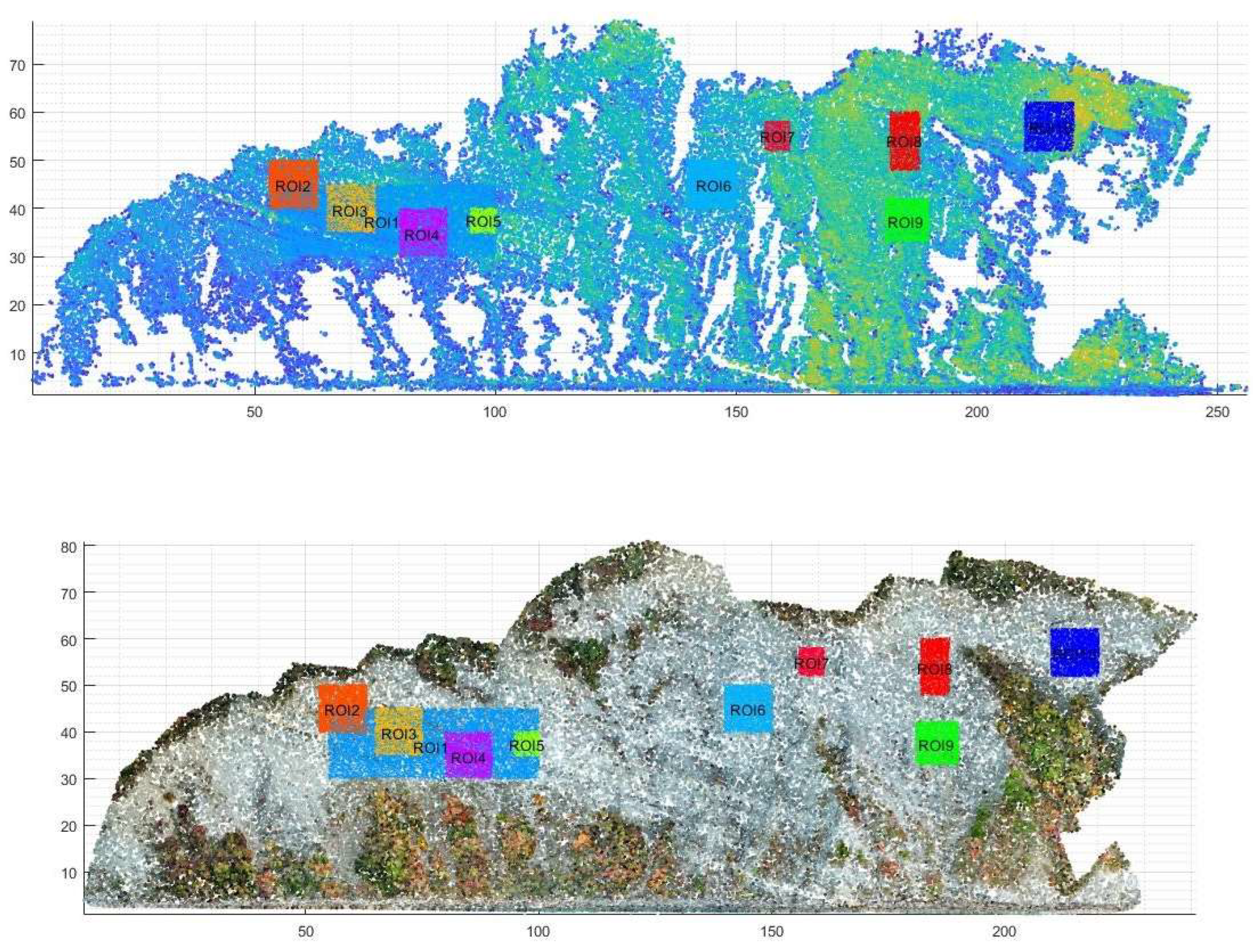
Figure 10.
Example for the visualization of a DoD comparison.
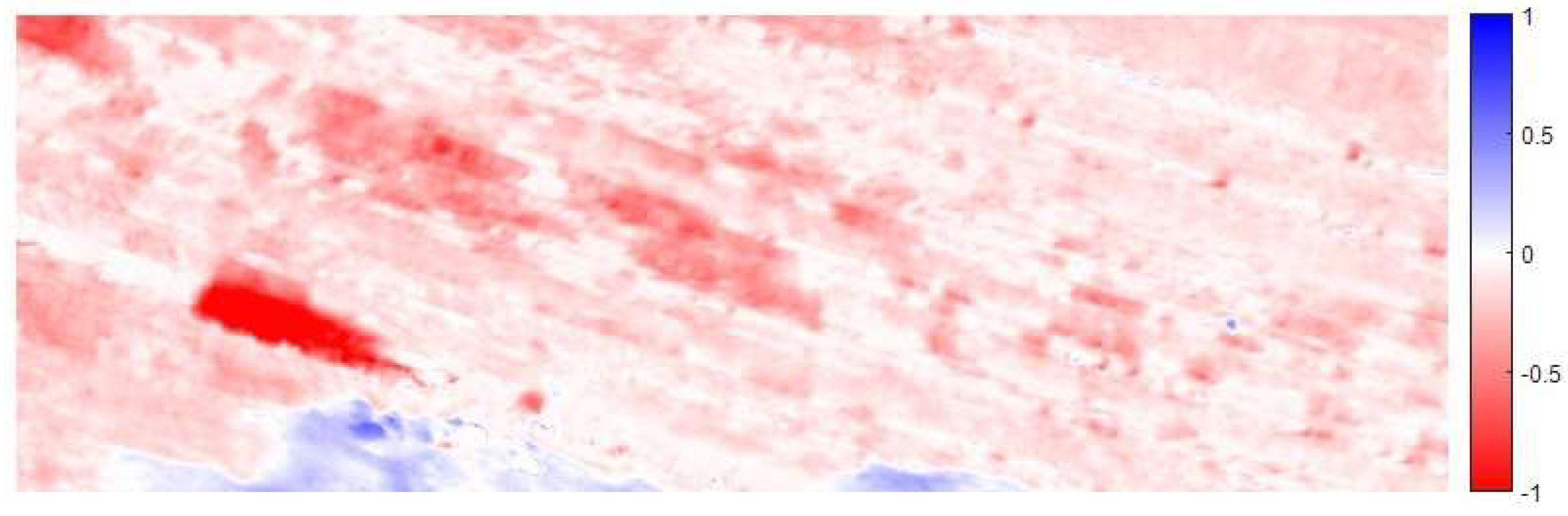
Figure 11.
3D model of the cliffs and the remaining GCPs.
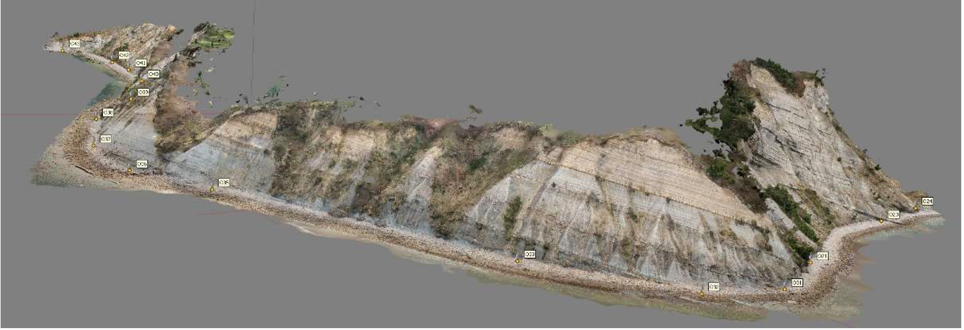
Figure 12.
Selected areas of rockfalls.
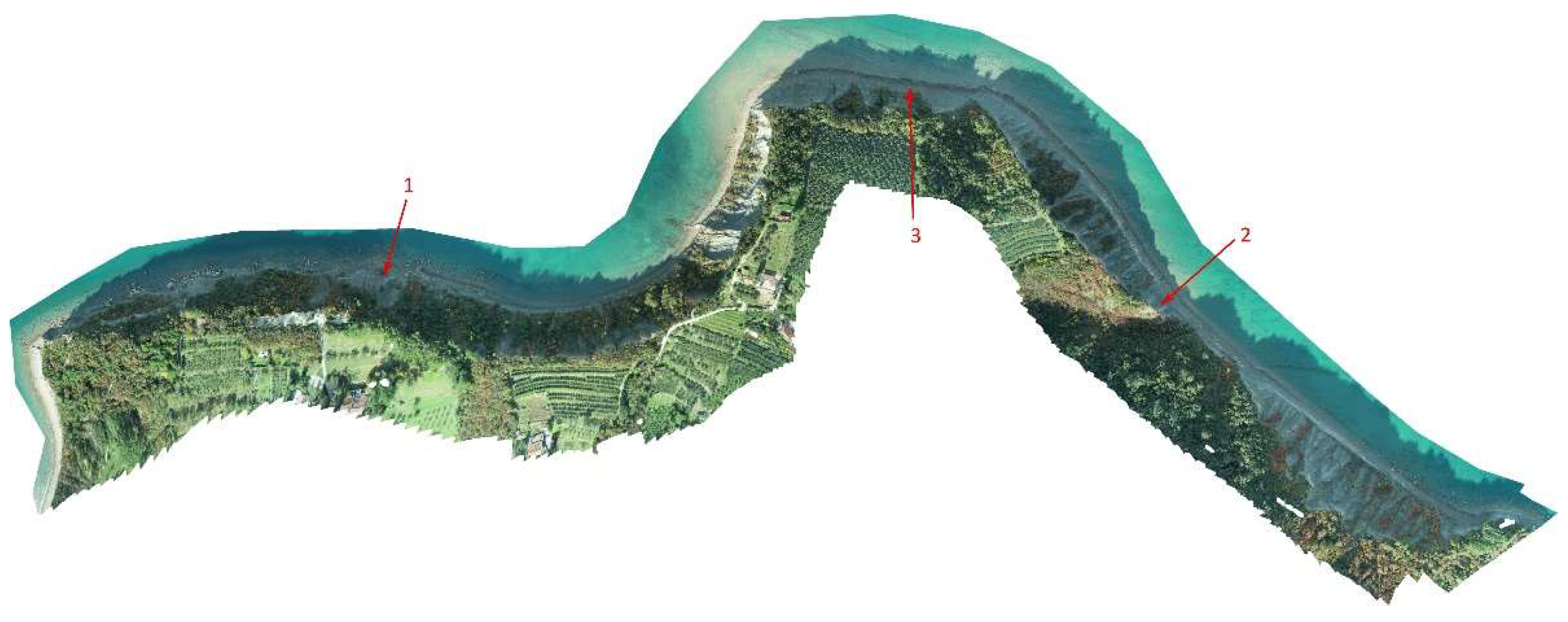
Figure 13.
DoDs of rockfall cases, calculated in Global Mapper Pro. The accumulations of the fallen material (shades of green and blue) are shown in shades of orange and red.
Figure 13.
DoDs of rockfall cases, calculated in Global Mapper Pro. The accumulations of the fallen material (shades of green and blue) are shown in shades of orange and red.
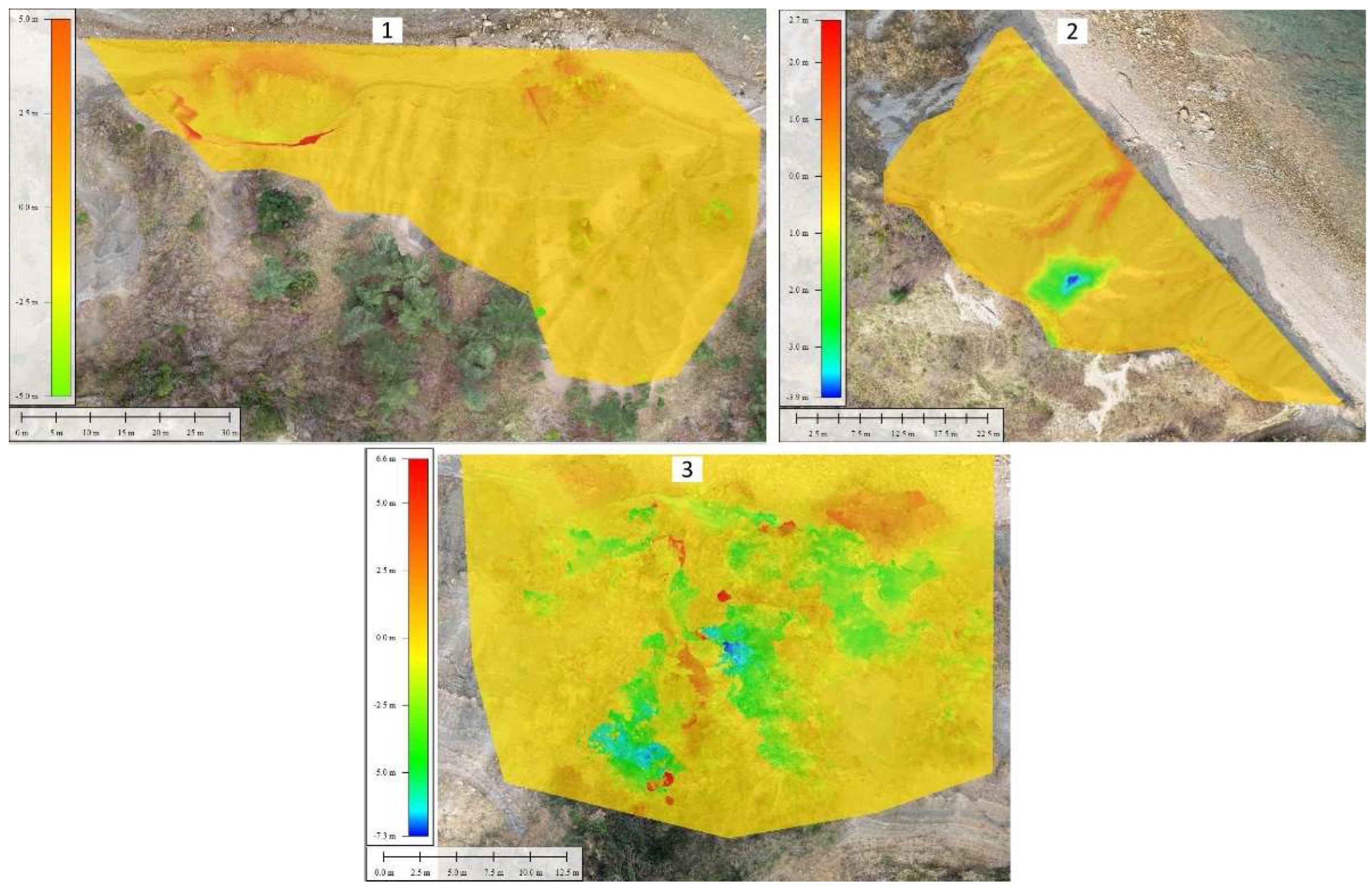
Figure 14.
GCPs and check points.
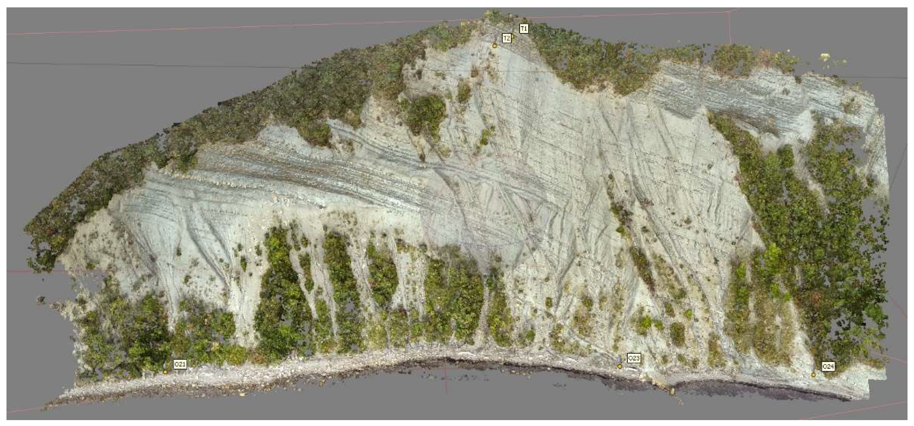
Figure 15.
Comparison of results between UAV and TLS for ROI1 (column 1: DoD for TLS; column 2: histogram of DOD values for TLS; column 3: DoD for UAV; column 4: histogram of DoD values for UAV; column 5: both histograms in the same image; column 6: difference between both DoDs; column 7: histogram of column 6).
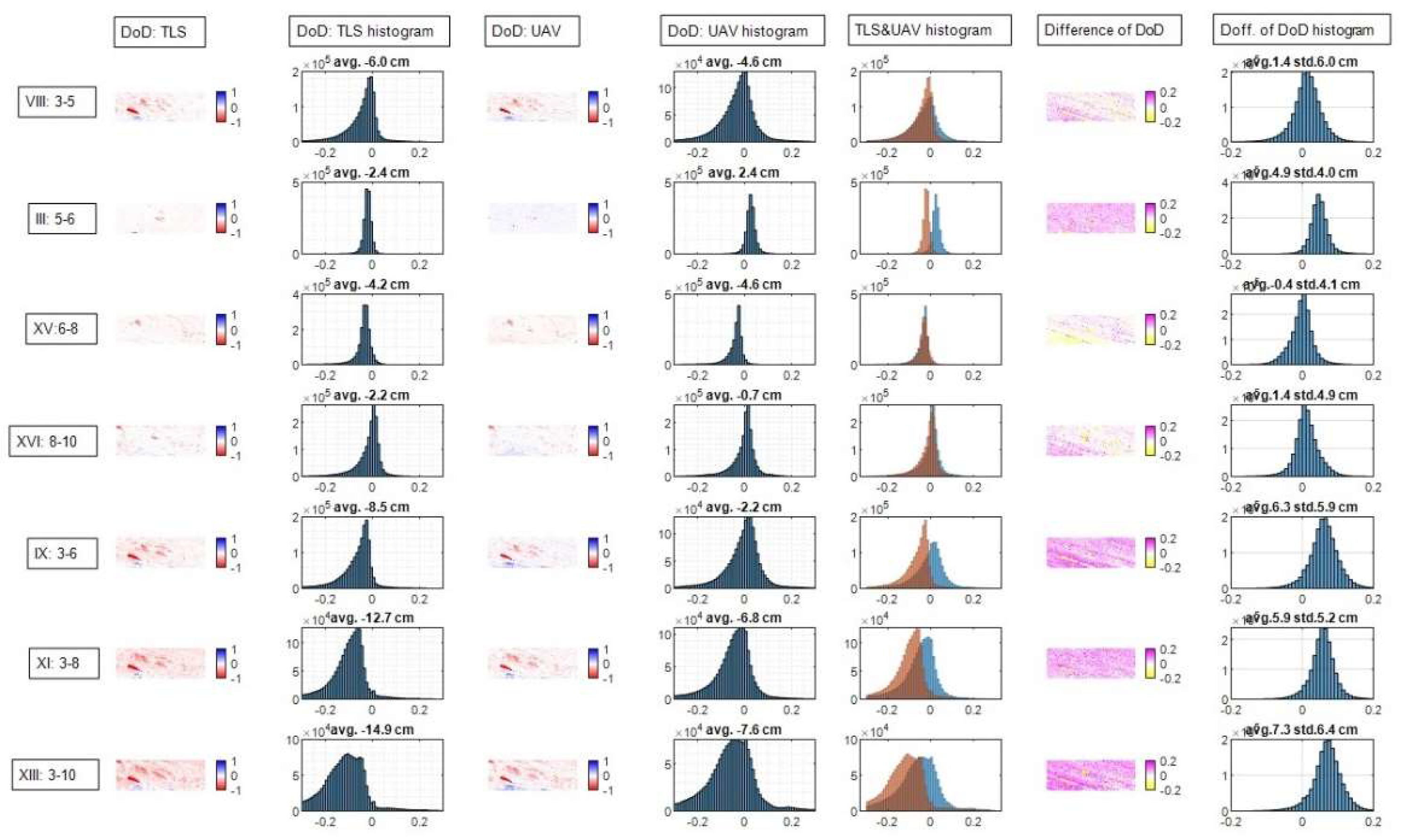

Table 1.
TLS and UAV survey epochs.
| TLS epochs | UAV epochs | TPS CP campaign | |
|---|---|---|---|
| 1 | 17 April 2019 | ||
| 2 | 28 January 2020 | ||
| 3 | 9 November 2020 | 9 November 2020 | 28 October 2020 |
| 4 | 14 April 2021 | 26 March 2021 | |
| 5 | 13 October 2021 | 15 October 2021 | |
| 6 | 28 March 2022 | 22 March 2022 | |
| 7 | 29 October 2022 | 7 December 2022 | |
| 8 | 10 April 2023 | 7 April 2023 | |
| 9 | 16 January 2024 | 12 September 2023 | |
| 10 | 5 April 2024 | 21 March 2024 | 5 April 2024 |
Table 2.
Consecutive and cumulative pairs.
| Epoch pair | consecutive | Epoch pair | cumulative | ||||
|---|---|---|---|---|---|---|---|
| I | 3 | 4 | nov 2020 & apr 2021 | ||||
| II | 4 | 5 | apr 2021 & oct 2021 | VIII | 3 | 5 | nov 2020 & oct 2021 |
| III | 5 | 6 | oct 2021 & mar 2022 | IX | 3 | 6 | nov 2020 & mar 2022 |
| IV | 6 | 7 | mar 2022 & nov 2022 | X | 3 | 7 | nov 2020 & nov 2022 |
| V | 7 | 8 | nov 2022 & apr 2023 | XI | 3 | 8 | nov 2020 & apr 2023 |
| VI | 8 | 9 | apr 2023 & jan 2024 | XII | 3 | 9 | nov 2020 & jan 2024 |
| VII | 9 | 10 | jan 2024 & apr 2024 | XIII | 3 | 10 | nov 2020 & apr 2024 |
Table 3.
Additional pairs.
| Epoch pair | selected | ||
|---|---|---|---|
| XV | 6 | 8 | mar 22 – apr 23 |
| XVI | 8 | 10 | apr 23 – apr 24 |
Table 4.
Dimensions and areas of ROIs.
| ROI | Dim [m] | Area [m2] |
|---|---|---|
| ROI1 | 45x15 | 675 |
| ROI2 | 10x10 | 100 |
| ROI3 | 10x10 | 100 |
| ROI4 | 10x10 | 100 |
| ROI5 | 5x5 | 25 |
| ROI6 | 10x10 | 100 |
| ROI7 | 5x6 | 30 |
| ROI8 | 6x12 | 72 |
| ROI9 | 9x9 | 81 |
| ROI10 | 10x10 | 100 |
| ROI1 | 45x15 | 675 |
Table 5.
Coordinate discrepancies of RTK solutions.
| solution | point | ΔE (m) | ΔN (m) | Δh (m) |
|---|---|---|---|---|
| RTK – no GCP | O21 | 0,08 | -0,04 | 0,01 |
| O23 | 0,05 | 0,00 | 0,00 | |
| O24 | 0,03 | -0,01 | 0,02 | |
| T1 | -0,04 | 0,05 | -0,03 | |
| T2 | 0,01 | -0,02 | 0,01 | |
| RTK + O23 | O21 | 0,07 | -0,04 | 0,01 |
| O23 | 0,04 | 0,00 | 0,00 | |
| O24 | 0,03 | -0,01 | 0,02 | |
| T1 | 0,02 | 0,03 | 0,04 | |
| T2 | -0,01 | -0,05 | 0,00 | |
| RTK + O21, O24 | O21 | 0,06 | -0,04 | 0,01 |
| O23 | 0,04 | 0,00 | 0,00 | |
| O24 | 0,02 | -0,01 | 0,02 | |
| T1 | 0,02 | 0,04 | 0,03 | |
| T2 | 0,01 | -0,04 | -0,03 | |
| RTK + O21, O23, O24 | O21 | 0,06 | -0,04 | 0,01 |
| O23 | 0,04 | 0,00 | 0,00 | |
| O24 | 0,02 | -0,01 | 0,02 | |
| T1 | 0,02 | 0,05 | 0,07 | |
| T2 | 0,00 | -0,01 | 0,01 |
Table 6.
Coordinate discrepancies of autonomous solutions.
| solution | point | ΔE (m) | ΔN (m) | Δh (m) |
|---|---|---|---|---|
| auton. – no GCP | O21 | -1,74 | 0,76 | 0,99 |
| O23 | -1,72 | 1,30 | 1,61 | |
| O24 | -1,48 | 1,81 | 1,72 | |
| T1 | -0,96 | 0,48 | 0,03 | |
| T2 | -1,01 | 0,39 | 0,00 | |
| auton. + O23 | O21 | -0,10 | 1,12 | 0,18 |
| O23 | 0,00 | 0,00 | 0,01 | |
| O24 | 0,14 | -0,21 | -0,35 | |
| T1 | -0,07 | -0,14 | 0,91 | |
| T2 | 0,01 | -0,17 | 0,89 | |
| auton. + O21, O24 | O21 | 0,00 | 0,01 | 0,01 |
| O23 | -0,10 | -0,20 | 0,24 | |
| O24 | 0,00 | 0,00 | 0,01 | |
| T1 | -0,78 | -0,22 | 1,04 | |
| T2 | -0,74 | -0,32 | 1,07 | |
| auton. + O21, O23, O24 | O21 | 0,01 | 0,05 | -0,02 |
| O23 | -0,07 | -0,13 | 0,10 | |
| O24 | 0,05 | 0,09 | -0,06 | |
| T1 | 0,17 | -0,71 | -0,15 | |
| T2 | 0,18 | -0,77 | -0,15 |
Table 7.
Numerical values of comparison of DoD from UAV and TLS capture of cliff surface.
| TLS | UAV | ||||||||
| ROI1 | Ep pair | V+ [m3] | V- [m3] |
mean [cm] | V+ [m3] | V- [m3] |
mean [cm] | Corr. coef. | Mean diff. [cm] |
| VIII: 3-5 | 4.73 | -45.5 | -6.03 | 10.81 | -42.01 | -4.61 | 0.911 | 1.4 | |
| III: 5-6 | 0.97 | -17.5 | -2.44 | 18.86 | -2.56 | 2.41 | 0.431 | 4.9 | |
| XV:6-8 | 0.82 | -29.28 | -4.21 | 0.65 | -31.88 | -4.62 | 0.711 | -0.4 | |
| XVI: 8-10 | 6.52 | -21.31 | -2.19 | 11.33 | -16.37 | -0.74 | 0.761 | 1.4 | |
| IX: 3-6 | 2.98 | -60.28 | -8.47 | 17.35 | -32.25 | -2.2 | 0.914 | 6.3 | |
| XI: 3-8 | 2.63 | -88.39 | -12.68 | 7 | -53.13 | -6.82 | 0.938 | 5.9 | |
| XIII: 3-10 | 3.75 | -104.29 | -14.87 | 11.62 | -62.79 | -7.57 | 0.921 | 7.3 | |
Disclaimer/Publisher’s Note: The statements, opinions and data contained in all publications are solely those of the individual author(s) and contributor(s) and not of MDPI and/or the editor(s). MDPI and/or the editor(s) disclaim responsibility for any injury to people or property resulting from any ideas, methods, instructions or products referred to in the content. |
© 2025 by the authors. Licensee MDPI, Basel, Switzerland. This article is an open access article distributed under the terms and conditions of the Creative Commons Attribution (CC BY) license (http://creativecommons.org/licenses/by/4.0/).
Copyright: This open access article is published under a Creative Commons CC BY 4.0 license, which permit the free download, distribution, and reuse, provided that the author and preprint are cited in any reuse.


