Submitted:
18 February 2025
Posted:
19 February 2025
You are already at the latest version
Abstract
Assessing risk in life cycle cost and benefit estimates of highway investments is recommended by major organizations such as the World Bank and the U.S. Federal Highway Administration. This challenging task needs methodological support. Mutually exclusive investment alternatives can differ in terms of costs of construction, maintenance, rehabilitation, and end of life value. Due to many causal factors and the long life of highway infrastructure, these items cannot be estimated with certainty. To go beyond sources of uncertainty study, a method is needed to check economic feasibility of acquiring additional information for deeper insight. This paper reports research on the value of Bayesian pre-posterior information for refining life cycle analysis of uncertain costs and benefits for evaluating highway investment alternatives. Example applications demonstrate how the Bayesian pre-posterior analysis can be applied to check the feasibility of obtaining new information for enhancing life cycle analysis of highway investments. The value of Bayesian pre-posterior information is illustrated for reducing risk. Also, depending upon specifics of uncertain states, a change in the choice of the investment alternative for implementation can be investigated. The product of this research can potentially upgrade highway infrastructure planning and management practice.
Keywords:
highway investments
; lifecycle analysis
; risk analysis
; Bayesian decision theory
; pre-posterior information
; value of information
; socio-economic impact
1. Introduction
Many well-known funding, research, and infrastructure sustainability agencies are promoting life cycle analysis as a basis for highway infrastructure investment decision-making. Also, they are recommending the study of risk in estimates of life cycle costs and benefits. Examples are the World Bank Institute [1], Federal Highway Administration (FHWA) [2,3], Transportation Research Board (TRB) [4] , and the Infrastructure Sustainability Institute (ISI) [5]. The importance of life cycle analysis and treating risk in investment decisions can be inferred from observations on sources of uncertainty in life cycle analysis and economic impacts of using uncertain estimates (Table 1). Further information on sources of uncertainty is provided below.
Given that mainly public funds are invested in highway infrastructure and uncertain socio-economic and socio-technical factors can compromise well-intended decisions, the importance of treating risk in life cycle estimates of costs and benefits is acknowledged by public agencies. For public-private partnership (PPS) infrastructure, this policy is also followed for reasons noted above [2,3,4,5,6].
The initial construction cost of a highway accounts for the highest component of life cycle cost due to many expensive items (i.e., land, materials, labor, etc.). But the importance of other items cannot be overlooked. Given the long life of the infrastructure (30 or more years), following the initial construction, cycles of rehabilitation keep quality of service acceptable to road users. The need for rehabilitation of alternatives depends upon design factors, including trade-offs between initial construction cost and cost of rehabilitation cycles. For offering acceptable level-of-service to road users, meeting the safety and sustainability objectives, and fiscally responsible use of monetary resources during the life of the facility, the study of life cycle costs and benefits is becoming almost mandatory.
Developing highway life cycle cost estimates is a complex task due to many sources of uncertainty in every cost component. Advances have been made in cost estimation methods, but knowledge deficiencies remain in treating risk [7,8,9,10,11,12]. Because of many potential causes of construction cost overrun, estimates may be uncertain. Cost overrun is defined as the difference between the actual cost and the planned/estimated budget. The actual cost is the total funds that the spending agency has paid for the construction and the estimated budget is the money assigned to the project before commencement of construction.
Avoiding cost overrun in initial construction continues to be a challenging research subject [13,14,15,16,17,18]. Although a contingency item is almost always included in construction cost estimate, cost dispute reports suggest that frequently overrun becomes necessary to complete the project [19]. Tracking of U.S. and Canadian disputed transportation infrastructure cost cases shows several causes of claims and disputes, including design-related issues (e.g., design information issued late, incomplete design, incorrect design) [20].
Other costs that are incurred during the long service life of the infrastructure also cannot be estimated with certainty. For maintenance and rehabilitation parts of the life cycle tasks, cost estimates are developed using predictive models that require refinement [21,22,23,24,25]. For the last part, the end-of-life value (a negative cost) estimated based on serviceability condition of the infrastructure is difficult to predict [26]. Estimates of road user costs (i.e., costs of vehicle operation, congestion, safety) are obtained using predictive models which require refinement regarding the effect of uncertain future operating conditions (e.g., traffic volume) [2,27].
For a highway project, benefits of an investment alternative are calculated as the reduction in road user plus transportation agency costs of the “do-nothing” option attributable to the investment alternative under study. Given that all cost items cannot be predicted with certainty, it is necessary to treat net benefits of highway infrastructure investments as stochastic.
This paper advances methods to treat risk in economic factors for highway projects. Specifically, the paper describes research on the role of Bayesian pre-posterior analysis in refining life cycle cost and benefit estimates for use in the evaluation of highway investment alternatives. Following the problem definition, limitations of the available probability-based methods are described. Next, the capability of the Bayesian method in overcoming a methodological gap is noted. The theoretical foundation of this method is described, and examples demonstrate how the Bayesian pre-posterior analysis can be applied to check the feasibility of acquiring additional information for improving life cycle analysis of highway investments. The ultimate result will be enhanced highway infrastructure planning and management.
2. Problem Definition
For promoting the practice of lifecycle cost analysis and illustration of the concept, the U.S. Federal Highway Administration (FHWA) provided detailed life cycle cost estimates for design alternatives that are used as building blocks for a highway project [2]. A report of the Ontario Hot Mix Producers Association (OHMPA) funded by the Ontario Ministry of Transportation (MTO) contains additional data used in this research [28]. The OHMP report refers to the 1995 Ontario Provincial Auditor recommendation that the MTO should incorporate improved life-cycle costing procedures into design and construction decisions.
The life cycle costs noted in the FHWA report are in the 1996 U.S. constant dollar. Although costs for various items occur in different years over a 35-year life, these were converted to present values (termed present worth in this paper) with the use of the 4% real (inflation free) interest rate (also called the discount rate). For an appreciation of the cost estimates in the 2023 U.S. dollar, a multiplier of 1.942 is applied to convert 1996 estimates to 2023 dollar. This multiplier is obtained from the consumer price index for 1996 and 2023 [29].
Based on design features and corresponding costs noted above, three alternatives of a highway project (i.e., A1, A2, A3) are defined that differ in terms of initial cost, rehabilitation cycle cost, road user cost, and end of life value estimate. The alternatives have unique design/route location attributes.
To account for risk, cost overruns (CORs) are applied to transportation agency costs (i.e., initial construction, rehabilitation and maintenance, and end of life value (a negative cost)). The CORs are based on research reported by Alfasi [30] and Berechman and Chen [31]. The application of cost overrun results in three uncertain states of cost (S1, S2, S3) for each investment alternative (called uncertain states of nature in decision theory terms). Since these states are uncertain, probabilities are applied to their occurrence. Considering that the predicted road user costs are uncertain, the same probabilities are applied to these estimates.
To explain the risk states further, the cost overruns are defined as follows:
- S1 Low risk of cost overrun (COR ≤ 1) (i.e. no cost overrun), 1.0 is used.
- S2 Medium risk of cost overrun (1 < COR ≤ 1.2), 1.2 is used.
- S3 High risk of cost overrun (COR > 1.2), 1.5 is used.
In the life cycle risk analysis problem described in this paper, three mutually exclusive alternatives (i.e., A1, A2, and A3) for the highway transportation project are evaluated. Figure 1 presents life cycle costs of alternatives in the 2023 U.S. constant dollar. For each alternative, three cost estimates are shown that correspond to uncertain states S1, S2, S3.
As expected, the initial construction cost accounts for a high proportion of life cycle cost. As noted in the FHWA report [2], the approximately equal maintenance costs are low and will not affect relative position of alternatives, these are not shown. Road user costs differ for the three alternatives, but for each alternative, their incidence is not affected by the magnitude of transportation agency cost overruns. However, these cannot be predicted with certainty and are therefore considered stochastic. The end-of-life values (negative costs) are very small.
The present worth of lifecycle costs of alternatives that correspond to cost states are presented in Table 2. Also shown are the net present worth (NPW) of alternatives under cost states. As noted above, in computing the present worth of costs, the FHWA researchers applied a 4% (real) interest rate, and a 35-year analysis period. Alternative A1 has three rehabilitations and Alternatives A2 and A3 have two rehabilitations.
The net present worth (NPW) for each alternative- stochastic state combination shown in Table 2 is computed as follows: (PW of cost of “do-nothing” – PW of cost of the alternative). The life cycle cost for “do-nothing” option is $254.402M (in present worth). It consists of agency and user costs of the existing route, which are high. The NPWs are shown in Figure 2 for illustrating the effect of unfavorable conditions, especially under S3.
Given the availability of the above information on the example highway project, the life cycle risk analysis problem can now be defined as follows. The NPW for each alternative shown in Table 2 depends on the unknown cost states (i.e., S1, S2, S3). An examination of these NPWs suggests that under S1, A2 is the choice, under S2, A2 is the choice and under S3, A1 is the choice. Since the cost states (i.e., S1, S2, S3) are stochastic, probability of the occurrence of each is needed for the calculation of expected NPW for each alternative. The alternative with the highest expected NPW will be the choice. The question is how to assign probabilities? In the following section, available methods are reviewed and illustrated regarding their capability to answer this question.
Another question related to lifecycle risk analysis is as follows. The cost states, and the probability of their occurrence are defined by the analyst based on available information. If it is possible to search for additional information through such means as a market survey, simulations, retaining a specialist/consultant, etc., the analyst can potentially replace previous probabilities (called prior probabilities in decision theory terminology) with revised probabilities (called posterior probabilities). There is a need for a theory and the associated method to enable the analyst to compute posterior probabilities by considering the reliability of the additional information. In this paper, the application of the Bayesian statistical theory is described for this purpose.
The decision to acquire additional information on uncertain factors requires a method to assess the economic feasibility of this action. As noted earlier, the focus of this research is to illustrate how to quantify the value of Bayesian pre-posterior information so that the economic feasibility of additional information can be assessed before such an action is undertaken.
3. Existing Risk Analysis Methods and Their Limitations
The variables of the decision model as applied in this research are:
- Alternatives (A1, A2, A3)
- The cost states (S1, S2, S3)
- The Gain (i.e., NPW) for each A & S combination
The cost states and probabilities:
- S1 Low risk of cost overrun (Multiplier 1.0), used with probability P1
- S2 Medium risk of cost overrun (Multiplier = 1.2), used with probability P2
- S3 High risk of cost overrun (Multiplier = 1.5), used with probability P3
The basic method for risk analysis of estimated NPWs corresponding to A&S combinations is to compute probability-weighted expected values:
Where
EXP () = the expected net present worth of alternative ; = 1, 2,…, m
= the NPW of alternative , under uncertain cost state ; = 1, 2,…, n
= probability of state of nature (i.e., cost state)
Several existing methods can be applied to evaluate mutually exclusive alternatives under risk. The expected value results obtained from four methods are shown in Figure 3. The first method is based on the use of discrete probabilities to states of nature S. In this method, the analyst applies subjective probabilities. Depending upon data, sensitivity analysis using different values of probabilities may lead to changes in the best alternative answer. The results of equal discrete probabilities assigned to states of cost overrun are presented.
Next, the results of three versions of Monte Carlo simulation method are shown in Figure 3. Commonly used continuous probability distribution functions used in Montecarlo simulation are uniform, triangular, and normal probability distribution functions. The required inputs for these functions are:
- Uniform probability distribution function: a minimum value & a maximum value.
- Triangular probability distribution function: the lower limit, the upper limit, and the mode (i.e., the highest frequency value).
- Normal probability distribution function: the mean value & the standard deviation.
A description of the Monte Carlo simulation method and the mathematical formulas for the above probability distributions are reported in references [32,33,34]. The cumulative distribution function corresponding to each probability function is used by the Monte Carlo simulation method to randomly sample the probability distribution.
In condition of minimal data availability for risk analysis, the uniform and the triangular distributions are used. The uniform distribution represents an equal likelihood for all possible outcomes of a random variable within the analyst-specified range to occur. In scientific terms, this probability distribution is considered as the maximum entropy probability function for a stochastic variable [32]. Although the uniform probability distribution is used for simulating the values of variables, the random number-based sampling produces high probabilities for values in the central part of the range.
As noted above, the continuous triangular probability distribution function is defined by three values: the minimum value, the maximum value, and the peak (i.e., the mode or most likely) value. Due to the following characteristics, this probability distribution function has been widely applied. In real-life analyses under uncertainty, the analyst is likely to estimate the range (i.e., maximum, and minimum values), and the most frequent outcome. The analyst may be able to set these without knowing the mean and the standard deviation of the values of the variables of interest, which are difficult to obtain. Also, this function enables the analyst to avoid assumed extreme values due to definite upper and lower limit. Another favorable feature of this function is the treatment of skewed probability distributions [32,33]
In risk analysis, the continuous normal distribution is commonly used in situations when the mean and St. deviation can be estimated.
Results presented in Figure 3 based on the example highway data show that Alternative 2 has the highest expected NPW. In the discrete probability case, equal probabilities are assigned to all states. As can be observed, the results of the equal discrete probabilities are not identical to the Monte Carlo simulation results for the uniform probability case. As noted above, in the Monte Carlo method, the probability distributions are sampled randomly, resulting in higher NPWs for values in the central part of the range. But in the discrete probability application case, probabilities are applied directly.
If the analyst is curious about a change in alternative with the highest NPW or the magnitude of probability-weighted expected NPW, the discrete probabilities can be altered. In the example Monte Carlo simulation results shown in Figure 3, the mode of the triangular probability distribution is set at the middle of the range of NPW values. The mode value can be altered to observe changes in the relative position of alternatives and the expected NPW values. In the Monte Carlo simulation with the normal probability distribution function, the mean value is the midpoint of the range of NPW values, and an assumed St. deviation is applied. A sensitivity analysis can be carried out by changing the St. deviation value.
Although the above illustrated methods can be used to identify the relative position of competing alternatives in terms of expected NPW, there is little indication about how to investigate the economic feasibility of acquiring additional information to lower the risk under highly unfavorable state. Even if additional information acquisition is under consideration, the existing methods cannot be of assistance regarding how much can be spent on such a study from an economic feasibility perspective.
4. Bayesian Statistical Decision Method
The methodological gap for life cycle risk analysis of highway investments can be addressed by the Bayesian pre-posterior analysis method which is a part of applied statistical decision theory [35]. In general, the principles of statistical decision theory enable a decision-maker (or a decision system) to identify the optimal course of action in situations when the outcomes are not known with certainty.
Decision-making under uncertainty as a specialized subject requires the study of probabilistic states of nature and gains/payoffs that are predicted to occur for the applicable actions and states of nature combinations. Bayesian analysis is a statistical approach that allows one to use prior information and offers the ability to update probabilities using new information. These probabilities have important roles in risk analysis.
The field of Bayesian decision theory as a part of the broader statistical decision theory has enabled various disciplines to model their problems and obtain logical answers. Applications have been reported in the business and engineering fields. If a decision is to be made under uncertainty and there is the opportunity to learn from new observations to modify probabilities of the uncertain phenomenon, Bayesian theory can assist in modelling the problem. Over the years, applications of this method in transportation and other fields have been reported. Examples are presented in references [36,37,38,39,40,41,42,43,44].
4.1. Role for Posterior Analysis
Equation 1 defined earlier enables the analyst to compute the expected NPWij of an alternative Ai, using probabilities Pj of unknown states Sj. This basic step in risk analysis is to compute probability-weighted expected values of NPW for each alternative. This expected NPW in essence is the prior analysis part of the Bayesian method which does not include a role for new information for revising probabilities.
Raiffa and Schlaifer [35] describe the basic variables of the Bayesian pre-posterior analysis method as follows. An alternative is to be selected under uncertainty, defined by a set of probabilistic states of nature. That is, probabilities must be assigned to each state in the set of states of nature. A set of alternative information acquisition means (termed experiments in the decision theory terminology) e0, e1, …, are available and the decision-maker may elect to use one experiment from the set for the purpose of obtaining more information about the actual state of nature prior to the selection of an action (i.e., an investment alternative in this research). These include e0 which represents no new information acquisition. The set of outcomes or results of information acquisition experiment are r0, r1 ..…. For each experiment e, there are possible outcomes for that experiment. The r0 applies to eo.
For use in the posterior analysis, the NPWs are mainly called gains (Gs) from here on. The G (e, r, A, S) represents the decision maker’s preferences for all e, r, A, S combinations. Actions are taken in the following sequence. An information acquisition means e is selected, a result r is observed, a particular A is selected, and finally a particular state of nature, S, occurs. The space of all possible combinations of actions and events is (e, r, A, S). A single-valued gain function G(e, r, A, S) is defined which, in accordance with the utility theory, consists of the gains G(e, r) and G(A, S). In this research, these gains are in dollars.
For solving the Bayesian decision problem, the following probability distribution functions are required. The prior probability P’(S) for each state of nature is required before observing the outcome r of the additional information acquisition activity (experiment) e. The conditional measure P(r|S, e) is to be assigned which represents the probability that the outcome r will be observed if the experiment e is performed, and S is the true state of nature. This implies that the decision-maker should define the reliability of each possible information outcome r for each information acquisition activity e in predicting the true state of nature S.
The marginal measure P(r|e) is computed using the following equation:
P(r|e) = ΣP’(S) P(r|S, e)
The posterior probability P”(S|r, e) can now be calculated using the Bayes Theorem:
P”(S|r,e)=[P(r|S,e)P’(S)]/(P(r|e)
This equation reflects the Bayesian philosophy that each e can be characterized by a conditional probability distribution P(r|S, e) (a reliability indicator). The relationship between the prior and posterior distribution is defined by the Bayes Theorem (Equation 3).
4.2. Solving the Decision Problem
The decision tree for comparing the posterior and prior analyses is shown in Figure 4. The sequences of (e, r, A, S) represent the decision problem. The decision variables are e and A, and random variables are r and S. It is solved by moving up (i.e., from bottom to top). The value of a sequence of actions is represented by the gain G (e, r, A, S). The prior branch is solved using Equation 1.The equations for solving the posterior branch and comparison of results of both branches are presented in the following section. For each r, the best alternative can be found and next, for an e, the best alternative can be identified. To find the optimal e, both branches of the decision tree are analyzed. A comparison of results of posterior and prior branches leads to the quantification of the value of the additional information (i.e., the value of pre-posterior information).
5. Pre-Posterior Analysis
The mode of analysis concerned with the evaluation of alternative courses of action to determine the most appropriate information acquisition alternative e is known as pre-posterior analysis. In this research, the pre-posterior analysis is used to establish if it is desirable to obtain additional information on the uncertain cost states S and the amount of money that can be spent for this purpose. Also, the optimal investment alternative can be identified by using the expected gain (i.e., expected NPW) result.
The pre-posterior analysis steps are as follows [35]. The likelihood of different states of nature, S, is expressed in the form of prior probability distribution P’(S). For each experiment e, the conditional probability characteristics P(r|S, e) are defined. The marginal measures P(r|e), for each experiment is computed using Equation 2. For the null experiment e0, the marginal probability is equal to one (i.e., P(r0|e0) = 1.0)). The posterior probability P”(S|r, e) is computed for each combination of S and r (Equation 3). For each combination of e, r, A, S, its gain is found: G (e, r, A, S).
The expected gain for each alternative A in the posterior branch, for each (e, r) combination, is as follows:
G*(A, r, e) = ∑S P”(S|r, e) G(e, r, A, S)
However, for the prior branch, where no new information is acquired,
G*(A, r0, e0) = ∑s P’ (S) G(e0, r0, A, S)
For each (e, r) combination, the optimal alternative is determined, and its associated gain is noted:
G*(r, e) = MaxA G*(A, r, e)
For each information acquisition activity (experiment) e, the expected gain can be computed:
G*(e) = ∑ r P(r|e) G*(r, e)
The optimal experiment e* is that e for which G*(e) is a maximum. That is:
G*(e*) = Maxe G*(e)
6. Value of Information
Using the Bayesian method, the decision-maker can assess the economic feasibility of obtaining additional information on sources of uncertainty. That is, the increase in gain can be found so that the decision-maker can decide how much can be invested in additional information acquisition. If the cost of obtaining additional information is known, the feasibility can be established. The computational steps are noted next.
(1) From posterior branch, for e and each r, find MaxAG*(A,r,e) (Equation 6). Call it Ar. That is, for Ar to be the optimal action under the posterior conditions of S:
∑S P”(S|r,e) G(Ar, S) = MaxA ∑S P”(S|r,e) G(A, S)
(2) For e0 in the prior branch, find MaxG*(A). Call it A’.
For A’ to be the optimal action under prior conditions of S:
∑SP’(S)G(A’,S)=MaxA∑SP’(S)G(A,S)
(3)For each r, find (Ar-A’) (11)
This is Vt(e, r), the terminal value for the (e,r) combination. The subscript t represents terminal values.
(4) The expected value of additional information is computed as follows.
Vt*(e)=∑r[P(r|e)(Ar-A’)]=∑rP(r|e)Vt(e,r)
The superscript * represents expected (i.e., probability-weighted) value.
The expected value of additional information can be interpreted as the amount of money that can be spent on acquiring the additional information for the purpose of reducing risk (i.e., to reduce the risk of not obtaining the Max. Gain).
Now, the expected net gain of information acquisition, in equation form is:
where,
v*(e) = Vt*(e) - cs*(e)
cs*(e) is the expected cost of acquiring the additional information.
If Vt*(e) is equal to zero, then e0 is the best course of action (i.e., it is not desirable to acquire additional information in support of decision-making).
7. Application of Bayesian Pre-Posterior Decision Model
7.1. Methodological Framework
The process for applying the pre-posterior model shown in Figure 5 consists of the inputs and the computations required for obtaining the results on value of information and alternative with the highest expected gain. The inputs are the prior probabilities, the conditional probabilities, and the gain matrix. The equations required for computational steps are noted in Figure 5. Six example applications of the pre-posterior method presented next illustrate how to improve life cycle risk analysis.
7.2. Example 1
The inputs are the prior probabilities P’(S), the conditional probabilities P(r|S, e), and the Gain matrix G(A,S). The NPWs shown in Table 2 form the Gain matrix. The prior probabilities for the occurrence of S1, S2 and S3 are based on Cauchey’s probability distribution function calibrated with cost overrun data from British Columbia (Canada) [31]. The Cauchy distribution is characterized by three parameters (location, scale, and shape). The location parameter defines the mean value, and the scale parameter results in a shorter or taller graph. A smaller scale parameter results in a taller and thinner curve [34]. The prior probabilities are P’(S1) = 0.42, P’(S2) = 0.55, P’(S3) = 0.03. The conditional probabilities are set on the basis that if additional information is to be considered, it should be reasonably reliable (i.e., P(r|s, e) =0.7)).
Based on methodological steps (Figure 5), Figure 6 shows inputs, intermediate steps and outputs. Computations are carried out for the following factors:
- Marginal probabilities P(r|e) and the posterior probabilities P”(S|r, e).
- Maximum gain obtainable from each branch of analysis.
- Value of information by using (Ar-A’) and marginal probabilities.
An examination of the Gain (i.e., NPW) matrix shows that alternative A2 is the choice under S1 and S2, but A1 is the choice under S3 (the high-cost state). Completion of computations shows that Alternative A2 should be the choice, and risk cannot be reduced by acquiring additional information (i.e., Vt* = 0). This is the same answer as obtained with Equation 1. The expected gain (i.e., NPW(A2)) = $54.61M(2023 $).
7.3. Example 2
In this case, as shown in Figure 7, the stochastic states have equal prior probabilities (i.e., P(S1) = P(S2) = P(S3) = 0.333) and the conditional probabilities P(r|S, e) are the same as for Example 1. The results show that the value of information is $0.040M and A2 is the choice. The expected Gain (A2) = $40.053 (2023$)
7.4. Example 3
In this example, prior probabilities are the same as in Example 2 (i.e., P(S1) = P(S2) = P(S3) = 0.333). But the conditional probabilities are increased from P(r|S) = 0.7 to P(r|S = 0.8) with the understanding that the information acquisition is of higher reliability than in Example 2. Figure 8 shows the inputs and results. In this case the Vt*(e) = $0.095M, and Alternative A2 with exp. gain of $40.108M is the choice. As compared to Example 2, both the value of information and the expected gain have improved. Alternative 2 remains the choice.
7.5. Examples 4, 5, and 6
The analyst is interested in the analysis of a very high probability assigned to S3 (i.e., 0.9), which represents high risk. Also, it is of interest to study this high-risk situation using additional information acquisition methods that vary in reliability (i.e., P(r|s, e) from 0.5 to 0.8. In Example 4 (Figure 9), the conditional probability is P(r|S,e) = 0.5. The results show a modest Vt*(e) = $0.004M (i.e., $4,000). Under r2 and r3, alternative A1 is the choice, but in case of r1 (that corresponds to low-risk state S1), Alternative A2 is the choice. Based on the application of marginal probabilities, A1 is the choice (with expected gain of $10.1M).
In Example 5 (Figure 10), a higher reliability method with P(r|S,e) = 0.7 is used to obtain additional information. The Vt*(e) rises to $0.121M and Alternative A1 is the choice (with expected gain of $10.217M). Finally, in Example 6 (Figure 11), the use of a much higher reliability method, with P(r|s,e) of 0.8, results in value of information equal to $0.197M and Alternative A1 is the choice (with expected gain of $10.293M). On balance, based on expected gain, A1 is the best alternative in the high-risk cases.
An explanation of the change in the preferred alternative from A2 (in Example Cases 1 to 3) to A1 in the high-risk cases 4 to 6 is as follows. The NPWs (i.e., gains) presented in Table 2 indicate that A2 should be selected under S1 and S2 states. But if S3 (the highest cost state) becomes true, A1 is the preferred alternative. The assignment of a very high probability to S3 (i.e., P(S3) = 0.9), is causing A1 to be the choice.
8. Value of Information Comparisons
Figure 12 illustrates value of information comparisons for Example cases 1 to 6. In Example 1, the probability of high risk is almost zero and therefore, there is little need for additional information. This is the only case with Vt*(e) equal to zero. On the opposite end of the scale, Example 6 represents a condition with a very high probability of the occurrence of the high-risk state S3 and therefore, the need to probe further is elevated. Coupled with the high need, a relatively high reliability method can be used to obtain additional information. It is logical that Example 6 has the highest value of information.
In Examples 2 and 3, equal probabilities of uncertain states suggest a situation where the analyst has no basis to believe which future state is likely to affect decision-making. Therefore, it is logical that positive Vt*(e) answers are obtained from the pre-posterior analysis. Also, in relative terms, it is reasonable to obtain a higher value of information for Example 3 due to a more reliable method as compared to Example 2.
Example 4 represents a situation where the probability of the high-risk state S3 is very high, and therefore there is a need for further information acquisition. But the use of a low reliability method results in a low value of information. In Examples 5 and 6, the value of information rises due to the application of higher reliability methods.
In Examples 1 to 3, investment alternative A2 is the choice due to low and moderate probabilities assigned to S3 (the high-risk state). On the other hand, in Examples 4 to 6, the very high probability of high-risk state S3 results in expected values that make alternative A1 to be a more reasonable choice.
9. Discussion
In the problem definition part, methodological gaps are identified for addressing risk in life cycle estimates of costs and benefits. Application of existing risk analysis methods highlight their limitations regarding necessary information needed for highway investment decision-making under uncertainty. The Bayesian decision-theoretic method is adapted to fill the methodological gap for assessing the feasibility of additional information for use in risk reduction and checking the relative position of investment alternatives.
Following explanation of variables and formulas, example cases illustrate the value of Bayesian pre-posterior information for enhancing the life cycle analysis of highway investments to avoid the risk of not getting the maximum NPW and to check on the choice of the best alternative for implementation. As the results of example cases show, the decision maker is guided on how much can be spent on additional information for refining the life cycle estimates.
10. Conclusion
In adapting the Bayesian approach to highway investment decision-making under uncertainty, three requirements are met. The first two are the life cycle analysis of investments and accounting for risk in estimates of economic factors. The third requirement is to use the Bayesian pre-posterior information as an aid to decision-making following a check on its economic feasibility. In professional practice, the first two requirements are now considered almost mandatory. The need for the third requirement arises due to a gap in knowledge regarding a beneficial role for additional information to reduce risk.
Research reported in this paper provides the theoretical foundation of the method for assessing the value of Bayesian pre-posterior information and illustrates how to enhance life cycle analysis of highway investments under uncertainty. The proposed method for decision analysis illustrated with six example cases evaluates the anticipated reduction in risk using the potential role of additional information on uncertain variables. It is an advanced form of the decision-theoretic method due to its ability to treat stochastic states of nature and offers the decision-maker the opportunity to find out how much can be spent on additional information in support of decision-making. Also, depending on the specifics of uncertain states, the availability of additional information may change the choice of the alternative for implementation. The product of this research can potentially enhance highway infrastructure planning and management.
Acknowledgments
This research was supported by the Natural Sciences and Engineering Research Council of Canada (NSERC).
Conflicts of Interest
The authors have no conflict of interest.
Data availability
Data are included in this paper.
References
- World Bank Institute (WBI). Economic analysis of investment operations: Analytical tools and practical Applications. WBI Development Studies, Authored by Belli, P., Anderson, J.R., Barhum, J.N.,Dixon, J.A., Tan, J-P. 2001. [Google Scholar]
- Federal Highway Administration (FHWA). Life-cycle cost analysis in pavement design: In search of better investment decisions. Publication No. FHWA-SA-98-079. U.S. Department of Transportation, 1998. [Google Scholar]
- Federal Highway Administration (FHWA). Life-cycle cost analysis primer; Office of Asset Management. U.S. Department of Transportation: Washington, D.C., 2002. [Google Scholar]
- Transportation Research Board (TRB). Critical issues in transportation for 2024 and beyond; The National Academies Press: Washington, DC, 2024. [Google Scholar] [CrossRef]
- Institute For Sustainable Infrastructure (I.S.I). ENVISION: Sustainable infrastructure framework guidance manual V3. 2018. Available online: https://sustainableinfrastructure.org/.
- Khan, A.M. Risk factors in toll road life cycle analysis. Transportmetrica A: Transport Science 2011, 9, 408–428. [Google Scholar] [CrossRef]
- Government Accountability Office (GAO). Cost estimating and assessment guide: Best practices for developing and managing capital program costs. GAO-09-3SP, Published: Mar 02, 2009. Publicly released: Mar 02, 2009.
- National Academies of Sciences, Engineering, and Medicine. Life-cycle cost analysis for management of highway assets; The National Academies Press: Washington, DC, 2016. [Google Scholar]
- Ministry of Transportation and Infrastructure of British Columbia (Canada). Project cost estimating guidelines, Victoria, B.C., Canada, December 2020.
- Gabel, M.; Sujka, M.; Davis, Z.W.; Keizur, A.E. Performance of risk-based estimating for capital projects. Transportation Research Record: Journal of the Transportation Research Board 2021, 2677. [Google Scholar] [CrossRef]
- Federal Highway Administration (FHWA). Assessment of federal highway administration highway project cost estimation tools. FHWA-HRT-22-075 July 2022.
- National Academies of Sciences, Engineering, and Medicine. Contingency factors to Account for risk in early construction cost estimates for transportation infrastructure projects; The National Academies Press, 2022. [Google Scholar] [CrossRef]
- Al-Bahar, J.F.; Crandall, K.C. Systematic risk management approach for construction projects. J. Constr. Eng. Manage. 1990, 116, 533–546. [Google Scholar] [CrossRef]
- Akinci, B.; Fischer, M. Factors affecting contractors’ risk of cost overburden. J. Manage. Eng. 1998, 14, 67–76. [Google Scholar] [CrossRef]
- Bordat, C.; McCullouch, B.G.; Labi, S.; Sinha, C. An Analysis of cost overruns and time delays of INDOT projects. Joint Transportation Research Program, Purdue University, Prepared in cooperation with the Indiana Department of Transportation and Federal Highway Administration/IN/JTRP-2004/7. 2004. [Google Scholar]
- Ahiaga-Dagbui, D.; Love, P.; Smith, S.; Ackerman, F. Toward a systematic view to cost overrun causation in infrastructure projects: a review and implications for research. Project Management Journal 2017, 48, 88–98. [Google Scholar] [CrossRef]
- National Cooperative Highway Research Program (NCHRP). Contingency factors to account for risk in early construction cost estimates for transportation infrastructure projects. Report 1025; Transportation Research Board: Washington, D.C., 2022. [Google Scholar]
- Ahmadi, I.A. Towards methodological adventure in cost overrun research: linking process and product. International Journal of Construction Management 2023, 23. [Google Scholar] [CrossRef]
- Abdelsayed, M.; Moffat, R. Design on better outcomes, getting to the crux of time and cost overruns on capital projects. ReNew Canada. September/October 2023; 28–31. [Google Scholar]
- HKA Global Limited. Forewarned is forewarned. HKA Crux Insight. Sixth Annual Report. A regional and sector analysis of claims and disputes causation. 2023. HKA.com. CRUX@hka.com.
- Ćirilović, J.; Vajdić, N.; Mladenović, G.; Queiroz, C. Developing cost estimation models for road rehabilitation and reconstruction: Case study of projects in Europe and Central Asia. Journal of Construction Engineering and Management 2014. [Google Scholar]
- Saadatmand, N.; Visintine, B.; Rada, G.R. Predicting your pavement’s future. Public Roads, May/June 2014, Issue No: Vol. 77 No. 6. Publication Number: FHWA-HRT-14-004.
- Kim, C.; Khan, G.; Nguyen, B.; Hoang, E.L. Development of a statistical model to predict materials’ unit prices for future maintenance and rehabilitation in highway life cycle cost analysis. Report 20-53. Mineta Transportation Institute, December 2020. [Google Scholar]
- Zhang, M.; Gong, H.; Xiao, R.; Jiang, X.; Ma, Y.; Huang, B. Life-cycle cost analysis of rehabilitation strategies for asphalt pavements based on probabilistic models. Road Materials and Pavement Design 2021, 24, 121–137. [Google Scholar] [CrossRef]
- Basnet, K.S.; Shrestha, J.K.; Shrestha, R.N. Pavement performance model for road maintenance and repair planning: a review of predictive techniques. Digital Transportation and Safety 2023, 2, 253–267. [Google Scholar] [CrossRef]
- National Academies of Sciences, Engineering, and Medicine. Estimating life expectancies of highway assets, Volume 2: Final report. Washington, DC: The National Academies Press. https://doi.org/10.17226/22783. 2012. Also see Thompson, P.D., Ford, K.M., Arman, M.H.R., Labi, S., Sinha, K.C., Shirol, A.M., Estimating life expectancies of highway assets. Volume 1: Guidebook. National Cooperative Highway Research Program (NCHRP) Report 713, 2012.
- Kedarisetty, S.; Kimhttps, C.; Harvey, J.T. Regression models of road user cost prediction for highway maintenance and rehabilitation for life cycle planning in California. Transportation Research Record 2021, 2676, 18–29. [Google Scholar] [CrossRef]
- Ontario Hot Mix Producers Association (OHMPA). Life-cycle costing – Asphalt pavements in Ontario. Prepared for the Ontario Ministry of Transportation, Toronto, Ontario. 1998.
- Federal Reserve Bank of Minneapolis. Consumer price index. Available online: https://www.minneapolisfed.org (accessed on 10 August 2024).
- Alfasi, B.A. Modelling risk in highway infrastructure investments: Decision-theoretic, Bayesian, and factor analysis approaches. Doctor of Philosophy in Civil Engineering. Department of Civil and Environmental Engineering, Carleton University, Ottawa, Ontario. 2021. alfasi-modellingriskinhighwayinfrastructureinvestments.pdf.
- Berechman, J.; Chen, L. Incorporating Risk of Cost Overruns into Transportation Capital Projects Decision-Making. Journal of Transport Economics and Policy 2011, 45, 83–104. [Google Scholar]
- Rubinstein, R.Y.; Kroese, D.P. Simulation and the Monte Carlo Method; Wiley, 2016. [Google Scholar]
- Evans, M.; Hastings, N.; Peacock, B. Triangular distribution. In Statistical distributions, Chapter 40, 3rd ed.; Wiley: New York, 2000; pp. 187–188. [Google Scholar]
- Krishnamoorthy, K. Handbook of statistical distributions with applications. 2016. [Google Scholar] [CrossRef]
- Raiffa, H.; Schlaifer, R. Applied statistical decision theory. The MIT Press. 1961&1968. Wiley. June 2000; 384 pages, ISBN 978-0-471-38349-9. [Google Scholar]
- Hutchinson, B.G. Structuring urban transportation planning decisions: the use of statistical decision theory. Environment and planning 1969, 1. [Google Scholar] [CrossRef]
- Khan, A.M. Cost-benefit analysis of information acquisition in transportation planning. Environment and Planning 1971, 3. [Google Scholar] [CrossRef]
- Khan, A.M. Transport policy decision analysis: a decision-theoretic framework. Socio-Economic Planning Sciences 1971, 5, 159–171. [Google Scholar] [CrossRef]
- Khan, Ata M. Risk analysis of intelligent transportation system investments. IET Intelligent Transport Systems, V.3, No.3, p.245-268, September 2009 (Special Issue based selected peer-reviewed papers from the 10th International Conference on Applications of Advanced Technologies in Transportation; extended and re-reviewed). 2009. [Google Scholar]
- Khan, A.M. Bayesian predictive travel time methodology for advanced traveller information systemTraveller Information System. Journal of Advanced Transportation 2010. [Google Scholar]
- Khan, A.M. Modelling telecommuting decisions in diverse socio- economic environments. Journal of the Institute of Transportation Engineers. 2015.
- Ben-Zvi, M.; Berkowitz, B.; Kesler, S. Pre-posterior analysis as a tool for data evaluation: Application to aquifer contamination. Water Resource Management 1988, 2, 11–20. [Google Scholar] [CrossRef]
- Apollo, M.; Kembłowski, M.W. Observation value analysis – Integral part of Bayesian diagnostics. Procedia Engineering 2015, 123, 24–31. [Google Scholar] [CrossRef]
- Long, L.; Mai, Q.A.; Morato, P.M.; Sørensen, J.D.; Thöns, S. Information value-based optimization of structural and environmental monitoring for offshore wind turbines support structures. Renewable Energy 2020, 159, 1036–1046. [Google Scholar] [CrossRef]
Figure 1.
Lifecycle costs (2023$).
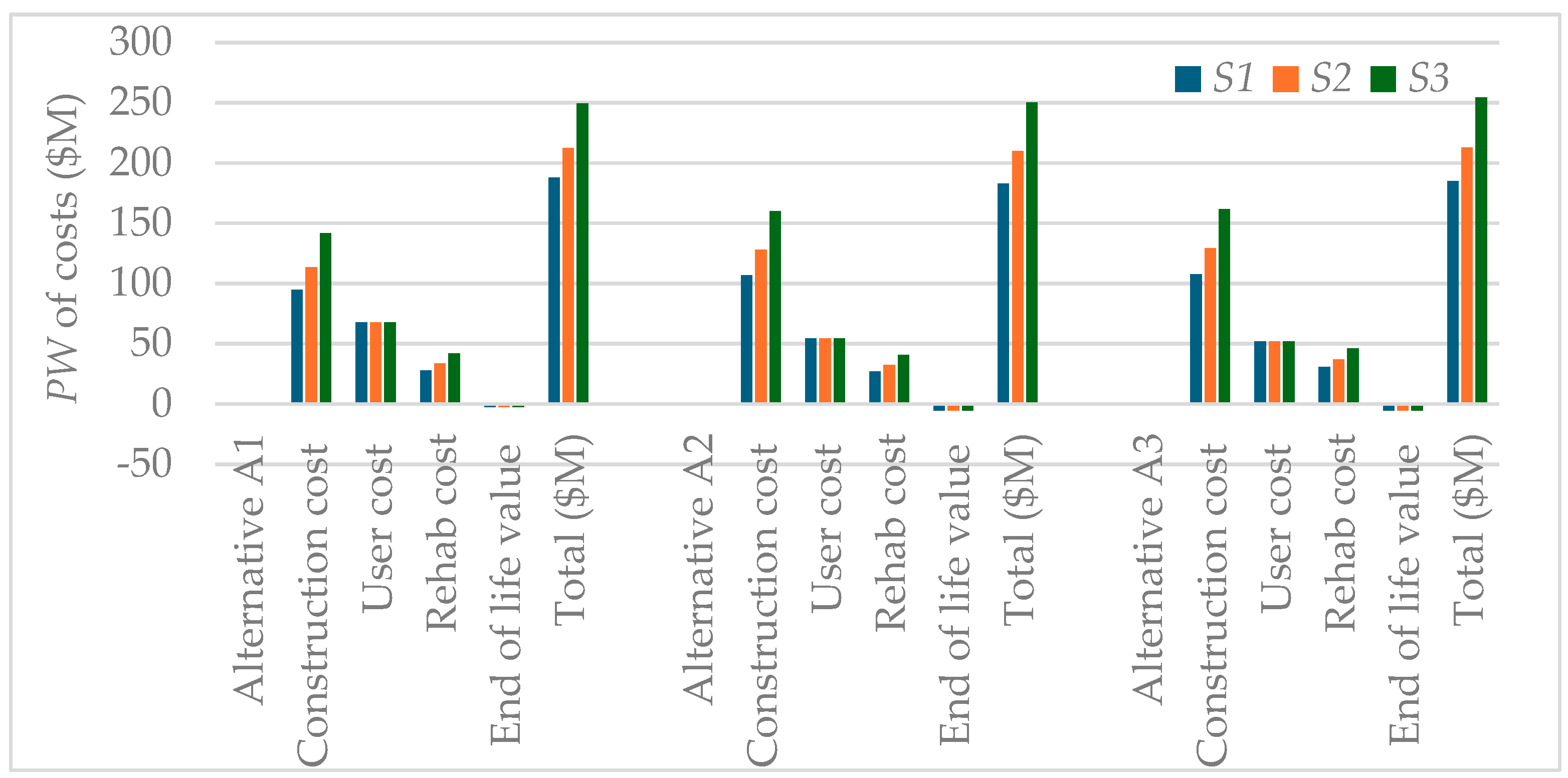
Figure 2.
Lifecycle net present worth (NPW) ($M) (2023 US$). Note: The NPW for A3-S3 combination is $0.05M. It is not visible due to scale effect.
Figure 2.
Lifecycle net present worth (NPW) ($M) (2023 US$). Note: The NPW for A3-S3 combination is $0.05M. It is not visible due to scale effect.
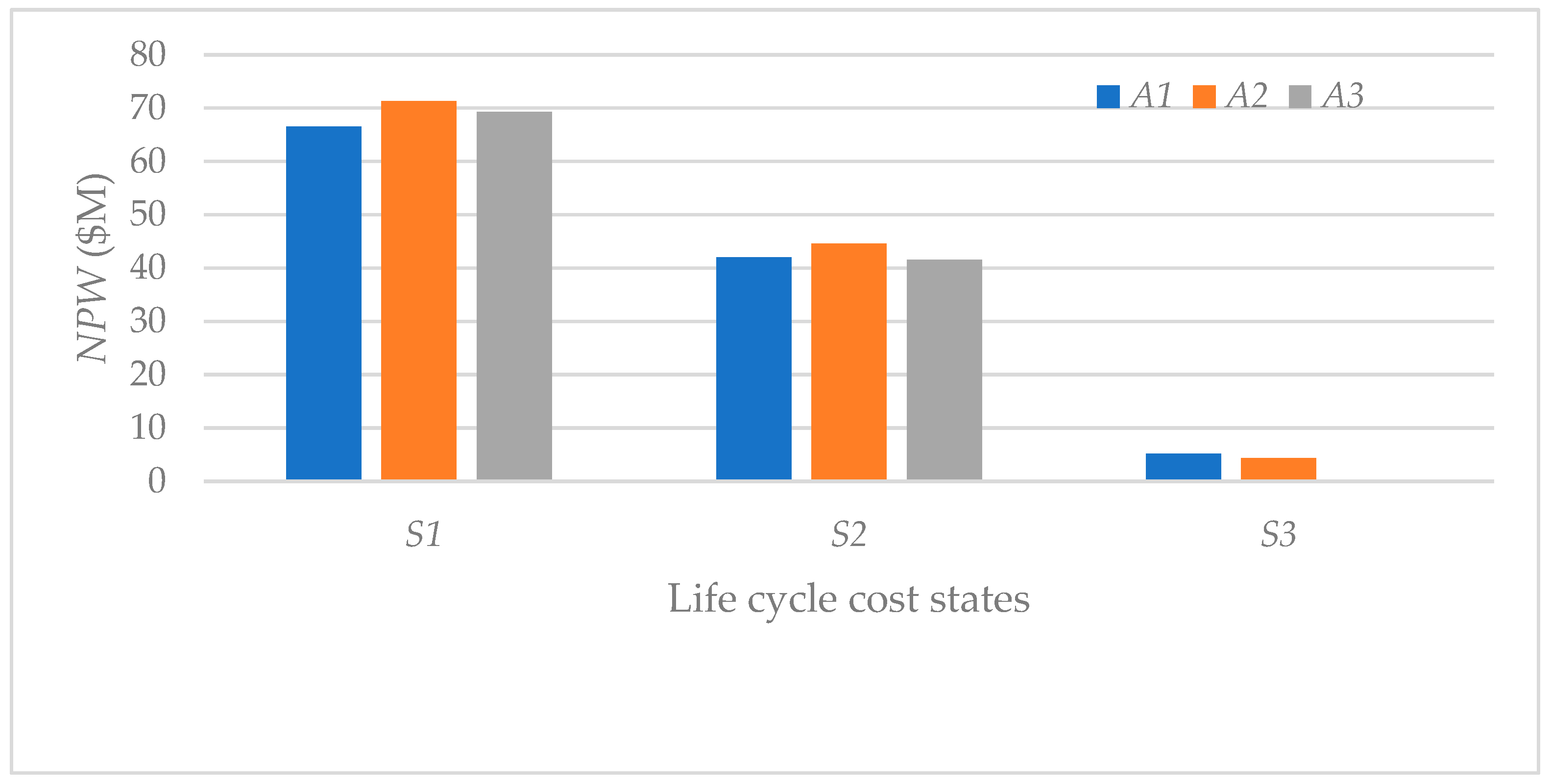
Figure 3.
Expected NPW results of risk analysis methods (2023$).
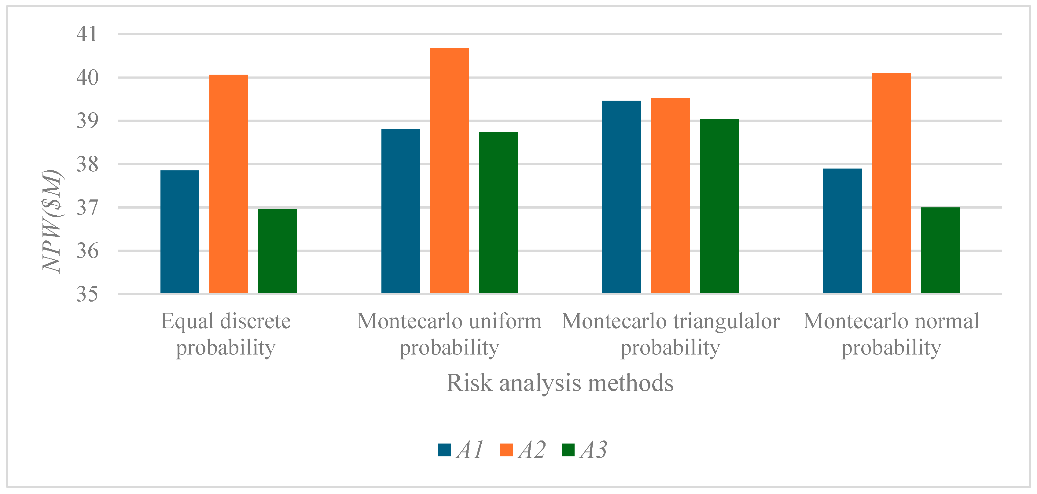
Figure 4.
Decision tree of pre-posterior information acquisition (Adapted from [35]).
Figure 4.
Decision tree of pre-posterior information acquisition (Adapted from [35]).
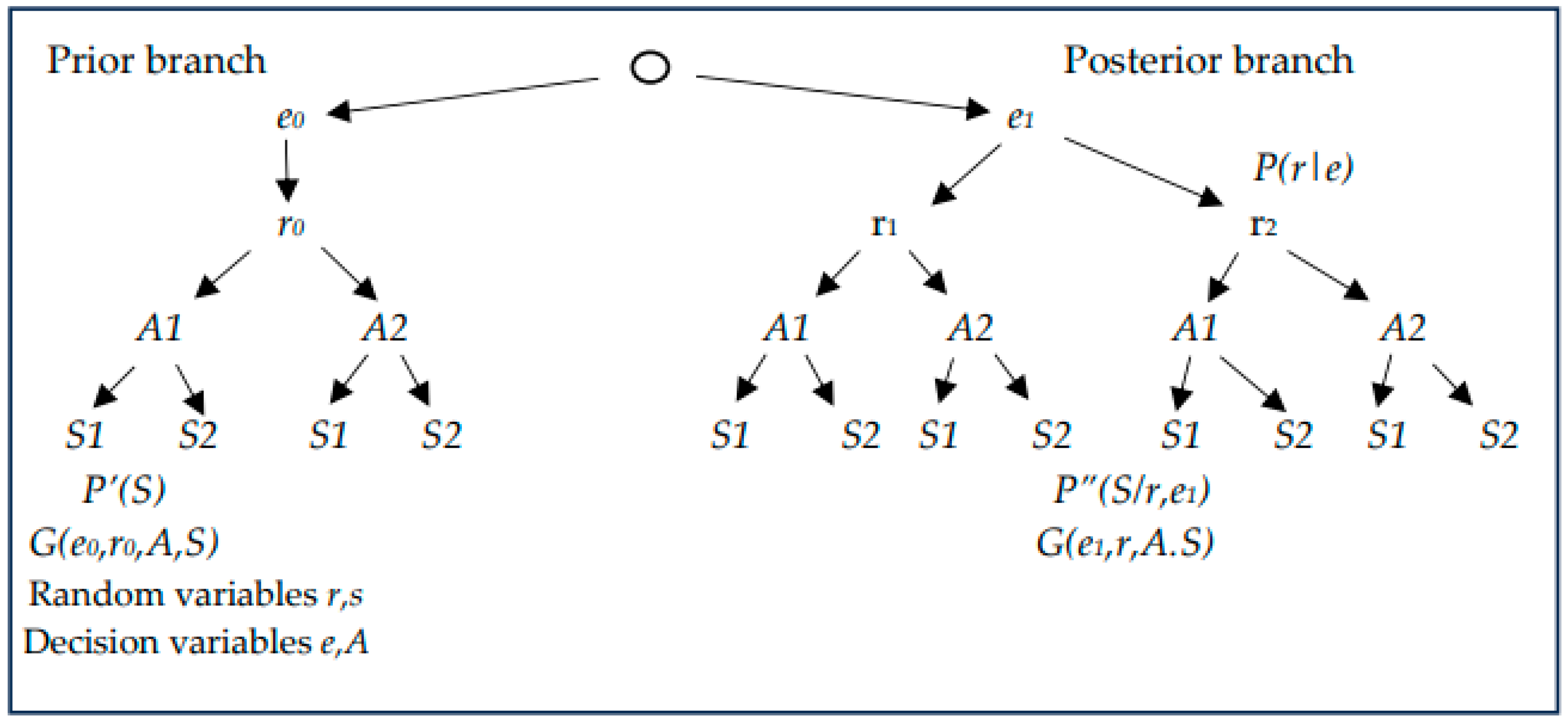
Figure 5.
Methodological steps in Bayesian pre-posterior analysis.
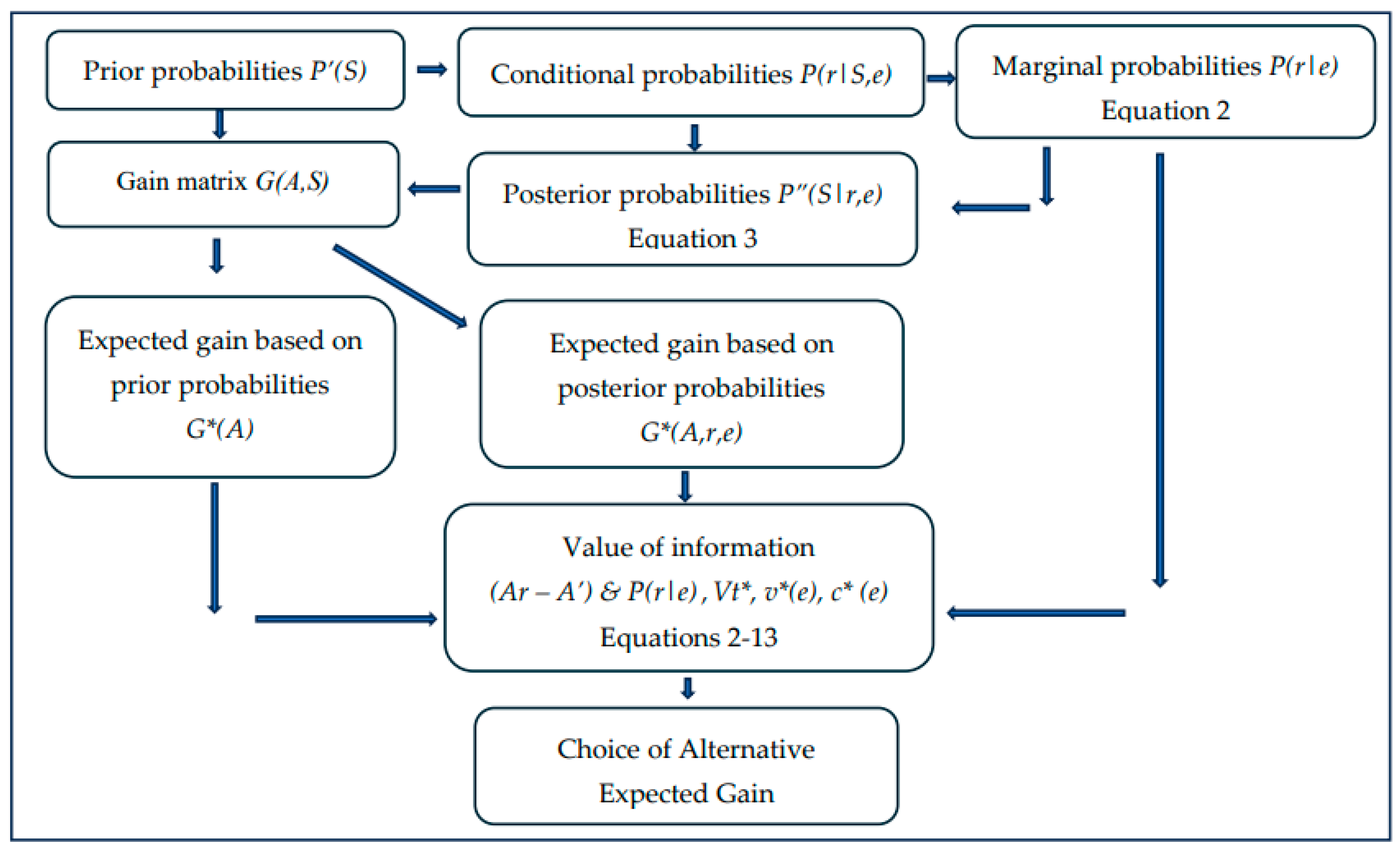
Figure 6.
Example 1 inputs, intermediate steps and outputs (2023$).
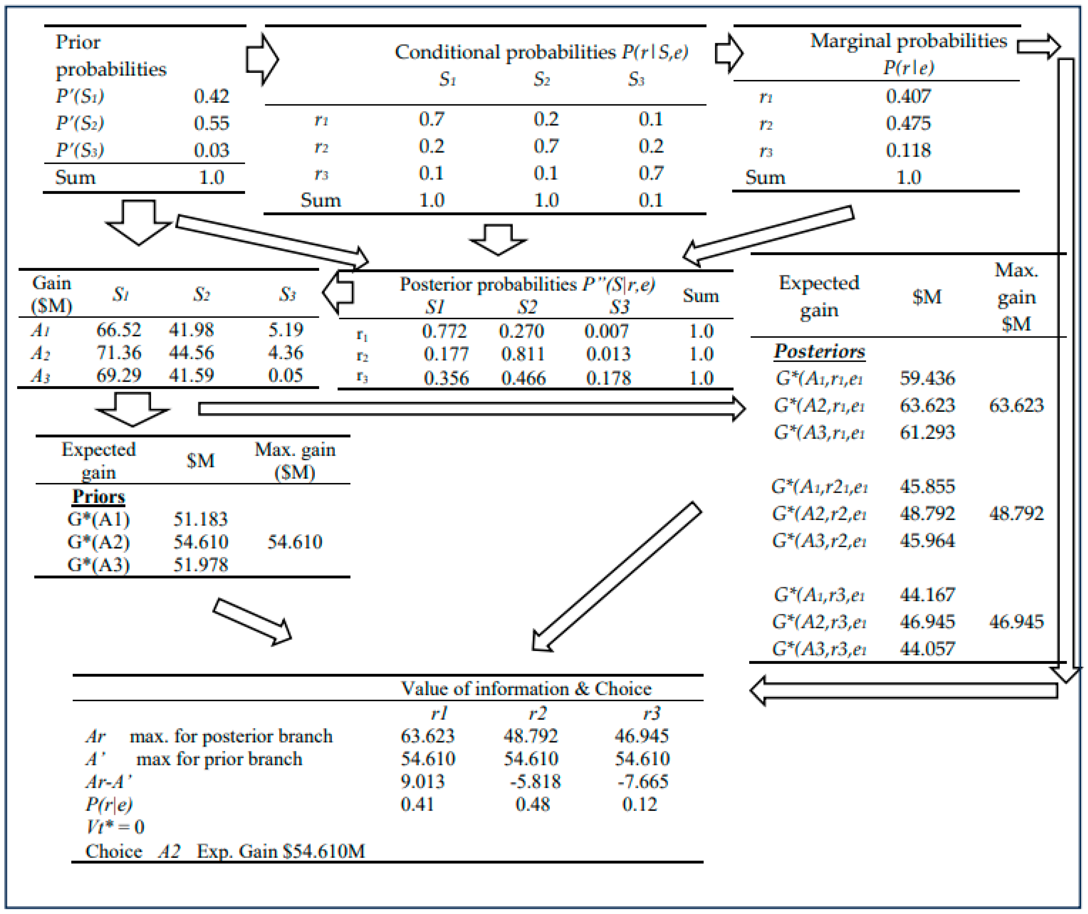
Figure 7.
Example 2 data and results (2023$).
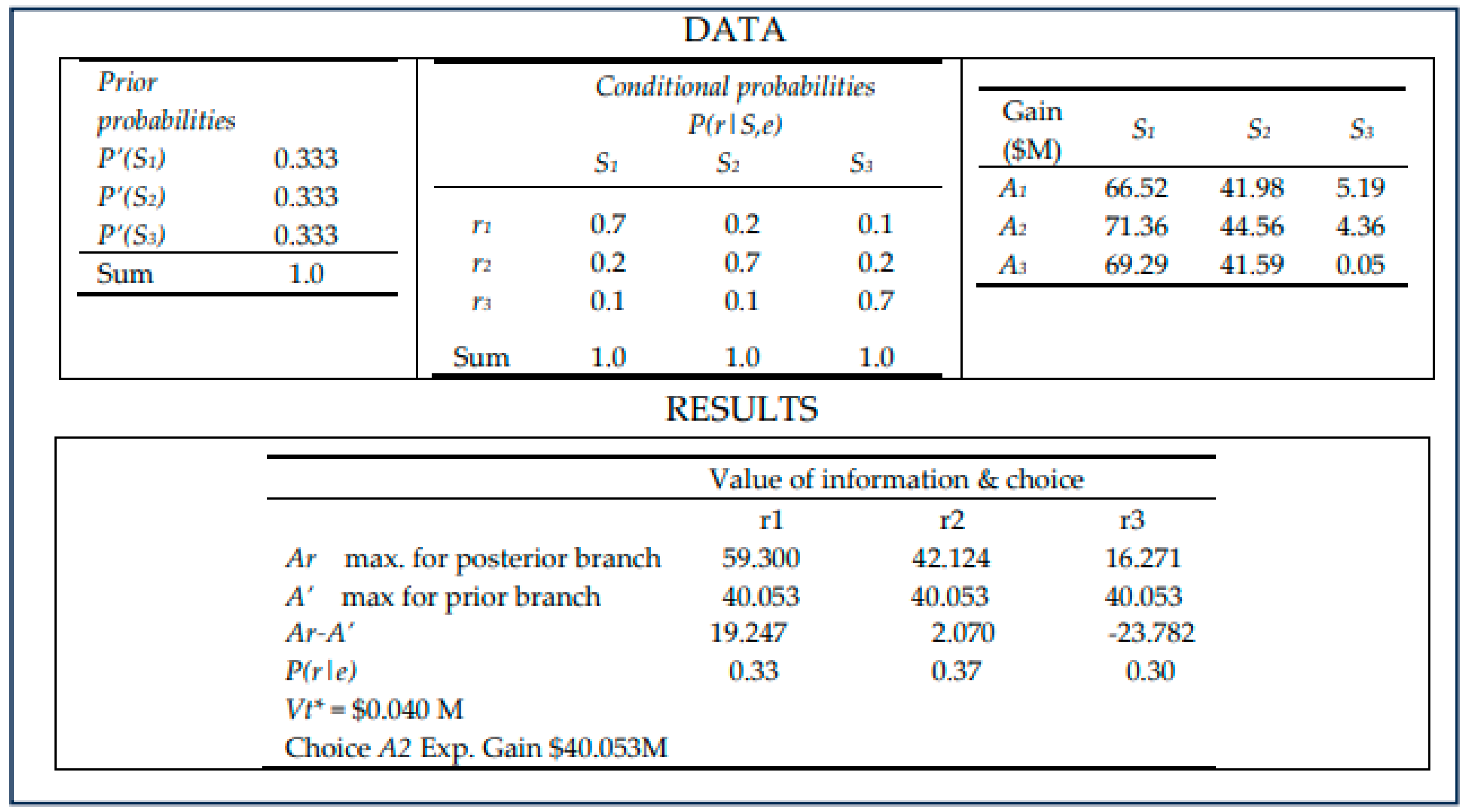
Figure 8.
Example 3 data and results (2023$).
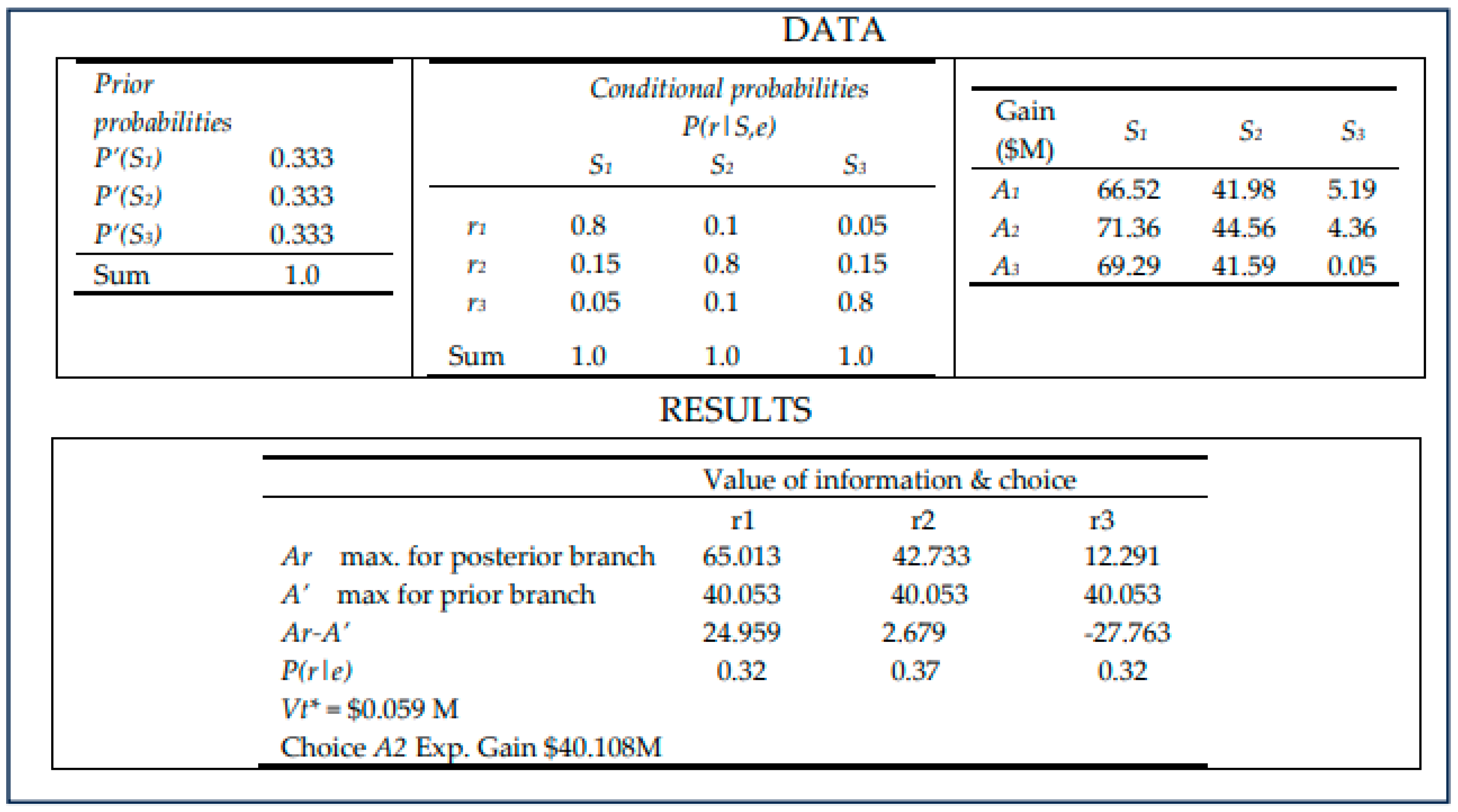
Figure 9.
Example 4 data and results (2023$).
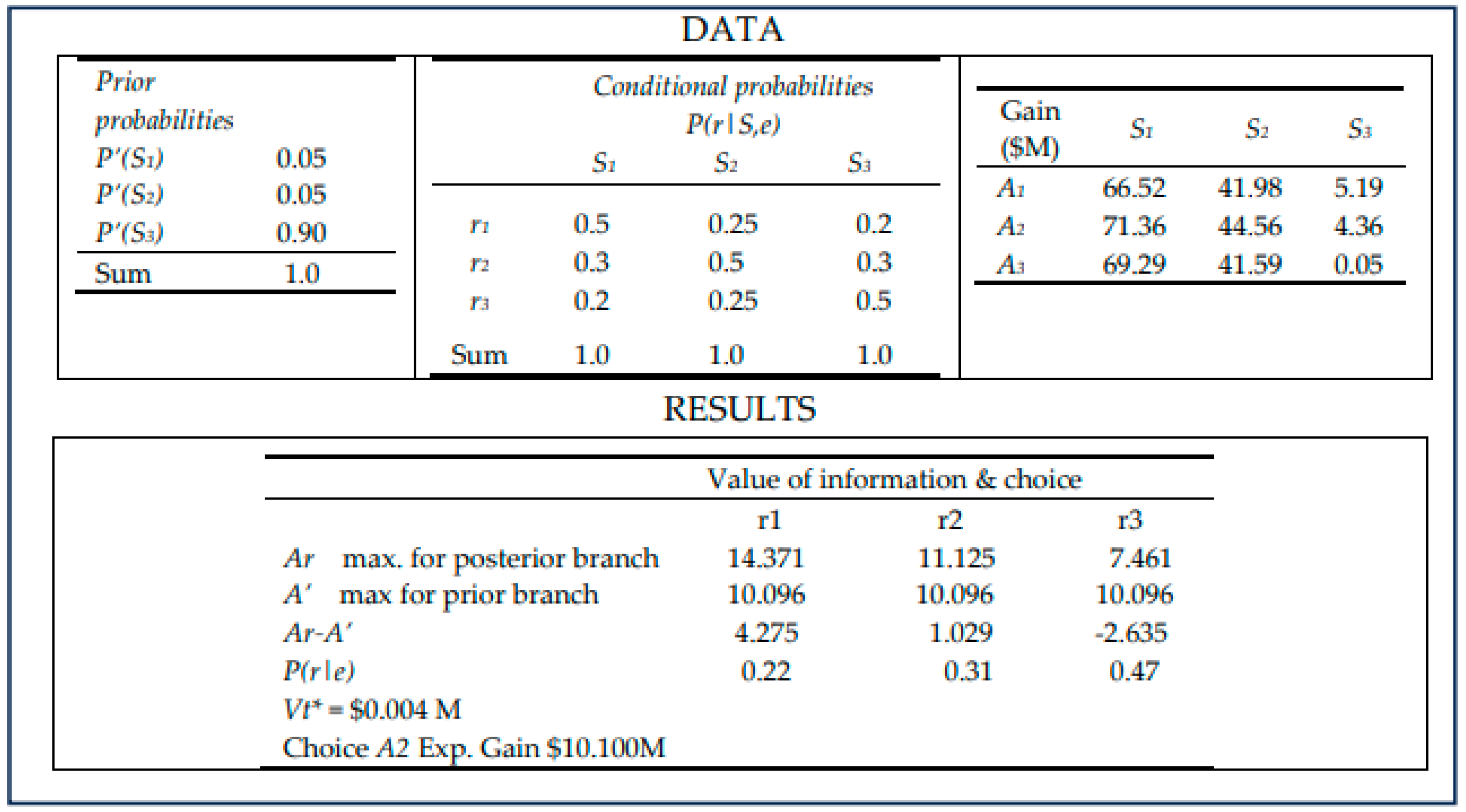
Figure 10.
Example 5 data and results (2023$).
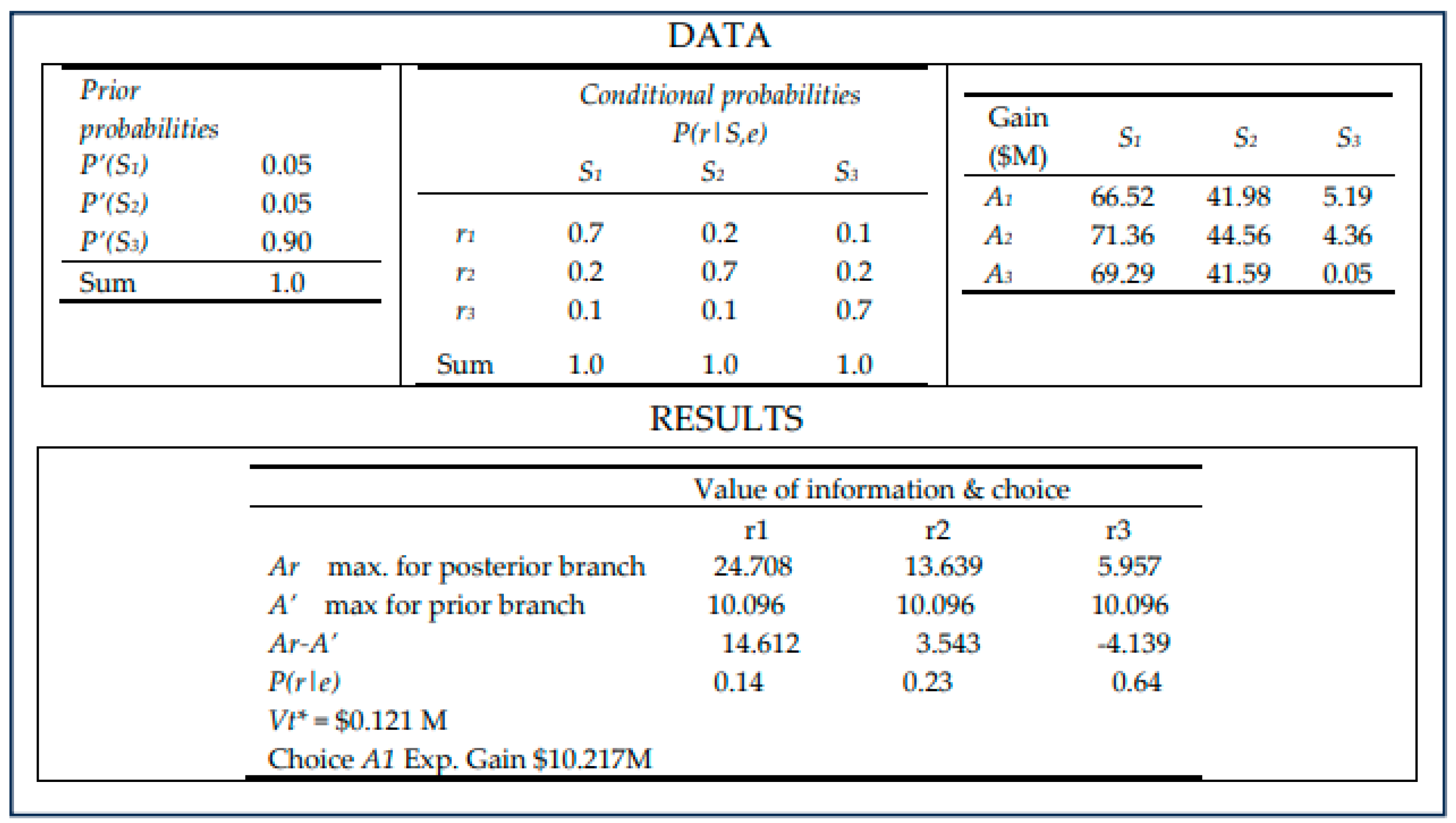
Figure 11.
Example 6 data and results (2023$).
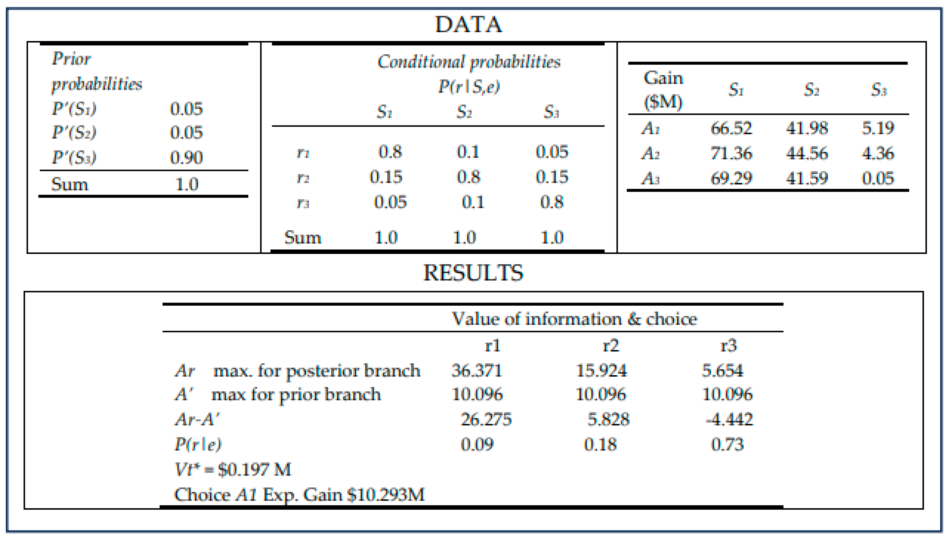
Figure 12.
Comparison of value of additional information (2023$).
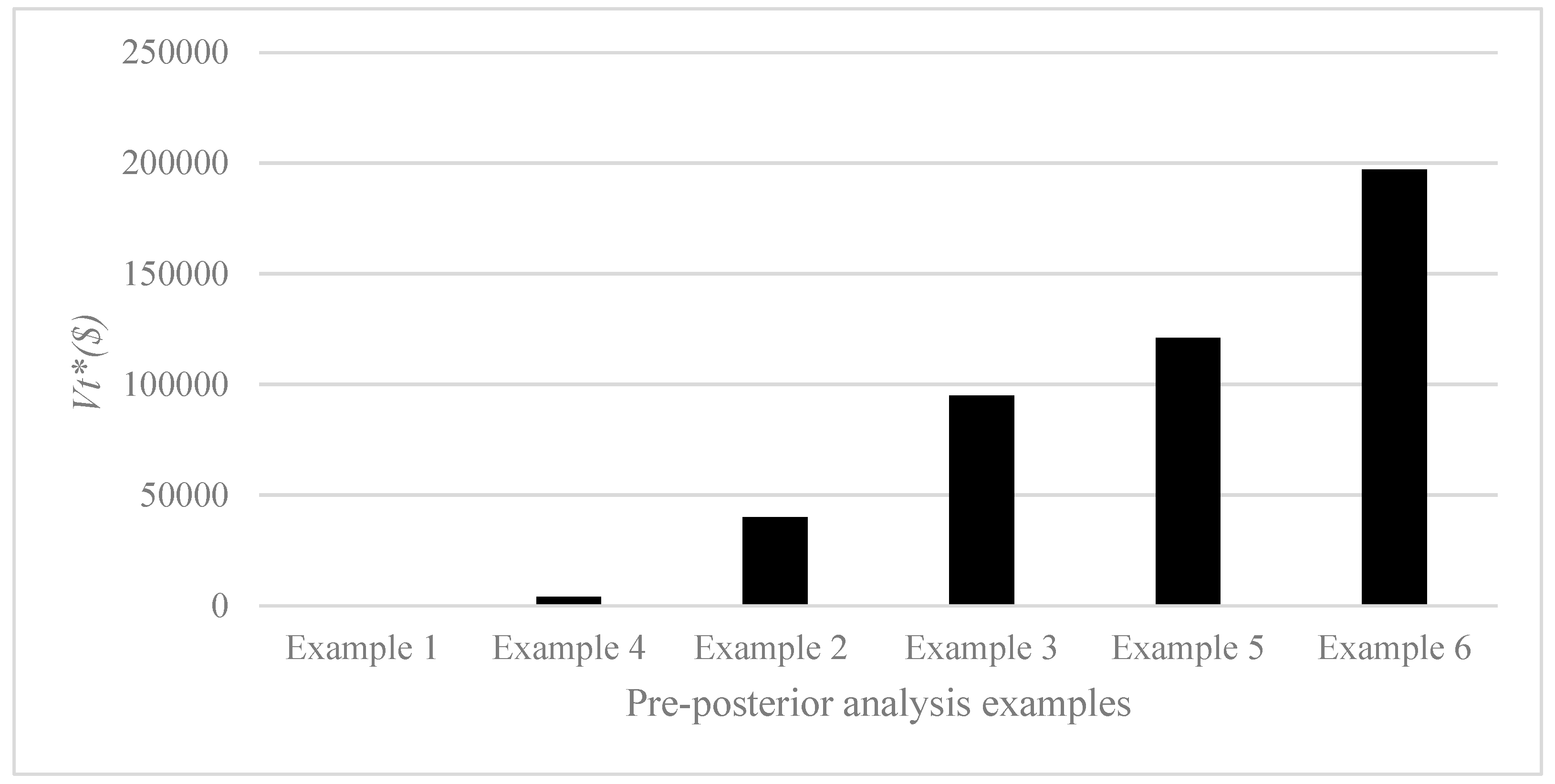

Table 1.
Sources of uncertainty in life cycle cost estimates and economic impacts.
| Life cycle cost component | Sources of uncertainty | Socio-economic impacts |
|---|---|---|
| Initial construction cost. |
Cost overruns potentially caused by many factors, including incomplete and/or design errors, and quality of data issues. |
|
| Cost of maintenance and rehabilitation cycles. |
Limitation of predictive models to forecast conditions under which service quality is delivered and associated cost of corrections. |
|
| User cost of congestion, safety, and vehicle operating cost. |
Uncertain traffic forecasts due to data and methodology issues. |
|
| End of life value (a negative cost) |
Predictive model limitation in producing end of life economic estimates. |
|
Table 2.
Lifecycle present worth (PW) of costs and net present worth ($M) (2023$).
| Alternative |
S1 PW(Costs) |
S2 PW(Costs) |
S3 PW(Costs) |
S1 NPW |
S2 NPW |
S3 NPW |
|---|---|---|---|---|---|---|
|
A1 A2 A3 |
187.88 183.04 185.11 |
212.42 209.84 212.81 |
249.21 250.04 254.35 |
66.52 71.36 69.29 |
41.98 44.56 41.59 |
5.19 4.36 0.05 |
Disclaimer/Publisher’s Note: The statements, opinions and data contained in all publications are solely those of the individual author(s) and contributor(s) and not of MDPI and/or the editor(s). MDPI and/or the editor(s) disclaim responsibility for any injury to people or property resulting from any ideas, methods, instructions or products referred to in the content. |
© 2025 by the authors. Licensee MDPI, Basel, Switzerland. This article is an open access article distributed under the terms and conditions of the Creative Commons Attribution (CC BY) license (http://creativecommons.org/licenses/by/4.0/).
Copyright: This open access article is published under a Creative Commons CC BY 4.0 license, which permit the free download, distribution, and reuse, provided that the author and preprint are cited in any reuse.


