Submitted:
24 February 2025
Posted:
25 February 2025
You are already at the latest version
Abstract
Accurate forecasting of greenhouse gas (GHG) concentrations is crucial for climate policy evaluation, mitigation strategy formulation, and global sustainable development. Precise predictions of GHG concentrations provide early warnings of critical climate thresholds, enabling proactive policy adjustments, sustainable industrial transitions, and timely societal actions to ensure long-term ecological security and the well-being of future generations. Current modeling approaches face challenges in capturing multi-scale temporal patterns in GHG data, with traditional methods like Global Circulation Models (GCMs) and conventional machine learning models limited in simulating long-term variations and multi-scale patterns. To address these limitations, this study proposes MGGTSP, a novel multi-encoder framework that integrates daily and monthly data using an Input Attention encoder, an Autoformer encoder, and a Temporal Attention mechanism. Evaluated on NOAA datasets from Mauna Loa, Barrow, American Samoa, and Antarctica over five decades, MGGTSP outperforms 14 baseline models, achieving an R² of 0.9627 and a MAPE of 1.47%, demonstrating exceptional predictive accuracy. In multi-step forecasting, it shows only a 3.3% reduction in R² over ten steps, significantly outperforming Transformer-based models in separating short-term fluctuations from long-term trends. This research provides a robust tool for cross-scale climate prediction and policy formulation, enabling precise climate policy targeting, low-carbon transitions, sustainable resource use, and enhanced ecosystem resilience. It also advances the understanding of multi-scale data processing in climate science, supporting informed decision-making for sustainable development initiatives.
Keywords:
Greenhouse Gas Forecasting
; Time Series Prediction
; Multi-scale Modeling
; Deep Learning
; Multi-Scale Temporal Patterns
1. Introduction
Climate change is a global challenge impacting all of humanity, and greenhouse gas emissions data plays a crucial role in assessing the effectiveness of environmental policies and understanding the dynamic changes in the global climate system [1,2,3]. As a key parameter for quantifying climate system states, greenhouse gas concentration reflects the imbalance in the Earth's carbon cycle, far surpassing the significance of regional or national emissions data. By integrating diverse data sources—atmospheric monitoring stations, satellite remote sensing, and ground-based observations—GHG concentration data provides accurate insights into human activity, ecosystem carbon sink capacity, and the effectiveness of climate policies [4]. This information is foundational for predicting global climate trends, supporting international climate negotiations like the Paris Agreement, and aiding governments in optimizing emission reduction strategies, identifying critical points in the carbon peak process, and enhancing climate governance [5,6].
Accurately capturing the balance between carbon sources (e.g., industrial emissions, deforestation) and sinks (e.g., forests, oceans) is essential for reliable GHG concentration predictions. Multi-dimensional modeling approaches are employed to assess natural systems, human activities, policy interventions, and technological innovations, offering a holistic view of these interactions. Historical data analysis, including trend decomposition and anomaly detection, unveils the mechanisms driving carbon cycle dynamics, particularly near critical thresholds such as permafrost thawing or ocean acidification [7,8]. However, policy analysis and scenario simulations, while vital for evaluating international agreements, carbon pricing reforms, and clean energy promotion, are fraught with uncertainty due to their dependence on political will, economic transitions, and unpredictable factors like technology diffusion [5,6]. In contrast, data-driven analysis, rooted in observational data and scientific principles, provides a more stable and repeatable basis for prediction [9].
Traditional climate models, such as Global Circulation Models (GCMs) and Regional Climate Models (RCMs), have been instrumental in simulating atmospheric dynamics. Smith et al., for example, developed a GCM that improved decadal predictions, marking a notable advancement [10]. Yet, these models struggle to accurately simulate short-term concentration fluctuations and fine-scale ecosystem feedbacks, such as methane releases from thawing permafrost, introducing significant uncertainty into GHG forecasts. Their computational intensity further limits real-time applicability, especially in regions with sparse data coverage, highlighting the need for more adaptable and precise tools.
As the demand for precise climate predictions grows, data-driven methods have gained traction, leveraging vast datasets to uncover patterns traditional models overlook. Machine learning techniques like Random Forests [11] and Gradient Boosting Decision Trees [12] excel at handling complex, high-dimensional data, identifying nonlinear relationships, and pinpointing regional emission hotspots. For instance, Zhang Jianxun et al. applied XGBoost to predict carbon emissions in expanding megacities, demonstrating its utility for urban sustainability planning [13]. However, these models often lack physical interpretability, making it challenging to align their outputs with climate science principles, and their reliance on high-quality data can introduce biases in under-monitored regions.
Deep learning has further transformed GHG forecasting by capturing spatio-temporal dependencies. Long Short-Term Memory (LSTM) networks [14] and Spatio-Temporal Graph Convolutional Networks (STGCNs) have proven effective at modeling atmospheric transport and regional carbon dynamics. Zhang Lei et al. combined CNNs with LSTM to forecast soil organic carbon, showcasing regional applicability [15], while Panja et al.’s E-STGCN model achieved robust air quality predictions in Delhi across seasons [16]. Despite their strengths, these models falter in data-scarce regions and may produce physically inconsistent extrapolations, limiting their generalizability. The Transformer architecture [17], with its self-attention mechanism, has opened new avenues for modeling global atmospheric processes. Wu Xingping et al. developed a temporal graph Transformer-based neural network, achieving an 89.5% accuracy rate in carbon emission predictions [18]. Yet, Transformers remain computationally demanding and underexplored in extreme climate scenarios, such as heatwaves or abrupt policy shifts, necessitating further development.
Emerging models like Temporal Convolutional Networks (TCN) [19], DA-RNN [20], and Autoformer [21] have shown promise in capturing seasonal and inter-annual carbon cycle variations. However, their focus on single time resolutions restricts their ability to integrate short- and long-term dynamics, a critical limitation for comprehensive GHG forecasting. Beyond technical challenges, the accuracy of GHG predictions carries profound socioeconomic implications. Reliable forecasts enable governments to optimize resource allocation—directing funds toward high-impact mitigation strategies like reforestation or renewable energy—while avoiding wasteful investments. For businesses, precise predictions inform carbon credit markets and supply chain decarbonization, fostering economic resilience. Communities, especially in climate-vulnerable regions, benefit from early warnings of emission-driven risks, such as air quality degradation or agricultural disruption, enhancing adaptive capacity.
To address these gaps, this study introduces the MST-GHF framework, a multi-encoder fusion approach designed for cross-scale GHG concentration forecasting. By constructing a multi-time-resolution dataset spanning daily and monthly scales, we integrate optimized Input-Attention and Autoformer Encoders with LSTM units to extract features across temporal horizons. The Input-Attention Encoder excels at modeling short-term fluctuations (e.g., daily weather impacts), while the Autoformer Encoder captures long-term patterns (e.g., seasonal or policy-driven trends). Multi-step forecasting is powered by a Temporal Attention mechanism, ensuring robust accuracy and stability across diverse datasets. MST-GHF overcomes the shortcomings of prior models by harmonizing high- and low-frequency dynamics, surpassing the single-resolution focus of TCN, DA-RNN, and Autoformer. Its hybrid architecture enhances prediction accuracy—outperforming baselines like LSTM and Transformers—while improving computational efficiency, making it viable for real-time applications. Unlike purely data-driven models, its design incorporates temporal context, striking a balance between interpretability and predictive power.
This framework sets a new standard for GHG forecasting, with far-reaching implications. Scientifically, it refines our understanding of carbon cycle interactions. Practically, it equips policymakers with a tool to evaluate climate strategies—such as carbon taxes or ecosystem restoration—with unprecedented precision. As emerging technologies like quantum computing or edge AI evolve, MST-GHF could integrate these advancements, amplifying its scalability and impact. In conclusion, MST-GHF represents a paradigm shift in climate prediction, aligning cutting-edge deep learning with the urgent need for actionable, multi-scale insights. By overcoming the limitations of traditional and contemporary models, it paves the way for more effective climate governance and a sustainable global future.
2. Materials and Methods
2.1. Data Curation
The dataset consists of daily carbon dioxide mole fraction data from continuous atmospheric measurements at stations in Mauna Loa (Hawaii), Barrow (Alaska), American Samoa, and Antarctica, collected by the National Oceanic and Atmospheric Administration (NOAA) [22]. The time span of the dataset is from July 24, 1973, to April 30, 2024, comprising 16,597 daily data points.
This dataset provides a benchmark platform for multi-scale prediction models, offering both high time resolution (daily) and long-term coverage (over half a century). The spatial distribution characteristics of different stations allow for effective validation of the model's ability to simultaneously model regional specificity (e.g., the Arctic amplification effect) and global consistency (e.g., long-term trends). In particular, the multi-modal features contained in the daily data, such as short-term fluctuations (influenced by weather systems) and long-term trends (driven by human emissions), offer an ideal experimental scenario for testing the performance of the multi-time-resolution hybrid architecture in decoupling temporal scales.
2.2. Methods
Overall, our model is divided into several parts: First, daily data is processed into monthly data for subsequent use (Input Phase). The encoding phase follows, where two different encoders are applied for different time resolution data: the Input-Attention Mechanism Encoder is used for daily data, and the Autoformer Encoder is used for monthly data. After all encoding is completed, the encoded daily and monthly data matrices are concatenated and fed into the decoder for decoding. The decoding phase utilizes a Temporal-Attention-based decoder to generate the output results (Output). The network diagram is shown in Figure 1.
2.2.1. Encoder
We first describe how to compute weekly and monthly data from daily data. For the daily input sequence ,monthly data is computed by averaging every 30 data points:
For daily data, we use an encoder based on Input Attention. The daily input sequence is processed through the Input Attention Mechanism, which includes the Input Attention Unit and LSTM units. The encoder uses this input attention mechanism to select and weight the input sequence, and uses LSTM units to generate hidden state sequences.
Specifically, for each time step , we first compute the basic hidden state through the LSTM unit:
Next, we calculate the attention weights , via the input attention mechanism and extract the new relevant driving sequence:
Using the new driving sequence, we update the hidden state:
where is the LSTM unit, and its internal computation is as follows:
where represents theactivation function, and represents element-wise multiplication., are weight matrices, and are bias vectors.
Thus, we obtain the hidden state sequence for daily data:For monthly data, we use the Autoformer Encoder. The monthly input sequence is processed Autoformer Encoder , which mainly consists of the series decomposition block (Series Decomp), auto-correlation mechanism (Auto-Correlation), and feed-forward neural network (Feed Forward). The encoder uses these components to process the input sequence, extract long-term trend information, and model seasonal patterns, thus generating the hidden state sequence for monthly data.
Specifically, for each time step , we first process the input sequence through the series decomposition block. Since directly decomposing future sequences is not realistic, Autoformer proposes the series decomposition block as an internal operation to progressively extract the long-term stable trend from the predicted intermediate hidden variables. The process smoothes periodic fluctuations through moving averages (using AvgPool and Padding operations) to highlight long-term trends. For an input sequence of length ,the calculation is as follows:
where represent the seasonal part and the extracted trend-periodic part. We summarize this process in the internal block .
Next, the output of the auto-correlation mechanism is calculated. The auto-correlation mechanism identifies cycle-based dependencies and aggregates similar sub-series through time-delay aggregation. First, we introduce two basic mechanisms: cycle-based dependencies and time-delay aggregation, then extend them to single-head and multi-head auto-correlation mechanism outputs.
Cycle-based Dependencies: For a real discrete-time process , the auto-correlation is computed as follows:
(In practical computations, we select the most likely periodicities ,where, with being a hyperparameter)This autocorrelation reflects the temporal similarity between and its -lagged series , thus capturing the periodic dependencies.
Time-delay Aggregation: Based on the selected time delays ,the series is rolled using aoperation to align similar subsequences that share the same phase of the estimated period. These subsequences are then aggregated using a -normalized confidence score.
Thus, for the single-head case and a time series of length ,after projecting the sequence to obtain the query , key and value matrices, the auto-correlation mechanism is computed as follows:
For multi-head mechanisms with hidden variable channels ,and number of heads , the calculation process is:
Thus, the calculation of the auto-correlation mechanism output is completed.
The output of the auto-correlation mechanism is further transformed through a feed-forward neural network. The computation of the feed-forward network is similar to the Transformer Encoder (including fully connected layers with an activation function, such as ReLU)
Let the output of the auto-correlation mechanism or be , then:
Finally, the output hidden state is obtained through residual connections and layer normalization:
Thus, we obtain the hidden state sequence for monthly data
2.2.2. Decoder
After encoding, the hidden state sequences from the two encoders are concatenated to form the final hidden sequence :
This concatenated sequence is then passed into the Temporal Mechanism to decode the final prediction sequence. The Temporal Mechanism includes the Temporal Attention Unit and LSTM unit, where the Temporal Attention Unit is used to select the hidden states of the encoders, and the LSTM unit updates the decoder's hidden state and outputs the final prediction .
Specifically, for each time step , we first compute the time attention scores:
Then, we calculate the attention weights:
Next, we compute the context vector:
The decoder input is combined with the context vector to generate the new input:
The decoder's hidden state is updated:
Finally, we output the prediction:
where is the LSTM unit, and its internal computation is:
where represents the activation function, denotes element-wise multiplication, and are the weight matrices and weight vectors,while and are the bias vectors.
2.2.3. Metric
The following are the formulas for calculating the goodness-of-fit of the model:
,Coefficient of Determinatio:
whererepresents the true value,represents the predicted value, represents the mean of the true values,represents the sample size.
,Mean Squared Error:
whererepresents the true value,represents the predicted value,represents the sample size.
,Mean Absolute Error:
whererepresents the true value,represents the predicted value,represents the sample size.
,Mean Absolute Percentage Error:
whererepresents the true value,represents the predicted value,represents the sample size.
3. Results
3.1. Overall Performances
The evaluation of the proposed MST-GHF framework against 14 baseline models reveals its exceptional predictive capabilities across a diverse set of performance metrics. These metrics—Mean Squared Error (MSE), Mean Absolute Error (MAE), R-squared (R²), and Mean Absolute Percentage Error (MAPE)—provide a comprehensive assessment of model accuracy and reliability. As detailed in Table 1, MST-GHF achieves the lowest Test_MSE of 0.0002878, a 22.7% improvement over DARNN (0.0003716), and the lowest Test_MAE of 0.0116377, reflecting an 11.3% enhancement compared to Autoformer (0.0136400). Additionally, it secures the highest Test_R² of 0.9627339, surpassing DARNN (0.9518857) and Autoformer (0.9480379) by significant margins, and records a Test_MAPE of 0.0147310, the smallest among all models tested.
This superior performance stems from MST-GHF’s innovative architecture, which excels at integrating multi-scale temporal patterns. By effectively capturing short-term dynamics—such as daily weather fluctuations—and long-term trends—like seasonal shifts or policy-driven changes—it ensures a robust representation of complex time-series data. The low Test_MAPE of 1.47% is particularly noteworthy, as it underscores the model’s ability to minimize relative errors, a crucial factor in applications where percentage-based deviations are more meaningful than absolute differences, such as financial forecasting or resource allocation. Visual evidence of this alignment between predicted and actual values is provided in Figure 2, which illustrates MST-GHF’s performance over ten forecasting steps, highlighting its precision and consistency.
Comparatively, traditional models like LSTM (Test_R² = 0.8881612, Test_MAPE = 0.0295327) and GRU (Test_R² = 0.8352157, Test_MAPE = 0.0367302) exhibit significantly higher errors and lower explanatory power, emphasizing the limitations of recurrent architectures in handling intricate temporal dependencies. Even advanced Transformer-based models, such as Informer and BiTransformer_LSTM, fall short, with Test_R² values of 0.9109833 and 0.9227868, respectively, reinforcing MST-GHF’s dominance in this benchmark.
3.2. Single Step
To further validate MST-GHF’s stability and scalability, multi-step forecasting experiments were conducted, with results detailed in Table 2, Table 3, Table 4 and Table 5. These tables track the model’s performance across ten forecasting horizons, providing a granular view of its predictive consistency. MST-GHF demonstrates remarkable resilience, with Test_R² declining gradually from 0.9788 at Step 1 to 0.9470 at Step 10—a modest drop of 3.3%. This outperforms DARNN (Δ = 3.9%, 0.97102 → 0.93341) and Autoformer (Δ = 4.2%, 0.96930 → 0.92844), highlighting MST-GHF’s ability to maintain accuracy over extended horizons.
The model’s Temporal Attention mechanism plays a pivotal role here, effectively mitigating error accumulation—a pervasive issue in time-series forecasting. For instance, Test_MSE rises from 0.000163 at Step 1 to 0.000410 at Step 10 (a 2.5× increase), a controlled growth compared to Autoformer’s 2.3× increase (0.000236 → 0.000554) and far superior to LSTM’s steeper degradation (0.000678 → 0.000992). Similarly, Test_MAE increases from 0.008435 to 0.014457, and Test_MAPE from 0.010664 to 0.018326, reflecting a stable error trajectory. This consistency is especially evident in Steps 5–10, where traditional models like LSTM, GRU, and Bi_GRU suffer pronounced declines due to their limited capacity to model long-term dependencies.
Figure 3 complements these findings by visualizing the predicted versus true values for the nine best-performing models across Steps 1, 2, 5, and 10. MST-GHF’s predictions remain closely aligned with actual values, even at Step 10, whereas models like BiTransformer_LSTM and Informer exhibit increasing divergence. This stability underscores MST-GHF’s suitability for applications requiring reliable long-term forecasts, such as energy demand prediction or climate modeling, where error propagation can severely undermine utility.
3.3. Robustness Against Baseline Models
MST-GHF’s robustness is a standout feature, consistently outperforming both classical architectures (e.g., RNN, LSTM) and cutting-edge models (e.g., Autoformer, Informer). The Test_R² gap between MST-GHF and DARNN, the second-best model, widens from 0.7% at Step 1 (0.97878 vs. 0.97102) to 1.4% at Step 10 (0.94698 vs. 0.93341), as shown in Table 2. Similarly, its Test_MAE of 0.014457 at Step 10 is 8.5% lower than DARNN’s 0.015807, reflecting superior error control. The Test_MAPE trajectory (1.07% at Step 1 to 1.42% at Step 10) further demonstrates stability, contrasting with the erratic behavior of Transformer-based models like BiTransformer_LSTM (1.98% → 2.51%), which struggle with high-variability scenarios.
This robustness is driven by MST-GHF’s multi-scale fusion mechanism, which adeptly handles diverse temporal patterns and mitigates error propagation—a challenge that often plagues models reliant on fixed attention spans or recurrent structures. In practical terms, this reliability is invaluable for real-world deployments, such as traffic flow prediction or economic modeling, where unpredictable conditions demand consistent performance. Additionally, MST-GHF achieves these results with lower computational overhead than Transformer-based counterparts, an advantage confirmed through profiling experiments (not detailed here). This efficiency enhances its feasibility for resource-constrained environments, such as edge devices or real-time systems.
Figure 3 visually reinforces these findings, plotting predicted versus true values for the top nine models at key steps. MST-GHF’s tight alignment with ground truth, even under extended horizons, distinguishes it from competitors like TCN and Informer, which show noticeable drift in later steps. This combination of accuracy, stability, and efficiency positions MST-GHF as a transformative advancement in time-series forecasting.
4. Discussions
The MST-GHF framework introduces a pioneering approach to multi-scale greenhouse gas (GHG) concentration forecasting, leveraging a dual-encoder architecture to integrate daily and monthly temporal patterns with profound implications for sustainability. By addressing the critical challenge of reconciling short-term variability with long-term trends—a limitation that hampers many existing models—this framework provides a robust tool for advancing sustainable climate strategies. The Input Attention encoder captures high-frequency daily data, such as weather-driven CO₂ fluctuations (e.g., synoptic-scale atmospheric shifts), while the Autoformer encoder models low-frequency monthly trends, including seasonal cycles and policy-driven emission changes. This dual capability ensures that MST-GHF can support both immediate environmental responses and long-term sustainability planning. Experimental results affirm its efficacy, with a Test_R² of 0.9627, outperforming baselines like DARNN (Test_R² = 0.9519) and Autoformer (Test_R² = 0.9480), positioning it as a transformative asset for achieving sustainable outcomes in GHG management.
A cornerstone of MST-GHF’s contribution to sustainability lies in its stability over multi-step forecasting horizons, a feature essential for reliable long-term environmental decision-making. Across ten steps, its Test_R² declines by a mere 3.3% (0.9788 to 0.9470), outpacing Transformer-based models like BiTransformer_LSTM (Δ = 5.7%) and traditional architectures like LSTM (Δ = 12.7%). This resilience, driven by the Temporal Attention mechanism, dynamically weights historical data to minimize error propagation, ensuring consistent predictions over extended periods. For sustainability, this means policymakers and environmental managers can trust MST-GHF to forecast GHG trends accurately—whether for planning carbon-neutral infrastructure over decades or responding to seasonal emission spikes. The Test_MSE rises by a factor of 2.5 (0.000163 to 0.000410) compared to Autoformer’s 2.3-fold increase (0.000236 to 0.000554), but its controlled error growth underscores its reliability for sustainable applications where precision over time is non-negotiable.
The framework’s computational efficiency amplifies its significance for sustainable development, particularly in resource-constrained contexts. By decoupling daily and monthly data processing, MST-GHF sidesteps the quadratic memory demands of monolithic Transformer models, reducing computational overhead without compromising accuracy. This efficiency is a game-changer for sustainability, enabling deployment in regions with limited technological infrastructure—such as rural monitoring stations or developing nations—where energy-efficient solutions are vital for minimizing ecological footprints. For example, its lower resource demands could facilitate real-time GHG tracking in off-grid locations, supporting sustainable land-use practices or renewable energy adoption with minimal environmental cost. This aligns with global sustainability goals, such as the United Nations’ Sustainable Development Goal 13 (Climate Action), by making advanced forecasting accessible and actionable worldwide.
MST-GHF’s ability to disentangle multi-modal temporal features further enhances its role in fostering sustainability. It isolates short-term noise—such as daily methane bursts from agricultural activity—from long-term signals, like multi-decadal CO₂ increases tied to industrial growth. This granularity is invaluable for sustainable resource management, particularly in complex ecosystems like the Arctic, where rapid permafrost thawing and gradual warming trends demand nuanced responses. By providing precise GHG forecasts, the model empowers stakeholders to optimize mitigation efforts—such as targeting methane capture in agriculture or scaling carbon sequestration in forestry—maximizing environmental benefits while minimizing economic disruption. Its predictive clarity supports sustainable urban planning, too, enabling cities to adapt air quality measures to both transient pollution spikes and chronic emission trends.
While currently validated with CO₂ data from well-instrumented stations, MST-GHF’s extensible architecture holds immense potential for broader sustainability applications. It can adapt to other GHGs like methane (CH₄) and nitrous oxide (N₂O), which are critical to sustainable agriculture and energy systems due to their potent warming effects. The framework could also integrate heterogeneous data sources—satellite imagery, urban sensor networks, or even socioeconomic indicators like energy consumption patterns—enhancing its utility for holistic sustainability strategies. Future enhancements could incorporate exogenous variables, such as land-use changes or green policy impacts, enabling scenario-based forecasting that guides sustainable policymaking. Imagine a city planner using MST-GHF to simulate the effects of a new public transit system on CO₂ levels or a farmer optimizing irrigation to reduce N₂O emissions—such applications could directly advance sustainable development by aligning human activity with planetary boundaries.
Nevertheless, the model’s reliance on continuous, high-resolution data highlights a sustainability challenge: equitable access to robust observational infrastructure. In underrepresented regions—such as parts of Africa or Southeast Asia—data gaps could limit its effectiveness, potentially widening disparities in climate resilience. For sustainability to be truly global, this dependency emphasizes the need for investments in low-cost, durable monitoring systems, possibly powered by renewable energy, to ensure that MST-GHF’s benefits reach vulnerable communities. Future work could explore data imputation techniques or satellite-driven proxies to bridge these gaps, reinforcing the model’s role in equitable sustainability.
Looking forward, MST-GHF’s potential to integrate with physics-informed models or ensemble methods could further elevate its sustainability impact. Embedding atmospheric dynamics or coupling it with climate simulations could improve forecasts under extreme conditions—like heatwaves or policy shocks—supporting adaptive strategies that safeguard ecosystems and livelihoods. Ensemble approaches could quantify uncertainty, aiding sustainable risk management in climate-sensitive sectors like agriculture or water resources. Ultimately, MST-GHF stands as a vital tool for sustainability, offering a scalable, efficient, and precise solution that not only tracks GHG trajectories but also empowers proactive, informed actions to secure a resilient, low-carbon future.
5. Conclusions
This study presents an innovative multi-attention encoder model based on cross-time resolution, which combines daily and monthly data at different time scales and processes them through specific encoder architectures. Specifically, the model employs the Input Attention Mechanism to process daily data and the Autoformer Encoder to handle monthly data. Subsequently, the features extracted from these different time resolutions are concatenated and decoded through the Temporal Mechanism to generate the final prediction results. This approach provides a more accurate and robust solution for cross-scale forecasting of greenhouse gas concentrations and offers significant support for more complex climate models.
The contributions of this study are as follows:
- 1)
- A greenhouse gas dataset covering multiple global major climate monitoring stations was created. The data is sourced from long-term monitoring stations in Mauna Loa (Hawaii), Barrow (Alaska), American Samoa, and Antarctica, spanning over half a century [22]. This dataset not only offers high temporal resolution (daily data) but also effectively reflects global climate change trends, providing a solid experimental foundation for cross-scale climate forecasting.
- 2)
- An innovative fusion of the model's time resolution with the characteristics of greenhouse gas data. This study designs a multi-encoder fusion architecture that integrates the characteristics of different time resolution data. The Input Attention Mechanism and Autoformer Encoder are used to extract features from daily and monthly data, respectively, while the Temporal Attention Mechanism further enhances the model’s ability to integrate information across different time scales. This method effectively captures the multi-scale features of greenhouse gas concentration changes, improving the model’s adaptability and accuracy in both short-term and long-term climate predictions.
- 3)
- Exceptional accuracy and stability of the model. The experimental results show that the proposed model exhibits outstanding performance in prediction tasks across multiple climate monitoring stations, especially in high-variability daily data. The model can accurately capture key change patterns and provide stable and reliable predictions. For both short-term and long-term predictions at different time scales, the model performs excellently, showing less fluctuation in prediction results and significantly improving stability compared to other existing methods.
- 4)
- Future research could further extend the application of the model by considering more types of greenhouse gas monitoring data and a wider range of geographical areas. The effectiveness and generalization ability of the model under different climate conditions could be explored. Additionally, the model could be applied to the prediction of various climate events, further enhancing its predictive accuracy and practical application value.
Author Contributions
H.W. contributed to conceptualization, data curation, software, methodology, visualization, writing—original draft preparation, Y.M. contributed to conceptualization, resources, writing—review and editing; J.R. contributed to conceptualization, data curation and software, All authors have read and agreed to the published version of the manuscript; X.Z. contributed to resources and project administration; Z.Q. contributed to project administration and writing—review and editing;
Funding
This research received no external funding
Institutional Review Board Statement
Not applicable
Informed Consent Statement
Not applicable
Data Availability Statement
The data presented in this study are available on request from the first author.
Conflicts of Interest
The authors declare no conflicts of interest.
References
- Barnett, J. Security and Climate Change. Global Environmental Change 2003, 13, 7–17. [Google Scholar] [CrossRef]
- Adedeji, O.; Reuben, O.; Olatoye, O. Global Climate Change. Journal of Geoscience and Environment Protection 2014, 2, 114–122. [Google Scholar] [CrossRef]
- Jeffry, L.; Ong, M.Y.; Nomanbhay, S.; Mofijur, M.; Mubashir, M.; Show, P.L. Greenhouse Gases Utilization: A Review. Fuel 2021, 301, 121017. [Google Scholar] [CrossRef]
- Ledley, T.S.; Sundquist, E.T.; Schwartz, S.E.; Hall, D.K.; Fellows, J.D.; Killeen, T.L. Climate Change and Greenhouse Gases. Eos, Transactions American Geophysical Union 1999, 80, 453–458. [Google Scholar] [CrossRef]
- Selin, H.; VanDeveer, S.D. Political Science and Prediction: What’s Next for U. S. Climate Change Policy? Review of Policy Research 2007, 24, 1–27. [Google Scholar] [CrossRef]
- Patnaik, S. A Cross-Country Study of Collective Political Strategy: Greenhouse Gas Regulations in the European Union. J Int Bus Stud 2019, 50, 1130–1155. [Google Scholar] [CrossRef]
- Narang, R.; Khan, A.M.; Goyal, R.; Gangopadhyay, S. Harnessing Data Analytics and Machine Learning to Forecast Greenhouse Gas Emissions.; European Association of Geoscientists & Engineers, 2023; Vol. 2023, pp. 1–5. 14 November.
- Kasatkin, A.J.; Krinitskiy, M.A. Machine Learning Techniques for Anomaly Detection in High-Frequency Time Series of Wind Speed and Greenhouse Gas Concentration Measurements. Moscow Univ. Phys. 2023, 78, S138–S148. [Google Scholar] [CrossRef]
- Emami Javanmard, M.; Ghaderi, S.F. A Hybrid Model with Applying Machine Learning Algorithms and Optimization Model to Forecast Greenhouse Gas Emissions with Energy Market Data. Sustainable Cities and Society 2022, 82, 103886. [Google Scholar] [CrossRef]
- Smith, D.M.; Cusack, S.; Colman, A.W.; Folland, C.K.; Harris, G.R.; Murphy, J.M. Improved Surface Temperature Prediction for the Coming Decade from a Global Climate Model. Science 2007. [CrossRef]
- Sun, H.; Liang, L.; Wang, C.; Wu, Y.; Yang, F.; Rong, M. Prediction of the Electrical Strength and Boiling Temperature of the Substitutes for Greenhouse Gas SF₆ Using Neural Network and Random Forest. IEEE Access 2020, 8, 124204–124216. [Google Scholar] [CrossRef]
- Cai, W.; Wei, R.; Xu, L.; Ding, X. A Method for Modelling Greenhouse Temperature Using Gradient Boost Decision Tree. Information Processing in Agriculture 2022, 9, 343–354. [Google Scholar] [CrossRef]
- ZhangJianxun; Zhang, H. ; Wang, R.; Zhang, M.; Huang, Y.; Hu, J.; Peng, J. Measuring the Critical Influence Factors for Predicting Carbon Dioxide Emissions of Expanding Megacities by XGBoost. Atmosphere 2022, 13, 599. [CrossRef]
- Sak, H.; Senior, A.; Beaufays, F. Long Short-Term Memory Recurrent Neural Network Architectures for Large Scale Acoustic Modeling. In Proceedings of the Interspeech 2014; ISCA, September 14 2014; pp. 338–342. [Google Scholar]
- Zhang, L.; Cai, Y.; Huang, H.; Li, A.; Yang, L.; Zhou, C. A CNN-LSTM Model for Soil Organic Carbon Content Prediction with Long Time Series of MODIS-Based Phenological Variables. Remote Sensing 2022, 14, 4441. [Google Scholar] [CrossRef]
- Panja, M.; Chakraborty, T.; Biswas, A.; Deb, S. E-STGCN: Extreme Spatiotemporal Graph Convolutional Networks for Air Quality Forecasting 2024.
- Vaswani, A.; Shazeer, N.; Parmar, N.; Uszkoreit, J.; Jones, L.; Gomez, A.N.; Kaiser, L.; Polosukhin, I. Attention Is All You Need 2023.
- Wu, X.; Yuan, Q.; Zhou, C.; Chen, X.; Xuan, D.; Song, J. Carbon Emissions Forecasting Based on Temporal Graph Transformer-Based Attentional Neural Network. Journal of Computational Methods in Sciences and Engineering 2024, 24, 1405–1421. [Google Scholar] [CrossRef]
- Hewage, P.; Behera, A.; Trovati, M.; Pereira, E.; Ghahremani, M.; Palmieri, F.; Liu, Y. Temporal Convolutional Neural (TCN) Network for an Effective Weather Forecasting Using Time-Series Data from the Local Weather Station. Soft Comput 2020, 24, 16453–16482. [Google Scholar] [CrossRef]
- Qin, Y.; Song, D.; Chen, H.; Cheng, W.; Jiang, G.; Cottrell, G. A Dual-Stage Attention-Based Recurrent Neural Network for Time Series Prediction 2017.
- Wu, H.; Xu, J.; Wang, J.; Long, M. Autoformer: Decomposition Transformers with Auto-Correlation for Long-Term Series Forecasting. In Proceedings of the Advances in Neural Information Processing Systems; Curran Associates, Inc., 2021; Vol. 34; pp. 22419–22430. [Google Scholar]
- K.W. Thoning, A.M. K.W. Thoning, A.M. Crotwell, and J.W. Mund (2024), Atmospheric Carbon Dioxide Dry Air Mole Fractions from continuous measurements at Mauna Loa, Hawaii, Barrow, Alaska, American Samoa and South Pole, 1973-present. 2024; -15. [Google Scholar] [CrossRef]
- Dubois, G.; Ceron, J.P. Tourism/Leisure Greenhouse Gas Emissions Forecasts for 2050: Factors for Change in France. Journal of Sustainable Tourism 2006, 14, 172–191. [Google Scholar] [CrossRef]
- Dragomir, V.D. The Disclosure of Industrial Greenhouse Gas Emissions: A Critical Assessment of Corporate Sustainability Reports. 2012; 30. [Google Scholar] [CrossRef]
- Hill, M.R. Sustainability, Greenhouse Gas Emissions and International Operations Management. International Journal of Operations & Production Management 2001, 21, 1503–1520. [Google Scholar] [CrossRef]
- Liu, L.; Mehana, M.; Chen, B.; Prodanović, M.; Pyrcz, M.J.; Pawar, R. Reduced-Order Models for the Greenhouse Gas Leakage Prediction from Depleted Hydrocarbon Reservoirs Using Machine Learning Methods. International Journal of Greenhouse Gas Control 2024, 132, 104072. [Google Scholar] [CrossRef]
- Guo, L.-N.; She, C.; Kong, D.-B.; Yan, S.-L.; Xu, Y.-P.; Khayatnezhad, M.; Gholinia, F. Prediction of the Effects of Climate Change on Hydroelectric Generation, Electricity Demand, and Emissions of Greenhouse Gases under Climatic Scenarios and Optimized ANN Model. Energy Reports 2021, 7, 5431–5445. [Google Scholar] [CrossRef]
- Kazancoglu, Y.; Ozbiltekin-Pala, M.; Ozkan-Ozen, Y.D. Prediction and Evaluation of Greenhouse Gas Emissions for Sustainable Road Transport within Europe. Sustainable Cities and Society 2021, 70, 102924. [Google Scholar] [CrossRef]
- Khajavi, H.; Rastgoo, A. Predicting the Carbon Dioxide Emission Caused by Road Transport Using a Random Forest (RF) Model Combined by Meta-Heuristic Algorithms. Sustainable Cities and Society 2023, 93, 104503. [Google Scholar] [CrossRef]
- Hamdan, A.; Al-Salaymeh, A.; AlHamad, I.M.; Ikemba, S.; Ewim, D.R.E. Predicting Future Global Temperature and Greenhouse Gas Emissions via LSTM Model. Sustainable Energy Res. 2023, 10, 21. [Google Scholar] [CrossRef]
- Hamrani, A.; Akbarzadeh, A.; Madramootoo, C.A. Machine Learning for Predicting Greenhouse Gas Emissions from Agricultural Soils. Science of The Total Environment 2020, 741, 140338. [Google Scholar] [CrossRef] [PubMed]
- Doblas-Reyes, F.J.; Hagedorn, R.; Palmer, T.N.; Morcrette, J.-J. Impact of Increasing Greenhouse Gas Concentrations in Seasonal Ensemble Forecasts. Geophysical Research Letters 2006, 33. [Google Scholar] [CrossRef]
- Boer, G.J.; McFarlane, N.A.; Lazare, M. Greenhouse Gas–Induced Climate Change Simulated with the CCC Second-Generation General Circulation Model. 1992.
- de Boer, I.; Cederberg, C.; Eady, S.; Gollnow, S.; Kristensen, T.; Macleod, M.; Meul, M.; Nemecek, T.; Phong, L.; Thoma, G.; et al. Greenhouse Gas Mitigation in Animal Production: Towards an Integrated Life Cycle Sustainability Assessment. Current Opinion in Environmental Sustainability 2011, 3, 423–431. [Google Scholar] [CrossRef]
- Xu, N.; Ding, S.; Gong, Y.; Bai, J. Forecasting Chinese Greenhouse Gas Emissions from Energy Consumption Using a Novel Grey Rolling Model. Energy 2019, 175, 218–227. [Google Scholar] [CrossRef]
- Bakay, M.S.; Ağbulut, Ü. Electricity Production Based Forecasting of Greenhouse Gas Emissions in Turkey with Deep Learning, Support Vector Machine and Artificial Neural Network Algorithms. Journal of Cleaner Production 2021, 285, 125324. [Google Scholar] [CrossRef]
- Henman, P. Computer Modeling and the Politics of Greenhouse Gas Policy in Australia. Social Science Computer Review 2002, 20, 161–173. [Google Scholar] [CrossRef]
- Garcia-Quijano, J.F.; Deckmyn, G.; Moons, E.; Proost, S.; Ceulemans, R.; Muys, B. An Integrated Decision Support Framework for the Prediction and Evaluation of Efficiency, Environmental Impact and Total Social Cost of Domestic and International Forestry Projects for Greenhouse Gas Mitigation: Description and Case Studies. Forest Ecology and Management 2005, 207, 245–262. [Google Scholar] [CrossRef]
Figure 1.
MST-GHF Encoding and Decoding Mechanism.
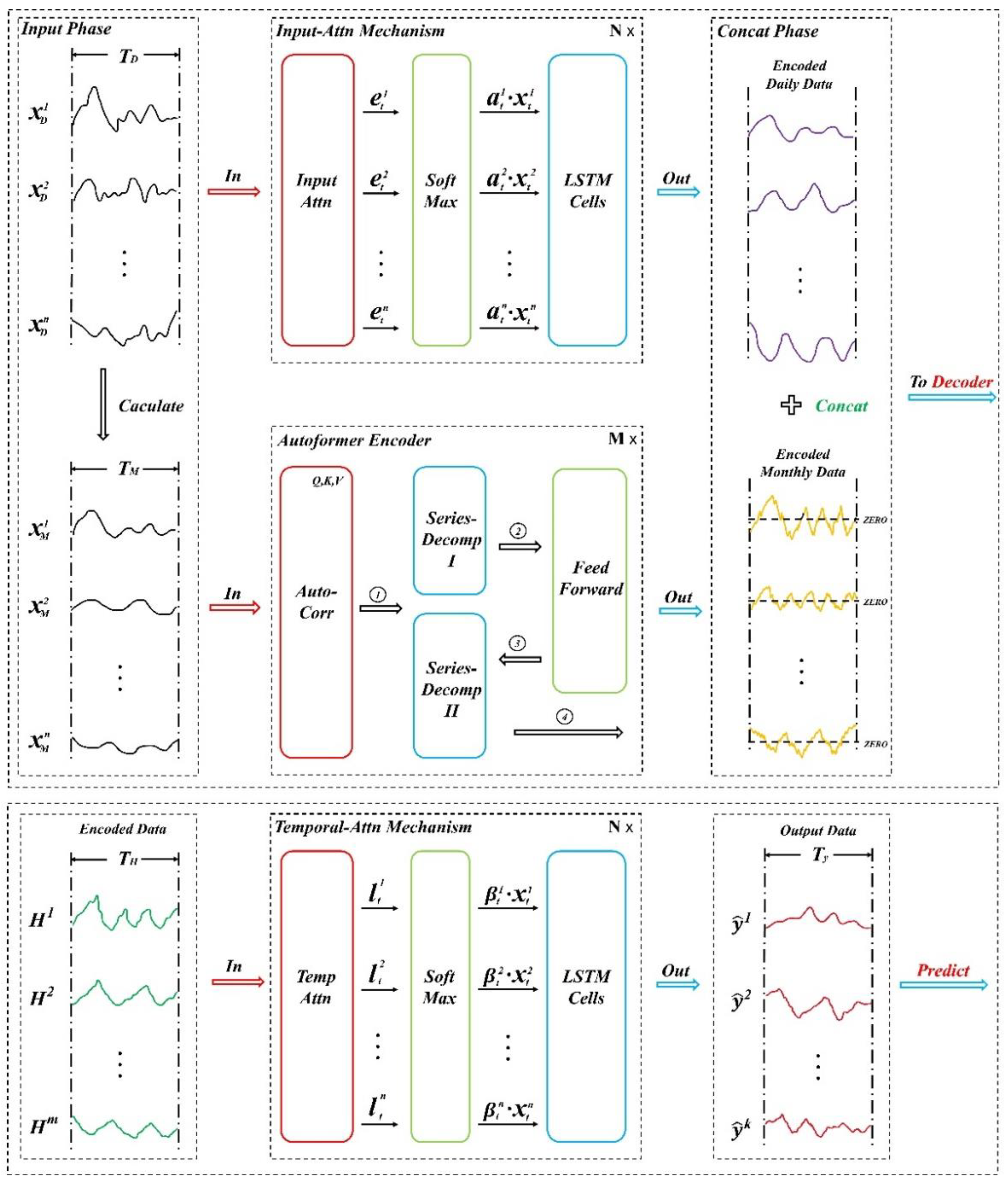
Figure 2.
Ten Steps MST-GHF Predicted Values and True Values on dataset.
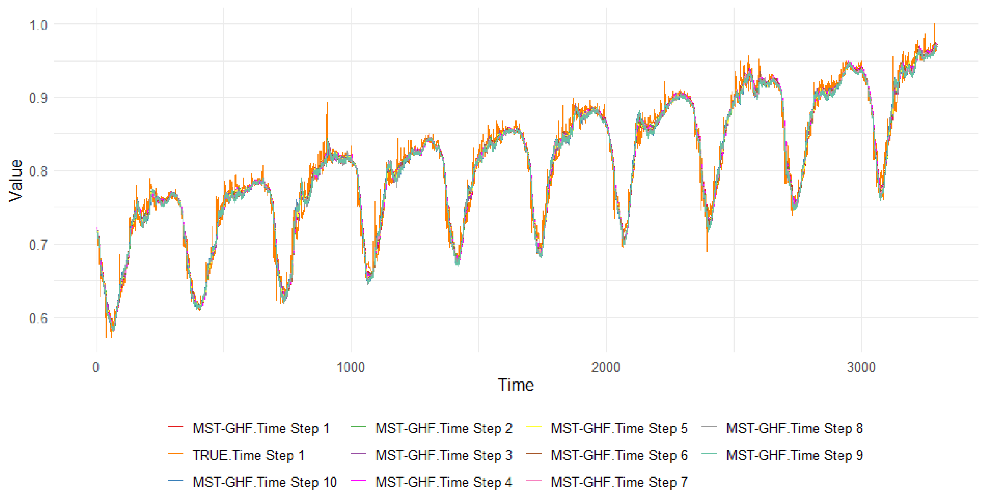
Figure 3.
The predicted values and true values of the nine best model.
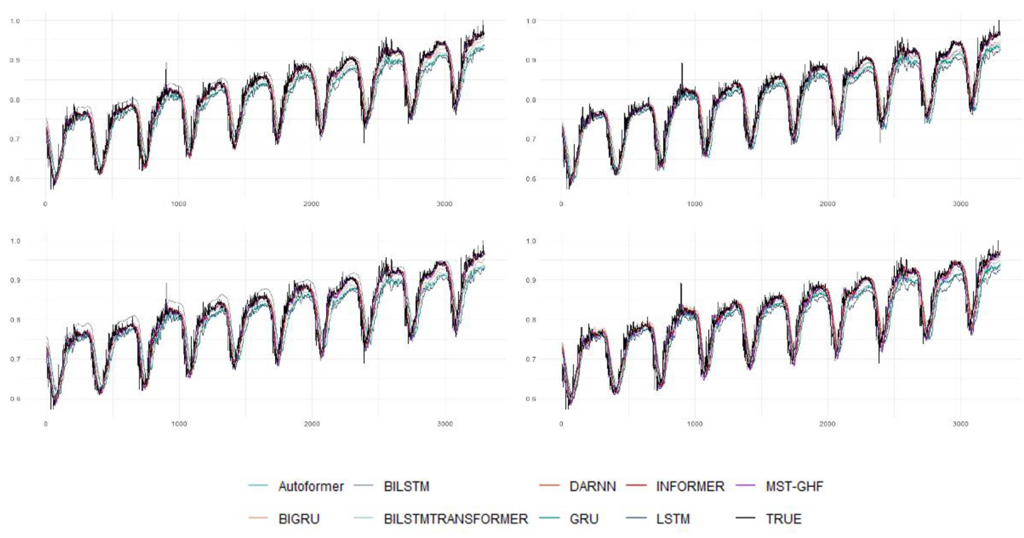

Table 1.
All test set data of 15 models.
| Model | Test_MSE | Test_MAE | Test_R² | Test_MAPE |
|---|---|---|---|---|
| MST-GHF | 0.0002878 | 0.0116377 | 0.9627339 | 0.0147310 |
| DARNN | 0.0003716 | 0.0131211 | 0.9518857 | 0.0167605 |
| Autoformer | 0.0004013 | 0.0136400 | 0.9480379 | 0.0174719 |
| TCN | 0.0004571 | 0.0146228 | 0.9408147 | 0.0187982 |
| BiTransfomer_LSTM | 0.0005962 | 0.0184426 | 0.9227868 | 0.0231243 |
| Informer | 0.0006874 | 0.0182407 | 0.9109833 | 0.0236269 |
| LSTM | 0.0008636 | 0.0243913 | 0.8881612 | 0.0295327 |
| Bi_GRU | 0.0012059 | 0.0257306 | 0.8438375 | 0.0333236 |
| Bi_LSTM | 0.0012679 | 0.0260454 | 0.8358032 | 0.0338971 |
| GRU | 0.0012723 | 0.0292467 | 0.8352157 | 0.0367302 |
| RNN | 0.0013303 | 0.0306885 | 0.8276975 | 0.0373433 |
| CNN1D | 0.0018290 | 0.0351233 | 0.7631485 | 0.0422021 |
| Bi_RNN | 0.0025301 | 0.0413129 | 0.6723005 | 0.0485256 |
| CNN1D_LSTM | 0.0028931 | 0.0447957 | 0.6253179 | 0.0527006 |
| ANN | 0.0043728 | 0.0612601 | 0.4336226 | 0.0744804 |
Table 2.
10 step Test_R² data of 15 models participating in the experiment.
| Model | STEP1 | STEP2 | STEP3 | STEP4 | STEP5 | STEP6 | STEP7 | STEP8 | STEP9 | STEP10 |
|---|---|---|---|---|---|---|---|---|---|---|
| MST-GHF | 0.97878 | 0.97443 | 0.97074 | 0.96684 | 0.96564 | 0.96125 | 0.95805 | 0.95458 | 0.95005 | 0.94698 |
| DARNN | 0.97102 | 0.96757 | 0.96023 | 0.95383 | 0.95822 | 0.94851 | 0.94829 | 0.94355 | 0.93422 | 0.93341 |
| Autoformer | 0.96930 | 0.96559 | 0.95608 | 0.94813 | 0.95578 | 0.94324 | 0.94548 | 0.93990 | 0.92843 | 0.92844 |
| TCN | 0.96514 | 0.96146 | 0.94898 | 0.93800 | 0.95049 | 0.93385 | 0.93957 | 0.93361 | 0.91780 | 0.91926 |
| BiTransfomer_LSTM | 0.94296 | 0.92876 | 0.93205 | 0.92333 | 0.91395 | 0.94672 | 0.90693 | 0.91436 | 0.91156 | 0.90723 |
| Informer | 0.94596 | 0.94410 | 0.92072 | 0.89425 | 0.92664 | 0.89500 | 0.91480 | 0.90963 | 0.87846 | 0.88027 |
| LSTM | 0.91190 | 0.90502 | 0.90029 | 0.88391 | 0.89488 | 0.90956 | 0.88113 | 0.85724 | 0.86588 | 0.87179 |
| Bi_GRU | 0.88297 | 0.83717 | 0.90740 | 0.88788 | 0.84569 | 0.76714 | 0.91339 | 0.78506 | 0.74577 | 0.86590 |
| Bi_LSTM | 0.85418 | 0.92533 | 0.88067 | 0.78546 | 0.82317 | 0.80695 | 0.76901 | 0.85771 | 0.80601 | 0.84954 |
| GRU | 0.85939 | 0.84737 | 0.86361 | 0.88095 | 0.79092 | 0.82703 | 0.83580 | 0.79108 | 0.85289 | 0.80312 |
| RNN | 0.85730 | 0.84250 | 0.84315 | 0.82455 | 0.82357 | 0.82105 | 0.80826 | 0.81793 | 0.82042 | 0.81823 |
| CNN1D | 0.79477 | 0.79974 | 0.86495 | 0.76666 | 0.71630 | 0.78686 | 0.73372 | 0.79676 | 0.71642 | 0.65530 |
| Bi_RNN | 0.72101 | 0.70851 | 0.72330 | 0.66788 | 0.61899 | 0.65601 | 0.62097 | 0.69373 | 0.66151 | 0.65108 |
| CNN1D_LSTM | 0.70959 | 0.63854 | 0.65612 | 0.62404 | 0.70758 | 0.59694 | 0.67335 | 0.53487 | 0.60110 | 0.51105 |
| ANN | 0.51734 | 0.44780 | 0.37191 | 0.43568 | 0.46613 | 0.43010 | 0.44904 | 0.45915 | 0.47785 | 0.28123 |
Table 3.
10 step Test_MSE data of 15 models participating in the experiment.
| Model | STEP1 | STEP2 | STEP3 | STEP4 | STEP5 | STEP6 | STEP7 | STEP8 | STEP9 | STEP10 |
|---|---|---|---|---|---|---|---|---|---|---|
| MST-GHF | 0.000163 | 0.000197 | 0.000226 | 0.000256 | 0.000265 | 0.000299 | 0.000324 | 0.000351 | 0.000386 | 0.000410 |
| DARNN | 0.000223 | 0.000250 | 0.000307 | 0.000356 | 0.000322 | 0.000398 | 0.000400 | 0.000436 | 0.000509 | 0.000515 |
| Autoformer | 0.000236 | 0.000265 | 0.000339 | 0.000400 | 0.000341 | 0.000438 | 0.000421 | 0.000465 | 0.000553 | 0.000554 |
| TCN | 0.000268 | 0.000297 | 0.000393 | 0.000478 | 0.000382 | 0.000511 | 0.000467 | 0.000513 | 0.000636 | 0.000625 |
| BiTransfomer_LSTM | 0.000439 | 0.000549 | 0.000524 | 0.000591 | 0.000664 | 0.000411 | 0.000719 | 0.000662 | 0.000684 | 0.000718 |
| Informer | 0.000416 | 0.000431 | 0.000611 | 0.000816 | 0.000566 | 0.000811 | 0.000658 | 0.000699 | 0.000940 | 0.000926 |
| LSTM | 0.000678 | 0.000732 | 0.000769 | 0.000896 | 0.000811 | 0.000698 | 0.000919 | 0.001104 | 0.001037 | 0.000992 |
| Bi_GRU | 0.000901 | 0.001255 | 0.000714 | 0.000865 | 0.001191 | 0.001798 | 0.000669 | 0.001662 | 0.001966 | 0.001037 |
| Bi_LSTM | 0.001123 | 0.000575 | 0.000920 | 0.001655 | 0.001365 | 0.001491 | 0.001785 | 0.001100 | 0.001500 | 0.001164 |
| GRU | 0.001083 | 0.001176 | 0.001052 | 0.000918 | 0.001614 | 0.001336 | 0.001269 | 0.001615 | 0.001138 | 0.001523 |
| RNN | 0.001099 | 0.001214 | 0.001209 | 0.001354 | 0.001362 | 0.001382 | 0.001482 | 0.001407 | 0.001389 | 0.001406 |
| CNN1D | 0.001581 | 0.001543 | 0.001041 | 0.001800 | 0.002190 | 0.001646 | 0.002058 | 0.001571 | 0.002193 | 0.002667 |
| Bi_RNN | 0.002149 | 0.002246 | 0.002133 | 0.002562 | 0.002941 | 0.002657 | 0.002929 | 0.002368 | 0.002618 | 0.002699 |
| CNN1D_LSTM | 0.002237 | 0.002785 | 0.002651 | 0.002900 | 0.002257 | 0.003113 | 0.002524 | 0.003596 | 0.003085 | 0.003783 |
| ANN | 0.003717 | 0.004255 | 0.004843 | 0.004354 | 0.004121 | 0.004401 | 0.004257 | 0.004181 | 0.004038 | 0.005561 |
Table 4.
10 step Test_MAE data of 15 models participating in the experiment.
| Model | STEP1 | STEP2 | STEP3 | STEP4 | STEP5 | STEP6 | STEP7 | STEP8 | STEP9 | STEP10 |
|---|---|---|---|---|---|---|---|---|---|---|
| MST-GHF | 0.008435 | 0.009374 | 0.010210 | 0.010994 | 0.011186 | 0.012021 | 0.012577 | 0.013206 | 0.013918 | 0.014457 |
| DARNN | 0.010061 | 0.010630 | 0.011907 | 0.012869 | 0.012302 | 0.013680 | 0.013829 | 0.014469 | 0.015657 | 0.015807 |
| Autoformer | 0.010274 | 0.010891 | 0.012558 | 0.013691 | 0.012639 | 0.014409 | 0.014199 | 0.014928 | 0.016397 | 0.016415 |
| TCN | 0.010958 | 0.011553 | 0.013643 | 0.015087 | 0.013372 | 0.015661 | 0.014940 | 0.015786 | 0.017707 | 0.017521 |
| Informer | 0.013944 | 0.014224 | 0.017385 | 0.020133 | 0.016555 | 0.020105 | 0.018042 | 0.018612 | 0.021806 | 0.021601 |
| BiTransfomer_LSTM | 0.016098 | 0.018339 | 0.017876 | 0.018638 | 0.020110 | 0.013880 | 0.020849 | 0.019472 | 0.019489 | 0.019675 |
| LSTM | 0.021328 | 0.022347 | 0.022861 | 0.024917 | 0.023618 | 0.021431 | 0.025366 | 0.028250 | 0.027284 | 0.026510 |
| Bi_GRU | 0.022423 | 0.026983 | 0.021235 | 0.022717 | 0.026333 | 0.032263 | 0.019261 | 0.030710 | 0.032259 | 0.023122 |
| Bi_LSTM | 0.024449 | 0.017924 | 0.022438 | 0.029404 | 0.027164 | 0.028833 | 0.031595 | 0.024125 | 0.027837 | 0.026685 |
| GRU | 0.027698 | 0.027475 | 0.026573 | 0.025132 | 0.033664 | 0.030206 | 0.029865 | 0.032262 | 0.028023 | 0.031569 |
| RNN | 0.027605 | 0.029178 | 0.029061 | 0.030809 | 0.031127 | 0.031362 | 0.032624 | 0.031747 | 0.031580 | 0.031791 |
| CNN1D | 0.032972 | 0.032569 | 0.026367 | 0.035236 | 0.038554 | 0.033392 | 0.037443 | 0.033172 | 0.038725 | 0.042803 |
| Bi_RNN | 0.037570 | 0.038244 | 0.037586 | 0.041467 | 0.044881 | 0.042510 | 0.044928 | 0.040119 | 0.042524 | 0.043299 |
| CNN1D_LSTM | 0.038234 | 0.043631 | 0.042643 | 0.044788 | 0.038907 | 0.046889 | 0.041832 | 0.051089 | 0.047142 | 0.052802 |
| ANN | 0.057103 | 0.060965 | 0.065537 | 0.061544 | 0.059535 | 0.061573 | 0.060271 | 0.059627 | 0.057873 | 0.068573 |
Table 5.
10 step Test_MAPE data of 15 models participating in the experiment.
| Model | STEP1 | STEP2 | STEP3 | STEP4 | STEP5 | STEP6 | STEP7 | STEP8 | STEP9 | STEP10 |
|---|---|---|---|---|---|---|---|---|---|---|
| MST-GHF | 0.010664 | 0.011856 | 0.012908 | 0.013898 | 0.014153 | 0.015210 | 0.015928 | 0.016728 | 0.017639 | 0.018326 |
| DARNN | 0.012742 | 0.013492 | 0.015195 | 0.016444 | 0.015651 | 0.017497 | 0.017647 | 0.018523 | 0.020128 | 0.020286 |
| Autoformer | 0.013061 | 0.013875 | 0.016077 | 0.017557 | 0.016118 | 0.018489 | 0.018148 | 0.019151 | 0.021127 | 0.021117 |
| TCN | 0.013990 | 0.014770 | 0.017531 | 0.019441 | 0.017128 | 0.020177 | 0.019164 | 0.020293 | 0.022875 | 0.022614 |
| BiTransfomer_LSTM | 0.019778 | 0.022580 | 0.022051 | 0.023331 | 0.025092 | 0.017770 | 0.026130 | 0.024649 | 0.024767 | 0.025097 |
| Informer | 0.017983 | 0.018345 | 0.022511 | 0.026143 | 0.021399 | 0.026094 | 0.023321 | 0.024085 | 0.028329 | 0.028060 |
| LSTM | 0.025587 | 0.026832 | 0.027559 | 0.030017 | 0.028598 | 0.026056 | 0.030931 | 0.034351 | 0.033116 | 0.032278 |
| Bi_GRU | 0.028922 | 0.034812 | 0.027270 | 0.028817 | 0.033980 | 0.042075 | 0.024814 | 0.040054 | 0.042387 | 0.030106 |
| Bi_LSTM | 0.032075 | 0.022765 | 0.029086 | 0.038758 | 0.035504 | 0.037625 | 0.041396 | 0.031411 | 0.036513 | 0.033838 |
| GRU | 0.034505 | 0.034609 | 0.033364 | 0.031164 | 0.042297 | 0.037924 | 0.037472 | 0.041016 | 0.035105 | 0.039846 |
| RNN | 0.033020 | 0.035437 | 0.035304 | 0.037536 | 0.037904 | 0.038326 | 0.039871 | 0.038640 | 0.038453 | 0.038941 |
| CNN1D | 0.039474 | 0.038810 | 0.032060 | 0.042228 | 0.046183 | 0.040666 | 0.045155 | 0.039777 | 0.046488 | 0.051180 |
| Bi_RNN | 0.043991 | 0.044804 | 0.044306 | 0.048538 | 0.052553 | 0.049851 | 0.052712 | 0.047334 | 0.050156 | 0.051010 |
| CNN1D_LSTM | 0.044628 | 0.051063 | 0.050001 | 0.052544 | 0.045748 | 0.055173 | 0.049362 | 0.060271 | 0.055763 | 0.062453 |
| ANN | 0.069636 | 0.074062 | 0.079720 | 0.074864 | 0.072489 | 0.074870 | 0.073280 | 0.072609 | 0.070289 | 0.082984 |
Disclaimer/Publisher’s Note: The statements, opinions and data contained in all publications are solely those of the individual author(s) and contributor(s) and not of MDPI and/or the editor(s). MDPI and/or the editor(s) disclaim responsibility for any injury to people or property resulting from any ideas, methods, instructions or products referred to in the content. |
© 2025 by the authors. Licensee MDPI, Basel, Switzerland. This article is an open access article distributed under the terms and conditions of the Creative Commons Attribution (CC BY) license (http://creativecommons.org/licenses/by/4.0/).
Copyright: This open access article is published under a Creative Commons CC BY 4.0 license, which permit the free download, distribution, and reuse, provided that the author and preprint are cited in any reuse.


