
Submitted:
17 February 2025
Posted:
18 February 2025
You are already at the latest version
Abstract
Inulin enzymatic hydrolysis becomes in the last years a very promising alternative to produce fructose on a large scale. Genetically modified chicory was used to extract inulin of industrial quality. By using an adequate kinetic model from literature, the present paper is aiming at determining the optimal operating alternatives of a batch (BR), or a fed-batch (FBR) reactor used for the inulin hydrolysis to fructose. Operation of FBR with a constant or a variable/dynamic feeding is compared to the BR operation to determine the most favorable option to maximize the reactor production, with minimizing the enzyme consumption. Multi-objective optimal solutions are also investigated by using the Pareto optimal fronts technique.
Keywords:
inulin hydrolysis to fructose
; batch and fedbatch reactor
; production maximization
; insilico analysis
; Pareto fronts
; FBR dynamic feeding
1. Introduction
“Biocatalytic processes produce fewer by-products, consume less energy, and generate less environmental pollution, with using smaller catalyst concentrations and much moderate reaction conditions compared to the classical chemical catalysis [1]. By displaying a high selectivity and specificity, they are sustainable bioengineering routes to obtain a wide range of products, they tend more and more to replace some of the classical fine chemical synthesis processes [2].
However, the crucial aspect in any realistic engineering analysis for process design, operation, control, and optimization relies on the knowledge of an adequate and enough reliable mathematical model of the process [3]. Such a kinetic model, preferably based on the reaction mechanism and including the key details (e.g. enzyme deactivation), has to ensure interpretable and reliable predictions of the enzymatic process behavior under various operating conditions.”[3,4,5]
In spite of their large volumes, enzymatic reactors continuously mixed tank reactors, operated in BR , or FBR modes are the most used because they ensure a high mass transfer, and a rigorous temperature/pH control.
Concerning the reactor, an essential engineering problem is referring to the development of optimal operating policies seeking for production maximization, raw-material minimum consumption, with obtaining a product of high purity. This problem depends on the i) adopted technology (chemical, biochemical, or biological catalysis), but also ii) on the used engineering analysis to optimize the reactor operation (this paper).
In the BR/FBR case, its optimal operation problem can be in-silico solved in two alternatives: (a) off-line (or ‘run-to-run’), the optimal operating policy being determined by using an adequate kinetic model previously identified based on experimental data (this paper) [6,7,8,9,10,11,12,13]; (b) on-line, by using a simplified, often empirical math model to obtain a state-parameter estimator based on the on-line recorded data (such as the classical Kalman filter) [10,14,15,16,17,18,19,20,21]. One of the in-silico , off-line analysis advantages it is that which makes it possible to compare performances of various bioreactor constructive / operating alternatives [22,23].
“Even if the enzymatic process (or bioprocess) kinetics, and the biocatalyst characteristics (inactivation rate) are known, in-silico solving this off-line engineering problem is not an easy task, due to multiple contrary objectives, and a significant degree of uncertainty of the model/constraints originating from multiple sources [14,24,25]. Due to such reasons, the reactor optimal operating policies are determined by using heuristic, stochastic, or deterministic optimization rules [11,15,23,26,27]. In the deterministic alternative (this paper), common economic objectives including the productivity, operating and (raw-)materials costs, product quality, etc., are usually used to in-silico obtain feasible optimal operating (control) policies for the analyzed reactor [25] by using specific numerical algorithms.”[12,16,21,24,28] Typical optimization objective functions were reviewed by [29,30].
“In spite of its low productivity, BRs are commonly used for slow processes (as also the case here), because they are highly flexible and easy to operate [31], in various alternatives [23]: (i).- simple BR, when substrate(s), biocatalyst, and additives are initially loaded in recommended amounts [2,22,32,33,34]. Usually, a single- or multi-objective BR optimization is off-line performed to determine the best batch time, and its initial load [14,26,32,35]; (ii).- a batch-to-batch (BR-to-BR) optimization, by including a model updating step based on acquired information from the past batches (so-called “tendency modelling”, not approached here) to determine the optimal load of the next BR [7,8,9,15,28,36,37,38,39]; (iii).- an optimally operated serial sequence of BR-s (SeqBR) [38]. The SeqBR includes a series of BRs of approx. equal volumes. At the batch end of every BR, its content is transferred to the next BR, with adjusting the reactants and/or biocatalyst(s) concentrations at optimal levels, a-priori determined to ensure the optimal SeqBR operation [9,28]. (iv).- The Semi-Batch Reactor (SBR) or fed-batch reactor (FBR), with an optimally varied feeding policy of biocatalyst/substrate(s) (not discussed here, see [22,23,24,25,32,40,41]. Usually, FBRs reported better performances compared to other batch operating alternatives. However, they are more difficult to operate, because they need previously prepared stocks of biocatalyst, and substrate(s), of different concentrations (a-priori in-silico determined), to be fed for every ‘time-arc’ of the batch (that is a batch-time division in which the feeding composition is constant; self-understood, the feeding of time-‘arcs’ usually differ between them) [22,23,24,27,42,43]. The time-step-wise variable optimal feeding policy of SBR/FBR are determined off-line [23], or on-line [20]. A comparative discussion of the all mentioned bioreactor operating alternatives is provided” by Koller [44], and Maria [23].
Fructose is a sweetener of high value in the food industry and medicine. As other polyols largely used as sweeteners (e.g. sorbitol, mannitol, xylitol, erythritol), it is produced on a large scale by using chemical, biochemical, or biological catalysis [45,46].
The chemical catalytic hydrogenation of glucose on Ni, Fe, Pt, or Fe-Ni alloy catalysts) suffers of a large numbers of disadvantages: consumes a lot of energy, occurring at high pressures (10-125 atm), and temperatures (100-140oC), while the catalyst is very expensive. Besides, the large number of by-products formed during the reaction, makes the product purification to be costly [47].
Currently, the fructose is produced by enzymatic isomerisation of glucose to fructose on Fe/CarbonBlack catalyst [46], or over some salts at 50-60oC and pH=7-8.5 [48]. This last technology starts from the high-fructose syrup (HFCS) obtained from starch [48]. Then, after rough/fine filtration, ion exchange, and evaporation, a glucose isomerization step lead obtaining a high fructose syrup (HFS, of 42-55% fructose) [48,49,50,51]. The process, intensively studied and kinetically characterized, suffers from of a series of inconvenients appropriately described in the footnote [d] of Table 1.
The biocatalytic routes to produce fructose are more convenient due to a large number of advantages: they consume less energy, by occurring at ambiental conditions, and they produce less waste due to the high yield and selectivity, the product being free of allergenic compounds. A short review of three enzymatic routes to produce fructose at industrial scale is summarized in Table 1.
Te recently developed two-steps Cetus process (Figure 1, and Table 1) leads to obtaining of a high purity fructose [52,53], as followings: Step 1) D-glucose is converted to keto-D-glucose (kDG) with a very high conversion and selectivity (more than 99%) in the presence of pyranose 2-oxidase (P2Ox) and catalase (to avoid the quick inactivation of P2Ox by the H2O2 formed in the main oxidation reaction), at 25-30oC and pH=6-7, with a very high conversion and selectivity [22,54,55]; Step 2) The kDG is then reduced to D-fructose by NAD(P)H-dependent ALR (aldose reductase, EC 1.1.1.21), at 25oC and pH=7 [56], the NAD(P)+ being in-situ or externally regenerated and re-used [57,58,59,60,61,62,63]. However, according to the results of Maria and Ene [56], the use of NADH instead of NADPH is preferable because NADPH deactivates very quickly and it is much more expensive than NADH [57].
The process drawbacks are coming from the very fast deactivation of P2Ox by one of the oxidation products (H2O2), even if the addition of catalase [22,52,64], or modification of the oxidase [65] might increase very much the enzyme half-life. The process is not yet competitive due to the costly enzymes in the both steps.
Another promising biochemical route is the enzymatic hydrolysis of inulin (Figure 2). The inulin is industrially extracted from the genetically modified chicory crops [66,67,68,69], or from modified Aspergillus sp. cultures [67,70]. The reported high conversion and selectivity of the hydrolysis process, and its simplicity recommends it as a worthy industrial alternative to produce fructose of a high quality.
In fact, “inulin is a polyfructan found in many plants as a storage carbohydrate. It contains up to 70 units of D-fructose linked to a terminal glucose, which means that inulin is a mixture of oligomers and polymers [66]. Consequently, inulin is a rich source of fructose, currently used as a macronutrient substitute or as a supplement added in foods. Being a prebiotic, industrial production of oligofructose and then of fructose from inulin is of highly interest, explaining the large number of researches in this area over the last decades [67,68,69,71]. Inulin properties, listed in Table 2, indicates a high solubility, depending on its source, from 60 g/L at 10oC, up to 400 g/L (20oC-90oC). However, the recommended concentration in manipulation is of maximum 100-200 g/L due to its tendency of precipitation and increase in the solution viscosity [70]. Water solution viscosity is close to those of water for concentrations less than 100 g/L (max. 1.0055 cP, [74]), but increase sharply for concentrated solutions [72]. Other properties of diluted inulin solutions are available in literature, being comparable to those of water (density of ca. 1.024 g/mL at 55oC [73]), and molecular diffusivity of 1.3-1.7⋅10-10 m2/s [74,75] for solutions less than 100 g/L]. The main component of inulin, that is fructose, is extremely soluble in water (ca. 22.2 M at room temperature, [76]), with diluted solution properties similar to those of water (density of up to 1.1 g/mL [77]), viscosity up to 1.2 cP [78], and a molecular diffusivity of 1.2⋅10-10 m2/s [79] for solutions less than 100 g/L]. Only the viscosity increases very sharply for concentrated fructose solutions (more than 600 cP for 70% fructose, [76]).
The fructose polymerisation degree in inulin (m) (Figure 2) depends on its origin, being of m = 27-29 in the commercially available inulin from dahlia, Jerusalem artichoke or chicory. The content of inulin in plants also vary from 1% in banana, barley, or wheat, to ca. 2-7% in globe artichoke, leek, or onion, and even to ca. 15-25% in chicory roots, dandelion, garlic, Jerusalem artichoke, and salsify. Genetically improved cultures of chicory might raise the inulin content making its industrialization attractive for production of fructose by inulin hydrolysis using inulinase (E.C. 3.2.1.7).”[67].
The purified free-inulinase activity is very high at 50-60oC and pH=4-6, but it decreases rapidly at higher temperatures (half-life of =17 min at 60oC, comparatively to =34 hrs at 50oC; [67]). Consequently, several enzyme immobilization possibilities have been searched for, some less successfully (half-life of =138 hrs at 40oC, and =7.2 hrs at 50oC in calcium alginate; [80]), but some else more promising (=21 days at 40oC, and =1.1 days at 55oC on Amberlite-support; [81]). Thermal stability of the enzyme decreases sharply with the temperature, being one of the major causes for activity decay, and running temperatures higher than 60oC are not recommended.
“As another experimental observation, enzyme immobilization decreases very much its activity. For instance, the fresh-enzyme reaction rate of 0.048 g/L.min is 4x higher than for the immobilized case (on Amberlite support). Immobilization on other supports have also been investigated, e.g. on aminoethylcellulose [82], chitin [83], amino-cellulofine beads [84], calcium alginate, agar, gelatin, cellulose [85,86], or macroporous ionic polystyrene beads [87]. In all cases the enzyme activity decreases several times after immobilization. Some metal ions, such as Hg2+ or Ag+, strongly inhibit the enzyme activity, while others (Cu2+, Fe3+) has a little or a negligible effect on the free/immobilized enzyme. Various sources of inulinase are studied, including production from recombinant bacteria [67]. Immobilized inulinase from K. fragilis on yeast cells have also been tested, reporting promising results after 30 hrs of batch runs.” [88].
By adopting an adequate kinetic model from the literature [68,69], and starting from the nominal (not-optimal) operating conditions of Table 2.[68,69,71], the in-silico analysis of this paper is aiming to evaluate and compare the performances of several optimal operating policies of a BR , and of a FBR used for the inuline hydrolysis on a free (suspended) inulinase.
Several numerical rules have been used in this respect in a novel computational methodology. Thus, the BR optimal initial load, or the time step-wise variable feeding policy with multiple control variables of a FBR are determined by using a nonlinear programming (NLP) procedure, or a Pareto optimal front technique, seeking for a single objective optimization (i.e. the fructose production maximization), or for multiple objective optimization (i.e. raw-materials consumption minimization), in the presence of various technological constraints.
2. The Experimental Enzymatic Reactor
The analyzed BR here is those used by [68,69,71] to study the inulin hydrolysis, and eventually to derive a kinetic model of this process. The characteristics of this BR are presented in Table 2, while a reduced scheme is presented by Maria et al. [97]. The reactor includes a large number of facilities, so its operation is completely automated, with a tight control of the pH, temperature, mixing speed, and feeding.
“In the BR operating mode, substrate(s), biocatalyst, and additives are only initially loaded in optimum amounts, to be in-silico determined by solving an optimization problem (product maximization here) in the presence of multiple technological constraints.
In the FBR operating mode, the substrate(s)/biocatalyst, and additives (pH-control substances, etc.) are continuously added during the batch, following a time-step-wise variable (optimal) policy, and a variable feed flow rate, to be in-silico determined by solving off-line an optimization problem (this paper, and [23,27]), or an on-line one [20]. The FBR presents a similar construction to a BR, and similar modelling hypotheses. In both cases (BR or FBR), there is no discharge (effluent) during the batch.”
3. Process Kinetics and Reactor Dynamic Model
The main reaction pathway, including the successive enzymatic hydrolysis of the inulin is presented in Figure 2. Based on the experimental data presented in (Figure 3, the blue kinetic curves), collected from a not-optimally operated BR of (Table 2) Ricca et al.[68,69] developed a kinetic model of this enzymatic process. This model, presented in (Table 3) is able to fairly simulate the dynamics of the process key-species [abbreviated S, F, W, G, E] over a long batch (780 min.).
“The presence of large amounts of fructose (S) inhibits the reaction, but this inhibitory effect is negligible for inulin initial concentrations less than 60 g/L [68]. The differential mass balance of species has been formulated by adopting an average fructose polymerisation degree in inulin of m= 29. An exhaustive investigation of the optimal conditions of the process was done by Rocha et al. [71], by using a commercial inulinase from Aspergillus niger. The results indicated the temperature of 50-60oC and pH=4.5 for the free-enzyme case, and 50oC and pH=5.5 for immobilized-enzyme on Amberlite, using 1-200 g/L (or higher) inulin initial concentration, as being the best choice. The time to obtain the same conversion is dependent on the temperature, and on the enzyme initial concentration, as long as its deactivation is quite significant.” [69]
To model the dynamics of the key-species in the BR/ FBR case, a classical simple common model was adopted, of ideal type [98], developed with the following main hypotheses:(i) Isothermal, iso-pH; (ii) The liquid phase is perfectly mixed (with no concentration gradients), by using a continuous mechanical mixing. (iii) The liquid volume is quasi-constant for the BR case (its increase due to the pH controlling additives being negligible). On the contrary, in the FBR case, the liquid volume, and the water (W) amount grow continuously, according to the feed flow rate adopted optimal feeding policy. (iv) There is a negligible mass resistance for the transport of compounds in the liquid phase.
In brief, the enzymatic BR model is presented in Table 4-BR, with including the mass balances of the key-species of the process, that is (Table 3): [S, F, W, G, E], all of them being observable, with a measurable concentration.
The overall hydrolysis reaction of Table 3 is of a Michaelis-Menten type, with the rate constants depending on the temperature following the classic Arrhenius law. More details about this reaction mechanism are given by Ricca et al. [68,69]. To estimate the rate constants of Table 3, by using the experimental kinetic curves of (Figure 3, blue curves), a combined Lineweaver-Burk plots, with a NLP numerical rule were applied. More details on the used estimation procedure, and on the estimated rate constants statistical quality are given by Ricca et al. [68,69].
According to the Ricca et al. [68,69], a 780 min batch time is enough to obtain a high S-conversion (96%) for the nominal (not-optimal) conditions of [S]o = 40 g/L, [E]o = 97 U/L, [W]o = 988 g/L (that is 1 L), 50oC, pH = 5. A wider range of the operating conditions has also been investigated. Consequently, the feasible ranges of the reactor control variables were set at the values specified in (Table 2).

Table 3.
Inulin hydrolysis reaction mechanism, and the reduced kinetic model proposed by Ricca et al. [68,69]. The used commercial inulinase was obtained from Aspergillus ficuum. “Notations: S = inulin (substrate); F = fructose; W = water; G = glucose; E = enzyme; Im = inulin with m-degree of fructose polymerisation; T = temperature (K); M = molecular mass (g/mol); index: S = substrate; E = enzyme; W = water; F =fructose; G = glucose.”.
| Reaction pathway (Figure 2): | |
|
; ; ; ; The above consecutive scheme is approximated by the overall reaction: | |
| Rate expressions: [a] | Parameters: |
|
; = ; = ; Or, equivalently, one can write: ; = ; = |
“m= 29; = 18 g/mol == 180 g/mol =, g/U·min [b] =, g/L ” |
| Enzyme deactivation model: | |
| - adopted first-order model: , ⇒ Or, equivalently, one can write: |
=, 1/h (experimental, free enzyme) |
| - other data from literature: “free-enzyme (Santos et al., 2007) immobilized-enzyme (Santos et al., 2007) |
, 1/min , 1/min |
| - other rate expressions (pseudo second-order, not tested here): , ⇒ free-enzyme (Catana et al., 2007) immobilized-enzyme (Catana et al., 2007)” |
, 1/h , 1/h |
Table 4.
BR. Key-species mass balances in the BR model, by including the enzymatic process kinetic model together with the associated rate constants of (Table 3). The ideal model hypotheses of [Maria, 2020B], of [Moser, 1988], and of [Dutta, 2008] assume a homogeneous liquid composition, with negligible mass transport resistance in the bulk phase.
| Species | Remarks |
|
Species mass balances: ; “j” = species index (S, F, W, G, E), With the initial conditions of: ; where “j” = (S, E, W) are to be optimized; = 0 , for j = (F, G). |
The species reaction rate () expressions, the rate constants, and the stoichiometry (νij) are given in Table 3. Enzyme (E) deactivation is included in this dynamic balance. The optimal BR initial load (Table 5) is off-line determined by in-silico solving the associated NLP optimization problem (this paper). C = species concentration vector ; k = rate constants vector |
Table 4.
FBR. Key-species mass balances in the fed-batch bioreactor FBR model, by including the enzymatic process kinetic model together with the associated rate constants of (Table 3). The ideal model hypotheses of Maria et al. [2022] assume a homogeneous liquid composition, by neglecting the mass transport resistance in the bulk phase. The time step-wise variable feeding is made over Ndiv time “arcs” (adopted Ndiv = 5 here), where Ndiv = number of equal time “arcs”, in which the batch time (tf) is divided. The control variables are ; ; , with j = 1,… Ndiv.
| Species | Remarks | |
|
Species mass balances: ; ; for species i = S, F, G, E , for i= S,E ; = control variables, where i = S,E; j = 1,.., time stepwise unknown values to be determined from the FBR optimization; For species W the mass balance is [b]: [W]o = 988 g/L; = 0 , for j = (F, G). |
For the optimal FBR with adopted Ndiv = 5, the feeding policy are (Footnote [a]): |
|
|
Liquid volume in the reactor (footnote [c]): = control variable; j = 1,..,time stepwise unknown values to be determined from the FBR optimization. The unknown = (t = 0) = is determined together with the all values. |
For the optimal FBR with adopted Ndiv =10, the feeding policy is (Footnote [a]): |
|
| ) to ensure the FBR optimal operation. | ||
4. Optimization Problem for the BR and FBR Reactors
4.1. Control Variables Selection
By analyzing the BR and FBR dynamic models of Table 4-BR and Table 4-FBR respectively, the chosen control variables are those related to the reactor initial load or its variable feeding, that is:
BR case: initial load of [S]o [E]o, [W]o (substrate, enzyme, and water respectively);
FBR case: the feed characteristics for every time-division (“arc”), that is ; ; , with j = 1,… Ndiv (number of equal time “arcs” in which the batch time is divided).
4.2. NLP Optimization with a Single Objective Function (Ω)
Optimization of a BR operation translates in finding its initial load with the key-species mentioned in section 4.1 (that is 3 unknowns in the present case), by using a common nonlinear programming (NLP) optimization rule, seeking to determine the extreme of an objective function in the presence of multiple constraints. In the present case, this problem refers to the maximization of the [F] (fructose) production, that is:
|
Given [F]o = 0, [G]o = 0, find control variables [S]o [E]o, [W]o, such that: Max Ω(C, Co, k) , where: Ω = [F(t)] |
(1-BR) |
For the FBR case, the batch time is divided in Ndiv equal “time-arcs” (adopted Ndiv = 5 here). The control variables, ; ; , with j = 1,… Ndiv, are kept constant over every “time-arc” at optimal values to be determined by solving the optimization problem Eq.(1-FBR). Self-understood, the control variables may differ between different “time-arcs”. “The time-intervals of equal lengths Δt = tf /Ndiv are obtained by dividing the batch time tf into Ndiv parts tj-1 ≤ t ≤ tj , where tj = j·Δt are switching points (where the reactor input is continuous and differentiable).”[20,22,23,27,33,42,97,99] In the present case, the switching points are presented explicitly in the Table 4-FBR.
|
Given [F]o = 0, [G]o = 0, Find the control variables: ; ; , For j = 1,…, Ndiv , with the adopted Ndiv = 5 time-arcs, and the FBR initial condition of Table 4-FBR, so as to obtain: Max Ω(C, Co, k) , where: Ω = [F(t)] |
(1-FBR) |
The optimal FBR principle is to obtain an optimal feeding policy consisting in a time stepwise variation of the control variables (i.e. feeding liquid flow rate, and the concentrations of the added substrates and biocatalyst) over the adopted Ndiv = 5 equal ‘time-arcs’ of the batch [23,99]. This implies to divide the batch time in Ndiv equal time-‘arcs’, the feeding being constant over each time-arc, but at different values between them. The suitable choice of a small Ndiv is discussed by Maria [23].
“In Eq.(1-BR), and Eq.(1-FBR), the time-varying [F(t)] is in fact a multi-variable function F(C(t),Co,k)(t), evaluated by using the process/reactor model of Table 4-BR and of Table 4-FBR respectively, over the whole batch time (t) ∈ [0, tf ]. As an observation, the (Figure 3, Figure 4A and Figure 5A) reveals that, in the present case study, the maximum [F] is reached at the batch end. Notations: C = species concentration vector; Co = initial value of C; k = kinetic model rate constants vector.
As an observation, other optimization objectives can be applied as well, for instance a multi-objective one [24]. However, the adopted single objective optimization, seeking for the main goal, presents the advantage of simplicity, an easy application and interpretation.
The [F(t)] time-evolution is determined by solving the reactor dynamic model of Table 4-BR , or Table 4-FBR over the whole batch time (t) ∈ [0, tf ], with the initial condition of Cj,0 = Cj(t=0) searched during optimization iterative numerical rule. The dynamic model solution was obtained with enough precision, by using the low-order stiff integrator (“ode15s”) of the MATLAB computational package.”
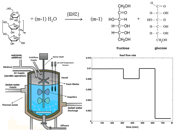
Figure 3.
[Left] Dynamics of S-conversion, and of the enzyme relative activity. [Right] Dynamics of the process key-species in the experimental not-optimally operated BR of Ricca et al.[69](1 – blue lines), compared to the optimally NLP operated BR (2 – simulated black lines). Search ranges for the control variables are given in Table 2 and Table 5.
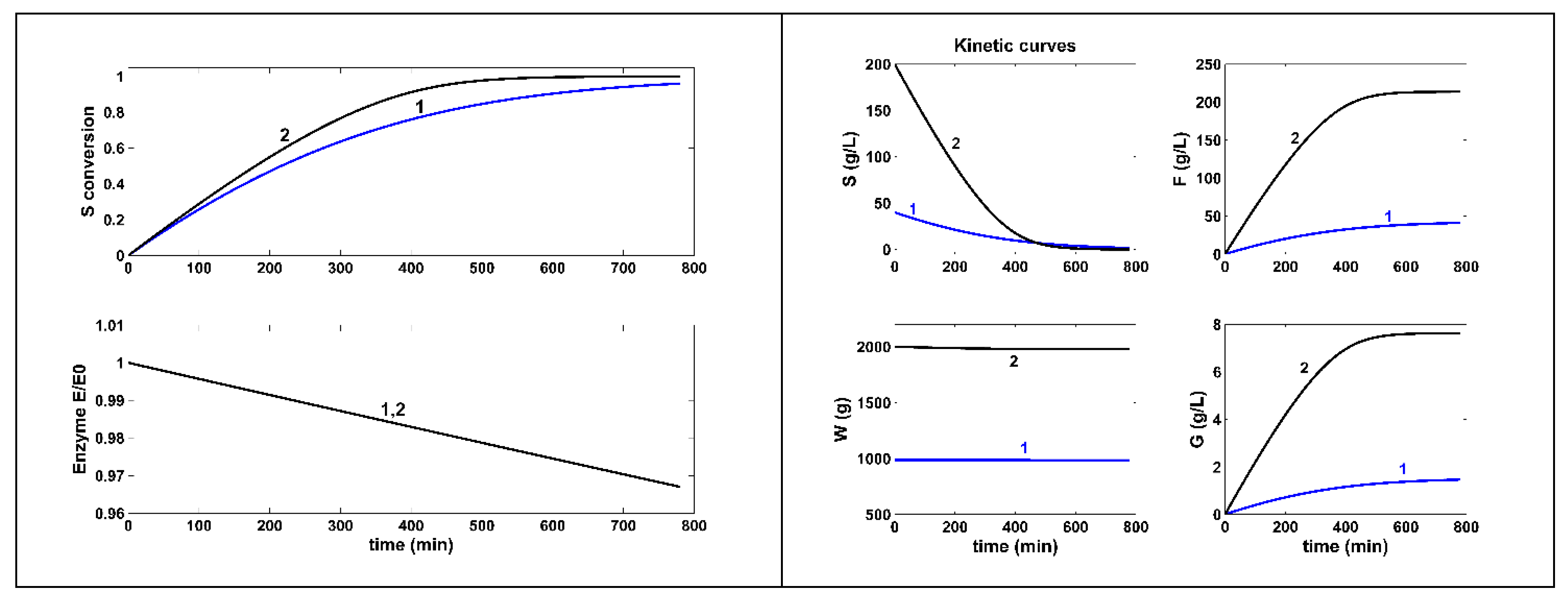
Figure 4.
[Figure [A]] Simulated species concentration dynamics for the FBR reactor with a constant but NLP optimal feeding. [Figure [B]] The optimal constant feeding with enzyme [E]in, substrate [S]in, and feed flow rate FL,in. [Figure [C]]. Enzyme dynamics in the reactor bulk, and the liquid volume increase. The control variables search ranges are given in Table 2 and Table 5. The optimal constant feeding are: [E]in = 5485.2 U/L, substrate [S]in = 400 g/L, and feed flow rate FL,in = 5.13e-4 L/min.
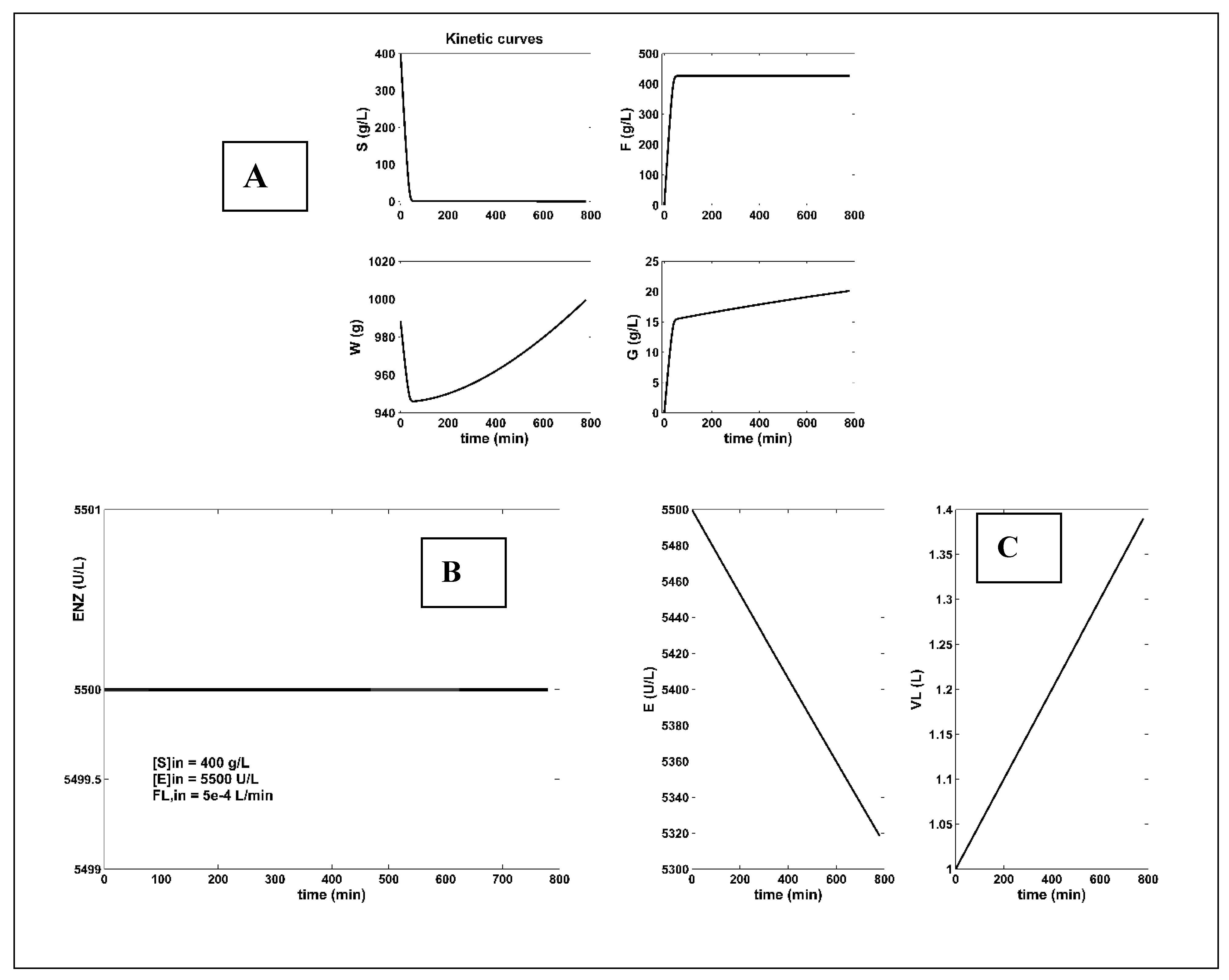
Figure 5.
[Figure [A]] Simulated species concentration dynamics for the FBR reactor with a variable but NLP optimal feeding. [Figure [B]] Enzyme dynamics in the reactor bulk, and the liquid volume increase. [Figure [C]] The optimal variable feeding with feed flow rate FL,in. [Figure [D]] The optimal step-wise variable feeding with enzyme [E]in. [Figure [E]] The optimal step-wise variable feeding with substrate [S]in. The control variables (FL,in; [S]in; [E]in) search ranges are given in Table 5.
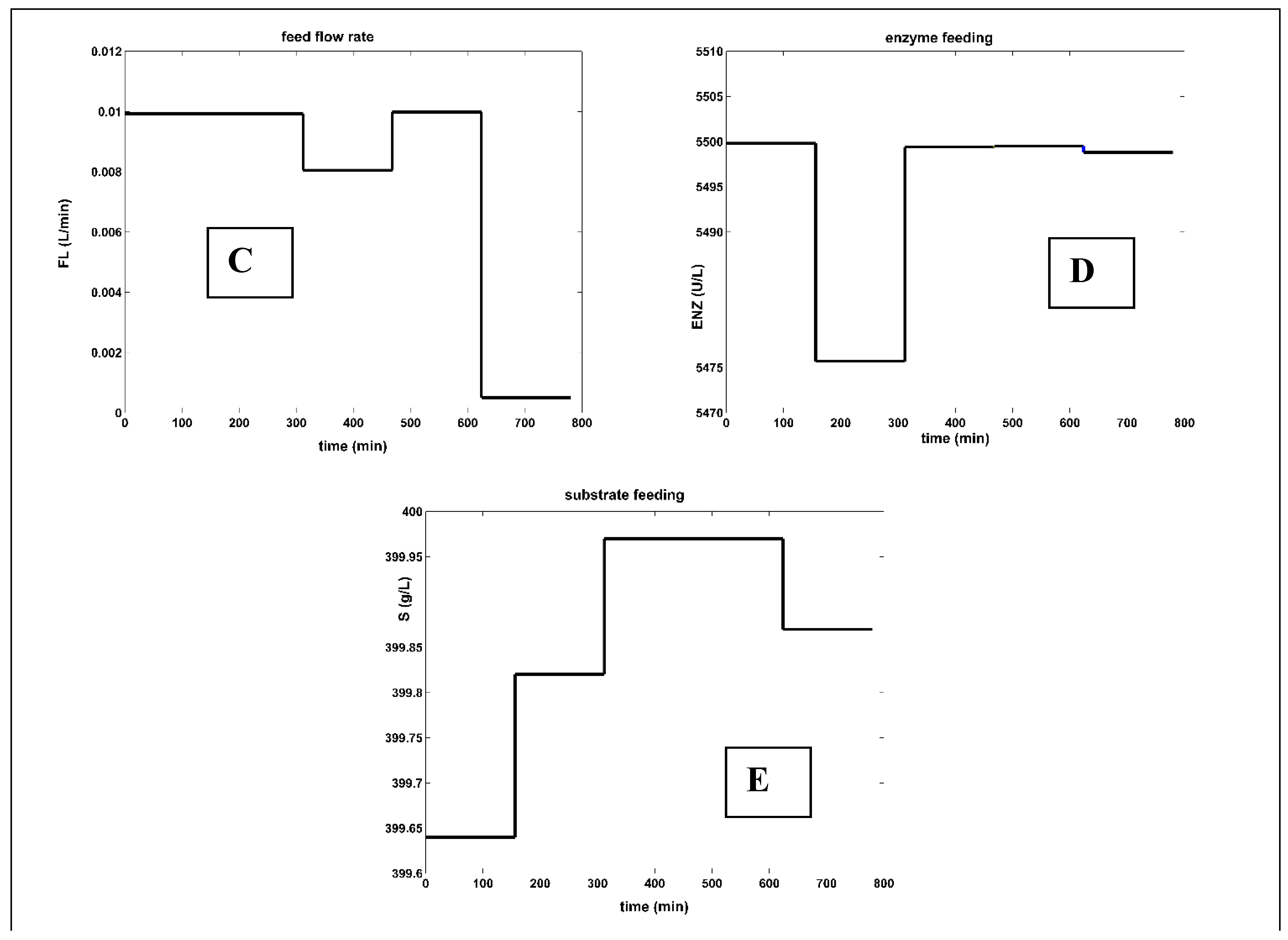
Table 5.
Efficiency of BR/FBR (Table 2) operated in various alternatives, for the inulin enzymatic hydrolysis to fructose, by using a batch time of 780 min. for all cases. A total conversion is realized in all the cases.
Table 5.
Efficiency of BR/FBR (Table 2) operated in various alternatives, for the inulin enzymatic hydrolysis to fructose, by using a batch time of 780 min. for all cases. A total conversion is realized in all the cases.
| Reactor operation | Raw-material consumption [b] |
Max F (fructose), (g)[b] |
Final VL (L) | |||||||
| Type | Ndiv | Operating parameters |
S (inulin), (g) (Eq.4) |
E (enzyme) (U) (Eq.4) |
[a] | |||||
|
BR not-optimal [Ricca et al. 2009b] |
1 |
Nominal load [c,f] (Figure 4) |
40 |
9.7 (poor) |
41.05 | 1 | ||||
| [S]o | 40 | |||||||||
| [E]o | 9.7 | |||||||||
| Wo | 988.4 | |||||||||
|
BR Optimal load NLP (this paper) [h] |
1 |
Initial load [f,b,h] (Figure 3) |
200 |
302 (fairy good) |
213.7 | 2 [g] | ||||
| [S]o | 200 | |||||||||
| [E]o | 301.87 | |||||||||
| Wo | 2000 | |||||||||
|
FBR Constant, but NLP optimal feeding, (this paper) [d] |
1 |
optimal feeding [f,j] (Figure 4) |
156 |
2145.9 (almost best) |
426.9 | 1.4 | ||||
| [S]in | 400 | |||||||||
| [E]in | 5500 | |||||||||
| FL,in | 5e-4 | |||||||||
|
FBR Constant, but Pareto optimal feeding, (this paper) [d] |
1 | optimal feeding [f,j] | 180.4 |
357.9 (best) |
422.9 | 1.4 | ||||
| [S]in | 399.88 | |||||||||
| [E]in | 793.19 | |||||||||
| FL,in | 5.78e-4 | |||||||||
|
FBR Variable optimal NLP feeding , (this paper) [e] |
5 |
optimal feeding [f,j] (Figure 5) |
2,393.7 |
3.29E+4 (high consumptions, and dilution) |
428 | 6.98 | ||||
|
[S]in [40-400] |
variable Figure 6D |
|||||||||
|
[E]in [97-5500] |
variable Figure 6D |
|||||||||
|
FL,in [5e-4 – 0.01] |
variable Figure 6C |
|||||||||
|
Footnotes: [a] Initial liquid volume VL,o = 1 L. [b] The displayed digits come from the numerical simulations. [c] The checked BR set-point of Ricca et al. [69]. [d] The FBR operation with a constant over time feeding for all the control variables, that is (Table 4-FBR): ; ; the only 3 variables to be optimized being the initial inlet values of , , , under the constraints Eq.(2i-iv). See the resulted FBR optimal operating policy in Figure 4. [e]. The FBR optimal time step-wise variable feeding policy is obtained by using the control variable limits of the footnote [j]. In this FBR operating case, the control variables, that is , , ; j = 1,…(Ndiv -1) of Table 4-FBR, follows an uneven policy to be optimized (that is 15 unknowns for Ndiv = 5). The optimal control variables policy is given in Figure 5. [f] The units are: [S] g/L ; [E] U/L ; [W] g; FL L/min. [g] The volume corresponds to the water (W) mass required by the reaction. [h] Search intervals of the control variables are the followings: [S]in = [40-200] g/L ; [E]in = [97-5500] U/L. [j] Search intervals of control variables are: [S]in = [40-400] g/L ; [E]in = [97-5500] U/L; FL,in = [5e-4 – 0.01] L/min. [67]. | ||||||||||
4.3. Optimization Problem Constraints
The above formulated nonlinear optimization problem (NLP) Eq.(1-BR), or Eq.(1-FBR), must account for the followings constraints:
(a).- The BR model of Table 4-BR, including the process kinetic model (Table 3);
(b).- The FBR model of Table 4-FBR, including the process kinetic model (Table 3);
(c).- To limit the excessive consumption of raw-materials, feasible searching ranges are imposed to the control/decision variable, as stipulated in (Table 2).
To be considered in the optimization problem Eq.(1-BR), or Eq.(1-FBR), these constraints should be ‘translated’ in a mathematical form. Eventually, the resulted NLP optimization problem is highly non-convex and nonlinear, being subjected to the following technological/physical meaning/model constraints:
|
Nonlinear process and reactor model: Table 4-BR, for the BR case. Table 4-FBR, for the FBR case. |
(2i) |
|
Physical significance constraints: “, in Table 4-BR, and Table 4-FBR, for all the species of index ‘j’, and for all t Є [0-tf]” |
(2ii) |
|
Searching ranges for the control variables are given in (Table 2), that is: [S]o; [S]in ∈ [40-400] g/L [E]o; [E]in ∈ [97-5500] (U/L) [W]o ∈ [988- 4000](g) FL ∈ [5e-4 – 0.01] (L/min) |
(2iii) |
| ≤ 10 L (reactor capacity) | (2iv) |
4.4. Pareto Optimal Front Optimization with Opposite Objective Functions
When multiple opposite objective functions are formulated for an optimization problem, an elegant alternative is to use the Pareto optimal front technique. Each Pareto optimal front (curve) accounts for two opposite optimization objectives.
Following the Pareto-front definition [100], any running point from the Pareto-curve can be a valid solution of the optimization problem. The Pareto-curve being a continuous one, “when two opposite optimization criteria are used, infinity of Pareto-optimal operating solutions can exist”. Consequently, the chosen solution (that is the FBR optimal operation set points here) is subjective and case-dependent, and it should be chosen by adding a criterion not accounted when the Pareto-front was generated. It is to note that many Pareto-fronts of different shapes can exist for the same optimization problem [24].
In the present case study, by analyzing the FBR model of Eq.(4-FBR), and its control variables, at least three Pareto fronts can be found, for the case of a constant optimal feeding, as presented by the Eq.(3). Additional objectives can exist, but the present analysis was limited to the following ones.
| Maximum F production vs.- Minimum substrate (S) consumption. Minimum constant feed flow rate, for various maximum F produced. Maximum F production vs.- Minimum enzyme (E) consumption. |
(3) |
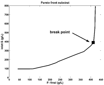
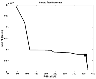
As the literature reveals [100] a lot of Pareto optimal fronts are monotonous and of an exponentially-/logarithmic-like shape. Extended studies of [42,59,105-108] for such kind of shapes, made on various (bio)chemical reacting systems, indicated that the ‘break-point’ of the Pareto-front (Figure 6, and Figure 7 in the present case) is a good choice for the optimization problem with at least two opposite objectives. As recommended, this ‘break-point’ should be with ca. 5% higher on the ordinate than the ‘base-line’ of the Pareto-curve. That is because a running point on the baseline (at the left of the ‘break-point’ in Figure 6) is not economic, by reporting a lower production of the target product; on the contrary, a running point chosen at the right of the ‘break-point’ reports a higher productivity, but with the cost of an increasingly higher enzymes consumption, and violation of the technological constraints Eq.(2). In the present case, the chosen ‘break-point’ of (Figure 6, and Figure 7) is those presented in (Table 5) and reports better performances compared to other FBR operating alternatives.
 |
 |
|
Figure 6. The Pareto-optimal front for the FBR (of Table 1) with a constant feeding in terms of two opposite objectives, that is maximum F production vs.- minimum substrate (S) consumption. This problem Eq. (3) solution was obtained by imposing the control variable limits given in Table 5. The set-point was chosen as being the “break point” of the Pareto-optimal front, according to the suggestions of Dan and Maria [42] |
Figure 7. The Pareto-optimal operating policy of the FBR (of Table 1) in terms of required minimum constant feed flow rate, for various maximum F produced. The marked point is the chosen set-point corresponding to those of the Pareto-optimal curve of Figure 6. |
4.5. The Used Solvers
During BR/FBR optimization, when simulating the reactor dynamics in every solver iteration, the model species bulk-phase concentrations are obtained by solving the dynamic model of the reactor (Table 4-BR , or Table 4-FBR, respectively)with the initial condition (t=0) being the iterative guess tried by the numerical solver. The imposed batch time , and the medium conditions are those of (Table 1). The dynamic model solution was obtained with a high precision, by using the variable-order stiff integrator (‘ode15s’) of the MATLAB package.
Because the reactor differential models, and the optimization objective Eq.(1-BR), Eq.(1-FBR), and the problem constraints eqn.(2i-iv) are all highly nonlinear, the Pareto-optimal fronts were obtained by using a multi-modal search algorithm, that is the (‘gamultiobj’) of the MATLAB package. This numerical algorithm is suitable for this non-convex and nonlinear case. “The computational time was reasonably short (minutes) using a common PC, thus offering a quick implementation of the off-line obtained BR optimal operating policy.
Because the enzymatic reactor/process kinetic model (Tables 4-BR, 4-FBR), the optimization objectives Eq.(1-BR), Eq. (1-FBR), and the problem constraints Eq.(3i-3v) are all highly nonlinear, the formulated problem Eq.(1-BR), and Eq.(1-FBR) translate into a nonlinear optimization problem (NLP) with a multimodal objective function and a non-convex searching domain. To obtain the global feasible solution with enough precision, the multi-modal optimization solver MMA of Maria [4,101,102] has been used, started from different initial guesses, as being proved to be very effective compared to the common (commercial) optimization algorithms.”
5. Optimization Results and Their Discussion
The results for solving the NLP optimization problem, are presented in the following forms:
a)-.- In (Figure 3) are displayed the NLP optimal operating policy for the analyzed BR, by comparison with the experimental data of Ricca et al. [69] obtained in a BR operated under not-optimal conditions of (Table 2).
b)-.- A comparison of all BR operating alternatives in terms of fructose (F) production and raw-materials consumption in Table 5. In the BR case, the raw-materials consumption is based on the only initial load. In the FBR case, the raw-materials consumption (mass) is computed with the following formula:
c)-.- The optimally operated FBR , with a constant but NLP optimal feeding in (Figure 4).
d)-.- The optimally operated FBR with a variable but NLP optimal feeding in (Figure 5).
By analyzing these results and, in particular, the operating alternatives of Table 5, several conclusions can be derived, as followings:
(1).- The NLP optimally operated BR , according to Eq.(1-BR), under the constraints Eq.(2i-iv) for the control variables, reported incomparably better performances (5x in terms of more produced F, by the expense of consuming 5x more substrate, and 30x more enzyme) compared to the experimental not-optial BR trial of Ricca et al.[69] (in Table 5, and in Figure 3).
(2).- By far, the best alternative is the FBR operated with a constant, but NLP optimal feeding Eq.(1-BR), or operated with using the set-point (“break point”) given by the Pareto optimal front, Eq.(3) . Even if the F-production is similar to those of the NLP optimally operated BR, the substrate consumption is 13x-15x less, by consuming 15x-92x less enzyme (Table 5 and Figure 4). As revealed by the results of Table 5, the FBR operated with a constant, but using the set-point (“break point”) given by the Pareto optimal front, Eq.(3), under the constraints Eq.(2i-iv) for the control variables, reported the best performances, regarding all the objectives mentioned above.
(3).- By analyzing the FBR with a NLP optimal variable feeding, the results are quite modest. In spite of a realized good F-production, compared to the FBR operated with a constant but Pareto optimal feeding, the FBR with an optimal NLP variable feeding reported higher raw-materials consumptions (90x more enzyme, and 13x more substrate).
(4).- Of course, enzyme stabilization by immobilization is expected to improve the process performances, as reviewed in the Introduction section [104].
(5).- The FBR optimal control strategy is very adaptable. That is because the employed process kinetic model of moderate complexity is enough flexible, due to a fairly large number of rate constants. Thus, if significant inconsistencies are observed between the model-predicted bioreactor dynamics and the recorded data, then an intermediate numerical-analysis step will be applied to improve the model adequacy (i.e. a ‘model updating’ step), and the bioreactor optimization is applied again with the novel model. This evolutionary adaptation of the enzymatic process model is the so-called ‘tendency modelling’ [39].
6. Conclusions
To conclude, the in-silico, off-line optimized BR operation, or a FBR with a constant but optimal feeding, even though there are simple alternatives to implement, they can offer a significantly improved reactor effectiveness, due to its high flexibility in using an easily adaptable process model, and due to the applied effective optimization rules (single objective NLP).
The nominal, not-optimal BR operation used to derive the process kinetic model reported very poor performances. Thus, the same BR, but NLP optimally operated by also taking into account the technological constraints for the control variables reported incomparably better performances (5x in terms of more produced fructose, by the expense of consuming 5x more substrate, and 30x more enzyme).
Our in-silico analysis reveals that the best alternative is the FBR operated with a constant, but using the set-point (“break point”) given by the Pareto optimal front of Figure 7., under the constraints Eq.(2i-iv) for the control variables. This set point reported the best performances, regarding all the objectives considered in Eq.(3).
“The present optimization analysis proves its worth by including multiple elements of novelty, as follows: i) An optimally operated FBR, by using wider but feasible ranges for setting the control variables can lead to high performances of the bioreactor. ii) The major role played by the biocatalyst (enzyme concentration) as a control variable during FBR optimization (an option seldom discussed in the literature). iii) The in-silico (model-based) optimal operation of enzymatic reactors is a very important engineering issue because it can lead to consistent economic benefits, as proved by the results presented in this paper.”
Abbreviations and Notations
| - | species j concentration | |
| ,, | - | kinetic model constants |
| k | - | rate constants vector |
| - | molecular weight | |
| - | mass | |
| - | fructose degree of polymerization in the inulin | |
| - | Number of time “arcs”, that is the number of equal divisions of the batch time for a FBR with variable feeding case | |
| - | species j reaction rate | |
| - | temperature | |
| - | time | |
| - | time interval | |
| - | batch time | |
| VL, VL | - | liquid volume |
| Greeks | ||
| ,, , , | - | Kinetic model constants |
| - | finite difference | |
| νij | - | The stoichiometric coefficient of the species “j” in the reaction “i” |
| Ω | - | optimization objective function |
| - | density | |
| Index | ||
| In, inlet | - | inlet |
| 0,o | - | initial |
| S ,F, W, E, G | - | Substrate, fructose, water, enzyme, glucose, respectivelly |
| kDG | - | Keto D-Glucose (D-glucosone) |
| Max | - | maximum |
| NLP | - | nonlinear programming |
| PO2x | - | Pyranose 2-oxidase |
| S | - | Substrate (inulin) |
| SBR | - | semi-batch reactor |
| W | - | water |
References
- Moulijn, J.A.; Makkee, M.; van Diepen, A. , Chemical process technology, Wiley, New York, 2001.
- Wang, P. Multi-scale Features in Recent Development of Enzymic Biocatalyst Systems. Appl. Biochem. Biotechnol. 2008, 152, 343–352. [Google Scholar] [CrossRef]
- Vasić-Rački, D.; Findrik, Z.; Presečki, A.V. Modelling as a tool of enzyme reaction engineering for enzyme reactor development. Appl. Microbiol. Biotechnol. 2011, 91, 845–856. [Google Scholar] [CrossRef] [PubMed]
- Maria, G. , A review of algorithms and trends in kinetic model identification for chemical and biochemical systems, Chem. Biochem. Eng. Q., 2004, 18, 195–222. [Google Scholar]
- Gernaey, K.V.; Lantz, A.E.; Tufvesson, P.; Woodley, J.M.; Sin, G. Application of mechanistic models to fermentation and biocatalysis for next-generation processes. Trends Biotechnol. 2010, 28, 346–354. [Google Scholar] [CrossRef] [PubMed]
- Bonvin, D.; Srinivasan, B.; Hunkeler, D. , Control and optimization of batch processes, IEEE Control systems magazine, 2006, 34-45.
- Srinivasan, B.; Primus, C.; Bonvin, D.; Ricker, N. Run-to-run optimization via control of generalized constraints. Control. Eng. Pr. 2001, 9, 911–919. [Google Scholar] [CrossRef]
- Dewasme, L.; Amribt, Z.; Santos, L.; Hantson, A.-L.; Bogaerts, P.; Wouwer, A.V. Hybridoma cell culture optimization using nonlinear model predictive control. IFAC Proc. Vol. 2013, 46, 60–65. [Google Scholar] [CrossRef]
- Dewasme, L.; Côte, F.; Filee, P.; Hantson, A.-L.; Wouwer, A.V. Macroscopic Dynamic Modeling of Sequential Batch Cultures of Hybridoma Cells: An Experimental Validation. Bioengineering 2017, 4, 17. [Google Scholar] [CrossRef]
- Mendes, R.; Rocha, I.; Pinto, J.P.; Ferreira, E.C.; Rocha, M. , Differential evolution for the offline and online optimization of fed-batch fermentation processes. In: Chakraborty, U.K. (ed.), Advances in differential evolution. Studies in Computational Intelligence, Springer verlag, Berlin, 2008, pp. 299-317.
- Liu, Y.; Gunawan, R. Bioprocess optimization under uncertainty using ensemble modeling. J. Biotechnol. 2017, 244, 34–44. [Google Scholar] [CrossRef]
- Hartig, F.; Keil, F.J.; Luus, R. , Comparison of optimization methods for a fed-batch reactor, Hung. J. Ind. Chem., 1996, 23, 81–160. [Google Scholar]
- Amribt, Z.; Dewasme, L.; Wouwer, A.V.; Bogaerts, P. Optimization and robustness analysis of hybridoma cell fed-batch cultures using the overflow metabolism model. Bioprocess Biosyst. Eng. 2014, 37, 1637–1652. [Google Scholar] [CrossRef]
- Bonvin, D. Optimal operation of batch reactors—a personal view. J. Process. Control. 1998, 8, 355–368. [Google Scholar] [CrossRef]
- Bonvin, D. , Real-time optimization, MDPI, Basel, 2017.
- DiBiasio, D. , Introduction to the control of biological reactors. In: Shuler, M.L. (ed.), Chemical engineering problems in biotechnology, American Institute of Chemical Engineers, New York, 1989, pp. 351-391.
- Abel, O.; Marquardt, W. Scenario-integrated on-line optimisation of batch reactors. J. Process. Control. 2003, 13, 703–715. [Google Scholar] [CrossRef]
- Lee, J.; Lee, K.S.; Lee, J.H.; Park, S. An on-line batch span minimization and quality control strategy for batch and semi-batch processes. Control. Eng. Pr. 2001, 9, 901–909. [Google Scholar] [CrossRef]
- Ruppen, D.; Bonvin, D.; Rippin, D. Implementation of adaptive optimal operation for a semi-batch reaction system. 22. [CrossRef]
- Loeblein, C.; Perkins, J.; Srinivasan, B.; Bonvin, D. Performance analysis of on-line batch optimization systems. Comput. Chem. Eng. 1997, 21, S867–S872. [Google Scholar] [CrossRef]
- Rao, M.; Qiu, H. , Process control engineering: a textbook for chemical, mechanical and electrical engineers, Gordon and Breach Science, Amsterdam, 1993.
- Maria, G. Enzymatic reactor selection and derivation of the optimal operation policy, by using a model-based modular simulation platform. Comput. Chem. Eng. 2012, 36, 325–341. [Google Scholar] [CrossRef]
- Maria, G. Model-Based Optimization of a Fed-Batch Bioreactor for mAb Production Using a Hybridoma Cell Culture. Molecules 2020, 25, 5648. [Google Scholar] [CrossRef]
- Maria, G.; Crişan, M. Operation of a mechanically agitated semi-continuous multi-enzymatic reactor by using the Pareto-optimal multiple front method. J. Process. Control. 2017, 53, 95–105. [Google Scholar] [CrossRef]
- Smets, I.Y.; Claes, J.E.; November, E.J.; Bastin, G.P.; Van Impe, J.F. Optimal adaptive control of (bio)chemical reactors: Past, present and future. J. Process Control 2004, 14, 795–805. [Google Scholar] [CrossRef]
- Srinivasan, B.; Bonvin, D.; Visser, E.; Palanki, S. Dynamic optimization of batch processes: II. Role of measurements in handling uncertainty. Comput. Chem. Eng. 2003, 27, 27–44. [Google Scholar] [CrossRef]
- Maria, G.; Renea, L. Tryptophan Production Maximization in a Fed-Batch Bioreactor with Modified E. coli Cells, by Optimizing Its Operating Policy Based on an Extended Structured Cell Kinetic Model. Bioengineering 2021, 8, 210. [Google Scholar] [CrossRef]
- Martinez, E. , Batch-to-batch optimization of batch processes using the STATSIMPLEX search method, Proc. 2nd Mercosur Congress on Chemical Engineering. Rio de Janeiro, Costa Verde, Brasil, 2005, paper #20.
- Engasser, J.-M. Bioreactor engineering: The design and optimization of reactors with living cells. Chem. Eng. Sci. 1988, 43, 1739–1748. [Google Scholar] [CrossRef]
- Şcoban, A.G.; Maria, G. Model-based optimization of the feeding policy of a fluidized bed bioreactor for mercury uptake by immobilized Pseudomonas putida cells. Asia-Pacific J. Chem. Eng. 2016, 11, 721–734. [Google Scholar] [CrossRef]
- Koutinas, M.; Kiparissides, A.; Pistikopoulos, E.N.; Mantalaris, A. Bioprocess systems engineering: transferring traditional process engineering principles to industrial biotechnology. Comput. Struct. Biotechnol. J. 2012, 3, e201210022. [Google Scholar] [CrossRef]
- Crisan, M.; Maria, G. Modular Simulation to Determine the Optimal Operating Policy of a Batch Reactor for the Enzymatic Fructose Reduction to Mannitol with the in situ Continuous Enzymatic Regeneration of the NAD Cofactor. Rev. de Chim. 2017, 68, 2196–2203. [Google Scholar] [CrossRef]
- Maria, G. Model-based optimisation of a batch reactor with a coupled bi-enzymatic process for mannitol production. Comput. Chem. Eng. 2020, 133, 106628. [Google Scholar] [CrossRef]
- Wang, C.; Quan, H.; Xu, X. Optimal Design of Multiproduct Batch Chemical Process Using Genetic Algorithms. Ind. Eng. Chem. Res. 1996, 35, 3560–3566. [Google Scholar] [CrossRef]
- Ozturk, S.S.; Palsson, B.Ø. Effect of initial cell density on hybridoma growth, metabolism, and monoclonal antibody production. J. Biotechnol. 1990, 16, 259–278. [Google Scholar] [CrossRef]
- Lübbert, A.; Jørgensen, S.B. Bioreactor performance: a more scientific approach for practice. J. Biotechnol. 2001, 85, 187–212. [Google Scholar] [CrossRef]
- Binette, J.-C.; Srinivasan, B. On the Use of Nonlinear Model Predictive Control without Parameter Adaptation for Batch Processes. Processes 2016, 4, 27. [Google Scholar] [CrossRef]
- Maria, G.; Peptănaru, I.M. Model-Based Optimization of Mannitol Production by Using a Sequence of Batch Reactors for a Coupled Bi-Enzymatic Process—A Dynamic Approach. Dynamics 2021, 1, 134–154. [Google Scholar] [CrossRef]
- Fotopoulos, J.; Georgakis, C.; Stenger jr., H.G., Uncertainty Issues in the Modeling and Optimization of Batch Reactors with Tendency Models. Chem. Eng. Sci. 1994, 49, 5533–5547. [CrossRef]
- Maria, G.; Crisan, M. Evaluation of optimal operation alternatives of reactors used for d-glucose oxidation in a bi-enzymatic system with a complex deactivation kinetics. Asia-Pacific J. Chem. Eng. 2014, 10, 22–44. [Google Scholar] [CrossRef]
- Franco-Lara, E.; Weuster-Botz, D. Estimation of optimal feeding strategies for fed-batch bioprocesses. Bioprocess Biosyst. Eng. 2005, 28, 71–71. [Google Scholar] [CrossRef]
- Dan, A.; Maria, G. Pareto Optimal Operating Solutions for a Semibatch Reactor Based on Failure Probability Indices. Chem. Eng. Technol. 2012, 35, 1098–1103. [Google Scholar] [CrossRef]
- Avili, M.G.; Fazaelipoor, M.H.; Jafari, S.A.; Ataei, S.A. , Comparison between batch and fed-batch production of rhamnolipid by Pseudomonas aeruginosa, Iranian Journal of Biotechnology, 2012, 10, 263-269.
- Koller, M. A Review on Established and Emerging Fermentation Schemes for Microbial Production of Polyhydroxyalkanoate (PHA) Biopolyesters. Fermentation 2018, 4, 30. [Google Scholar] [CrossRef]
- Akinterinwa, O.; Khankal, R.; Cirino, P.C. Metabolic engineering for bioproduction of sugar alcohols. Curr. Opin. Biotechnol. 2008, 19, 461–467. [Google Scholar] [CrossRef]
- Fu, Y.; Ding, L.; Singleton, M.L.; Idrissi, H.; Hermans, S. Synergistic effects altering reaction pathways: The case of glucose hydrogenation over Fe-Ni catalysts, Applied Catalysis B: Environmental, 2021, 288, 119997.
- Ahmed, M.; Hameed, B. Hydrogenation of glucose and fructose into hexitols over heterogeneous catalysts: A review. J. Taiwan Inst. Chem. Eng. 2018, 96, 341–352. [Google Scholar] [CrossRef]
- Liese, A.; Seelbach, K.; Wandrey, C. (Eds), Industrial biotransformations, Wiley-VCH, Weinheim, 2006.
- Myande Comp., Fructose syrup production, China, 2024, https://www.myandegroup.com/starch-sugar-technology?ad_account_id=755-012-8242&gad_source=1.
- Marianou, A.A.; Michailof, C.M.; Pineda, A.; Iliopoulou, E.F.; Triantafyllidis, K.S.; Lappas, A.A. Glucose to Fructose Isomerization in Aqueous Media over Homogeneous and Heterogeneous Catalysts. ChemCatChem 2016, 8, 1100–1110. [Google Scholar] [CrossRef]
- Hanover, L.M.; White, J.S. Manufacturing, composition, and applications of fructose. Am. J. Clin. Nutr. 1993, 58, 724S–732S. [Google Scholar] [CrossRef]
- Leitner, C.; Neuhauser, W.; Volc, J.; Kulbe, K.D.; Nidetzky, B.; Haltrich, D. The Cetus Process Revisited: A Novel Enzymatic Alternative for the Production of Aldose-Free D-Fructose. Biocatal. Biotransformation 1998, 16, 365–382. [Google Scholar] [CrossRef]
- Shaked, Z.; Wolfe, S. Stabilization of pyranose 2-oxidase and catalase by chemical modification. Methods Enz. 1988, 137, 599–615. [Google Scholar]
- Ene, M.D.; Maria, G. , Temperature decrease (30-25oC) influence on bi-enzymatic kinetics of D-glucose oxidation, Journal of Molecular Catalysis B: Enzymatic, 2012, 81, 19-24.
- Maria, G.; Ene, M.D.; Jipa, I. Modelling enzymatic oxidation of d-glucose with pyranose 2-oxidase in the presence of catalase. J. Mol. Catal. B: Enzym. 2011, 74, 209–218. [Google Scholar] [CrossRef]
- Maria, G.; Ene, M.D. , Modelling enzymatic reduction of 2-keto-D-glucose by suspended aldose reductase, Chemical & Biochemical Engineering Quarterly, 2013, 27, 385–395.
- Chenault, H.K.; Whitesides, G.M. Regeneration of nicotinamide cofactors for use in organic synthesis. Appl. Biochem. Biotechnol. 1987, 14, 147–197. [Google Scholar] [CrossRef]
- Parmentier, S.; Arnaut, F.; Soetaert, W.; Vandamme, E.J. , Enzymatic production of D-mannitol with the Leuconostoc pseudomesenteroides mannitol dehydrogenase coupled to a coenzyme regeneration system, Biocatalysis and Biotransformation, 2005, 23, 1-7.
- Gijiu, C.L.; Maria, G.; Renea, L. , Pareto optimal operating policies of a batch bi-enzymatic reactor for mannitol production, Chemical Engineering and Technology, 2024, e202300555. [CrossRef]
- Leonida, M.D. Redox Enzymes Used in Chiral Syntheses Coupled to Coenzyme Regeneration. Curr. Med. Chem. 2001, 8, 345–369. [Google Scholar] [CrossRef] [PubMed]
- Liu, W.; Wang, P. Cofactor regeneration for sustainable enzymatic biosynthesis. Biotechnol. Adv. 2007, 25, 369–384. [Google Scholar] [CrossRef] [PubMed]
- Berenguer-Murcia, A.; Fernandez-Lafuente, R. New Trends in the Recycling of NAD(P)H for the Design of Sustainable Asymmetric Reductions Catalyzed by Dehydrogenases. Curr. Org. Chem. 2010, 14, 1000–1021. [Google Scholar] [CrossRef]
- Ghoreishi, S.; Shahrestani, R.G. Innovative strategies for engineering mannitol production. Trends Food Sci. Technol. 2009, 20, 263–270. [Google Scholar] [CrossRef]
- Treitz, G.; Maria, G.; Giffhorn, F.; Heinzle, E. Kinetic model discrimination via step-by-step experimental and computational procedure in the enzymatic oxidation of d-glucose. J. Biotechnol. 2001, 85, 271–287. [Google Scholar] [CrossRef]
- Bannwarth, M.; Heckmann-Pohl, D.; Bastian, S.; Giffhorn, F.; Schulz, G.E. Reaction Geometry and Thermostable Variant of Pyranose 2-Oxidase from the White-Rot Fungus Peniophora sp., Biochemistry 2006, 45, 6587–6595. [Google Scholar] [CrossRef]
- Roberfroid, M. , Inulin-Type Fructans, CRC press, Boca Raton, 2005.
- Ricca, E.; Calabrò, V.; Curcio, S.; Iorio, G. The State of the Art in the Production of Fructose from Inulin Enzymatic Hydrolysis. Crit. Rev. Biotechnol. 2007, 27, 129–145. [Google Scholar] [CrossRef]
- Ricca, E.; Calabrò, V.; Curcio, S.; Iorio, G. Fructose production by chicory inulin enzymatic hydrolysis: A kinetic study and reaction mechanism. Process. Biochem. 2009, 44, 466–470. [Google Scholar] [CrossRef]
- Ricca, E.; Calabrò, V.; Curcio, S.; Iorio, G. Optimization of inulin hydrolysis by inulinase accounting for enzyme time- and temperature-dependent deactivation. Biochem. Eng. J. 2009, 48, 81–86. [Google Scholar] [CrossRef]
- Díaz, E.G.; Catana, R.; Ferreira, B.S.; Luque, S.; Fernandes, P.; Cabral, J.M. Towards the development of a membrane reactor for enzymatic inulin hydrolysis. J. Membr. Sci. 2006, 273, 152–158. [Google Scholar] [CrossRef]
- Rocha, J.; Catana, R.; Ferreira, B.; Cabral, J.; Fernandes, P. Design and characterisation of an enzyme system for inulin hydrolysis. Food Chem. 2005, 95, 77–82. [Google Scholar] [CrossRef]
- Toneli, J.T.C.L.; Park, K.J.; Murr, F.E.X.; Martinelli, P.O. , Rheological bahavior of concentrated inulin solution: Influence of soluble solids concentration and temperature. Journal of Texture Studies, 2008, 39, 369–392. [Google Scholar] [CrossRef]
- Bot, A.; Erle, U.; Vreeker, R.; Agterof, W.G. Influence of crystallisation conditions on the large deformation rheology of inulin gels. Food Hydrocoll. 2004, 18, 547–556. [Google Scholar] [CrossRef]
- Phelps, C.F. , The physical properties of inulin solutions. Biochem. J., 1965, 95, 41–47. [Google Scholar] [CrossRef]
- Bendayan, M.; Rasio, E.A. Transport of insulin and albumin by the microvascular endothelium of the rete mirabile. J. Cell Sci. 1996, 109, 1857–1864. [Google Scholar] [CrossRef]
- Silva, A.T.C.R. , Fructose solubility in water and ethanol/water, AIChE Meeting, 2009, paper 1543.
- Chen, J.C.P.; Chou, G.C. , Chen-Chou cane sugar handbook, Wiley, New York, 1993, pp. 24.
- Okutomi, T.; Nemoto, M.; Mishiba, E.; Goto, F. Viscosity of diluent and sensory level of subarachnoid anaesthesia achieved with tetracaine. Can. J. Anaesth. 1998, 45, 84–86. [Google Scholar] [CrossRef]
- Giordano, R.L.C.; Giordano, R.C.; Cooney, C.L. , A study on intra-particle diffusion effects in enzymatic reactions: glucose-fructose isomerisation. Bioprocess Engineering, 2000, 23, 159–166. [Google Scholar] [CrossRef]
- Santos, A.; Oliveira, M.; Maugeri, F. Modelling thermal stability and activity of free and immobilized enzymes as a novel tool for enzyme reactor design. Bioresour. Technol. 2007, 98, 3142–3148. [Google Scholar] [CrossRef]
- Catana, R.; Eloy, M.; Rocha, J.; Ferreira, B.; Cabral, J.; Fernandes, P. Stability evaluation of an immobilized enzyme system for inulin hydrolysis. Food Chem. 2006, 101, 260–266. [Google Scholar] [CrossRef]
- Kim, W.Y.; Byun, S.M.; Uhm, T.B. Hydrolysis of inulin from Jerusalem artichoke by inulinase immobilized on aminoethylcellulose. Enzym. Microb. Technol. 1982, 4, 239–244. [Google Scholar] [CrossRef]
- Kim, C.H.; Rhee, S.K. Fructose production from Jerusalem artichoke by inulinase immobilized on chitin. Biotechnol. Lett. 1989, 11, 201–206. [Google Scholar] [CrossRef]
- Nakamura, T.; Ogata, Y.; Shitara, A.; Nakamura, A.; Ohta, K. Continuous production of fructose syrups from inulin by immobilized inulinase from Aspergillus niger mutant 817. J. Ferment. Bioeng. 1995, 80, 164–169. [Google Scholar] [CrossRef]
- Yun, J.W.; Kim, D.H.; Kim, B.W.; Song, S.K. Production of inulo-oligosaccharides from inulin by immobilized endoinulinase from Pseudomonas sp. J. Ferment. Bioeng. 1997, 84, 369–371. [Google Scholar] [CrossRef]
- Gupta, A.K.; Singh, D.P.; Kaur, N.; Singh, R. , Production, purification and immobilisation of inulinase from Kluyveromyces fragilis, J. Chem. Tech. Biotechnol., 1994, 59, 377–385. [Google Scholar] [CrossRef]
- Wenling, W.; Le Huiying, W.W.; Shiyuan, W. Continuous preparation of fructose syrups from Jerusalem artichoke tuber using immobilized intracellular inulinase from Kluyveromyces sp. Y-85. Process. Biochem. 1999, 34, 643–646. [Google Scholar] [CrossRef]
- Workman, W.E.; Day, D.F. Enzymatic hydrolysis of inulin to fructose by glutaraldehyde fixed yeast cells. Biotechnol. Bioeng. 1984, 26, 905–910. [Google Scholar] [CrossRef]
- Tewari, Y.B.; Goldberg, R.N. Thermodynamics of the conversion of aqueous glucose to fructose. Appl. Biochem. Biotechnol. 1985, 11, 17–24. [Google Scholar] [CrossRef]
- Illanes, A.; Zúñiga, M.E.; Contreras, S.; Guerrero, A. Reactor design for the enzymatic isomerization of glucose to fructose. Bioprocess Biosyst. Eng. 1992, 7, 199–204. [Google Scholar] [CrossRef]
- Lee, H.S.; Hong, J. Kinetics of glucose isomerization to fructose by immobilized glucose isomerase: anomeric reactivity of d-glucose in kinetic model. J. Biotechnol. 2000, 84, 145–153. [Google Scholar] [CrossRef]
- Straathof, A.J.J. , Adlercreutz, P., Applied biocatalysis, Harwood Academic Publ., Amsterdam, 2005.
- Dehkordi, A.M.; Safari, I.; Karima, M.M. Experimental and modeling study of catalytic reaction of glucose isomerization: Kinetics and packed-bed dynamic modeling. AIChE J. 2008, 54, 1333–1343. [Google Scholar] [CrossRef]
- Bishop, M. An introduction to chemistry, Chiral publ., 2013, https://preparatorychemistry.com/Bishop_contact.html.
- Laos, K.; Harak, M. , The viscosity of supersaturated aqueous glucose, fructose and glucose-fructose solutions, J. Food Physics, 2014, 27, 27–30. [Google Scholar]
- Bui, A.; Nguyen, M. Prediction of viscosity of glucose and calcium chloride solutions. J. Food Eng. 2004, 62, 345–349. [Google Scholar] [CrossRef]
- Maria, G.; Renea, L.; Gheorghe, D. , In-silico optimization of a FBR for ethanol production by using several algorithms and operating alternatives, Revue Roumaine de Chimie, 2024, 70, in-press.
- Moser, A. , Bioprocess technology - kinetics and reactors, Springer Verlag, Berlin, 1988.
- Maria, G.; Renea, L.; Maria, C. Multiobjective Optimization of a Fed-Batch Bienzymatic Reactor for Mannitol Production. Dynamics 2022, 2, 270–294. [Google Scholar] [CrossRef]
- Rao, S.S. , Engineering optimization – Theory and practice, Wiley, New York, 2009, Chapter 14.10.
- Maria, G. , Adaptive Random Search and Short-Cut Techniques for Process Model Identification and Monitoring, AIChE Symp. Series, 1998, 94, 351–359. [Google Scholar]
- Maria, G. , ARS combination with an evolutionary algorithm for solving MINLP optimization problems. In: Hamza, M.H.(ed.), Modelling, identification and control, IASTED/ACTA Press, Anaheim (CA, USA), 2003, pp. 112-118.
- Dutta, R. , Fundamentals of biochemical engineering, Springer, Berlin, 2008.
- Bickerstaff, G.F. (Ed.), Immobilization of Enzymeas and Cells, Humana Press Inc., Totowa (New Jersey), 1997.
- Muscalu, C.; Maria, G. Pareto optimal operating solutions for a catalytic reactor for benzene oxidation based on safety indices and an extended process kinetic model, Revue Roumaine de Chimie, 2016, 61, 881-892.
- Dan, A.; Maria, G. , Effect of batch time on the Pareto optimal operating solutions of a chemical reactor based on failure probability indices, Environmental Engineering and Management Journal, 2013, 12, 245-250. https://www.eemj.eu/index.
- Dan, A.; Maria, G. Pareto optimal operating solutions for a catalytic reactor for butane oxidation based on safety indices, U.P.B. Sci. Bull., Series B – Chemie, 2014, 76, 35-48. http://www.scientificbulletin.upb.ro/.
- Maria, G.; Khwayyir, H.H.S.; Dinculescu, D. Derivation of Pareto optimal operating policies based on safety indices for a catalytic multitubular reactor used for nitrobenzene hydrogenation, Chemical & Biochemical Engineering Quarterly, 2016, 30, 279-290. [CrossRef]
Figure 1.
A simplified representation of the two-steps Cetus enzymatic process to convert D-glucose to fructose (P). [Left- Step 1]. “The simplified reaction pathway for D-glucose enzymatic oxidation to keto-D-glucose (kDG, or D-glucosone) by using Pyranose 2-oxidase (PO2x) and catalase, proposed by Maria et al. [55]. Perpendicular dash arrows on the reaction path indicate the catalytic activation, repressing or inhibition actions. The absence of a substrate or product indicates an assumed concentration invariance of these species; ⊕ / Θ positive or negative action on reactions.” [Right- Step 2]. The simplified reaction pathway proposed by Maria and Ene [56] for kDG enzymatic reduction to fructose, “by using NADPH and suspended ALR. Notations: E = aldose reductase enzyme (ALR); A = NADPH; S = kDG (substrate); P = fructose (product); Ein, (E*Ay) = inactive forms of the enzyme. Adapted from [56] with the courtesy of CABEQ Jl.”.
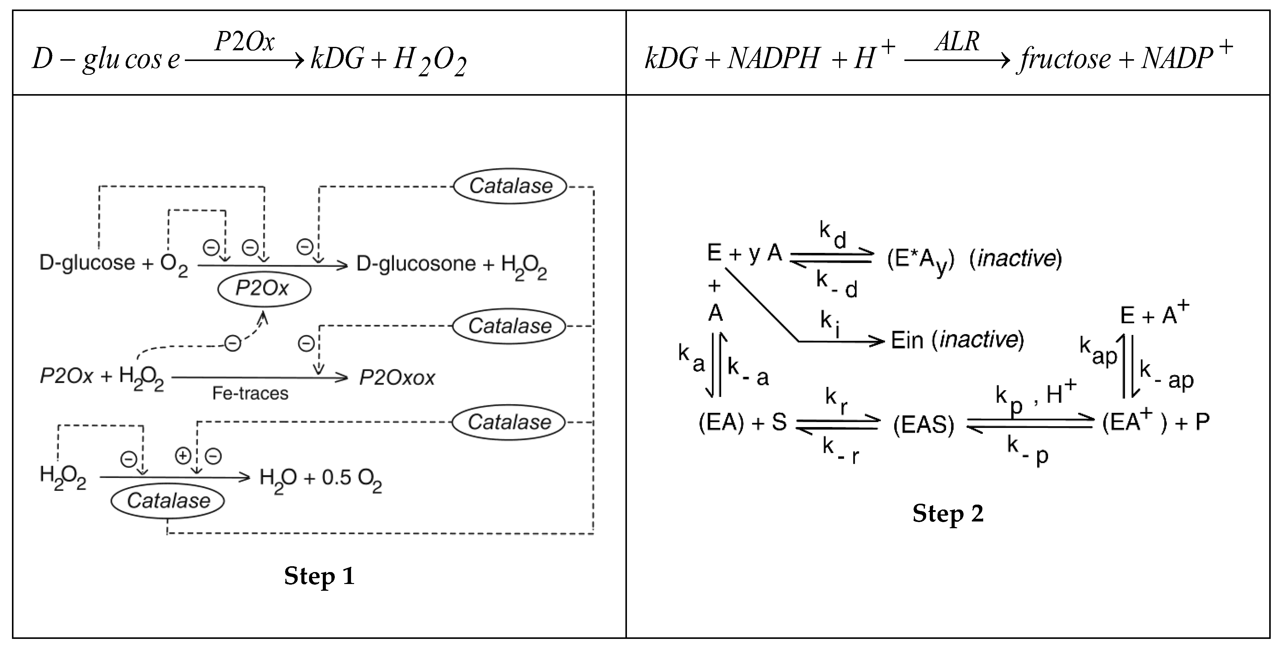
Figure 2.
Simplified reaction scheme of the inulin (S) hydrolysis to fructose (F) by using suspended inulinase (E, ENZ). After [68,69].
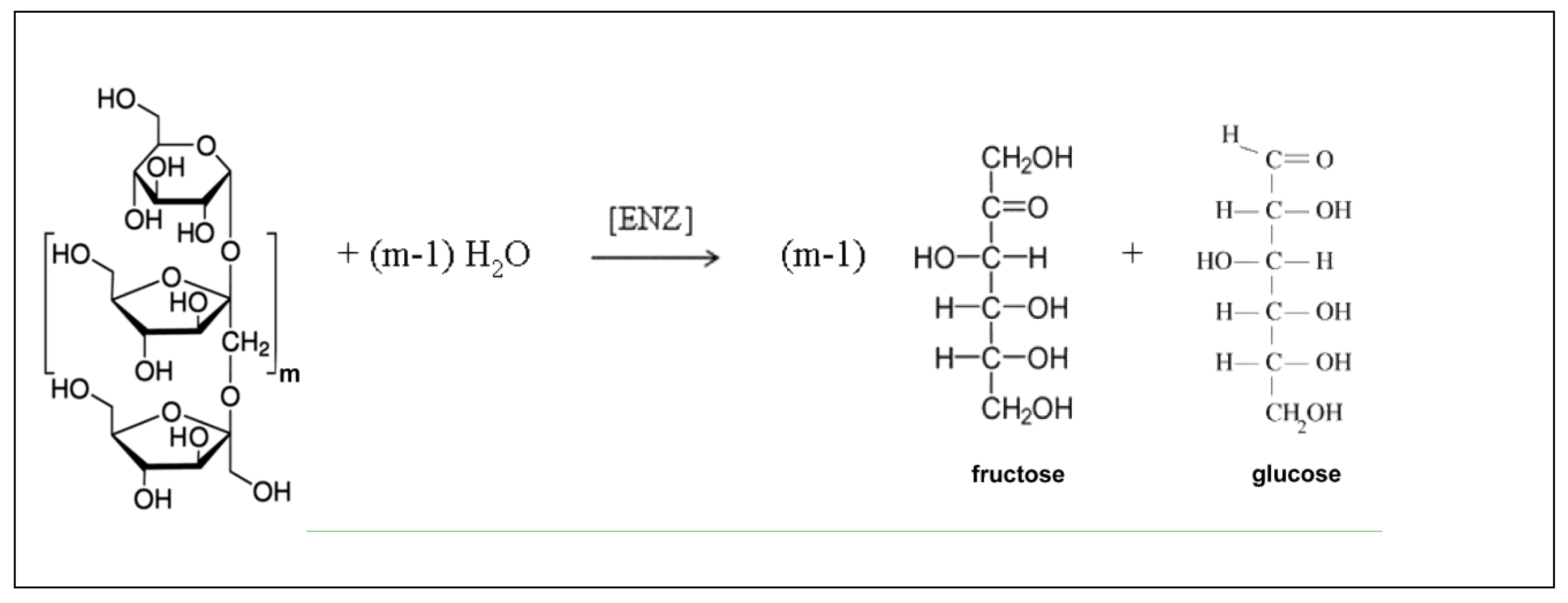
Table 1.
Comparison between three enzymatic methods used for the fructose synthesis.
| Characteristics |
Glucose isomerization [a,d] |
Cetus two steps process [b] | Inulin hydrolysis [c] |
| Number of steps | 1 | 2 | 1 |
| Conversion (%) | 50 (limited by the equilibrium) [d] |
99 | 99.5 |
| Raw-materials availability | Glucose from the starch of crops, mollases, cellulose, and food processing byproducts [Kanagasabai etal.,2023; Akbas and Stark,2016] | genetically modified chicory crop; cultures of Aspergillus sp. | |
| Impurities in the product | yes | traces | negligibles |
| Reaction type | Enzymatic isomerization | Enzymatic oxidation (step 1), followed by enzymatic reduction (step 2) | Enzymatic hydrolysis |
| Enzyme mobility | Immobilized [d] | Free (suspended) | immobilized |
| Enzyme stability, and other additives | Intra-cellular glucose-isomerase (e.g. Streptomyces murinus) of low stability; metal (Al) salts |
Pyranose 2-oxidase (P2Ox) and catalase (step 1); aldose reductase and NAD(P)H (step 2); enzymes are very costly |
Inulinase |
| Temperature | 50-60oC | 25-30oC (50-60oC)/ 30oC |
55oC (40-60oC) |
| Reaction time | 7 h | 3-20 h (step 1); 25 h (step 2) |
13 h |
| pH | 7-8.5 | 6.5-7(-8.5); 7-8.5 |
5.5 |
| Number of reaction steps | 1 isomerization |
2 oxidation (step 1), reduction (step 2) |
1 hydrolysis |
| Coenzyme necessary? | No | yes catalase for (step 1) to prevent P2Ox quick inactivation; NAD(P)H for step 2. NAD(P)H is continuously in-situ regenerated |
No |
| Product purification | Difficult [d] | simple (due to high selectivity) | simple (due to high selectivity) |
| Product purity | 2-5% impurities [d] | High (99.9%) |
High (99.9%) |
[a] Process described by [48,67]. The raw-material HFCS is obtained from yeast hydrolysis (resulting a mixture of 42% fructose, 50% glucose, and 8% other sugars)[48]. [b] Process described by [52,53,55,56,64]; NAD(P)H is continuously in-situ regenerated [59]. [c] Process described by [66,67,68,69]. [d] “This process suffers from a large number of disadvantages, as followings: i) The reaction is thermodynamically limited to around 50% glucose conversion, making the subsequent fructose separation in large chromatographic columns to be very costly. ii) Glucose isomerase is an intracellular enzyme with relatively poor stability, making its purification and immobilisation very difficult. iii) The amylase used to carry out the starch saccharification (to obtain the HFCS raw-material) requires calcium ions for full activity, but calcium inhibits glucose isomerisation, requiring its removal by ion-exchange treatment prior to glucose isomerisation. iv) The fructose product is still impurified by several other saccharides (such as aldose which is an allergenic compound).” [67,89,90,91,92,93].
Table 2.
Nominal operating conditions of the BR reactor, and its characteristics for the inulin hydrolysis case. Reaction conditions are those of Rocha et al. [71], and Ricca et al. [68,69][a].
| Operating conditions | Value | Remarks |
| Reactor liquid volume | 1 L (initial) | Up to 10 L capacity |
| Temperature / pressure / pH (buffer solution) | 50-55oC / normal / 4.5-5 | Batch time ( tf ) = 780 min. |
| Initial concentrations of Ricca et al. [69] | [S]o = 40 (g/L) [E]o = 97 (U/L) [W]o = 988.4 (g/L) [F]o = 0; [G]o = 0 |
To be optimized within imposed limits (this paper) |
| Optimization limits of control variables (initial BR, or in the FBR feeding)[68] [b,c,d] | [S]o; [S]in ∈ [40-200] g/L [E]o; [E]in ∈ [97-5500] (U/L) [W]o ∈ [988- 4000](g) FL ∈ [5e-4 – 0.01] (L/min) |
For FBR optimization, the W amount depends on the inlet feed flow rate (FL) of aqueous solution |
| Fructose polimerization degree in the inulin (m) | 29 (adopted) | 27-29 Inulin from chicory |
| Number of time-arcs for the optimized FBR (Ndiv) | 5 | FBR with variable feeding |
| Imposed inulin (S) conversion | Min. 90 % | |
| Inulin solubility [b] | 60 g/L (10oC) 160– 400 g/L (50oC), 330 g/L (90oC) | [67,70,74] |
| Inulin solutions viscosity, density [a] | Comparable to those of water | For [S] < 100 g/L [72,73] |
| Fructose solubility | 4000 g/L (ca. 22.2 M) (25°C) | [https://en.wikipedia.org/wiki/Fructose] |
| Glucose solution solubility | 5-7M (25-30oC) | [94] |
| Glucose / fructose solution viscosity | Ca. 1-3 cps (for up to 0.3 M) 1000 cps (4.5M, 30oC) |
[95] |
[a].- “Physical liquid properties correspond to a solution of inulin (S) and fructose (F), of densities and viscosities given by [77,78,96]. Glucose is present in small concentrations, and its properties have been assimilated with those of fructose. Molecular weights are: MF = 180.16 g/mol; MS ≈ 504-5,500 g/mol [https://link.springer.com/referenceworkentry/10.1007/978-3-319-03751-6_80-1]. [b].- Higher concentrations of inlet inulin solution have also been reported (up to 200 g/L, [71]). The inulin solubility depends on its source, and purification method, varying from 60 g/L at 10oC, to 160-400 g/L at 50oC, and more than 330 g/L at 90oC [67,70]. [c].- Maximum enzyme activity is reported as being of ca. 3000 U/mL (from K. marxianus var. marxianus CBS 6556), and of ca. 58000 U/g (from Trametes multicolor, [67]). [d].- One unit (U) of inulinase activity is defined as the amount of enzyme necessary to produce 1 μmoles fructose by hydrolysis of inulin over 1 minute of reaction under the standard conditions of 60oC and pH=5.” [68].
Disclaimer/Publisher’s Note: The statements, opinions and data contained in all publications are solely those of the individual author(s) and contributor(s) and not of MDPI and/or the editor(s). MDPI and/or the editor(s) disclaim responsibility for any injury to people or property resulting from any ideas, methods, instructions or products referred to in the content. |
© 2025 by the authors. Licensee MDPI, Basel, Switzerland. This article is an open access article distributed under the terms and conditions of the Creative Commons Attribution (CC BY) license (http://creativecommons.org/licenses/by/4.0/).
Copyright: This open access article is published under a Creative Commons CC BY 4.0 license, which permit the free download, distribution, and reuse, provided that the author and preprint are cited in any reuse.


