Submitted:
17 February 2025
Posted:
18 February 2025
You are already at the latest version
Abstract
Artificial Neural Networks (ANNs) have been successfully applied to predict various parameters in extrusion processes. However, few studies were found that have demonstrated their use in predicting the pressure profile along a single-screw extruder, and in these studies, motor current demand and melt temperature were not used as input variables. In this study, Feedforward Artificial Neural Networks (FANNs) were applied to predict the pressure profile along a single-screw extruder. The input layer variables tested included motor current demand, melt temperature, screw speed, and die restriction, while the output layer variables evaluated were four pressure measurements at different zones of the extruder. Motor current demand explained most of the data variability, accounting for 97.1% of the total variability. Five FANN architectures were tested: two considered all four input variables, two excluded the melt temperature, and the last one included only motor current demand and screw speed. The most accurate model included all four input variables, achieving a mean squared error (MSE) of 0.0078 and a coefficient of determination (R2) of 0.9889 with the test data. The variation between models including or excluding melt temperature was only in the fourth decimal place for R2. The FANN model proved efficient in predicting the pressure profile in single-screw extruders. These results provide valuable insights for improving extruder control systems and reducing costs associated with replacing defective sensors.
Keywords:
extrusion
; feedforward artificial neural networks
; modeling
; polymers
; prediction
; pressure profile
1. Introduction
The global production of polymers is approximately 400 million tons per year (Plastics Europe, 2023). The equipment used in polymer processing consumes at least 60% of the total energy in the plant (Kent, 2018) and the specific energy required for its production is estimated to be around 0.5 (Estrada & Janna, 2022). The increasing complexity in polymer manufacturing, driven by applications in industries such as automotive and aerospace, has focused efforts on optimizing these processes to improve product quality and efficiency. This has promoted the adoption of Industry 4.0 protocols and in-line sensors, thus enhancing process understanding and improving data collection for computational models with a high degree of accuracy (Abeykoon et al., 2021).
The simulation of a process is recommended when it presents a high level of complexity or when no simple analytical model that offers sufficient precision is available (Carson, 2005); in such cases, data acquisition eases parameter adjustment or data-driven models in the simulation. Solving mathematical models for various unit operations through simulations is common in chemical engineering; additionally, they are used to optimize and design equipment (De Tommaso et al., 2020). In polymer processes, such as plastic extrusion, where polymer flow occurs under thermal gradients and is subjected to high shear rates, there have been advancements in the modeling of complex physical phenomena such as viscoelastic behavior and crystallization (Hyvärinen et al., 2020). In a single-screw extruder, heat transfer by conduction and viscous dissipation are the predominant sources of heat (Rauwendaal, 2016). Plastic extrusion is achieved by pumping a molten mass of polymers and shaping it through a forming die. A plasticizing unit functions as a pressure builder; its pressure profiles are critical because productivity and process stability depend on them. The most common equipment in the extrusion process is the single-screw extruder (Rauwendaal, 2018), which typically consists of three main zones: feeding or solid transport zone, melting or transition zone, and pumping or metering zone (Dyadichev et al., 2019; Kadyirov et al., 2019).
Modeling extrusion involves addressing phenomena such as solid transport, melting, fluid transport, and melt mixing, and each one presents its own complexity. Melt transport models can be classified into two main categories: one based on geometric and physical conditions, and the other based on the mathematical methodology used (Marschik et al., 2022).The extrusion process can be simulated using CFD (Computational Fluid Dynamics), where most solution methods can solve the Navier-Stokes equations that describe the conservation of mass, momentum, and energy (Hosain & Fdhila, 2015). CFD software such as Polyflow, developed by ANSYS, have been used recently to simulate single-screw and twin-screw plastic extruders. They predict variables such as residence time, shear stresses, flow patterns, and the variation of temperature and pressure along the screw (Hyvärinen et al., 2020). However, using CFD techniques could have a high computational cost or take too much time, thus hindering its implementation in plant operations (Udoewa & Kumar, 2012).
The growth in data availability and computing capacity, data analysis, and advancements in artificial intelligence have renewed some scientific disciplines. However, when analyzing biological, physicochemical, or engineering systems, data acquisition is often expensive; therefore, they become inaccessible and lead to decision making based on incomplete information. This issue can be addressed by leveraging prior knowledge on physical and biological phenomena that can serve as regulator to constrain the solution space for neural networks, resulting in a broader perspective for the algorithm based on the supplied data (Raissi et al., 2019). The development of sensors and the increase in data storage capacity provide the opportunity to apply physical laws using data; for instance, Feedforward Deep Neural Networks (PDE-Net) to solve partial differential equations, or Physics-Informed Neural Networks (PINNs) (Cai et al., 2021; Long et al., 2018). PINNs, also known as Physics-Informed Machine Learning (PIML), incorporate physical differential equations into the loss function (Faegh et al., 2025). Artificial Neural Networks (ANNs) are a branch of artificial intelligence (AI) and can be used in cases where parameters and mathematical models are lacking, or the models are too complex for the desired application.
The complexity of the phenomena in polymer processing makes its modeling and control more difficult; therefore, the use of artificial intelligence techniques such as expert systems, neural networks, and fuzzy logic, in particular, is more suitable in these cases (Abeykoon, 2016). For this type of problem, there are diverse types of ANNs such as multilayer perceptron (MLP) deep neural networks, which have nonlinear layers and are trained in a supervised manner. That is, input data is used along with their corresponding outputs, parameters are initialized randomly, and the neural network is trained using a gradient descent algorithm and backpropagation (Patel et al., 2018). When a validated model is available, it is possible to create a database under different operating conditions to train ANNs that can predict phenomena such as heat transfer (Kim et al., 2022).
Several studies have been conducted to predict pressure in the solid transport zone, the melting zone, and the addition zone; however, due to the simplifications made to find analytical solutions, they are unable to capture the dynamic changes in the process. Some authors have opted for soft computing techniques to model plastic extrusion. Mekras & Artemakis (2012) trained a deep neural network with two hidden layers using experimental data from a micro-extrusion process. They considered three input features and nine outputs for the ANN. By calculating most of the process parameters required for sizing a microtube and the type of material, they achieved an approximation with an error of less than 1%. Meißner et al. (2020) employed FANNs in the inverse problem of identifying material parameters in simulations of parts manufactured via material extrusion, specifically Acrylonitrile Butadiene Styrene (ABS). The training data consisted of force-displacement curves obtained from simulations using finite element methods. The objective was to predict these parameters to describe the elastic-plastic behavior of ABS under uniaxial loading, enabling efficient calibration of structural models.
Roland et al. (2021) predicted the nonlinear relationship between flow rate and pressure in single-screw extruders. They used ANN models, gradient boosted trees, and symbolic regression based on genetic programming. Their study relied on simulated data from ANSYS, modeling the melt transport of a non-Newtonian fluid with temperature-independent power-law behavior. They identified four independent parameters: the power-law exponent n, the dimensionless pressure gradient in the downstream channel, the screw pitch ratio, and the ratio of channel height to width, thus describing the flow rate prediction. Gaspar-Cunha et al. (2022) proposed the use of Artificial Intelligence techniques, such as DAMICORE, which is a data mining framework, to determine the interrelationship between design variables and objectives in plastic extrusion. Perera et al. (2023) trained an ANN with MLP architecture to predict the melting pressure and achieved good predictive performance with a normalized mean squared error of 0.045 ± 0.003. Furthermore, they found that there are no previous works on predicting melting pressure using deep learning techniques.
A model based on FANNs is being developed to predict the pressure profile along a single-screw extruder in polymer extrusion processing. According to the literature, no previous studies were found that consider the use of motor current demand and melt temperature as input variables in ANNs models. This approach is highly beneficial in the extrusion industry, especially because pressure sensors are expensive devices that often are not adequately replaced when they fail, thus compromising quality, process consistency, and safety. Moreover, despite the significance of melting pressure in controlling the extrusion process, there are limitations in current studies that effectively address the prediction of pressure profiles through advanced modeling techniques. The use of ANNs enables capturing the complex interactions between process variables and generating accurate predictions based on historical data. This not only presents a cost-effective solution in the absence of sensors but also provides a powerful tool for real-time process optimization and control. This study aims to provide a robust and highly accurate predictive model that could be easily implemented in polymer extrusion plants, thereby improving operational efficiency and reducing costs associated with replacing failed sensors.
2. Methodology
2.1. Process Description and Model Objective
Experimental data collection was carried out on a EXTRUDEX EN045-30 single-screw extruder with a conventional screw and a smooth feed zone. The barrel diameter is 45 mm, the length to diameter ratio is 30, and the channel width is 41.1 mm. The screw radius , the barrel radius , and channel height are shown in Figure 1. Table 1 presents the barrel and die temperature profile , the length at which it is located along the extruder, and the heating zone in which it is found. Each temperature has an independent control system.
In the extrusion process, there are four independent variables: the material, barrel and die temperature profile , screw rotational speed , and die restriction , the last three are controlled within the extruder (Estrada et al., 2020). Barrel temperature and rotational screw speed variables affect the melting pressure development in the extruder (Abeykoon et al., 2011). In this study, was not considered but the impact of other measured variables such as motor current demand , rotational screw speed , melting temperature and die restriction was evaluated. Table 2 shows the distance of the pressure sensors and the zone in which they were located on the extruder. Figure 2 shows the location of the pressure sensors, the heating zones in the extruder, and the set of thermocouples in the die to measure the melting temperature (Thermocomb). To collect data on the pressure profile along the extruder, four Dynisco® pressure transducers were installed, as shown in Table 2. is determined by the mandrel protruding from the end of the extruder, which ranges from 0 to 10 turns, where 0 turns mean fully restricted, and 10 turns means no restriction. Each turn is graduated between 0 and 360, with increments of 15.

Table 2.
Pressure sensors along the extruder.
| No. | Zone | Dynisco® Model | Class | Range [bar] | |
| 1 | 10.3 D | Solid Conveying | MDA420-1/2-1.4M-15 | 1 | 0-1400 |
| 2 | 18.3 D | Melting | MDA420-1/2-1.4M-15 | 1 | 0-1400 |
| 3 | 26.3 D | Melting | MDA420-1/2-1.4M-15 | 1 | 0-1400 |
| 4 | 35.2 D | Melt Flow in the Die | Dyna-4-5c-T80 | 1 | 0-500 |
For experimental data collection, virgin polypropylene (PP) homopolymer, commercially known as ESENTTIA 05H82-AV, was used. The melt flow index (MFI) is 4.80 at 230 °C – 2.16 kg (Esenttia, 2021). The density of PP is 0.906 g/cm³, determined using the ISO 1183-1:2019 method and the melting point is 164.87 °C, measured with a TA - Instruments DSC Q200 using the ASTM D 3418-21 method. and were measured using sensors integrated into the extruder control system. The temperature profile was kept constant during the runs.
The developed model seeks to predict the pressure profile along a single-screw extruder using a FANN. The considered input variables were , , , and . Since direct measurement of presents difficulties due to its contact with the molten polymer, the model seeks to explore whether it is possible to obtain accurate predictions by excluding this variable, leveraging the implicit relationships that may have with other inputs. In this way, the model aims to optimize extrusion monitoring and reduce the need for complex temperature sensors without compromising the accuracy of pressure predictions at key points in the extruder.
2.2. Data Collection and Processing
The sensors used during data acquisition were calibrated before operation, which minimized out-of-range data. Data were collected by varying the between 0 and 160 , implementing speed change ramps from 0 to 40, then from 40 to 100 , and finally from 100 to 160 . was modified between 4.08 and 4.46 to achieve the desired melting pressures. Experimental data collection was carried out in different sessions to ensure variability in the information, and then data were combined into a single dataset. The extruder’s software was configured to collect data at 1-second intervals, resulting in a total of 66,846 data points. System perturbations were conducted each time the process reached a steady state, after waiting for 12 to 15 minutes. During data processing, adjustments were made to the data acquired by the thermocouple array in the die (Thermocomb) and to the data collected with sensors No. 1 and 2. For the , due to the presence of 57 out-of-range samples in one of the runs, these values were replaced using linear interpolation, allowing for an estimation based on the adjacent data. Regarding the data, some negative values were obtained from sensors No. 1 and 2, as the pressures reached in the solids conveying zone and at the start of the melting zone can be low and affect the sensitivity of the sensors. These data were substituted using linear interpolation based on neighboring values. In the end, the same initial number of data points was preserved for model development. The experimental data for , , and were used as inputs to the model. Figure 3 shows the experimental dataset after processing.
Principal Component Analysis (PCA) is a traditional dimensionality reduction technique that assumes that the observed data are a linear combination of a certain basis. Abdi & Williams (2010) described the development of this multivariate statistical technique. In this analysis, variables were first normalized using the mapminmax method [-1,1], which is given by Equation (1):
where are the normalized data, are the measured data values, and and represent the minimum and maximum values of the measured data, with and set to 1 and -1, respectively. PCA was then applied to the input variables of the model, as shown in Figure 4, and revealed that the linear correlation between the variables is weak; dark red indicates a strong correlation between the variable and the principal component, while light blue corresponds to a weak correlation between the variable and the principal component. The analysis shows that and have a moderate positive correlation of 0.20, thus indicating that as the motor current demand increases, the rotational screw speed also increases. Additionally, the has a negative correlation with both (-0.13) and (-0.22), suggesting that an increase in motor current demand may be associated with a slight decrease in these variables. and have an inverse relationship with a value of -0.3. In turn, the rotational screw speed and die restriction have a very low correlation. Lastly, it is shown that and have a negative correlation (-0.26), thus indicating an inverse relationship.
The analysis of total explained variance is described by Jollife & Cadima (2016) and shows that it is common to use a specific percentage, e.g., 70%, to decide how many principal components (PC) should be retained, although this threshold is subjective. Nevertheless, this percentage remains key to evaluate the quality of graphical representations. While the first components are often emphasized in the analysis, the last ones can also be useful, especially in outlier detection or in some image analysis applications. Figure 5 shows that explains most of the data variability, accounting for 97.1% of the total variability. (1.8%), (1.0%), and (0.0%) do not significantly contribute to the explained variance. This suggests that motor current demand has a primary role in the model, while the other variables are secondary.
2.3. Feedforward Artificial Neural Networks
Data were randomly divided to ensure that there are no patterns related to the order in which they were combined; thereby reducing the risk of overfitting by guaranteeing that the training and test data were representative. Additionally, a seed was added so that the data generation is consistent in each trial. The dataset was split with 70 % allocated for training, 15% for validation, and the remaining 15 % for testing. Five configurations of FANNs were tested. Furthermore, the extrusion process has been modeled based on a 1D hyperbolic PDE analysis of mass transport (Diagne et al., 2016b, 2016a). When solving PDEs with PINNs, Wang et al. (2023) recommend initially using the hyperbolic tangent activation function, which is given by Equation (2):
Its range is [-1, 1]. The hyperbolic tangent was used as the activation function in this model. The values of the weights ( and the biases were initialized randomly. Mean Squared Error and the Coefficient of Determination were used as metrics to evaluate the accuracy of the model, as shown in Equations (3) and (4) :
where is the number of data points, is the predicted output, and is the mean value of the observed data. The Levenberg-Marquardt backpropagation algorithm was used as optimizer. It is a variant of traditional backpropagation that utilizes an approximation of the Newton method to update the weights of a neural network using the Hessian matrix and gradient (Bilski & Wilamowski, 2017).
Models were trained and validated on a Lenovo Legion 5 Pro laptop with an 11th Gen Intel(R) Core (TM) i7-11800H @ 2.30GHz processor (16 CPUs) and 32 GB of RAM. The programming language MATLAB, version 24.2.0.2712019 (R2024b), was used for the training and validation of the FANNs model. ANNs modelling has been studied to improve their performance, focusing on the data collection process for training, data processing, activation functions, weight initialization, optimizers, and error functions. Additionally, efforts have been made to improve the architecture of ANNs; however, there is no theoretical basis for this, although some methods can be used in specific cases (Benardos & Vosniakos, 2007). In this work, the general method of trial and error was employed.
3. Results and Discussion
Table 3 presents the architectures tested in the FANNs used to predict the pressure profile along a single-screw extruder, the values obtained for the metrics used to evaluate the accuracy of the model ( and ) for each dataset (training, validation, testing, and overall), the number of neurons per layer (), as well as the number of epochs () and the computational time () required for training each proposed architecture. No learning rate was entered into the model since the 'trainlm' (Levenberg-Marquardt) algorithm in MATLAB adjusts the learning rate directly. It uses an adaptive value called , which increases when an iteration raises the performance function and decreases after each successful step (reduction in the performance function). The default value of is 0.001, the decrease factor is 0.1, the increase factor is 10, and the maximum value is . The input variables used in the FANNs are , , and . The outputs of the FANNs are the predicted pressure profiles at four points along the extruder (, , , ) as indicated in Table 2.
The training results of the different FANNs architectures yielded low values ranging from 0.0075 to 0.0261, values varied between 0.9623 and 0.9894, thus indicating a high model fitting capability. In the validation and test datasets, values ranged from 0.0078 to 0.0255, and values were between 0.9631 and 0.9889, demonstrating a strong predictive capacity of the models. Additionally, there is a minimal difference between the values obtained from the training dataset compared to those of the validation and test datasets, which suggest that tested models do not present overfitting. In general, it is observed that values are consistently high in all cases, indicating that FANNs have been able to adequately model the relationship between input variables and pressure profile in the extruder. Despite variations in the number of neurons in hidden layers 1 and 2, there is not a significant difference in and among tested architectures; therefore, these factors do not have a substantial impact on model performance.
The specific mechanical energy (SME) is an indicator of the extrusion process and is derived from independent variables such as barrel temperature, rotational screw speed, and die geometry (Fayose & Huan, 2014). In a study on the energy consumption by a single-screw extruder conducted by Abeykoon et al. (2010), they found that the rotational screw speed is the most significant parameter in determining the motor energy demand. As shown in the analysis of the percentage of variance explained in Figure 5, explains 97.1% of the total data variability. Therefore, architectures were tested, and greater importance was given to the variable as an input to the model. The first and second architectures shown in Table 4 consider the four measured variables in the extruder (, , and ) as model inputs. The first FANN achieved the highest performance of all tests. The measurement of involves direct contact with the melt inside the extruder, unlike the variables , , and , which are external measurements that do not require direct contact with it. In the third and fourth architectures, the variable was excluded, and it was observed that omitting this variable only slightly decreased the accuracy of the model; the best results were obtained in the third architecture. In the last two tested architectures, only and were used as model inputs, thus showing that excluding from the model reduced the prediction accuracy, as it plays an important role in controlling the material flow in the die, directly affecting the pressure profile.
The third FANN in Table 4 is of particular interest because it uses only , , and as input variables, omitting , which offers a significant advantage by reducing the number of input variables required by the FANN for pressure profile prediction. Additionally, is not frequently measured in industrial environments. Regarding performance, this architecture shows an of 0.9867 for the training set, 0.9861 for the validation set, and 0.9863 for the test set, with values ranging from 0.0093 to 0.0097 across all datasets. The number of epochs and convergence time yielded values of and . These indicate high prediction accuracy, even without considering melting temperature as an input variable. It is possible that the effect of on the pressure profile is indirectly captured by variables such as , and , which are related to heat transfer and the rheological behavior of the polymer during the extrusion process. The die restriction is a material flow control element that directly affects the pressure profile within the extruder, it determines how the material is transported and heated during the process. It has been found that viscous dissipation caused by shear contributes approximately 80% of the heat needed to melt the polymer (Hyvärinen et al., 2020). imposes pressure due to the resistance that must be overcome, which increases dissipation and, consequently, material temperature. By including in the model, the FANN gains indirect information on the behavior of , as and the flow respond to the pressure demand at the die, adapting internal flow and temperature conditions to meet this restriction. In this way, plays an important role in process dynamics, becoming as significant as , and providing the necessary information for the FANN to make more accurate predictions without explicitly requiring . This FANN’s diagram is shown in Figure 6.
The equation that defines this FANN shown in Figure 6 and is obtained as follows:
Hidden layer 1:
Activation function of hidden layer 1:
Hidden layer 2:
Activation function of hidden layer 2:
Output layer:
Activation function of output layer:
where is the identity matrix, , and are the weight matrices from the input layer to the first hidden layer, from the first hidden layer to the second hidden layer, and from the second hidden layer to the output layer, respectively. , , and are the bias vectors for the first hidden layer, second hidden layer, and output layer, respectively. By substituting and into , we obtain:
Equation (11) represents the general equation of a FANN with three layers. The FANN of interest has inputs , , and , and its architecture is defined by 3 , 10 neurons in the first hidden layer , 8 neurons in the second hidden layer , and 4 neurons in the output layer . Parameters have the following dimensions: , , , , and , resulting in a total of 164 parameters, including weights and biases, that need to be adjusted to improve the performance of the network.
Figure 7 presents the actual pressure data (in blue) and the predictions (in red) made by the FANN. There is lower precision in the prediction of , which corresponds to the solid transport zone that extends to where the solid plug reaches the melting point. In this zone (delay zone), the melting mechanism has a delay, which is where the first traces of molten material are generated (Kacir & Tadmor, 1972). Therefore, with only a thin film of molten material, there is greater noise in the measurement. This same issue is observed for , as the sensor is located in the melting zone, but with a greater presence of molten material, the noise decreases. is positioned at the end of the melting zone, which is why there is very little noise in the measurement, as the polymer is almost entirely molten. The prediction for , located at the end of the solid transport zone and the beginning of the molten flow zone in the die, is very high. Actual data nearly overlaps the predictions made by the FANN completely. In this area, the polymer is fully molten, thus eliminating the noise caused by the presence of solids, leaving only the inherent measurement noise. It is noteworthy that (melt pressure) is the measurement of greatest interest in the process as a quality parameter for the product (Abeykoon et al., 2020). Therefore, the model aims to achieve the highest prediction accuracy for this measure.
The accuracy demonstrated by the FANN highlights the potential of these models to predict process variables like the pressure profile in a single-screw plastic extruder. This performance also opens the possibility of real-time implementation within the process control system, as ANNs can function effectively as soft sensors. Such sensors are a cost-effective alternative to expensive physical sensors, can easily complement physical sensors, and can be applied directly while continuously evaluating data during operation (Savytskyi et al., 2020). The implemented FANN showed a high capacity to capture dynamic changes occurring in the process in response to disturbances, thus making them a valuable tool for assessing energy efficiency and optimizing energy consumption.
Traditional machine learning models face limitations with low data availability; various solutions have been proposed to address this, e.g., data augmentation through slight modifications of existing data; embedding domain knowledge into the structure of FANNs using white-box models that integrate physical laws or black-box models, which require extensive data; integration of differential equations to supplement missing data in PINNs as a solution to this challenge (Buchaniec et al., 2021). Feng et al. (2019) demonstrated that deep and narrow neural networks can address problems in material science, where data availability is often limited. They suggest specific training methods, such as pre-training with a stacked autoencoder in deep neural networks (DNN) using a small dataset. Finally, applying artificial neural network models to new materials, operating conditions and different equipment can reduce prediction accuracy, or make adaptation challenging if there is not enough data reflecting these changes in the process.
4. Conclusions
In this work, the use of FANNs was proposed to predict the pressure profile in a single-screw plastic extruder, including motor current demand and melt temperature as input variables. Based on the model performance, the potential of ANNs as soft sensors is highlighted, presenting them as an alternative to physical sensors when these fail or need replacement, thus enabling uninterrupted process control and continuous plant operation. Despite limitations such as the requirement for large datasets, application to different materials, and changes in extruder geometry, ANNs can play a significant role in process optimization and real-time monitoring.
Motor current demand () is an impornant input variable for the ANN model when predicting the pressure profile due to its correlation with polymer transport during the extrusion process. Additionally, as it accounts for most of the variance in the data, including it in the model ensures high prediction accuracy. In addition, it is shown that including as an input variable in the ANN model increases the accuracy in predicting the pressure profile along the single-screw extruder; since this variable plays a key role in flow dynamics within the die, its absence results in a significant loss of prediction accuracy. It is recommended that this variable continue to be used in future analyses and industrial applications.
Acknowledgments
The authors thank the Ministry of Science and Technology - MINCIENCIAS for co-financing the project “Development of new advanced technologies of industry 4.0 for SMEs and MSMEs for polymer processing to increase energy and productive efficiency” through contract 127-2022. The first author also acknowledges Esenttia S.A. for providing the material for testing and Instituto de Capacitación e Investigación del Plástico y del Caucho (ICIPC) for supporting the collection of experimental data.
Nomenclature
| Symbol | Description | Units |
| Activation function | - | |
| Bias | - | |
| Barrel diameter | ||
| Epochs | - | |
| Channel height | ||
| Hidden layer | - | |
| Identity matrix | ||
| Input variables | - | |
| Motor current demand | ||
| Input layer | - | |
| Weight matrix from the input layer to the first hidden layer | - | |
| Length | ||
| Weight matrix from the first hidden layer to the second hidden layer | - | |
| Weight matrices from the second hidden layer to the output layer | - | |
| Mean squared error | - | |
| Number of data points | - | |
| Number of neurons | - | |
| Activation function of output layer | - | |
| Output layer | - | |
| Output variables | - | |
| Pressure | ||
| Screw radius | ||
| Coefficient of Determination | - | |
| Die restriction | ||
| Time | ||
| Melting temperature | ° | |
| Barrel and die temperature profile | ° | |
| Channel width | ||
| Weights | - | |
| Maximum value of the measured data | - | |
| Minimum value of the measured data | - | |
| Measured data | - | |
| Normalized data | - | |
| Mean value of the observed data | - | |
| Predicted output | - | |
| Maximum value of the normalized data | - | |
| Minimum value of the normalized data | - | |
| Greek symbols | ||
| Adaptive learning rate | - | |
| Rotational screw speed | ||
References
- Abdi, H., & Williams, L. J. (2010). Principal component analysis. In Wiley Interdisciplinary Reviews: Computational Statistics (Vol. 2, Issue 4, pp. 433–459). [CrossRef]
- Abeykoon, C. (2016). Single screw extrusion control: A comprehensive review and directions for improvements. Control Engineering Practice, 51, 69–80. [CrossRef]
- Abeykoon, C., Li, K., Martin, P. J., & Kelly, A. L. (2011). Modelling of melt pressure development in polymer extrusion: Effects of process settings and screw geometry. Proceedings of 2011 International Conference on Modelling, Identification and Control, ICMIC 2011, 197–202. [CrossRef]
- Abeykoon, C., McAfee, M., Li, K., Martin, P. J., Deng, J., & Kelly, A. L. (2010). Modelling the Effects of Operating Conditions on Motor Power Consumption in Single Screw Extrusion (pp. 9–20). [CrossRef]
- Abeykoon, C., McMillan, A., & Nguyen, B. K. (2021). Energy efficiency in extrusion-related polymer processing: A review of state of the art and potential efficiency improvements. In Renewable and Sustainable Energy Reviews (Vol. 147). Elsevier Ltd. [CrossRef]
- Abeykoon, C., Pérez, P., & Kelly, A. L. (2020). The effect of materials’ rheology on process energy consumption and melt thermal quality in polymer extrusion. Polymer Engineering and Science, 60(6), 1244–1265. [CrossRef]
- Benardos, P. G., & Vosniakos, G. C. (2007). Optimizing feedforward artificial neural network architecture. Engineering Applications of Artificial Intelligence, 20(3), 365–382. [CrossRef]
- Bilski, J., & Wilamowski, B. M. (2017). Parallel Levenberg-Marquardt Algorithm Without Error Backpropagation. Springer International Publishing ICAISC 2017, Part I, LNAI, 10245, 25–39. [CrossRef]
- Buchaniec, S., Gnatowski, M., & Brus, G. (2021). Integration of classical mathematical modeling with an artificial neural network for the problems with limited dataset. Energies, 14(16). [CrossRef]
- Cai, S., Wang, Z., Wang, S., Perdikaris, P., & Karniadakis, G. E. (2021). Physics-informed neural networks for heat transfer problems. Journal of Heat Transfer, 143(6). [CrossRef]
- Carson, J. S. (2005). Introduction to modeling and simulation. Proceedings of the Winter Simulation Conference, 2005., 8 pp.-. [CrossRef]
- De Tommaso, J., Rossi, F., Moradi, N., Pirola, C., Patience, G. S., & Galli, F. (2020). Experimental methods in chemical engineering: Process simulation. In Canadian Journal of Chemical Engineering (Vol. 98, Issue 11, pp. 2301–2320). Wiley-Liss Inc. [CrossRef]
- Diagne, M.; Shang, P.; Wang, Z. (2016a). Feedback Stabilization for the Mass Balance Equations of an Extrusion Process. IEEE Transactions on Automatic Control, 61(3), 760–765. [CrossRef]
- Diagne, M.; Shang, P.; Wang, Z. (2016b). Well-posedness and exact controllability of the mass balance equations for an extrusion process. Mathematical Methods in the Applied Sciences, 39(10), 2659–2670. [CrossRef]
- Dyadichev, V. V.; Kolesnikov, A. V.; Menyuk, S. G.; Dyadichev, A. V. (2019). Improvement of extrusion equipment and technologies for processing secondary combined polymer materials and mixtures. Journal of Physics: Conference Series, 1210(1). [CrossRef]
- Esenttia. (2021). 05H82-AV - Esenttia S.A. https://www.esenttia.co/zp/api/webroot/productos/BT_Espanol/BT_ES_05H82-AV.pdf.
- Estrada, O.; Janna, F. C. (2022). A novel melting model for polymer extrusion: Mechanically induced transition layer removal. Polymer Engineering and Science, 62(10), 3290–3309. [CrossRef]
- Estrada, O.; Ortiz, J. C.; Hernández, A.; López, I.; Chejne, F.; del Pilar Noriega, M. (2020). Experimental study of energy performance of grooved feed and grooved plasticating single screw extrusion processes in terms of SEC, theoretical maximum energy efficiency and relative energy efficiency. Energy, 194. [CrossRef]
- Faegh, M.; Ghungrad, S.; Oliveira, J. P.; Rao, P.; Haghighi, A. (2025). A review on physics-informed machine learning for process-structure-property modeling in additive manufacturing. Journal of Manufacturing Processes, 133, 524–555. [CrossRef]
- Fayose, F. T.; Huan, Z. (2014). Specific mechanical energy requirement of a locally developed extruder for selected starchy crops. Food Science and Technology Research, 20(4), 793–798. [CrossRef]
- Feng, S.; Zhou, H.; Dong, H. (2019). Using deep neural network with small dataset to predict material defects. Materials and Design, 162, 300–310. [CrossRef]
- Gaspar-Cunha, A.; Monaco, F.; Sikora, J.; Delbem, A. (2022). Artificial intelligence in single screw polymer extrusion: Learning from computational data. Engineering Applications of Artificial Intelligence, 116. [CrossRef]
- Hosain, M. L.; Fdhila, R. B. (2015). Literature Review of Accelerated CFD Simulation Methods towards Online Application. Energy Procedia, 75, 3307–3314. [CrossRef]
- Hyvärinen, M.; Jabeen, R.; Kärki, T. (2020). The modelling of extrusion processes for polymers-A review. In Polymers (Vol. 12, Issue 6). MDPI AG. [CrossRef]
- Jollife, I. T.; Cadima, J. (2016). Principal component analysis: A review and recent developments. In Philosophical Transactions of the Royal Society A: Mathematical, Physical and Engineering Sciences (Vol. 374, Issue 2065). Royal Society of London. [CrossRef]
- Kacir, L.; Tadmor, Z. (1972). Solids Conveying in Screw Extruders Part 111: The Delay Zone". Polymer Engineering and Science, 12, 387–395. [CrossRef]
- Kadyirov, A.; Gataullin, R.; Karaeva, J. (2019). Numerical simulation of polymer solutions in a single-screw extruder. Applied Sciences (Switzerland), 9(24). [CrossRef]
- Kent, R. (2018). Targeting and controlling energy costs. In Energy Management in Plastics Processing (pp. 79–104). Elsevier. [CrossRef]
- Kim, D. J.; Kim; Il, S.; Kim, H. S. (2022). Thermal simulation trained deep neural networks for fast and accurate prediction of thermal distribution and heat losses of building structures. Applied Thermal Engineering, 202. [CrossRef]
- Long, Z.; Lu, Y.; Ma, X.; Dong, B. (2018). PDE-Net: Learning PDEs from Data. In International conference on machine learning (pp. 3208–3216). PMLR.
- Marschik, C.; Roland, W.; Osswald, T. A. (2022). Melt Conveying in Single-Screw Extruders: Modeling and Simulation. In Polymers (Vol. 14, Issue 5). MDPI. [CrossRef]
- Meißner, P.; Watschke, H.; Winter, J.; Vietor, T. (2020). Artificial neural networks-based material parameter identification for numerical simulations of additively manufactured parts by material extrusion. Polymers, 12(12), 1–28. [CrossRef]
- Mekras, N.; Artemakis, I. (2012). Using artificial neural networks to model extrusion processes for the manufacturing of polymeric micro-tubes. IOP Conference Series: Materials Science and Engineering, 40(1). [CrossRef]
- Patel, H.; Thakkar, A.; Pandya, M.; Makwana, K. (2018). Neural network with deep learning architectures. Journal of Information and Optimization Sciences, 39(1), 31–38. [CrossRef]
- Perera, Y. S.; Li, J.; Kelly, A. L.; Abeykoon, C. (2023). Melt Pressure Prediction in Polymer Extrusion Processes with Deep Learning. IEEE.
- (2023). Plastics - the fast Facts 2023. https://plasticseurope.org/knowledge-hub/plastics-the-fast-facts-2023/.
- Raissi, M.; Perdikaris, P.; Karniadakis, G. E. (2019). Physics-informed neural networks: A deep learning framework for solving forward and inverse problems involving nonlinear partial differential equations. Journal of Computational Physics, 378, 686–707. [CrossRef]
- Rauwendaal, C. (2016). Heat transfer in twin screw compounding extruders. AIP Conference Proceedings, 1779. [CrossRef]
- Rauwendaal, C. (2018). Understanding Extrusion. https://doi.org/10.3139/9781569906996. [CrossRef]
- Roland, W.; Marschik, C.; Kommenda, M.; Haghofer, A.; Dorl, S.; Winkler, S. (2021). Predicting the Non-Linear Conveying Behavior in Single-Screw Extrusion: A Comparison of Various Data-Based Modeling Approaches used with CFD Simulations. International Polymer Processing, 36(5), 529–544. [CrossRef]
- Savytskyi, O.; Tymoshenko, M.; Hramm, O.; Romanov, S. (2020). Application of soft sensors in the automated process control of different industries. E3S Web of Conferences, 166. [CrossRef]
- Udoewa, V.; Kumar, V. (2012). Computational Fluid Dynamics. In Applied Computational Fluid Dynamics. InTech. [CrossRef]
- Wang, S.; Sankaran, S.; Wang, H.; Perdikaris, P. (2023). AN EXPERT’S GUIDE TO TRAINING PHYSICS-INFORMED NEURAL NETWORKS. ArXiv, abs/2308.08468.
Figure 1.
Screw geometry.
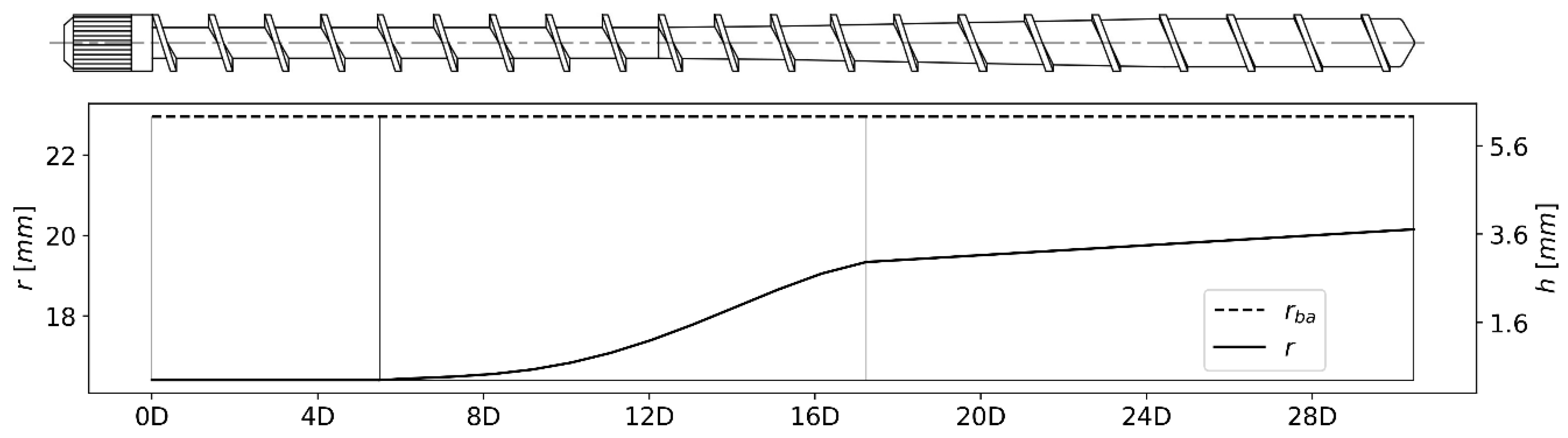
Figure 2.
Single-screw extruder.
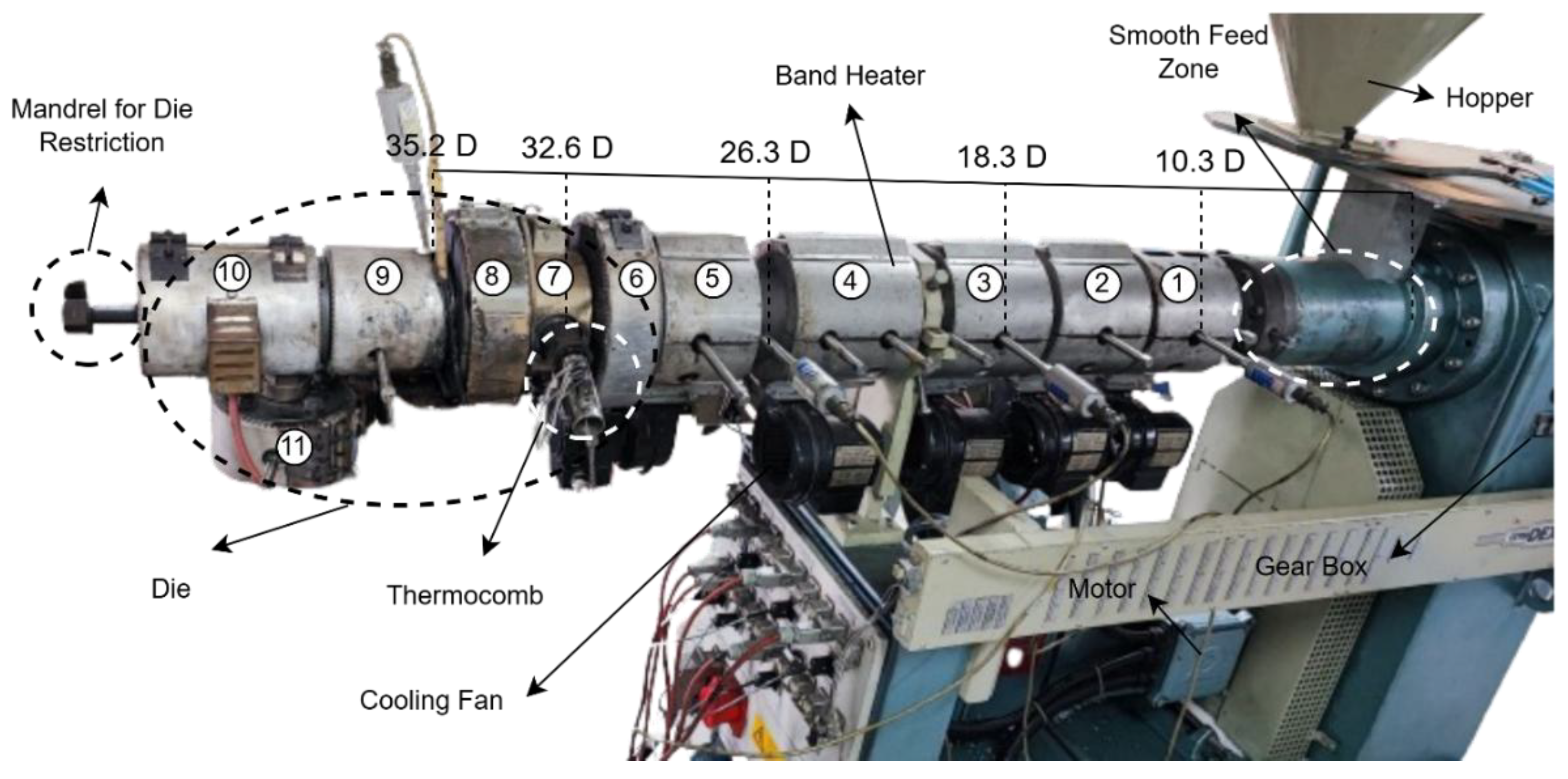
Figure 3.
Input variables.
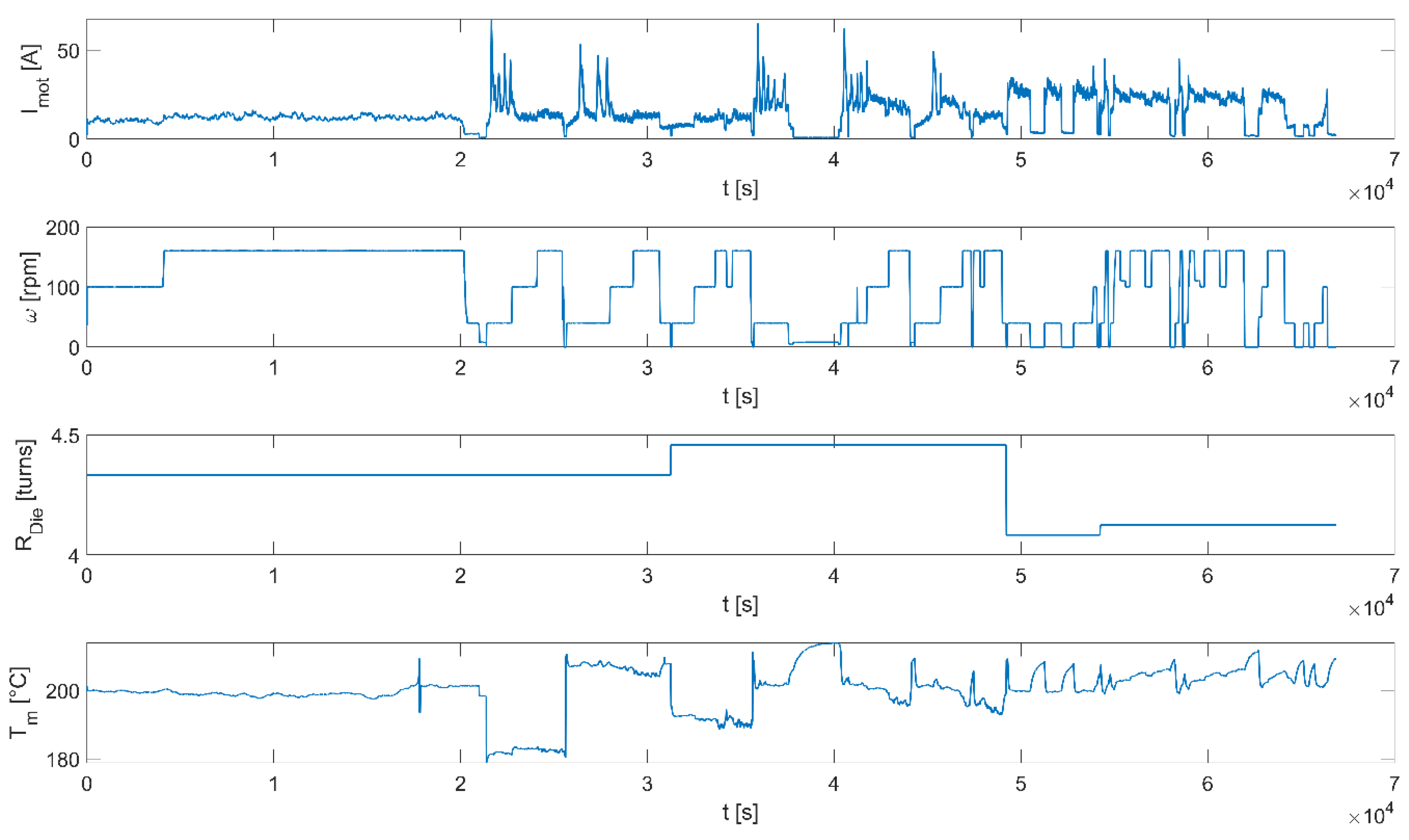
Figure 4.
Correlation between variables.

Figure 5.
Percentage of variance explained by each principal component.
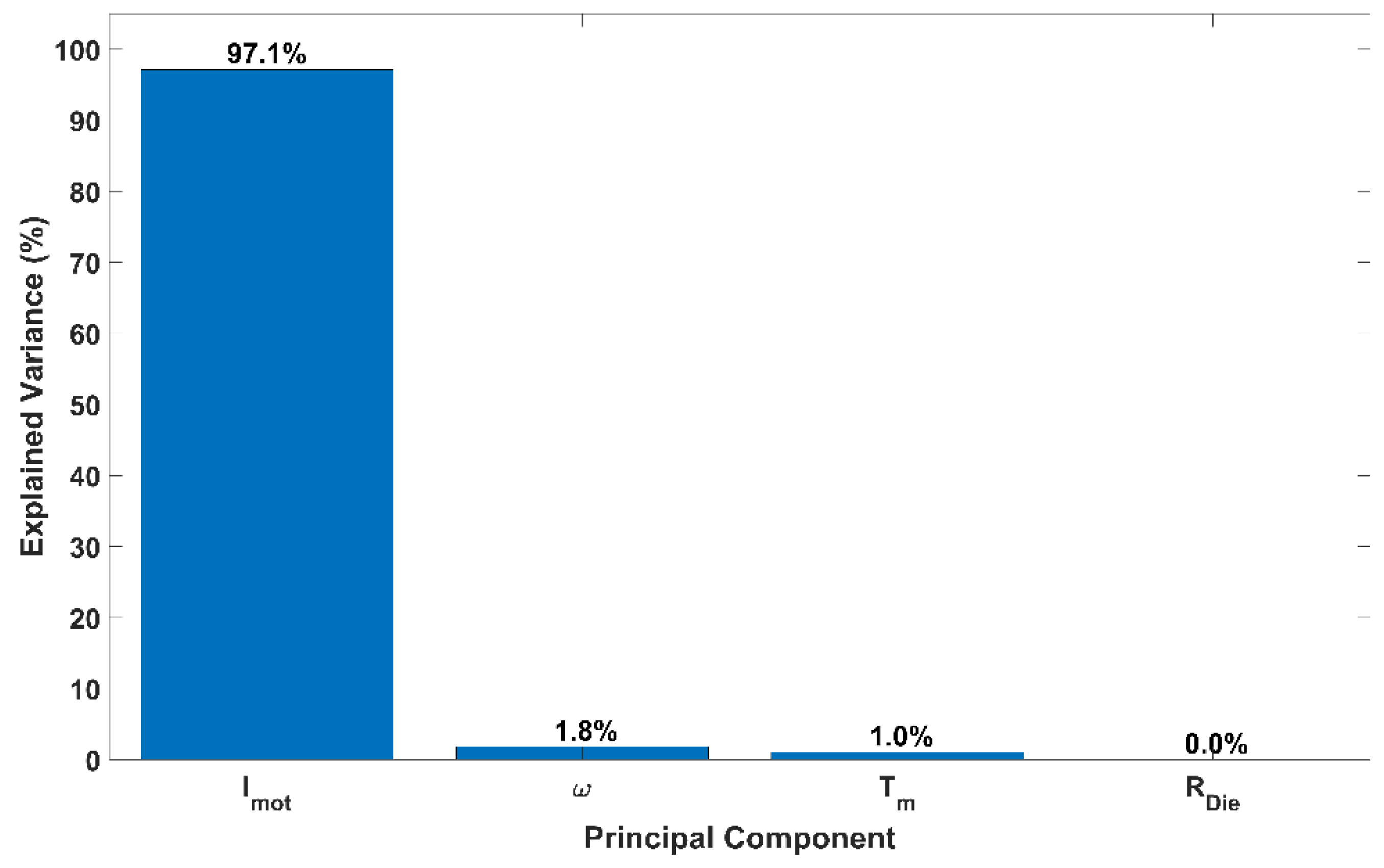
Figure 6.
Diagram of a 3-Hidden Layer Artificial Neural Network.
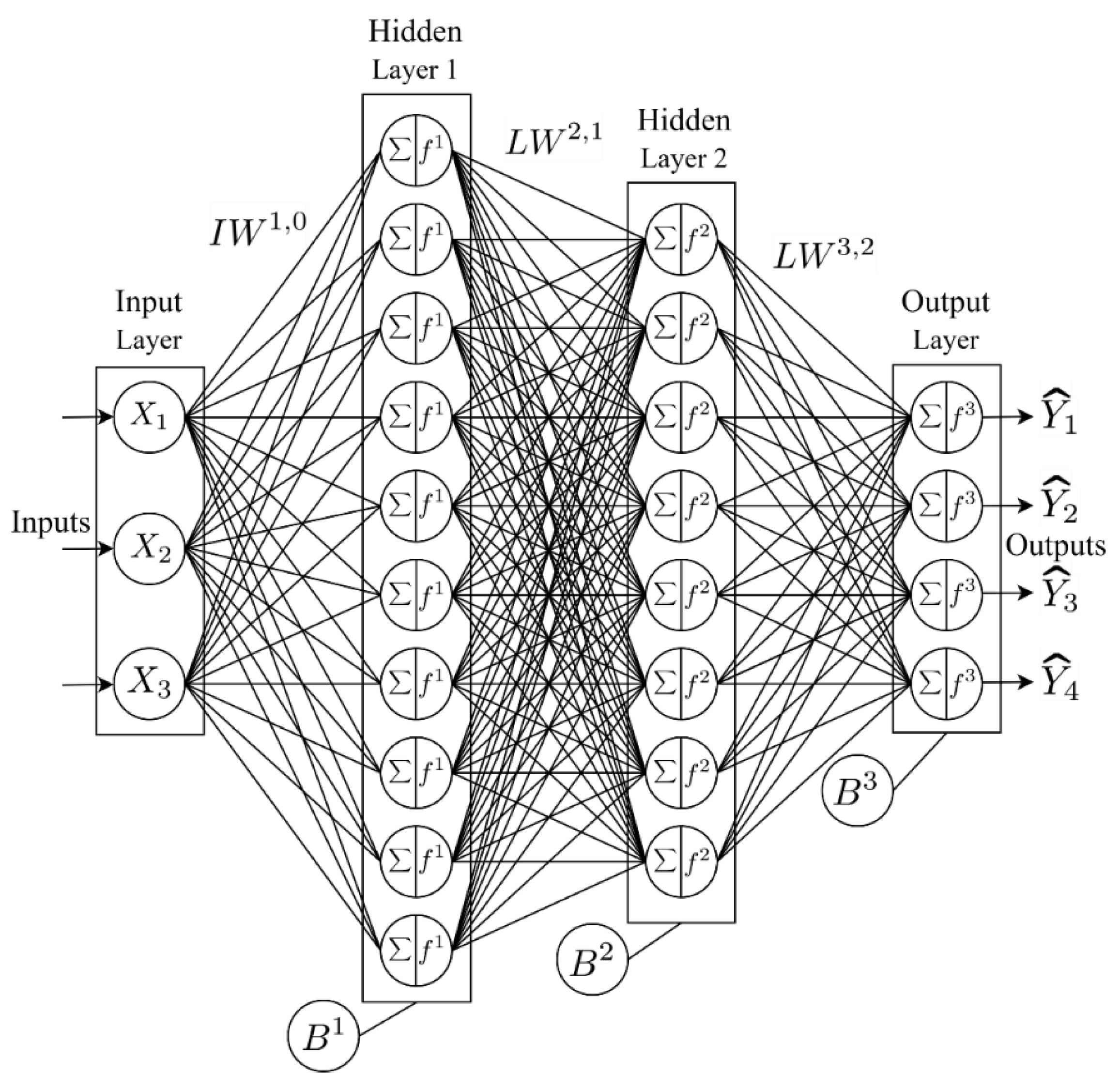
Figure 7.
Measured pressure profile data and pressure profile predictions with the Feedforward Artificial Neural Network.
Figure 7.
Measured pressure profile data and pressure profile predictions with the Feedforward Artificial Neural Network.
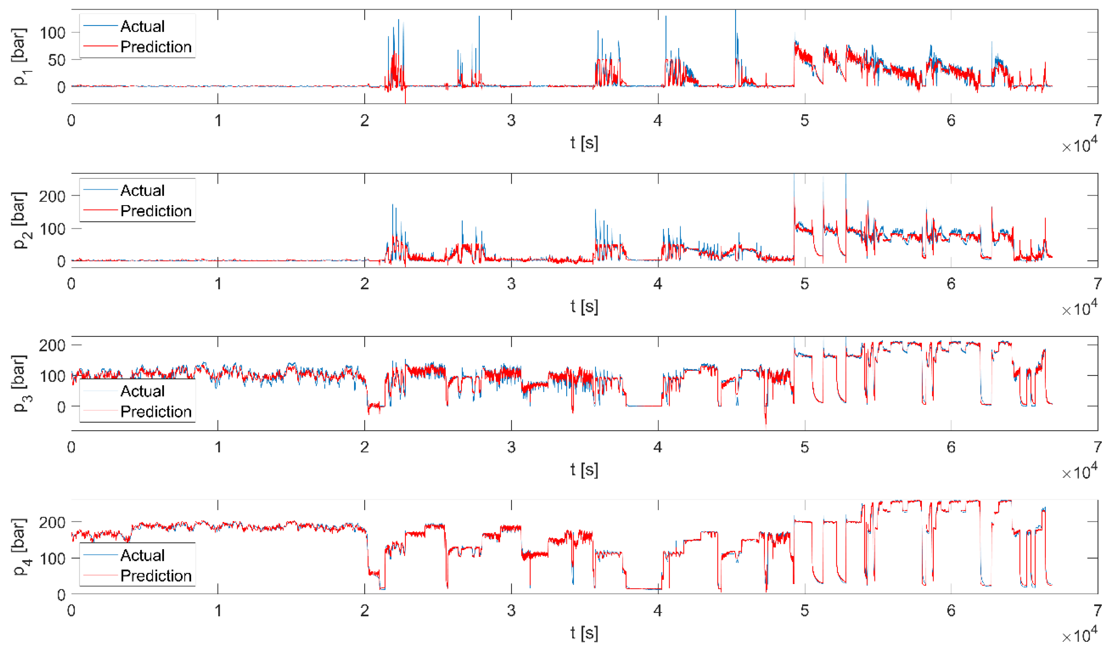
Table 1.
Barrel and die temperature sensors along the extruder.
| Heating Zone | 1 | 2 | 3 | 4 | 5 | 6 | 7 | 8 | 9 | 10 | 11 |
| 160 | 190 | 210 | 220 | 220 | 220 | 220 | 220 | 220 | 220 | 220 | |
| 10.3D | 14.3D | 18.3D | 24.3D | 28.3D | 30.5D | 32.3D | 35.8D | 41.8D | 50D | 54.2D |
Table 3.
Results of the Feedforward Artificial Neural Network Architectures.
| s | Metrics | ||||||||||||
| Train | Val | Test | All | Train | Val | Test | All | ||||||
| ,,, | 4 | 10 | 8 | 0.0075 | 0.0078 | 0.0078 | 0.0077 | 0.9894 | 0.9888 | 0.9889 | 0.9892 | 195 | 108 |
| , , , | 4 | 8 | 6 | 0.0092 | 0.0091 | 0.0093 | 0.0092 | 0.9869 | 0.9869 | 0.9868 | 0.9869 | 209 | 41 |
| , , | 3 | 10 | 8 | 0.0093 | 0.0097 | 0.0097 | 0.0096 | 0.9867 | 0.9861 | 0.9863 | 0.9866 | 224 | 80 |
| , , | 3 | 8 | 6 | 0.0099 | 0.0094 | 0.0099 | 0.0097 | 0.9858 | 0.9864 | 0.9860 | 0.9859 | 509 | 147 |
| , | 2 | 10 | 8 | 0.0261 | 0.0254 | 0.0255 | 0.0257 | 0.9623 | 0.9631 | 0.9634 | 0.9626 | 234 | 65 |
Disclaimer/Publisher’s Note: The statements, opinions and data contained in all publications are solely those of the individual author(s) and contributor(s) and not of MDPI and/or the editor(s). MDPI and/or the editor(s) disclaim responsibility for any injury to people or property resulting from any ideas, methods, instructions or products referred to in the content. |
© 2025 by the authors. Licensee MDPI, Basel, Switzerland. This article is an open access article distributed under the terms and conditions of the Creative Commons Attribution (CC BY) license (https://creativecommons.org/licenses/by/4.0/).
Copyright: This open access article is published under a Creative Commons CC BY 4.0 license, which permit the free download, distribution, and reuse, provided that the author and preprint are cited in any reuse.


