Defining a Satisfying Expected Value From Chosen Sequences of Bounded Functions Converging to Pathological Functions

1. Intro

Let $n\in \mathbb{N}$ and suppose function $f:A\subseteq {\mathbb{R}}^n\to \mathbb{R}$, where A and f are Borel. We want a satisfying average for all pathological f taking finite values only. The problem is the expected value of certain examples of f (§2.1,§2.2), w.r.t the Hausdorff measure in its dimension, is undefined (§2.3). To fix this, we take the expected value of a sequence of bounded functions converging to f (§2.3.2); however, depending on the sequence of bounded functions chosen, the expected value could be one of several values (thm. 1). Hence, we define a leading question (§3.1) which chooses sequences of bounded functions with the same satisfying and finite expected value, such the term “satisfying" is explained rigorously.

Note, the leading question ($\S$) was inspired by two problems (i.e., informal versions of thm. 2 and 5):

(1)

If $F\subset {\mathbb{R}}^A$ is the set of all $f\in {\mathbb{R}}^A$, where the expected value of f w.r.t the Hausdorff measure in its dimension is finite, then F is shy [13].

• If $F\subset {\mathbb{R}}^A$ is shy, we say “almost no" element of ${\mathbb{R}}^A$ lies in F (§2.4).

(2)

If $F\subset {\mathbb{R}}^A$ is the set of all $f\in {\mathbb{R}}^A$, where two sequences of bounded functions that converge to f have different expected values, then F is prevelant [13].

• If $F\subset {\mathbb{R}}^A$ is prevelant, we say “almost all" elements of ${\mathbb{R}}^A$ lies in F (§2.4).

In section $\S$, we clarify the leading question (§3.1) by applying the rigorous definitions of the leading question to specific examples (§5.2.1). We also define a “measure" (§5.3.1,§5.3.2) of the sequence of a bounded functions’ graphs. This is crucial for defining a satisfying expected value, where “measure" is defined by:

(1)

Covering each graph with minimal, pairwise disjoint sets of equal $\epsilon$ Hausdorff measure (§8.1)

(2)

Taking a sample point from each cover (§8.2)

(3)

Taking a “pathway of line segments" starting with sample point $x_0$ to the sample point with the smallest Euclidean distance from $x_0$ (i.e., when more than one point has the smallest Euclidean distance to $x_0$, take either of those points). Next, repeat this process until the pathway intersects with every sample point once (§8.3.1)

(4)

Taking the length of each line segments in the pathway and remove the outliers which are more than $C>0$ times the interquartile range of the length of each line segment as $\epsilon \to 0$ (§8.3.2),

(5)

Multiply the remaining lengths by a constant to get a probability distribution (§8.3.3)

(6)

Taking the entropy of the distribution (§8.3.4)

(7)

Taking the maximum entropy w.r.t all pathways (§8.3.5)

We give examples of how to apply the “measure" (§5.3.3-§5.3.5), then define the actual rate of expansion of a bounded functions’ graph (§5.4).

Finally, we answer the leading question in $\S$. Since the answer is complicated, is likely incorrect, and the leading question might not admit an unique expected value, it is best to keep refining the leading question (§3.1) instead of woring on an immediate solution.

2. Formalizing the Intro

Let $n\in \mathbb{N}$ and suppose function $f:A\subseteq {\mathbb{R}}^n\to \mathbb{R}$, where A and f are Borel. Let ${\dim }_{\mathrm{H}}(·)$ be the Hausdorff dimension, where ${\mathcal{H}}^{{\dim }_{\mathrm{H}}(·)}(·)$ is the Hausdorff measure in its dimension on the Borel $\sigma$-algebra.

We want an unique, satisfying average for each of the following functions (§2.1,§2.2) taking finite values only. We explain the method of averaging in later sections, starting from §2.3.1.

2.1. First Special Case of f

If the graph of f is G, we want an explicit f where:

(1)

The function f is everywhere surjective [1] (i.e., f is defined on a topological space where its’ restriction to any non-empty open subset is surjective).

(2)

${\mathcal{H}}^{{\dim }_{\mathrm{H}}\left(G\right)}\left(G\right)=0$

2.1.1. Potential Answer

If $A=\mathbb{R}$, using this post [3]:

Consider a Cantor set $C\subseteq [0,1]$ with Hausdorff dimension 0 [4]. Now consider a countable disjoint union ${\cup }_{m\in \mathbb{N}}{C}_m$ such that each $C_m$ is the image of C by some affine map and every open set $O\subseteq [0,1]$ contains $C_m$ for some m. Such a countable collection can be obtained by e.g. at letting $C_m$ be contained in the biggest connected component of $[0,1]\setminus (C_1\cup \cdots \cup C_{m-1})$ (with the center of $C_m$ being the middle point of the component).

Note that ${\cup }_m{C}_m$ has Hausdorff dimension 0, so $\left({\cup }_m{C}_m\right)\times [0,1]\subseteq {\mathbb{R}}^2$ has Hausdorff dimension one [2].

Now, let $g:[0,1]\to \mathbb{R}$ such that ${g|}_{C_m}$ is a bijection $C_m\to \mathbb{R}$ for all m (all of them can be constructed from a single bijection $C\to \mathbb{R}$, which can be obtained without choice, although it may be ugly to define) and outside ${\cup }_m{C}_m$ let g be defined by $g\left(x\right)=h\left(x\right)$, where $h:[0,1]\to \mathbb{R}$ has a graph with Hausdorff dimension 2 [14] (this doesn’t require choice either).

Then the function g has a graph with Hausdorff dimension 2 and is everywhere surjective, but its graph has Lebesgue measure 0 because it is a graph (so it admits uncountably many disjoint vertical translates).

Note, we can make the construction with union of $C_m$ rather explicit as follows. Split the binary expansion of x as strings of size with a power of two, say $x=0.1101000010\dots$ becomes $(s_0,s_1,s_2,\dots )=(1,10,1000,\dots )$. If this sequence eventually contains only strings of the form $0\cdots 0$ or $1\cdots 1$, say after $s_k$, then send it to $y={\sum }_{i>0}{ϵ}_i{2}^{-i}$, where $s_{k+i}={ϵ}_i\cdots {ϵ}_i$. Otherwise, send it to the explicit continuous function h given by the linked article [14]. This will give you something from $[0,1)\to [0,1)$

Finally, compose an explicit (reasonable) bijection from $[0,1)$ to $\mathbb{R}$. In your case, the construction can be easily adapted so that the $[0,1]$ or $[0,1)$ target space is actually $(0,1)$, then compose with $t\mapsto (1-2x)/(x^2-x)$.

In case we cannot obtain a unique, satisfying average $\left(\S \right)$ from $\S$, consider the following:

2.2. Second Special Case of f

Suppose, we define $A=\mathbb{Q}$, where $f:A\to \mathbb{R}$, such that:

$$f\left(x\right)=\left\{\begin{array}{cc}1\hfill & x\in \left\{(2s+1)/\left(2t\right):s\in \mathbb{Z},t\in \mathbb{N},t\ne 0\right\}\hfill \\ 0\hfill & x\notin \left\{(2s+1)/\left(2t\right):s\in \mathbb{Z},t\in \mathbb{N},t\ne 0\right\}\hfill \end{array}\right.$$

(1)

In the next section, we state why we want $\S$ and §2.2.

2.3. Attempting to Analyze/Average f

Suppose, the expected value of f w.r.t the Hausdorff measure in its dimension is:

$$\mathbb{E}\left[f\right]={\displaystyle \frac{1}{{\mathcal{H}}^{{\dim }_{\mathrm{H}}\left(A\right)}\left(A\right)}}{\int }_{A}fd{\mathcal{H}}^{{\dim }_{\mathrm{H}}\left(A\right)}$$

(2)

Then, using $\S$, the integral of f w.r.t the Hausdorff measure in its dimension is undefined: i.e., the graph of f has Hausdorff dimension 2 with a zero 2-d Hausdorff measure (§2.1.1). Hence, $\mathbb{E}\left[f\right]$ is undefined.

Moreover, obseve that in $\S$, f is nowhere continuous and defined on a countably infinite set, which means depending on the enumeration of A or the sequence ${\left\{a_r\right\}}_{r=1}^{\infty }$, where the expected value of f (when it exists) is:

$$\mathbb{E}\left[f\right]=\underset{t\to \infty }{lim}{\displaystyle \frac{f\left(a_1\right)+f\left(a_2\right)+···+f\left(a_t\right)}{t}}$$

(3)

the expected value $\mathbb{E}\left[f\right]$ is any number from $inff$ to $supf$. Hence, we need a specific enumeration that gives a unique, satisfying, and finite expected value, generalizing this process to nowhere continuous functions defined on uncountable domains.

Thus, we want the “expected value of chosen sequences of bounded functions converging to f with the same satisfying and finite expected value" which we describe rigorously in later sections; however, consider the following definitions beginning with §2.3.1:

2.3.1. Definition of Sequences of Functions Converging to f

Let $n\in \mathbb{N}$ and suppose function $f:A\subseteq {\mathbb{R}}^n\to \mathbb{R}$, where A and f are Borel.

The sequence of functions ${\left(f_r\right)}_{r\in \mathbb{N}}$, where $f_r:A_r\to \mathbb{R}$and${\left(A_r\right)}_{r\in \mathbb{N}}$ is a sequence of sets, converges to f when:

For any $x\in A$, there exists a sequence $\mathbf{x}\in A_r$s.t.$\mathbf{x}\to (x_1,···,x_n)$ and $f_r\left(\mathbf{x}\right)\to f(x_1,···,x_n)$.

This is equivelant to:

$$(f_r,A_r)\to (f,A)$$

2.3.2. Expected Value of Sequences of Functions Converging to f

Now, suppose:

• $(f_r,A_r)\to (f,A)$(§2.3.1)
• $\left|\right|·\left|\right|$ is the absolute value
• ${\dim }_{\mathrm{H}}(·)$ be the Hausdorff dimension
• ${\mathcal{H}}^{{\dim }_{\mathrm{H}}(·)}(·)$ is the Hausdorff measure in its dimension on the Borel $\sigma$-algebra
• the integral is defined, w.r.t the Hausdorff measure in its dimension

The expected value of ${\left(f_r\right)}_{r\in \mathbb{N}}$ is a real number $\mathbb{E}\left[f_r\right]$, when the following is true:

$$\begin{array}{cc}\hfill & \forall (ϵ>0)\exists (N\in \mathbb{N})\forall (r\in \mathbb{N})\left(r\ge N\Rightarrow \left|\left|{\displaystyle \frac{1}{{\mathcal{H}}^{{\dim }_{\mathrm{H}}\left(A_r\right)}\left(A_r\right)}}{\int }_{A_r}{f}_{r}d{\mathcal{H}}^{{\dim }_{\mathrm{H}}\left(A_r\right)}-\mathbb{E}\left[f_r\right]\right|\right|<ϵ\right)\hfill \end{array}$$

(4)

when no such $\mathbb{E}\left[f_r\right]$ exists, $\mathbb{E}\left[f_r\right]$ is infinite or undefined.

2.3.3. The Set of All Bounded Functions in a Function Space

Let $n\in \mathbb{N}$ and suppose the function $f:A\subseteq {\mathbb{R}}^n\to \mathbb{R}$, where A and f are Borel. Then, we define the following:

$\mathbf{B}(·)$ is the set of all bounded Borel functions in a function space

For example, $\mathbf{B}\left({\mathbb{R}}^A\right)$ is the set of all bounded Borel functions in ${\mathbb{R}}^A$ and $\mathbf{B}\left(2^{{\mathbb{R}}^n}\right)$ is the set of all bounded Borel subsets of ${\mathbb{R}}^n$. Note, however:

Theorem 1. 

For all $r,v\in \mathbb{N}$, suppose $f_r,g_v\in \mathbf{B}\left({\mathbb{R}}^A\right)$ and $A_r,B_v\in \mathbf{B}\left(2^{{\mathbb{R}}^n}\right)$. There exists a $f\in {\mathbb{R}}^A$, where $(f_r,A_r),(g_v,B_v)\to (f,A)$ and $\mathbb{E}\left[f_r\right]\ne \mathbb{E}\left[g_v\right]$($\S$2.3.2)

For example, the expected values of the sequences of bounded functions converging to f (§2.3.1, §2.3.2) in $\S$ and $\S$ satisfy thm. 1. For simplicity, we illustrate this with $\S$.

2.3.4. Example Illustrating Theorem 1

For the second case of Borel $f:A\subseteq {\mathbb{R}}^n\to \mathbb{R}$ (§2.2), where $A=\mathbb{Q}$, and:

$$f\left(x\right)=\left\{\begin{array}{cc}1\hfill & x\in \left\{(2s+1)/\left(2t\right):s\in \mathbb{Z},t\in \mathbb{N},t\ne 0\right\}\hfill \\ 0\hfill & x\notin \left\{(2s+1)/\left(2t\right):s\in \mathbb{Z},t\in \mathbb{N},t\ne 0\right\}\hfill \end{array}\right.$$

(5)

suppose:

$${\left(A_r\right)}_{r\in \mathbb{N}}={\left(\left\{c/r!:c\in \mathbb{Z},-r·r!\le c\le r·r!\right\}\right)}_{r\in \mathbb{N}}$$

and

$${\left(B_v\right)}_{v\in \mathbb{N}}=\left(\left\{c/d:c\in \mathbb{Z},d\in \mathbb{N},d\le v,-d·v\le c\le d·v\right\}\right)$$

where for $f_r:A_r\to \mathbb{R}$,

$$f_r\left(x\right)=f\left(x\right)\mathrm{for}\mathrm{all}x\in A_r$$

(6)

and for $g_v:B_v\to \mathbb{R}$

$$g_v\left(x\right)=f\left(x\right)\mathrm{for}\mathrm{all}x\in B_v$$

(7)

Note, $f_r$ and $g_v$ are bounded since f is bounded. Also, the set-theoretic limit of ${\left(A_r\right)}_{r\in \mathbb{N}}$ and ${\left(B_v\right)}_{r\in \mathbb{N}}$ is $A=\mathbb{Q}$: i.e.,

$$\begin{array}{c}\underset{r\to \infty }{lim\; sup}{A}_r=\bigcap _{r\ge 1}\bigcup _{q\ge r}{A}_q\\ \underset{r\to \infty }{lim\; inf}{A}_r=\bigcup _{r\ge 1}\bigcap _{q\ge r}{A}_q\end{array}$$

where:

$$\underset{r\to \infty }{lim\; sup}{A}_r=\underset{r\to \infty }{lim\; inf}{A}_r=A=\mathbb{Q}$$

$$\underset{v\to \infty }{lim\; sup}{B}_v=\underset{v\to \infty }{lim\; inf}{B}_v=A=\mathbb{Q}$$

(We aren’t sure how to prove the set-theoretic limits; however, a mathematician specializing in rational numbers and limits should be able to check.)

Hence, $(f_r,A_r),(g_v,B_v)\to (f,A)$ (thm. 1).

Now, suppose we want to average $f_r$ and $g_v$, which we denote $\mathbb{E}\left[f_r\right]$ and $\mathbb{E}\left[g_v\right]$. Note, this is the same as computing the following (i.e., the cardinality is $|·|$ and the absolute value is $\left|\right|·\left|\right|$):

$$\begin{array}{cc}\hfill & \forall (ϵ>0)\exists (N\in \mathbb{N})\forall (r\in \mathbb{N})\left(r\ge N\Rightarrow \left|\left|{\displaystyle \frac{1}{|A_r|}}{\int }_{A_r}f\left(x\right)d{\mathcal{H}}^0-\mathbb{E}\left[f_r\right]\right|\right|<ϵ\right)\Rightarrow \hfill \\ \hfill & \forall (ϵ>0)\exists (N\in \mathbb{N})\forall (r\in \mathbb{N})\left(r\ge N\Rightarrow \left|\left|{\displaystyle \frac{1}{|A_r|}}\sum _{x\in A_r}f\left(x\right)-\mathbb{E}\left[f_r\right]\right|\right|<ϵ\right)\hfill \\ \hfill \end{array}$$

(8)

$$\begin{array}{cc}\hfill & \forall (ϵ>0)\exists (N\in \mathbb{N})\forall (v\in \mathbb{N})\left(v\ge N\Rightarrow \left|\left|{\displaystyle \frac{1}{|B_v|}}{\int }_{B_v}f\left(x\right)d{\mathcal{H}}^0-\mathbb{E}\left[g_v\right]\right|\right|<ϵ\right)\Rightarrow \hfill \\ \hfill & \forall (ϵ>0)\exists (N\in \mathbb{N})\forall (v\in \mathbb{N})\left(v\ge N\Rightarrow \left|\left|{\displaystyle \frac{1}{|B_v|}}\sum _{x\in B_v}f\left(x\right)-\mathbb{E}\left[g_v\right]\right|\right|<ϵ\right)\hfill \\ \hfill \end{array}$$

(9)

Hence, if we assume $\mathbb{E}\left[f_r\right]=1$ in eq. 8, using [9]:

The sum ${\sum }_{x\in A^{★}}f\left(x\right)$ counts the number of fractions with an even denominator and an odd numerator in set $A^{★}$, after canceling all possible factors of 2 in the fraction. Let us consider the first case. We can write:

$$\left|\left|1-|A_r{|}^{-1}\sum _{x\in A_r}f\left(x\right)\right|\right|=\left(|A_r|-\sum _{x\in A_r}f\left(x\right)\right)/|A_r|=H\left(r\right)/|A_r|$$

where $H\left(r\right)$ counts the fractions $x=c/r_k!$ in $A_r$ that are not counted in ${\sum }_{x\in A^{★}}f\left(x\right)$, i.e., for which $f\left(x\right)=0$. This is the case when the denominator is odd after the cancellation of the factors of 2, i.e., when the numerator c has a number of factors of 2 greater than or equal to that of $r!$, which we will denote by $V\left(r\right):=v_2(r!)$ a.k.a the 2-valuation of $r!$, $\mathrm{oeis}\text{:}\mathrm{A}11371\left(r\right)=r-O(ln(r\left)\right)$[11]. That means, c must be a multiple of $2^{V\left(r\right)}$. The number of such c with $-r·r!\le c\le r·r$ is simply the length of that inteval, equal to $|A_r|=2r(r!)+1$, divided by $2^{V\left(r\right)}$. Thus,

$$\left|\left|1-|A_r{|}^{-1}\sum _{x\in A_r}f\left(x\right)\right|\right|=\left[\right|A_r|/2^{V\left(r\right)}]/|A_r|\sim 1/2^{V\left(r\right)}=1/2^{n-O(logn)}$$

This obviously tends to zero, proving $\mathbb{E}\left[f_r\right]=1$

Last, we need to show $\mathbb{E}\left[g_v\right]=1/3$, where $\mathbb{E}\left[f_r\right]\ne \mathbb{E}\left[g_v\right]$ proving theorem 1.

Concerning the second case [9], it is again simpler to consider the complementary set of $x\in B_v$ such that the denominator is odd when all possible factors of 2 are canceled. We can see that for $v=2p-1$, and these obviously include all those we had for smaller v. The “new" elements in $B_v$ with $v=2p-1$ are those that have the denominator $d=2p-1$ when written in lowest terms. Their number is equal to the number of $\kappa <d$, $gcd(\kappa ,d)=1$, which is given by Euler’s $\varphi$ function. Since we also consider negative fractions, we have to multiply this by 2. Including $x=0$, we have $G\left(v\right)=|\left\{x\in B_v|f\left(x\right)=0\right\}|=1+2{\sum }_{0\le \kappa \le v/2}\varphi (2\kappa +1)$. There is no simple explicit expression for this (cf. oeis:A99957 [12]), but we know that $G\left(v\right)=1+2·\mathrm{A}99957(v/2)\sim 2·8{(v/2)}^2/{\pi }^2=4v^2/{\pi }^2$ [12]. On the other hand, the total number of all elements of $B_v$ is $|B_v|=1+2{\sum }_{1\le \kappa \le v}\varphi \left(\kappa \right)$, since each time we increase v by 1, we have the additional fractions with the new denominator $d=v$ and the numerators are coprime with d, again with the sign + or −. From oeis:A002088 [10] we know that ${\sum }_{1\le \kappa \le v}\varphi \left(\kappa \right)=3v^2/{\pi }^2+O(vlogv)$, so $|B_v|\sim 6v^2/{\pi }^2$, which finally gives $|B_v{|}^{-1}{\sum }_{x\in B_v}f\left(x\right)=\left(\right|B_v|-G\left(v\right))/|B_v|\sim (6-4)/6=1/3$ as desired.

Hence, $\mathbb{E}\left[g_v\right]=1/3$ and $\mathbb{E}\left[f_r\right]\ne \mathbb{E}\left[g_v\right]$ proving thm.1.

Thus, consider:

2.4. Definition of Prevalent and Shy Sets

A Borel set $E\subset X$ is said to be prevalent if there exists a Borel measure $\mu$ on X such that:

(1)

$0<\mu \left(C\right)<\infty$ for some compact subset C of X, and

(2)

the set $E+x$ has full $\mu$-measure (that is, the complement of $E+x$ has measure zero) for all $x\in X$.

More generally, a subset F of X is prevalent if F contains a prevalent Borel Set.

Moreover:

• The complement of a prevelant set is a shy set.

Hence:

• If $F\subset X$ is prevelant, we say “almost every" element of X lies in F.
• If $F\subset X$ is shy, we say “almost no" element of X lies in F.

2.5. Motivation for Averaging $\S$ and $\S$

If $\mathbb{E}\left[f\right]$ is the expected value of f, w.r.t the Hausdorff measure in its dimension,

$$\mathbb{E}\left[f\right]={\displaystyle \frac{1}{{\mathcal{H}}^{{\dim }_{\mathrm{H}}\left(A\right)}\left(A\right)}}{\int }_{A}fd{\mathcal{H}}^{{\dim }_{\mathrm{H}}\left(A\right)}$$

(10)

Consider the following problems:

Theorem 2. 

If $F\subset {\mathbb{R}}^A$ is the set of all $f\in {\mathbb{R}}^A$, where $\mathbb{E}\left[f\right]$ is finite, then F is shy $\left(\S \right)$.

Note 3 

(Proof theorem 2 is true). We follow the argument presented in Example 3.6 of this paper [13], take $X:=L^0\left(A\right)$ (measurable functions over A), let P denote the one-dimensional subspace of A consisting of constant functions (assuming the Lebesgue measure on A) and let $F:=L^0\left(A\right)\setminus L^1\left(A\right)$ (measurable functions over A without finite integral). Let ${\lambda }_P$ denote the Lebesgue measure over P, for any fixed $f\in F$:

$${\lambda }_P\left(\left\{\alpha \in \mathbb{R}|{\int }_A(f+\alpha )d\mu <\infty \right\}\right)=0$$

Meaning P is a one-dimensional, so f is a 1-prevalent set.

Note 4 

(Way of Approaching Theorem 2). For all $r\in \mathbb{N}$, suppose that $f_r\in \mathbf{B}\left({\mathbb{R}}^A\right)$ and $A_r\in \mathbf{B}\left(2^{{\mathbb{R}}^n}\right)$. If $F\subset {\mathbb{R}}^A$ is the set of all $f\in {\mathbb{R}}^A$, where there exists $r\in \mathbb{N}$ such that $(f_r,A_r)\to (f,A)$ and $\mathbb{E}\left[f_r\right]$ is finite ($\S$2.3.2), then F should be prevalent ($\S$2.4) or neither prevalent nor shy ($\S$2.4).

Theorem 5. 

For all $r,v\in \mathbb{N}$, suppose $f_r,g_v\in \mathbf{B}\left({\mathbb{R}}^A\right)$ and $A_r,B_v\in \mathbf{B}\left(2^{{\mathbb{R}}^n}\right)$. When $F\subset {\mathbb{R}}^A$ is the set of all $f\in {\mathbb{R}}^A$, where $(f_r,A_r),(g_v,B_v)\to (f,A)$ and $\mathbb{E}\left[f_r\right]\ne \mathbb{E}\left[g_v\right]$, then F is prevalent ($\S$2.4).

Note 6 

(Possible method to proving theorem 5 true). For all $r,v\in \mathbb{N}$, suppose $f_r,g_v\in \mathbf{B}\left({\mathbb{R}}^A\right)$ and $A_r,B_v\in \mathbf{B}\left(2^{{\mathbb{R}}^n}\right)$. Therefore, suppose $Q\subset {\mathbb{R}}^A$ is the set of all $f\in {\mathbb{R}}^A$ whose lines of symmetry intersect at one point, where if $(f_r,A_r),(g_v,B_v)\to (f,A)$, then note $\mathbb{E}\left[f_r\right]=\mathbb{E}\left[g_v\right]$. In addition, $Q^{\prime }\subset {\mathbb{R}}^A$ is the set of symmetric $f\in {\mathbb{R}}^A$ which clearly forms a shy subset of ${\mathbb{R}}^A$. Since $Q\subset Q^{\prime }$, we have proven that Q is also shy (i.e., a subset of a shy set is also shy). Since the complement of the shy set Q is prevalent, $F={\mathbb{R}}^A\setminus Q$ is prevalent, such that for all $f\in F$, where $(f_r,A_r),(g_v,A_v)\to (f,A)$ and $\mathbb{E}\left[f_r\right]\ne \mathbb{E}\left[g_v\right]$. If this is correct, we have partially proven thm. 5.

Note 7 

(Way of Approaching Theorem 5). Suppose $\mathcal{B}\subset \mathbf{B}\left({\mathbb{R}}^A\right)$ and $\mathcal{B}\subset \mathbf{B}\left(2^{{\mathbb{R}}^n}\right)$ are arbitrary sets, such that for all $r\in \mathbb{N}$, $f_r\in \mathcal{B}$ and $A_r\in \mathcal{B}$. If $F\subset {\mathbb{R}}^A$ is the set of all $f\in {\mathbb{R}}^A$, where $(f_r,A_r)\to (f,A)$ and $\mathbb{E}\left[f_r\right]$ is unique, then F should be prevelant ($\S$2.4).

Since thm. 2 and 5 are true, we need to solve both theorems at once with the following:

2.5.1. Approach

Suppose $\mathcal{B}\subset \mathbf{B}\left({\mathbb{R}}^A\right)$ and $\mathcal{B}\subset \mathbf{B}\left(2^{{\mathbb{R}}^n}\right)$ are arbitrary sets, such that for all $r\in \mathbb{N}$, $f_r\in \mathcal{B}$ and $A_r\in \mathcal{B}$. If $F\subset {\mathbb{R}}^A$ is the collection of all $f\in {\mathbb{R}}^A$, where $(f_r,A_r)\to (f,A)$ and $\mathbb{E}\left[f_r\right]$ is unique, satisfying ($\S$3) and finite, then F should be:

(1)

a prevalent (§2.4) subset of ${\mathbb{R}}^A$

(2)

If not prevalent (§2.4) then neither prevalent (§2.4) nor shy (§2.4) subset of ${\mathbb{R}}^A$.

3. Attempt to Define “Satisfying” in The Approach of §2.5.1

3.1. Leading Question

To define satisfying in the blockquote of the §2.5.1, we ask the leading question...

Suppose, there exists arbitrary sets $\mathcal{B}\subset \mathbf{B}\left({\mathbb{R}}^A\right)$ and $\mathcal{B}\subset \mathbf{B}\left(2^{{\mathbb{R}}^n}\right)$, where for all $r,v\in \mathbb{N}$:

(A)

$f_r^{★}\in \mathcal{B}$ and $A_r^{★}\in \mathcal{B}$

(B)

$f_v^{★★}\in \mathbf{B}\left({\mathbb{R}}^A\right)\setminus \mathcal{B}$ and $A_v^{★★}\in \mathbf{B}\left(2^{{\mathbb{R}}^n}\right)\setminus \mathcal{B}$

(C)

${\left(G_r^{★}\right)}_{r\in \mathbb{N}}={\left(\mathrm{graph}\left(f_r^{★}\right)\right)}_{r\in \mathbb{N}}$ is the sequence of the graph of each $f_r^{★}$

(D)

□ is the logical symbol for “it’s necessary"

(E)

C is the chosen center point of ${\mathbb{R}}^{n+1}$ (e.g., the origin)

(F)

E is the fixed, expected rate of expansion of ${\left(G_r^{★}\right)}_{r\in \mathbb{N}}$ w.r.t center point C: e.g., $E=1$ (§3.1.C, §3.1.E)

(G)

$\mathcal{E}(C,G_r^{★})$ is the actual rate of expansion of ${\left(G_r^{★}\right)}_{r\in \mathbb{N}}$ w.r.t center point C ($\S$3.1.C, §3.1.E, $\S$5.4)

Does there exist an unique choice function, which chooses an unique set $\mathcal{B}\subset \mathbf{B}\left({\mathbb{R}}^A\right)$ and $\mathcal{B}\subset \mathbf{B}\left(2^{{\mathbb{R}}^n}\right)$, where for all $r\in \mathbb{N}$, $f_r^{★}\in \mathcal{B}$ and $A_r^{★}\in \mathcal{B}$, such that:

(1)

$(f_r^{★},A_r^{★})\to (f,A)$ (§2.3.1)

(2)

For all $v\in \mathbb{N}$, where $f_v^{★★}\in \mathbf{B}\left({\mathbb{R}}^A\right)\setminus \mathcal{B}$ and $A_v^{★★}\in \mathbf{B}\left(2^{{\mathbb{R}}^n}\right)\setminus \mathcal{B}$, the “measure" (§5.3.1, §5.3.2) of $G_r^{★}=\mathrm{graph}\left(f_r^{★}\right)$ (§3.1.C) must increase at a rate linear or superlinear to that of $G_v^{★★}=\mathrm{graph}\left(f_v^{★★}\right)$ (§3.1.C)

(3)

$\mathbb{E}\left[f_r^{★}\right]$ is unique and finite (§2.3.2)

(4)

For some $f_r^{★}\in \mathcal{B}$ and $A_r^{★}\in \mathcal{B}$ satisfying (1), (2) and (3), when f is unbounded (i.e, skip (4) when f is bounded), for all sets ${\mathcal{B}}^{\prime }\subset \mathbf{B}\left({\mathbb{R}}^A\right)$ and ${\mathcal{B}}^{\prime }\subset \mathbf{B}\left(2^{{\mathbb{R}}^n}\right)$, where $★\mapsto ★★★$, $r\mapsto s$, $\mathcal{B}\mapsto {\mathcal{B}}^{\prime }$, and $\mathcal{B}\mapsto {\mathcal{B}}^{\prime }$ in (1), (2) and (3), s.t.$\neg \square (\mathbb{E}\left[f_r^{★}\right]=\mathbb{E}\left[f_s^{★★★}\right])$ (§2.3.1, §2.3.2, §3.1.D), for every $s\in \mathbb{N}$, where both $f_s^{★★★}\in {\mathcal{B}}^{\prime }$ and $A_s^{★★★}\in {\mathcal{B}}^{\prime }$ satisfy (1), (2) and (3):

• If the absolute value is $\left|\right|·\left|\right|$ and the $(n+1)$-th coordinate of C (§3.1.E) is $x_{n+1}$, $\left|\right|\mathbb{E}\left[f_r^{★}\right]-x_{n+1}\left|\right|\le \left|\right|\mathbb{E}\left[f_s^{★★★}\right]-x_{n+1}\left|\right|$ (§2.3.1, §2.3.2)
• If $r\in \mathbb{N}$, then for any linear $s_1:\mathbb{N}\to \mathbb{N}$, where $s=s_1\left(r\right)$ and the Big-O notation is $\mathcal{O}$, there exists a function $K:\mathbb{R}\to \mathbb{R}$, where (§3.1.E-F):

  $$\begin{array}{cc}\hfill \left|\right|\mathcal{E}(C,G_r^{★})-E\left|\right|=& \mathcal{O}\left(K\right(\left|\right|\mathcal{E}(C,G_s^{★★★})-E\left|\right|\left)\right)\hfill \\ \hfill =& \mathcal{O}\left(K\right(\left|\right|\mathcal{E}(C,G_{s_1\left(r\right)}^{★★★})-E\left|\right|\left)\right)\hfill \end{array}$$
  such that:

  $$0\le \underset{x\to +\infty }{lim}K\left(x\right)/x<+\infty$$
  In simpler terms, “the rate of divergence" of $\left|\right|\mathcal{E}(C,G_r^{★})-E\left|\right|$ (§3.1.D-E) is less than or equal to “the rate of divergence" of $\left|\right|\mathcal{E}(C,G_s^{★★★})-E\left|\right|$ (§3.1.D-E).

(5)

When set $F\subset {\mathbb{R}}^A$ is the set of all $f\in {\mathbb{R}}^A$, where a choice function chooses a collection $\mathcal{B}\subset \mathbf{B}\left({\mathbb{R}}^A\right)$ and $\mathcal{B}\subset \mathbf{B}\left(2^{{\mathbb{R}}^n}\right)$, such that $f_r^{★}\in \mathcal{B}$ and $A_r^{★}\in \mathcal{B}$ satisfy (1), (2), (3) and (4), then F should be:

(a)

a prevelant (§2.4) subset of ${\mathbb{R}}^A$

(b)

If not (0a) then neither a prevelant (§2.4) nor shy (§2.4) subset of ${\mathbb{R}}^A$

(6)

Out of all choice functions which satisfy (3.1), (3.1), (3.1), (3.1) and (3.1), we choose the one with the simplest form, meaning for each choice function fully expanded, we take the one with the fewest variables/numbers?

(In case this is unclear, see §5.)

We are convinced $\mathbb{E}\left[f_r^{★}\right]$ in (§3.1 crit. 3.1) isn’t unique nor satisfying enough to answer the approach of §2.5.1. Still, adjustments are possible by changing the criteria or by adding new criteria to the question.

4. Question Regarding My Work

Most don’t have time to address everything in my research, hence I ask the following:

Is there a research paper which already solves the ideas I’m woring on? (Non-published papers, such as mine [7], don’t count.)

5. Clarifying §3

See §3.1 once reading §5, and consider the following:

Is there a simpler version of the definitions below?

5.1. Example of Sequences of Bounded Functions Converging to f (§2.3.1)

The sequence of bounded functions ${\left(f_r\right)}_{r\in \mathbb{N}}$, where $f_r:A_r\to \mathbb{R}$ and ${\left(A_r\right)}_{r\in \mathbb{N}}$ is a sequence of bounded sets, converges to Borel $f:A\subseteq {\mathbb{R}}^n\to \mathbb{R}$ when:

For any $x\in A$ there exists a sequence $\mathbf{x}\in A_r$ s.t. $\mathbf{x}\to (x_1,···,x_n)$ and $f_r\left(\mathbf{x}\right)\to f(x_1,···,x_n)$ (see [5] for info).

Example 0.1

(Example of §2.3.1). If $A=\mathbb{R}$ and $f:A\to \mathbb{R}$, where $f\left(x\right)=1/x$, then an example of ${\left(f_r\right)}_{r\in \mathbb{N}}$, such that $f_r:A_r\to \mathbb{R}$ is:

(1)

${\left(A_r\right)}_{r\in \mathbb{N}}={([-r,-1/r]\cup [1/r,r])}_{r\in \mathbb{N}}$

(2)

$f_r\left(x\right)=1/x$ for $x\in A_r$

Example 0.2

(More Complex Example). If $A=\mathbb{R}$ and $f:A\to \mathbb{R}$, where $f\left(x\right)=x$, then an example of ${\left(f_r\right)}_{r\in \mathbb{N}}$, such that $f_r:A_r\to \mathbb{R}$ is:

(1)

${\left(A_r\right)}_{r\in \mathbb{N}}={\left([-r,r]\right)}_{r\in \mathbb{N}}$

(2)

$f_r\left(x\right)=x+(1/r)sin\left(x\right)$ for $x\in A_r$

5.2. Expected Value of Bounded Sequence of Functions

For some $k\in S$ (§2.3.1), the expected value of ${\left(f_r\right)}_{r\in \mathbb{N}}$ is a real number $\mathbb{E}\left[f_r\right]$, when the following is true:

$$\begin{array}{cc}\hfill & \forall (ϵ>0)\exists (N\in \mathbb{N})\forall (r\in \mathbb{N})\left(r\ge N\Rightarrow \left|\left|{\displaystyle \frac{1}{{\mathcal{H}}^{{\dim }_{\mathrm{H}}\left(A_r\right)}\left(A_r\right)}}{\int }_{A_r}{f}_{r}d{\mathcal{H}}^{{\dim }_{\mathrm{H}}\left(A_r\right)}-\mathbb{E}\left[f_r\right]\right|\right|<ϵ\right)\hfill \end{array}$$

(11)

otherwise when no such $\mathbb{E}\left[f_r\right]$ exists, $\mathbb{E}\left[f_r\right]$ is infinite or undefined.

5.2.1. Example

Using example 0.1, when ${\left(f_r\right)}_{r\in \mathbb{N}}={\left(\left\{(x,1/x):x\in [-r,-1/r]\cup [1/r,r]\right\}\right)}_{r\in \mathbb{N}}$ where:

(1)

${\left(A_r\right)}_{r\in \mathbb{N}}={\left([-r,-1/r]\cup [1/r,r]\right)}_{r\in \mathbb{N}}$

(2)

$f_r\left(x\right)=1/x$ for $x\in A_r$

If we assume $\mathbb{E}\left[f_r\right]=0$:

$$\begin{array}{cc}\hfill & \forall (ϵ>0)\exists (N\in \mathbb{N})\forall (r\in \mathbb{N})\left(r\ge N\Rightarrow \left|\left|{\displaystyle \frac{1}{{\mathcal{H}}^{{\dim }_{\mathrm{H}}\left(A_r\right)}\left(A_r\right)}}{\int }_{A_r}{f}_{r}d{\mathcal{H}}^{{\dim }_{\mathrm{H}}\left(A_r\right)}-\mathbb{E}\left[f_r\right]\right|\right|<ϵ\right)=\hfill \end{array}$$

(12)

$$\begin{array}{cc}\hfill & \forall (ϵ>0)\exists (N\in \mathbb{N})\forall (r\in \mathbb{N})(r\ge N\Rightarrow \hfill \end{array}$$

(13)

$$\begin{array}{cc}\hfill & \left.\left|\left|{\displaystyle \frac{1}{{\mathcal{H}}^{{\dim }_{\mathrm{H}}([-r,-1/r]\cup [1/r,r])}([-r,-1/r]\cup [1/r,r])}}{\int }_{[-r,-1/r]\cup [1/r,r]}1/xd{\mathcal{H}}^{{\dim }_{\mathrm{H}}([-r,-1/r]\cup [1/r,r])}-0\right|\right|<ϵ\right)=\hfill \end{array}$$

(14)

$$\begin{array}{cc}\hfill & \forall (ϵ>0)\exists (N\in \mathbb{N})\forall (r\in \mathbb{N})\left(r\ge N\Rightarrow \left|\left|{\displaystyle \frac{1}{{\mathcal{H}}^1([-r,-1/r]\cup [1/r,r])}}{\int }_{[-r,-1/r]\cup [1/r,r]}1/xd{\mathcal{H}}^1\right|\right|<ϵ\right)=\hfill \end{array}$$

(15)

$$\begin{array}{cc}\hfill & \forall (ϵ>0)\exists (N\in \mathbb{N})\forall (r\in \mathbb{N})\left(r\ge N\Rightarrow \left|\left|{\displaystyle \frac{1}{(-1/r-(-r\left)\right)+(r-1/r)}}\left({\int }_{-r}^{-1/r}1/xdx+{\int }_{1/r}^{r}1/xdx\right)\right|\right|<ϵ\right)=\hfill \end{array}$$

(16)

$$\begin{array}{cc}\hfill & \forall (ϵ>0)\exists (N\in \mathbb{N})\forall (r\in \mathbb{N})\left(r\ge N\Rightarrow \left|\left|{\displaystyle \frac{1}{(r-1/r)+(-1/r+r)}}\left(ln\left(\right|\left|x\right|\left|\right)+C{|}_{-r}^{-1/r}+ln\left(\right|\left|x\right|\left|\right)+C{|}_{1/r}^r\right)\right|\right|<ϵ\right)=\hfill \end{array}$$

(17)

$$\begin{array}{cc}\hfill & \forall (ϵ>0)\exists (N\in \mathbb{N})\forall (r\in \mathbb{N})\left(r\ge N\Rightarrow \left|\left|{\displaystyle \frac{1}{(r-1/r)+(-1/r+r)}}\left(ln\left(\right||-r|\left|\right)-ln\left(\right||-1/r|\left|\right)+ln\left(\right|\left|r\right|\left|\right)-ln\left(\right||1/r|\left|\right)\right)\right|\right|<ϵ\right)=\hfill \end{array}$$

(18)

$$\begin{array}{cc}\hfill & \forall (ϵ>0)\exists (N\in \mathbb{N})\forall (r\in \mathbb{N})\left(r\ge N\Rightarrow \left|\left|{\displaystyle \frac{1}{2r-2/r}}·4ln\left(r\right)\right|\right|<ϵ\right)=\hfill \end{array}$$

(19)

To prove eq. 19 is true, recall:

$$\begin{array}{cc}\hfill & r\ll e^{r/2},e^{1/r}\ll e^r\hfill \end{array}$$

(20)

$$\begin{array}{cc}\hfill & r\ll e^{r/2},e^{1/\left(2r\right)}\ll e^{r/2}\hfill \end{array}$$

(21)

$$\begin{array}{cc}\hfill & r{e}^{1/\left(2r\right)}\ll e^{r/2}\hfill \end{array}$$

(22)

$$\begin{array}{cc}\hfill & r\ll e^{r/2}/e^{1/\left(2r\right)}\hfill \end{array}$$

(23)

$$\begin{array}{cc}\hfill & r\ll e^{r/2-1/\left(2r\right)}\hfill \end{array}$$

(24)

$$\begin{array}{cc}\hfill & ln\left(r\right)\ll r/2-1/\left(2r\right)\hfill \end{array}$$

(25)

$$\begin{array}{cc}\hfill & 4ln\left(r\right)\ll 2r-2/r\hfill \end{array}$$

(26)

Hence, for all $\epsilon >0$

$$\begin{array}{cc}\hfill & 4ln\left(r\right)<\epsilon (2r-2/r)\hfill \end{array}$$

(27)

$$\begin{array}{cc}\hfill & {\displaystyle \frac{4ln\left(r\right)}{2r-2/r}}<\epsilon \hfill \end{array}$$

(28)

$$\begin{array}{cc}\hfill & \left|\left|{\displaystyle \frac{4ln\left(r\right)}{2r-2/r}}\right|\right|<\epsilon \hfill \end{array}$$

(29)

Since eq. 19 is true, $\mathbb{E}\left[f_r\right]=0$. Note, if we simply took the average of f from $(-\infty ,\infty )$, using the improper integral, the expected value:

$$\begin{array}{cc}\hfill & \underset{(x_1,x_2,x_3,x_4)\to (-\infty ,0^{-},0+,+\infty )}{lim}{\displaystyle \frac{1}{(x_4-x_3)+(x_2-x_1)}}\left({\int }_{x_1}^{x_2}{\displaystyle \frac{1}{x}}dx+{\int }_{x_3}^{x_4}{\displaystyle \frac{1}{x}}dx\right)=\hfill \end{array}$$

(30)

$$\begin{array}{cc}\hfill & \underset{(x_1,x_2,x_3,x_4)\to (-\infty ,0^{-},0+,+\infty )}{lim}{\displaystyle \frac{1}{(x_4-x_3)+(x_2-x_1)}}\left(ln\left(\right|\left|x\right|\left|\right)+C{|}_{x_1}^{x_2}+ln\left(\right|\left|x\right|\left|\right)+C{|}_{x_3}^{x_4}\right)=\hfill \end{array}$$

(31)

$$\begin{array}{cc}\hfill & \underset{(x_1,x_2,x_3,x_4)\to (-\infty ,0^{-},0+,+\infty )}{lim}{\displaystyle \frac{1}{(x_4-x_3)+(x_2-x_1)}}\left(ln\left(\right||x_2\left|\right|)-ln\left(\right||x_1\left|\right|)+ln\left(\right||x_4\left|\right|)-ln\left(\right||x_3\left|\right|)\right)\hfill \end{array}$$

(32)

is $+\infty$ (when $x_2=1/x_1$, $x_3=1/x_4$, and $x_1=exp\left(x_4^2\right)$) or $-\infty$ (when $x_2=1/x_1$, $x_3=1/x_4$, and $x_4=-exp\left(x_1^2\right)$), making $\mathbb{E}\left[f\right]$ undefined. (However, using eq. 12-19, we get the $\mathbb{E}\left[f_r\right]=0$ instead of an undefined value.)

5.3. Defining the “Measure"

5.3.1. Preliminaries

We define the “measure" of ${\left(G_r^{★}\right)}_{r\in \mathbb{N}}$, in $\S$, which is the sequence of the graph of each $f_r^{★}$ (§2.3.1). To understand this “measure", continue reading.

(1)

For every $r\in \mathbb{N}$, “over-cover" $G_r^{★}$ with minimal, pairwise disjoint sets of equal ${\mathcal{H}}^{{\dim }_{\mathrm{H}}\left(G_r^{★}\right)}$ measure. (We denote the equal measures $\epsilon$, where the former sentence is defined $\mathbf{C}(\epsilon ,G_r^{★},\omega )$: i.e., $\omega \in {\Omega }_{\epsilon ,r}$ enumerates all collections of these sets covering $G_r^{★}$. In case this step is unclear, see §8.1.)

(2)

For every $\epsilon$, r and $\omega$, take a sample point from each set in $\mathbf{C}(\epsilon ,G_r^{★},\omega )$. The set of these points is “the sample" which we define $\mathcal{S}(\mathbf{C}(\epsilon ,G_r^{★},\omega ),\psi )$: i.e., $\psi \in {\Psi }_{\epsilon ,r,\omega }$ enumerates all possible samples of $\mathbf{C}(\epsilon ,G_r^{★},\omega )$. (If this is unclear, see §8.2.)

(3)

For every $\epsilon$, r, $\omega$ and $\psi$,

(a)

Take a “pathway” of line segments: we start with a line segment from arbitrary point $x_0$ of $\mathcal{S}(\mathbf{C}(\epsilon ,G_r^{★},\omega ),\psi )$ to the sample point with the smallest $(n+1)$-dimensional Euclidean distance to $x_0$ (i.e., when more than one sample point has the smallest $(n+1)$-dimensional Euclidean distance to $x_0$, take either of those points). Next, repeat this process until the “pathway” intersects with every sample point once. (In case this is unclear, see §8.3.1.)

(b)

Take the set of the length of all segments in (3a), except for lengths that are outliers (i.e., for any constant $C>0$, the outliers are more than C times the interquartile range of the length of all line segments as $\epsilon \to 0$). Define this $\mathcal{L}(x_0,\mathcal{S}(\mathbf{C}(\epsilon ,G_r^{★},\omega ),\psi ))$. (If this is unclear, see §8.3.2.)

(c)

Multiply remaining lengths in the pathway by a constant so they add up to one (i.e., a probability distribution). This will be denoted $\mathbb{P}\left(\mathcal{L}(x_0,\mathcal{S}(\mathbf{C}(\epsilon ,G_r^{★},\omega ),\psi ))\right)$. (In case this is unclear, see §8.3.3)

(d)

Take the shannon entropy [8] of step (3c). We define this:

$$\mathrm{E}\left(\mathbb{P}\left(\mathcal{L}(x_0,\mathcal{S}(\mathbf{C}(\epsilon ,G_r^{★},\omega ),\psi ))\right)\right)=\sum _{x\in \mathbb{P}\left(\mathcal{L}(x_0,\mathcal{S}(\mathbf{C}(\epsilon ,G_r^{★},\omega ),\psi ))\right)}-x{log}_{2}x$$

which will be shortened to $\mathrm{E}\left(\mathcal{L}(x_0,\mathcal{S}(\mathbf{C}(\epsilon ,G_r^{★},\omega ),\psi ))\right)$. (If this is unclear, see §8.3.4.)

(e)

Maximize the entropy w.r.t all "pathways". This we will denote:

$$\mathrm{E}\left(\mathcal{L}\left(\mathcal{S}(\mathbf{C}(\epsilon ,G_r^{★},\omega ),\psi )\right)\right)=\underset{x_0\in \mathcal{S}(\mathbf{C}(\epsilon ,G_r^{★},\omega ),\psi )}{sup}\mathrm{E}\left(\mathcal{L}(x_0,\mathcal{S}(\mathbf{C}(\epsilon ,G_r^{★},\omega ),\psi ))\right)$$

(In case this is unclear, see §8.3.5.)

(4)

Therefore, the maximum entropy, using (1) and (2) is:

$${\mathrm{E}}_{\max }(\epsilon ,r)=\underset{\omega \in {\Omega }_{\epsilon ,r}}{sup}\underset{\psi \in {\Psi }_{\epsilon ,r,\omega }}{sup}\mathrm{E}\left(\mathcal{L}\left(\mathcal{S}(\mathbf{C}(\epsilon ,G_r^{★},\omega ),\psi )\right)\right)$$

5.3.2. What Am I Measuring?

We define ${\left(G_r^{★}\right)}_{r\in \mathbb{N}}$ and ${\left(G_v^{★★}\right)}_{r\in \mathbb{N}}$, which respectively are sequences of the graph for each of the bounded functions $f_r^{★}$ and $f_v^{★★}$ (§2.3.1). Hence, for constant$\epsilon$ and cardinality$|·|$

(a)

Using (5.3.1) and (30e) of 5.3.1, suppose:

$$\begin{array}{cc}& \underline{\left|\mathcal{S}(\mathbf{C}(\epsilon ,G_r^{★},\omega ),\psi )\right|}=\hfill \\ \hfill & sup\left\{\left|\mathcal{S}(\mathbf{C}(\epsilon ,G_v^{★★},{\omega }^{\prime }),{\psi }^{\prime })\right|:v\in \mathbb{N},{\omega }^{\prime }\in {\Omega }_{\epsilon ,v},{\psi }^{\prime }\in {\Psi }_{\epsilon ,v,\omega },\mathrm{E}\left(\mathcal{L}\left(\mathcal{S}(\mathbf{C}(\epsilon ,G_v^{★★},{\omega }^{\prime }),{\psi }^{\prime })\right)\right)\le \mathrm{E}\left(\mathcal{L}\left(\mathcal{S}(\mathbf{C}(\epsilon ,G_r^{★},\omega ),\psi )\right)\right)\right\}\hfill \end{array}$$

then (using $\underline{\left|\mathcal{S}(\mathbf{C}(ϵ,G_r^{★},\omega ),\psi )\right|}$) we get

$$\underline{\alpha }\left(\epsilon ,r,\omega ,\psi \right)=\underline{\left|\mathcal{S}(\mathbf{C}(\epsilon ,G_r^{★},\omega ),\psi )\right|}/\left|\mathcal{S}(\mathbf{C}(\epsilon ,G_r^{★},\omega ),\psi ))\right|$$

(b)

Also, using (5.3.1) and (30e) of 5.3.1, suppose:

$$\begin{array}{cc}& \overline{\left|\mathcal{S}(\mathbf{C}(\epsilon ,G_r^{★},\omega ),\psi )\right|}=\hfill \\ & inf\left\{\left|\mathcal{S}(\mathbf{C}(\epsilon ,G_v^{★★},{\omega }^{\prime }),{\psi }^{\prime })\right|:v\in \mathbb{N},{\omega }^{\prime }\in {\Omega }_{\epsilon ,v},{\psi }^{\prime }\in {\Psi }_{\epsilon ,v,\omega },\mathrm{E}\left(\mathcal{L}\left(\mathcal{S}(\mathbf{C}(\epsilon ,G_v^{★★},{\omega }^{\prime }),{\psi }^{\prime })\right)\right)\ge \mathrm{E}\left(\mathcal{L}\left(\mathcal{S}(\mathbf{C}(\epsilon ,G_r^{★},\omega ),\psi )\right)\right)\right\}\hfill \end{array}$$

then (using $\overline{\left|\mathcal{S}(\mathbf{C}(\epsilon ,G_r^{★},\omega ),\psi )\right|}$) we also get:

$$\overline{\alpha }\left(\epsilon ,r,\omega ,\psi \right)=\overline{\left|\mathcal{S}(\mathbf{C}(\epsilon ,G_r^{★},\omega ),\psi )\right|}/\left|\mathcal{S}(\mathbf{C}(\epsilon ,G_r^{★},\omega ),\psi ))\right|$$

(1)

If using $\overline{\alpha }\left(ϵ,r,\omega ,\psi \right)$ and $\underline{\alpha }\left(ϵ,r,\omega ,\psi \right)$ we have:

$$1<\underset{\epsilon \to 0}{lim\; sup}\underset{r\to \infty }{lim\; sup}\underset{\omega \in {\Omega }_{\epsilon ,r}}{sup}\underset{\psi \in {\Psi }_{\epsilon ,r,\omega }}{sup}\overline{\alpha }\left(\epsilon ,r,\omega ,\psi \right),\underset{\epsilon \to 0}{lim\; inf}\underset{r\to \infty }{lim\; inf}\underset{\omega \in {\Omega }_{\epsilon ,r}}{inf}\underset{\psi \in {\Psi }_{\epsilon ,r,\omega }}{inf}\underline{\alpha }\left(\epsilon ,r,\omega ,\psi \right)<+\infty$$

then what I’m measuring from ${\left(G_r^{★}\right)}_{r\in \mathbb{N}}$ increases at a rate superlinear to that of ${\left(G_v^{★★}\right)}_{r\in \mathbb{N}}$.

(2)

If using equations $\overline{\alpha }\left(\epsilon ,v,\omega ,\psi \right)$ and $\underline{\alpha }\left(\epsilon ,v,\omega ,\psi \right)$ (where, using $\overline{\alpha }\left(\epsilon ,r,\omega ,\psi \right)$ and $\underline{\alpha }\left(\epsilon ,r,\omega ,\psi \right)$, we swap r with v and $G_r^{★}$ with $G_v^{★★}$) we get:

$$1<\underset{\epsilon \to 0}{lim\; sup}\underset{v\to \infty }{lim\; sup}\underset{\omega \in {\Omega }_{\epsilon ,v}}{sup}\underset{\psi \in {\Psi }_{\epsilon ,v,\omega }}{sup}\overline{\alpha }\left(\epsilon ,v,\omega ,\psi \right),\underset{\epsilon \to 0}{lim\; inf}\underset{v\to \infty }{lim\; inf}\underset{\omega \in {\Omega }_{\epsilon ,v}}{inf}\underset{\psi \in {\Psi }_{\epsilon ,v,\omega }}{inf}\underline{\alpha }\left(\epsilon ,v,\omega ,\psi \right)<+\infty$$

then what I’m measuring from ${\left(G_r^{★}\right)}_{r\in \mathbb{N}}$ increases at a rate sublinear to that of ${\left(G_v^{★★}\right)}_{r\in \mathbb{N}}$.  

(3)

If using equations $\overline{\alpha }\left(\epsilon ,r,\omega ,\psi \right)$, $\underline{\alpha }\left(\epsilon ,r,\omega ,\psi \right)$, $\overline{\alpha }\left(\epsilon ,v,\omega ,\psi \right)$, and $\underline{\alpha }\left(\epsilon ,v,\omega ,\psi \right)$, we both have:  

(a)

$\underset{\epsilon \to 0}{lim\; sup}\underset{r\to \infty }{lim\; sup}\underset{\omega \in {\Omega }_{\epsilon ,r}}{sup}\underset{\psi \in {\Psi }_{\epsilon ,r,\omega }}{sup}\overline{\alpha }\left(\epsilon ,r,\omega ,\psi \right)$ or $\underset{\epsilon \to 0}{lim\; inf}\underset{r\to \infty }{lim\; inf}\underset{\omega \in {\Omega }_{\epsilon ,r}}{inf}\underset{\psi \in {\Psi }_{\epsilon ,r,\omega }}{inf}\underline{\alpha }\left(\epsilon ,r,\omega ,\psi \right)$ are equal to zero, one or $+\infty$

(b)

$\underset{\epsilon \to 0}{lim\; sup}\underset{v\to \infty }{lim\; sup}\underset{\omega \in {\Omega }_{\epsilon ,v}}{sup}\underset{\psi \in {\Psi }_{\epsilon ,v,\omega }}{sup}\overline{\alpha }\left(\epsilon ,v,\omega ,\psi \right)$ or $\underset{\epsilon \to 0}{lim\; inf}\underset{v\to \infty }{lim\; inf}\underset{\omega \in {\Omega }_{\epsilon ,v}}{inf}\underset{\psi \in {\Psi }_{\epsilon ,v,\omega }}{inf}\underline{\alpha }\left(\epsilon ,v,\omega ,\psi \right)$ are equal to zero, one or $+\infty$

then what I’m measuring from ${\left(G_r^{★}\right)}_{r\in \mathbb{N}}$ increases at a rate linear to that of ${\left(G_v^{★★}\right)}_{j\in \mathbb{N}}$.

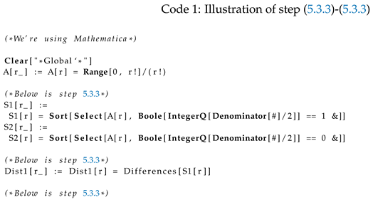
5.3.3. Example of The “Measure” of $\left(G_r^{★}\right)$ Increasing at Rate Super-Linear to that of $\left(G_v^{★★}\right)$

Suppose, we have function $f:A\to \mathbb{R}$, where $A=\mathbb{Q}\cap [0,1]$, and:

$$f\left(x\right)=\left\{\begin{array}{cc}1\hfill & x\in \left\{(2s+1)/\left(2t\right):s\in \mathbb{Z},t\in \mathbb{N},t\ne 0\right\}\cap [0,1]\hfill \\ 0\hfill & x\notin \left\{(2s+1)/\left(2t\right):s\in \mathbb{Z},t\in \mathbb{N},t\ne 0\right\}\cap [0,1]\hfill \end{array}\right.$$

(33)

such that:

$${\left(A_r^{★}\right)}_{r\in \mathbb{N}}={\left(\left\{c/r!:c\in \mathbb{Z},0\le c\le r!\right\}\right)}_{r\in \mathbb{N}}$$

and

$${\left(A_v^{★★}\right)}_{v\in \mathbb{N}}={\left(\left\{c/d:c\in \mathbb{Z},d\in \mathbb{N},d\le v,0\le c\le v\right\}\right)}_{v\in \mathbb{N}}$$

where for $f_r^{★}:A_r^{★}\to \mathbb{R}$,

$$f_r^{★}\left(x\right)=f\left(x\right)\mathrm{for}\mathrm{all}x\in A_r^{★}$$

(34)

and $f_v^{★★}:A_v^{★★}\to \mathbb{R}$

$$f_v^{★★}\left(x\right)=f\left(x\right)\mathrm{for}\mathrm{all}x\in A_v^{★★}$$

(35)

Hence, when ${\left(G_r^{★}\right)}_{r\in \mathbb{N}}$ is:

$${\left(G_r^{★}\right)}_{r\in \mathbb{N}}={\left(\left\{(x,f\left(x\right)):x\in \left\{c/r!:c\in \mathbb{Z},0\le c\le r!\right\}\right\}\right)}_{r\in \mathbb{N}}$$

(36)

and ${\left(G_v^{★★}\right)}_{r\in \mathbb{N}}$ is:

$${\left(G_v^{★★}\right)}_{r\in \mathbb{N}}={\left(\left\{(x,f\left(x\right)):x\in \left\{c/d:c\in \mathbb{Z},d\in \mathbb{N},d\le v,0\le c\le v\right\}\right\}\right)}_{v\in \mathbb{N}}$$

(37)

Note, the following:

Since $\epsilon >0$ and $A=\mathbb{Q}\cap [0,1]$ is countably infinite, there exists minimum $\epsilon$ which is 1. Therefore, we don’t need $\epsilon \to 0$. We also maximize $\mathrm{E}\left(\mathcal{L}\left(\mathcal{S}(\mathbf{C}(\epsilon ,G_r^{★},\omega ),\psi )\right)\right)$ (§5.3.1 step 5.3.10e) by the following procedure:

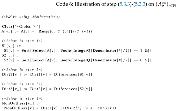
(1)

For every $r\in \mathbb{N}$, group $x\in G_r^{★}$ into elements with an even numerator when simplified: i.e.,

$$x\in \left\{(2s+1)/\left(2t\right):s\in \mathbb{Z},t\in \mathbb{N},t\ne 0\right\}$$

which we call $S_{1,r}$, and group $x\in G_r^{★}$ into elements with an odd denominator when simplified: i.e.,

$$x\in \mathbb{Q}\setminus \left\{(2s+1)/\left(2t\right):s\in \mathbb{Z},t\in \mathbb{N},t\ne 0\right\}$$

which we call $S_{2,r}$

(2)

Arrange the points in $S_{1,r}$ from least to greatest and take the 2-d Euclidean distance between each pair of consecutive points in $S_{1,r}$. In this case, since all points lie on $y=1$, take the absolute difference between the x-coordinates of $S_{1,r}$ then call this ${\mathcal{D}}_{1,r}$. (Note, this is similar to $\S$5.3.1 step 5.3.10a).

(3)

Repeat step (5.3.3) for $S_{2,r}$, then call this ${\mathcal{D}}_{2,r}$. (Note, all point of $S_{2,r}$ lie on $y=0$.)

(4)

Remove any outliers from ${\mathcal{D}}_r={\mathcal{D}}_{1,r}\cup {\mathcal{D}}_{2,r}\cup \left\{d(({\displaystyle \frac{n!-1}{n!}},1),(1,0))\right\}$ (i.e., d is the 2-d Euclidean distance between points $({\displaystyle \frac{n!-1}{n!}},1)$ and $(1,0)$). Note, in this case, ${\mathcal{D}}_{2,r}$ and $\left\{d(({\displaystyle \frac{n!-1}{n!}},1),(1,0))\right\}$ should be outliers (i.e., for any $C>0$, the lengths of ${\mathcal{D}}_{2,r}$ are more than C times the interquartile range of the lengths of ${\mathcal{D}}_r$) leaving us with ${\mathcal{D}}_{1,r}$.

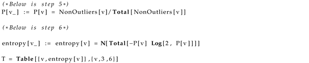
(5)

Multiply the remaining lengths in the pathway by a constant so they add up to one. (See P[r] of code for an example)

(6)

Take the entropy of the probability distribution. (See entropy[r] of code for an example.)

We can illustrate this process with the following code:

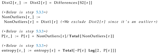
Taking Table[{r,entropy[r]},{r,3,8}], we get

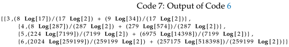
and notice when:

• $c\left(r\right)=(r!)/2-1$
• $\left\{b\left(4\right)\mapsto 9,b\left(5\right)\mapsto 45,b\left(6\right)\mapsto 315,b\left(7\right)\mapsto 2205,b\left(8\right)\mapsto 19845\right\}$
• $a\left(r\right)+b\left(r\right)=c\left(r\right)$

the output of code can be defined:

$${\displaystyle \frac{a\left(r\right){log}_2\left(c\left(r\right)\right)}{c\left(r\right)}}+{\displaystyle \frac{b\left(r\right)log\left(2c\right(r\left)\right))}{c\left(r\right)}}={\displaystyle \frac{a\left(r\right){log}_2\left(c\left(r\right)\right)+b\left(r\right)log\left(2c\left(r\right)\right)}{c\left(r\right)}}$$

(38)

Hence, since $a\left(r\right)=c\left(r\right)-b\left(r\right)=(r!)/2-1-b\left(r\right)$:

$$\begin{array}{cc}\hfill & {\displaystyle \frac{a\left(r\right){log}_2\left(c\left(r\right)\right)+b\left(r\right)log\left(2c\left(r\right)\right)}{c\left(r\right)}}=\hfill \end{array}$$

(39)

$$\begin{array}{cc}\hfill & {\displaystyle \frac{(r!/2-1-b\left(r\right)){log}_2\left(c\left(r\right)\right)+b\left(r\right){log}_2\left(2c\left(r\right)\right)}{c\left(r\right)}}=\hfill \end{array}$$

(40)

$$\begin{array}{cc}\hfill & {\displaystyle \frac{(r!/2){log}_2\left(c\left(r\right)\right)-{log}_2\left(c\left(r\right)\right)-b\left(r\right){log}_2\left(r\right)+b\left(r\right){log}_2\left(c\left(r\right)\right)+b\left(r\right){log}_2\left(2\right)}{c\left(r\right)}}=\hfill \end{array}$$

(41)

$$\begin{array}{cc}\hfill & {\displaystyle \frac{(r!/2){log}_2\left(c\left(r\right)\right)-{log}_2\left(c\left(r\right)\right)+b\left(r\right)}{c\left(r\right)}}=\hfill \end{array}$$

(42)

$$\begin{array}{cc}\hfill & {\displaystyle \frac{(r!/2-1){log}_2\left(c\left(r\right)\right)+b\left(r\right)}{c\left(r\right)}}=\hfill \end{array}$$

(43)

$$\begin{array}{cc}\hfill & {\displaystyle \frac{(r!/2-1){log}_2(r!/2-1)+b\left(r\right)}{r!/2-1}}=\hfill \end{array}$$

(44)

$$\begin{array}{cc}\hfill & {log}_2(r!/2-1)+{\displaystyle \frac{b\left(r\right)}{r!/2-1}}=\hfill \end{array}$$

(45)

and ${lim}_{r\to \infty }b\left(r\right)/c\left(r\right)=1$ (I need help proving this):

$$\begin{array}{cc}\hfill & {log}_2(r!/2-1)+{\displaystyle \frac{b\left(r\right)}{r!/2-1}}\sim {log}_2(r!/2-1)+1\hfill \end{array}$$

(46)

$$\begin{array}{cc}\hfill & {log}_2(r!/2-1)+{log}_2\left(2\right)=\hfill \end{array}$$

(47)

$$\begin{array}{cc}\hfill & {log}_2\left(2(r!/2-1)\right)\hfill \end{array}$$

(48)

$$\begin{array}{cc}\hfill & {log}_2(r!-2)\sim {log}_2(r!)\hfill \end{array}$$

(49)

Hence, entropy[r] is the same as:

$$\begin{array}{cc}\hfill & \mathrm{E}\left(\mathcal{L}\left(\mathcal{S}(\mathbf{C}(1,G_r^{★},\omega ),\psi )\right)\right)\sim {log}_2(r!)\hfill \end{array}$$

(50)

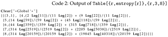
Now, repeat code 1 with:

$${\left(A_v^{★★}\right)}_{r\in \mathbb{N}}=\left(\left\{c/d:c\in \mathbb{Z},d\in \mathbb{N},d\le v,0\le c\le v\right\}\right)$$

Using this post [15], we assume an approximation of Table[entropy[v],{v,3,Infinity}] or

$\mathrm{E}\left(\mathcal{L}\left(\mathcal{S}(\mathbf{C}(1,G_v^{★★},{\omega }^{\prime }),{\psi }^{\prime })\right)\right)$ is:

$$\begin{array}{cc}\hfill & \mathrm{E}\left(\mathcal{L}\left(\mathcal{S}(\mathbf{C}(1,G_v^{★★},{\omega }^{\prime }),{\psi }^{\prime })\right)\right)\sim 2{log}_2\left(v\right)+1-{log}_2\left(3\pi \right)\hfill \end{array}$$

(51)

Hence, using §5.3.2 (0a) and §5.3.2 (5.3.2), take $\left|\mathcal{S}(\mathbf{C}(\epsilon ,G_v^{★★},{\omega }^{\prime }),{\psi }^{\prime })\right|={\sum }_{M=1}^v\varphi \left(M\right)\approx {\displaystyle \frac{3}{{\pi }^2}}{v}^2$ (where $\varphi$ is Euler’s Totient function) computing the following:

$$\begin{array}{cc}& \underline{\left|\mathcal{S}(\mathbf{C}(\epsilon ,G_r^{★},\omega ),\psi )\right|}=\hfill \\ \hfill & sup\left\{\left|\mathcal{S}(\mathbf{C}(\epsilon ,G_v^{★★},{\omega }^{\prime }),{\psi }^{\prime })\right|:v\in \mathbb{N},{\omega }^{\prime }\in {\Omega }_{\epsilon ,v},{\psi }^{\prime }\in {\Psi }_{\epsilon ,v,\omega },\mathrm{E}\left(\mathcal{L}\left(\mathcal{S}(\mathbf{C}(\epsilon ,G_v^{★★},{\omega }^{\prime }),{\psi }^{\prime })\right)\right)\le \mathrm{E}\left(\mathcal{L}\left(\mathcal{S}(\mathbf{C}(\epsilon ,G_r^{★},\omega ),\psi )\right)\right)\right\}=\hfill \\ \hfill & sup\left\{{\displaystyle \frac{3}{{\pi }^2}}{v}^2:v\in \mathbb{N},{\omega }^{\prime }\in {\Omega }_{\epsilon ,v},{\psi }^{\prime }\in {\Psi }_{\epsilon ,v,\omega },2{log}_2\left(v\right)+1-{log}_2\left(3\pi \right)\le {log}_2(r!)\right\}=\hfill \end{array}$$

(52)

where:

(1)

For every $r\in \mathbb{N}$, we find a $v\in \mathbb{N}$, where $2{log}_2\left(r\right)+1-{log}_2\left(3\pi \right)\le {log}_2(r!)$, but the absolute value of ${log}_2(r!)-\left(2{log}_2\left(v\right)+1-{log}_2\left(3\pi \right)\right)$ is minimized. In other words, for every $r\in \mathbb{N}$, we want $v\in \mathbb{N}$ where:

$$\begin{array}{cc}\hfill & 2{log}_2\left(v\right)+1-{log}_2\left(3\pi \right)\le {log}_2(r!)\hfill \end{array}$$

(53)

$$\begin{array}{cc}\hfill & 2{log}_2\left(v\right)\le {log}_2(r!)-1+{log}_2\left(3\pi \right)\hfill \end{array}$$

(54)

$$\begin{array}{cc}\hfill & {\left(2^{{log}_2\left(v\right)}\right)}^2\le 2^{{log}_2(r!)-1+{log}_2\left(3\pi \right)}\hfill \end{array}$$

(55)

$$\begin{array}{cc}\hfill & {\left(v\right)}^2\le \left(2^{{log}_2(r!)}{2}^{{log}_2\left(3\pi \right)}\right)/2\hfill \end{array}$$

(56)

$$\begin{array}{cc}\hfill & v\le \sqrt{{\displaystyle \frac{r!\left(3\pi \right)}{2}}}\hfill \end{array}$$

(57)

$$\begin{array}{cc}\hfill & v=⌊\sqrt{{\displaystyle \frac{3\pi r!}{2}}}⌋\hfill \end{array}$$

(58)

$$\begin{array}{cc}\hfill & {\displaystyle \frac{3}{{\pi }^2}}{v}^2={\displaystyle \frac{3}{{\pi }^2}}{\left(⌊\sqrt{{\displaystyle \frac{3\pi r!}{2}}}⌋\right)}^2\sim \underline{\left|\mathcal{S}(\mathbf{C}(1,G_r^{★},\omega ),\psi )\right|}\hfill \end{array}$$

(59)

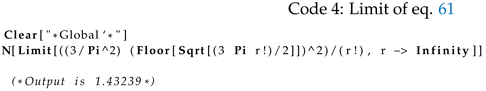
Finally, since $\left|\mathcal{S}(\mathbf{C}(\epsilon ,G_r^{★},\omega ),\psi )\right|=r!$, we wish to prove

$$1<\underset{\epsilon \to 0}{lim\; inf}\underset{r\to \infty }{lim\; inf}\underset{\omega \in {\Omega }_{\epsilon ,r}}{inf}\underset{\psi \in {\Psi }_{\epsilon ,r,\omega }}{inf}\underline{\alpha }\left(\epsilon ,r,\omega ,\psi \right)<+\infty$$

within §5.3.2 crit. 5.3.2:

$$\begin{array}{cc}\hfill & \underset{\epsilon \to 0}{lim\; inf}\underset{r\to \infty }{lim\; inf}\underset{\omega \in {\Omega }_{\epsilon ,r}}{inf}\underset{\psi \in {\Psi }_{\epsilon ,r,\omega }}{inf}\underline{\alpha }\left(\epsilon ,r,\omega ,\psi \right)=\underset{r\to \infty }{lim\; inf}\underset{\omega \in {\Omega }_{\epsilon ,r}}{inf}\underset{\psi \in {\Psi }_{\epsilon ,r,\omega }}{inf}{\displaystyle \frac{\underline{\left|\mathcal{S}(\mathbf{C}(1,G_r^{★},\omega ),\psi )\right|}}{\left|\mathcal{S}(\mathbf{C}(1,G_r^{★},\omega ),\psi ))\right|}}\hfill \end{array}$$

(60)

$$\begin{array}{cc}\hfill & =\underset{r\to \infty }{lim}{\displaystyle \frac{\frac{3}{{\pi }^2}{\left(⌊\sqrt{\frac{3\pi r!}{2}}⌋\right)}^2}{r!}}\hfill \end{array}$$

(61)

where using mathematica, we get the limit is greater than one:

Also, using §5.3.2 (1b) and §5.3.2 (2), take $\left|\mathcal{S}(\mathbf{C}(\epsilon ,G_v^{★★},{\omega }^{\prime }),{\psi }^{\prime })\right|={\sum }_{M=1}^r\varphi \left(M\right)\approx {\displaystyle \frac{3}{{\pi }^2}}{r}^2$ (where $\varphi$ is Euler’s Totient function) to compute the following:

$$\begin{array}{cc}& \underline{\left|\mathcal{S}(\mathbf{C}(\epsilon ,G_r^{★},\omega ),\psi )\right|}=\hfill \\ \hfill & inf\left\{\left|\mathcal{S}(\mathbf{C}(\epsilon ,G_v^{★★},{\omega }^{\prime }),{\psi }^{\prime })\right|:v\in \mathbb{N},{\omega }^{\prime }\in {\Omega }_{\epsilon ,v},{\psi }^{\prime }\in {\Psi }_{\epsilon ,v,\omega },\mathrm{E}\left(\mathcal{L}\left(\mathcal{S}(\mathbf{C}(\epsilon ,G_v^{★★},{\omega }^{\prime }),{\psi }^{\prime })\right)\right)\ge \mathrm{E}\left(\mathcal{L}\left(\mathcal{S}(\mathbf{C}(\epsilon ,G_r^{★},\omega ),\psi )\right)\right)\right\}=\hfill \\ \hfill & inf\left\{{\displaystyle \frac{3}{{\pi }^2}}{v}^2:r\in \mathbb{N},{\omega }^{\prime }\in {\Omega }_{\epsilon ,v},{\psi }^{\prime }\in {\Psi }_{\epsilon ,v,\omega },2{log}_2\left(v\right)+1-{log}_2\left(3\pi \right)\ge {log}_2(r!)\right\}=\hfill \end{array}$$

(62)

where:

(1)

For every $r\in \mathbb{N}$, we find a $v\in \mathbb{N}$, where $2{log}_2\left(v\right)+1-{log}_2\left(3\pi \right)\ge {log}_2(r!)$, but the absolute value of $\left(2{log}_2\left(v\right)+1-{log}_2\left(3\pi \right)\right)-{log}_2(r!)$ is minimized. In other words,

for every $r\in \mathbb{N}$, we want $v\in \mathbb{N}$ where:

$$\begin{array}{cc}\hfill & 2{log}_2\left(v\right)+1-{log}_2\left(3\pi \right)\ge {log}_2(r!)\hfill \end{array}$$

(63)

$$\begin{array}{cc}\hfill & 2^{2{log}_2\left(v\right)}\ge {log}_2(r!)-1+{log}_2\left(3\pi \right)\hfill \end{array}$$

(64)

$$\begin{array}{cc}\hfill & {\left(2^{{log}_2\left(v\right)}\right)}^2\ge 2^{{log}_2(r!)-1+{log}_2\left(3\pi \right)}\hfill \end{array}$$

(65)

$$\begin{array}{cc}\hfill & v^2\ge \left(2^{{log}_2(r!)}{2}^{{log}_2\left(3\pi \right)}\right)/2\hfill \end{array}$$

(66)

$$\begin{array}{cc}\hfill & v\ge \sqrt{{\displaystyle \frac{r!\left(3\pi \right)}{2}}}\hfill \end{array}$$

(67)

$$\begin{array}{cc}\hfill & v=⌈\sqrt{{\displaystyle \frac{3\pi r!}{2}}}⌉\hfill \end{array}$$

(68)

$$\begin{array}{cc}\hfill & {\displaystyle \frac{3}{{\pi }^2}}{v}^2={\displaystyle \frac{3}{{\pi }^2}}{\left(⌈\sqrt{{\displaystyle \frac{3\pi r!}{2}}}⌉\right)}^2\sim \overline{\left|\mathcal{S}(\mathbf{C}(1,G_r^{★},\omega ),\psi )\right|}\hfill \end{array}$$

(69)

Finally, since $\left|\mathcal{S}(\mathbf{C}(1,G_r^{★},\omega ),\psi )\right|=r!$, we wish to prove

$$1<\underset{\epsilon \to 0}{lim\; sup}\underset{r\to \infty }{lim\; sup}\underset{\omega \in {\Omega }_{\epsilon ,r}}{sup}\underset{\psi \in {\Psi }_{\epsilon ,r,\omega }}{sup}\overline{\alpha }\left(\epsilon ,r,\omega ,\psi \right)<+\infty$$

within §5.3.2 crit. 5.3.2:

$$\begin{array}{cc}\hfill & \underset{\epsilon \to 0}{lim\; sup}\underset{r\to \infty }{lim\; sup}\underset{\omega \in {\Omega }_{\epsilon ,r}}{sup}\underset{\psi \in {\Psi }_{\epsilon ,r,\omega }}{sup}\overline{\alpha }\left(\epsilon ,r,\omega ,\psi \right)=\underset{r\to \infty }{lim\; sup}\underset{\omega \in {\Omega }_{\epsilon ,r}}{sup}\underset{\psi \in {\Psi }_{\epsilon ,r,\omega }}{sup}{\displaystyle \frac{\overline{\left|\mathcal{S}(\mathbf{C}(1,G_r^{★},\omega ),\psi )\right|}}{\left|\mathcal{S}(\mathbf{C}(1,G_r^{★},\omega ),\psi ))\right|}}\hfill \end{array}$$

(70)

$$\begin{array}{cc}\hfill & =\underset{r\to \infty }{lim}{\displaystyle \frac{\frac{3}{{\pi }^2}{\left(⌈\sqrt{\frac{3\pi r!}{2}}⌉\right)}^2}{r!}}\hfill \end{array}$$

(71)

where using mathematica, we get the limit is greater than one:

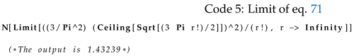
Hence, since the limits in eq. 61 and eq. 71 are greater than one and less than $+\infty$: i.e.,

$$1<\underset{\epsilon \to 0}{lim\; inf}\underset{r\to \infty }{lim\; inf}\underset{\omega \in {\Omega }_{\epsilon ,r}}{inf}\underset{\psi \in {\Psi }_{\epsilon ,r,\omega }}{inf}\underline{\alpha }\left(\epsilon ,r,\omega ,\psi \right)=\underset{\epsilon \to 0}{lim\; sup}\underset{r\to \infty }{lim\; sup}\underset{\omega \in {\Omega }_{\epsilon ,r}}{sup}\underset{\psi \in {\Psi }_{\epsilon ,r,\omega }}{sup}\overline{\alpha }\left(\epsilon ,r,\omega ,\psi \right)<+\infty$$

(72)

what we’re measuring from${\left(G_r^{★}\right)}_{r\in \mathbb{N}}$ increases at a rate superlinear to that of ${\left(G_v^{★★}\right)}_{r\in \mathbb{N}}$ (i.e., 5.3.2 crit. 5.3.2).

5.3.4. Example of The “Measure" from ${\left(G_r^{★}\right)}_{r\in \mathbb{N}}$ Increasing at a Rate Sub-Linear to that of ${\left(G_v^{★★}\right)}_{j\in \mathbb{N}}$

Using our previous example, we can use the following theorem:

Theorem 8. 

If what we’re measuring from ${\left(G_r^{★}\right)}_{r\in \mathbb{N}}$ increases at a rate superlinear to that of ${\left(G_v^{★★}\right)}_{r\in \mathbb{N}}$, then what we’re measuring from ${\left(G_v^{★★}\right)}_{r\in \mathbb{N}}$ increases at a ratesublinearto that of ${\left(G_r^{★}\right)}_{r\in \mathbb{N}}$

Hence, in our definition of super-linear (§5.3.2 crit. 5.3.2), swap $G_r^{★}$ for $G_v^{★★}$and$j\in \mathbb{N}$ for $r\in \mathbb{N}$ regarding $\overline{\alpha }\left(ϵ,r,\omega ,\psi \right)$ and $\underline{\alpha }\left(ϵ,r,\omega ,\psi \right)$ (i.e., $\overline{\alpha }\left(ϵ,v,\omega ,\psi \right)$ and $\underline{\alpha }\left(ϵ,v,\omega ,\psi \right)$) and notice thm. 8 is true when:

$$1<\underset{\epsilon \to 0}{lim\; sup}\underset{v\to \infty }{lim\; sup}\underset{\omega \in {\Omega }_{\epsilon ,v}}{sup}\underset{\psi \in {\Psi }_{\epsilon ,v,\omega }}{sup}\overline{\alpha }\left(\epsilon ,v,\omega ,\psi \right),\underset{\epsilon \to 0}{lim\; inf}\underset{v\to \infty }{lim\; inf}\underset{\omega \in {\Omega }_{\epsilon ,v}}{inf}\underset{\psi \in {\Psi }_{\epsilon ,v,\omega }}{inf}\underline{\alpha }\left(\epsilon ,v,\omega ,\psi \right)<+\infty$$

5.3.5. Example of The “Measure" from ${\left(G_r^{★}\right)}_{r\in \mathbb{N}}$ Increasing at a Rate Linear to that of ${\left(G_v^{★★}\right)}_{r\in \mathbb{N}}$

Suppose, we have function $f:A\to \mathbb{R}$, where $A=\mathbb{Q}\cap [0,1]$, and:

$$f\left(x\right)=\left\{\begin{array}{cc}1\hfill & x\in \left\{(2s+1)/\left(2t\right):s\in \mathbb{Z},t\in \mathbb{N},t\ne 0\right\}\cap [0,1]\hfill \\ 0\hfill & x\notin \left\{(2s+1)/\left(2t\right):s\in \mathbb{Z},t\in \mathbb{N},t\ne 0\right\}\cap [0,1]\hfill \end{array}\right.$$

(73)

such that:

$${\left(A_r^{★}\right)}_{r\in \mathbb{N}}={\left(\left\{c/r!:c\in \mathbb{Z},0\le c\le r!\right\}\right)}_{r\in \mathbb{N}}$$

and

$${\left(A_v^{★★}\right)}_{v\in \mathbb{N}}=\left(\left\{c/{(v!)}^2:c\in \mathbb{N},1\le c\le {(v!)}^2\right\}\right)$$

where for $f_r^{★}:A_r^{★}\to \mathbb{R}$,

$$f_r^{★}\left(x\right)=f\left(x\right)\mathrm{for}\mathrm{all}x\in A_r^{★}$$

(74)

and $f_v^{★★}:A_v^{★★}\to \mathbb{R}$

$$f_v^{★★}\left(x\right)=f\left(x\right)\mathrm{for}\mathrm{all}x\in A_v^{★★}$$

(75)

Hence, when ${\left(G_r^{★}\right)}_{r\in \mathbb{N}}$ is:

$${\left(G_r^{★}\right)}_{r\in \mathbb{N}}={\left(\left\{(x,f\left(x\right)):x\in \left\{c/r!:c\in \mathbb{Z},0\le c\le r!\right\}\right\}\right)}_{r\in \mathbb{N}}$$

(76)

and ${\left(G_v^{★★}\right)}_{r\in \mathbb{N}}$ is:

$${\left(G_v^{★★}\right)}_{r\in \mathbb{N}}={\left(\left\{(x,f\left(x\right)):x\in \left\{c/{(v!)}^2:c\in \mathbb{Z},0\le c\le {(v!)}^2\right\}\right\}\right)}_{r\in \mathbb{N}}$$

(77)

We already know, using eq. 50:

$$\mathrm{E}\left(\mathcal{L}\left(\mathcal{S}(\mathbf{C}(1,G_r^{★},\omega ),\psi )\right)\right)\sim {log}_2(r!-2)\sim {log}_2(r!)$$

(78)

Also, using § 5.3.3 steps 5.3.3-5.3.3 on ${\left(A_v^{★★}\right)}_{r\in \mathbb{N}}$:

where the output is

Notice when:

(1)

$c\left(v\right)={(v!)}^2/2-1$

(2)

$\left\{b\left(4\right)\mapsto 9,b\left(5\right)\mapsto 279,b\left(6\right)\mapsto 6975,b\left(7\right)\mapsto 257175,b\left(8\right)\mapsto 19845\right\}$

(3)

$a\left(v\right)+b\left(v\right)=c\left(v\right)$

the output of code can be defined:

$${\displaystyle \frac{a\left(v\right){log}_2\left(c\left(v\right)\right)}{c\left(v\right)}}+{\displaystyle \frac{b\left(v\right)log\left(2c\right(v\left)\right)}{c\left(v\right)}}={\displaystyle \frac{a\left(v\right){log}_2\left(c\left(v\right)\right)+b\left(v\right)log\left(2c\left(v\right)\right)}{c\left(v\right)}}$$

(79)

Hence, since $a\left(v\right)=c\left(v\right)-b\left(v\right)={(v!)}^2/2-1-b\left(v\right)$:

$$\begin{array}{cc}\hfill & {\displaystyle \frac{a\left(v\right){log}_2\left(c\left(v\right)\right)+b\left(v\right)log\left(2c\left(v\right)\right)}{c\left(v\right)}}=\hfill \end{array}$$

(80)

$$\begin{array}{cc}\hfill & {\displaystyle \frac{({(v!)}^2/2-1-b\left(v\right)){log}_2\left(c\left(v\right)\right)+b\left(v\right){log}_2\left(2c\left(v\right)\right)}{c\left(v\right)}}=\hfill \end{array}$$

(81)

$$\begin{array}{cc}\hfill & {\displaystyle \frac{({(v!)}^2/2){log}_2\left(c\left(v\right)\right)-{log}_2\left(c\left(v\right)\right)-b\left(v\right){log}_2\left(v\right)+b\left(v\right){log}_2\left(c\left(v\right)\right)+b\left(v\right){log}_2\left(2\right)}{c\left(v\right)}}=\hfill \end{array}$$

(82)

$$\begin{array}{cc}\hfill & {\displaystyle \frac{({(v!)}^2/2){log}_2\left(c\left(v\right)\right)-{log}_2\left(c\left(v\right)\right)+b\left(v\right)}{c\left(v\right)}}=\hfill \end{array}$$

(83)

$$\begin{array}{cc}\hfill & {\displaystyle \frac{({(v!)}^2/2-1){log}_2\left(c\left(v\right)\right)+b\left(v\right)}{c\left(v\right)}}=\hfill \end{array}$$

(84)

$$\begin{array}{cc}\hfill & {\displaystyle \frac{({(v!)}^2/2-1){log}_2({(v!)}^2/2-1)+b\left(v\right)}{{(v!)}^2/2-1}}=\hfill \end{array}$$

(85)

$$\begin{array}{cc}\hfill & {log}_2({(v!)}^2/2-1)+{\displaystyle \frac{b\left(v\right)}{{(v!)}^2/2-1}}=\hfill \end{array}$$

(86)

since ${lim}_{v\to \infty }b\left(v\right)/c\left(v\right)=1$ (this is proven in [16]):

$$\begin{array}{cc}\hfill & {log}_2({(v!)}^2/2-1)+{\displaystyle \frac{b\left(v\right)}{{(v!)}^2/2-1}}\sim {log}_2({(v!)}^2/2-1)+1\hfill \end{array}$$

(87)

$$\begin{array}{cc}\hfill & {log}_2({(v!)}^2/2-1)+{log}_2\left(2\right)=\hfill \end{array}$$

(88)

$$\begin{array}{cc}\hfill & {log}_2({(v!)}^2-2))\sim \hfill \end{array}$$

(89)

$$\begin{array}{cc}\hfill & {log}_2\left({(v!)}^2\right)=\hfill \end{array}$$

(90)

$$\begin{array}{cc}\hfill & 2{log}_2(v!)\hfill \end{array}$$

(91)

Hence, entropy[r] is the same as:

$$\begin{array}{cc}\hfill & \mathrm{E}\left(\mathcal{L}\left(\mathcal{S}(\mathbf{C}(1,G_v^{★★},\omega ),\psi )\right)\right)\sim \hfill \end{array}$$

(92)

$$\begin{array}{cc}\hfill & 2{log}_2(v!)\hfill \end{array}$$

(93)

Therefore, using §5.3.2 (0a) and §5.3.2 (5.3.20a), take $\left|\mathcal{S}(\mathbf{C}(\epsilon ,G_v^{★★},{\omega }^{\prime }),{\psi }^{\prime })\right|={(v!)}^2$ to compute the following:

$$\begin{array}{cc}& \underline{\left|\mathcal{S}(\mathbf{C}(\epsilon ,G_r^{★},\omega ),\psi )\right|}=\hfill \\ \hfill & sup\left\{\left|\mathcal{S}(\mathbf{C}(\epsilon ,G_v^{★★},{\omega }^{\prime }),{\psi }^{\prime })\right|:v\in \mathbb{N},{\omega }^{\prime }\in {\Omega }_{\epsilon ,v},{\psi }^{\prime }\in {\Psi }_{\epsilon ,v,\omega },\mathrm{E}\left(\mathcal{L}\left(\mathcal{S}(\mathbf{C}(\epsilon ,G_v^{★★},{\omega }^{\prime }),{\psi }^{\prime })\right)\right)\le \mathrm{E}\left(\mathcal{L}\left(\mathcal{S}(\mathbf{C}(\epsilon ,G_r^{★},\omega ),\psi )\right)\right)\right\}=\hfill \\ \hfill & sup\left\{{(v!)}^2:r\in \mathbb{N},{\omega }^{\prime }\in {\Omega }_{\epsilon ,v},{\psi }^{\prime }\in {\Psi }_{\epsilon ,v,\omega },2{log}_2(v!)\le {log}_2(r!)\right\}=\hfill \end{array}$$

(94)

where:

(1)

For every $r\in \mathbb{N}$, we find a $v\in \mathbb{N}$, where $2{log}_2(v!)\le {log}_2(r!)$, but the absolute value of ${log}_2(r!)-2{log}_2(v!)$ is minimized. In other words, for every $r\in \mathbb{N}$, we want $v\in \mathbb{N}$ where:

$$\begin{array}{cc}\hfill & 2{log}_2(v!)\le {log}_2(r!)\hfill \end{array}$$

(95)

$$\begin{array}{cc}\hfill & 2^{2{log}_2(v!)}\le 2^{{log}_2(r!)}\hfill \end{array}$$

(96)

$$\begin{array}{cc}\hfill & {\left(2^{{log}_2(v!)}\right)}^2\le r!\hfill \end{array}$$

(97)

$$\begin{array}{cc}\hfill & {(v!)}^2\le r!\hfill \end{array}$$

(98)

$$\begin{array}{cc}\hfill & {(v!)}^2=\lfloor r!\rfloor \hfill \end{array}$$

(99)

To solve for v, we try the following code:

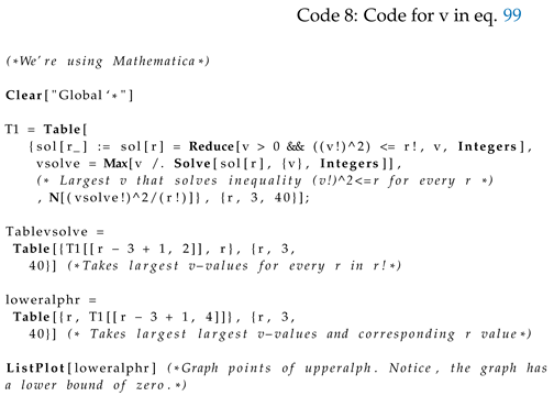
Note, the output is:

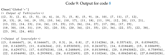
Figure 1. Plot of loweralphr.

Figure 1. Plot of loweralphr.

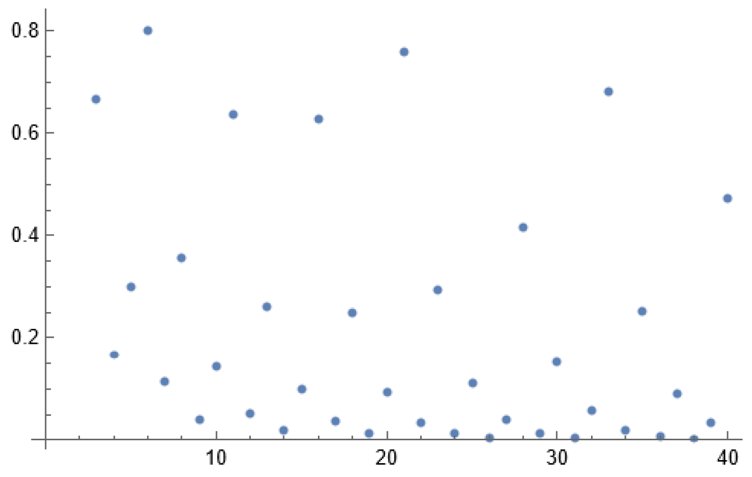
Finally, since the lower bound of loweralphr is zero, we have shown:

$$\underset{\epsilon \to 0}{lim\; inf}\underset{r\to \infty }{lim\; inf}\underset{\omega \in {\Omega }_{\epsilon ,r}}{inf}\underset{\psi \in {\Psi }_{\epsilon ,r,\omega }}{inf}\underline{\alpha }\left(\epsilon ,r,\omega ,\psi \right)=0$$

(100)

Next, using §5.3.2 (0b) and §5.3.2 (5.3.2), take $\left|\mathcal{S}(\mathbf{C}(\epsilon ,G_r^{★},{\omega }^{\prime }),{\psi }^{\prime })\right|=r!$ and swap $r\in \mathbb{N}$ and ${\left(G_r^{★}\right)}_{r\in \mathbb{N}}$ with $r\in \mathbb{N}$ and ${\left(G_v^{★★}\right)}_{r\in \mathbb{N}}$, to compute the following:

$$\begin{array}{cc}& \underline{\left|\mathcal{S}(\mathbf{C}(\epsilon ,G_v^{★★},\omega ),\psi )\right|}=\hfill \\ \hfill & inf\left\{\left|\mathcal{S}(\mathbf{C}(\epsilon ,G_r^{★},{\omega }^{\prime }),{\psi }^{\prime })\right|:r\in \mathbb{N},{\omega }^{\prime }\in {\Omega }_{\epsilon ,r},{\psi }^{\prime }\in {\Psi }_{\epsilon ,r,\omega },\mathrm{E}\left(\mathcal{L}\left(\mathcal{S}(\mathbf{C}(\epsilon ,G_r^{★},{\omega }^{\prime }),{\psi }^{\prime })\right)\right)\ge \mathrm{E}\left(\mathcal{L}\left(\mathcal{S}(\mathbf{C}(\epsilon ,G_v^{★★},\omega ),\psi )\right)\right)\right\}=\hfill \\ \hfill & inf\left\{r!:r\in \mathbb{N},{\omega }^{\prime }\in {\Omega }_{\epsilon ,r},{\psi }^{\prime }\in {\Psi }_{\epsilon ,r,\omega },{log}_2(r!)\ge 2{log}_2(v!)\right\}=\hfill \end{array}$$

(101)

where:

(1)

For every $v\in \mathbb{N}$, we find a $r\in \mathbb{N}$, where ${log}_2(r!)\le 2{log}_2(v!)$, but the absolute value of $2{log}_2(v!)-{log}_2(r!)$ is minimized. In other words, for every $v\in \mathbb{N}$, we want $r\in \mathbb{N}$ where:

$$\begin{array}{cc}\hfill & {log}_2(r!)\le 2{log}_2(v!)\hfill \end{array}$$

(102)

$$\begin{array}{cc}\hfill & 2^{{log}_2(r!)}\le 2^{2{log}_2(v!)}\hfill \end{array}$$

(103)

$$\begin{array}{cc}\hfill & r!\le {\left(2^{{log}_2(v!)}\right)}^2\hfill \end{array}$$

(104)

$$\begin{array}{cc}\hfill & r!\le {(v!)}^2\hfill \end{array}$$

(105)

$$\begin{array}{cc}\hfill & r!={(v!)}^2\hfill \end{array}$$

(106)

To solve r, we try the following code:

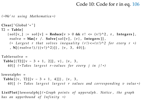
Note, the output is:

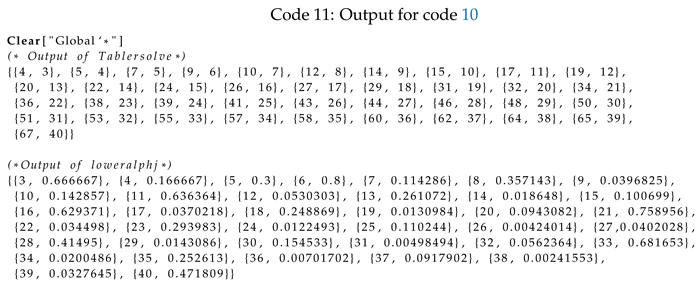
Figure 2. Plot of loweralphj.

Figure 2. Plot of loweralphj.

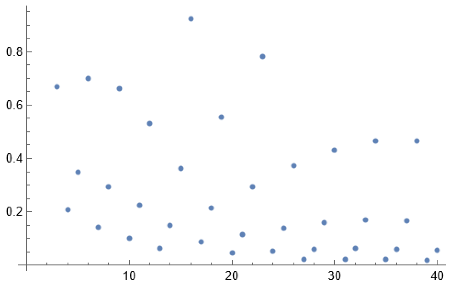
since the lower bound of loweralphj is zero, we have shown:

$$\underset{\epsilon \to 0}{lim\; inf}\underset{v\to \infty }{lim\; inf}\underset{\omega \in {\Omega }_{\epsilon ,v}}{inf}\underset{\psi \in {\Psi }_{\epsilon ,v,\omega }}{inf}\underline{\alpha }\left(\epsilon ,v,\omega ,\psi \right)=0$$

(107)

Hence, using eq. 100 and 107, since both:  

(1)

$\underset{\epsilon \to 0}{lim\; sup}\underset{r\to \infty }{lim\; sup}\underset{\omega \in {\Omega }_{\epsilon ,r}}{sup}\underset{\psi \in {\Psi }_{\epsilon ,r,\omega }}{sup}\overline{\alpha }\left(\epsilon ,r,\omega ,\psi \right)$ or $\underset{\epsilon \to 0}{lim\; inf}\underset{r\to \infty }{lim\; inf}\underset{\omega \in {\Omega }_{\epsilon ,r}}{inf}\underset{\psi \in {\Psi }_{\epsilon ,r,\omega }}{inf}\underline{\alpha }\left(\epsilon ,r,\omega ,\psi \right)$ are equal to zero, one or $+\infty$

(2)

$\underset{\epsilon \to 0}{lim\; sup}\underset{v\to \infty }{lim\; sup}\underset{\omega \in {\Omega }_{\epsilon ,v}}{sup}\underset{\psi \in {\Psi }_{\epsilon ,v,\omega }}{sup}\overline{\alpha }\left(\epsilon ,v,\omega ,\psi \right)$ or $\underset{\epsilon \to 0}{lim\; inf}\underset{v\to \infty }{lim\; inf}\underset{\omega \in {\Omega }_{\epsilon ,v}}{inf}\underset{\psi \in {\Psi }_{\epsilon ,v,\omega }}{inf}\underline{\alpha }\left(\epsilon ,v,\omega ,\psi \right)$ are equal to zero, one or $+\infty$

then what I’m measuring from ${\left(G_r^{★}\right)}_{r\in \mathbb{N}}$ increases at a rate linear to that of ${\left(G_v^{★★}\right)}_{r\in \mathbb{N}}$.

5.4. Defining The Actual Rate of Expansion of Sequence of Bounded Sets

5.4.1. Definition of Actual Rate of Expansion of Sequence of Bounded Sets

Suppose, ${\left(G_r^{★}\right)}_{r\in \mathbb{N}}$ is the sequence of the graph for each function $f_r^{★}$ (§2.3.1). When $d(Q,R)$ is the Euclidean distance between points $Q,R\in {\mathbb{R}}^n$ and a “chosen" center point is $C\in {\mathbb{R}}^{n+1}$, where

$$\mathcal{G}(C,G_r^{★})=sup\left\{d(C,y):y\in G_r^{★}\right\}$$

the actual rate of expansion is:

$$\mathcal{E}(C,G_r^{★})=\mathcal{G}(C,G_{r+1}^{★})-\mathcal{G}(C,G_r^{★})$$

Note, there are cases of ${\left(G_r^{★}\right)}_{r\in \mathbb{N}}$ when $\mathcal{E}$ isn’t fixed and $\mathcal{E}\ne E$ (i.e., the expected, fixed rate of expansion).

5.4.2. Example

Suppose, we have $f:A\to \mathbb{R}$, where $A=\mathbb{R}$ and $f\left(x\right)=x$, such that ${\left(A_r^{★}\right)}_{r\in \mathbb{N}}={\left([-r,r]\right)}_{r\in \mathbb{N}}$ and for $f_r^{★}:A_r^{★}\to \mathbb{R}$:

$$f_r^{★}\left(x\right)=f\left(x\right)\mathrm{for}\mathrm{all}x\in A_r^{★}$$

Hence, when ${\left(G_r^{★}\right)}_{r\in \mathbb{N}}$ is:

$${\left(G_r^{★}\right)}_{r\in \mathbb{N}}={\left(\left\{(x,x):x\in [-r,r]\right\}\right)}_{r\in \mathbb{N}}$$

such that $C=(0,0)$, note the farthest point of $G_r^{★}$ from C is either $(-r,-r)$ or $(r,r)$. Hence, to compute $\mathcal{G}(C,G_r^{★})$, we can take $d\left(\right(0,0),(r,r\left)\right)$ or $d\left(\right(0,0),(-r,r\left)\right)$:

$$\begin{array}{cc}\hfill \mathcal{G}(C,G_r^{★})=& sup\{d(C,y):y\in G_r^{★}\}=\hfill \end{array}$$

(108)

$$\begin{array}{cc}\hfill & d\left(\right(0,0),(r,r\left)\right)=\hfill \end{array}$$

(109)

$$\begin{array}{cc}\hfill & \sqrt{{(0-r)}^2+{(0-r)}^2}=\hfill \end{array}$$

(110)

$$\begin{array}{cc}\hfill & \sqrt{r^2+r^2}=\hfill \end{array}$$

(111)

$$\begin{array}{cc}\hfill & \sqrt{2r^2}=\hfill \end{array}$$

(112)

$$\begin{array}{cc}\hfill & \sqrt{2r^2}=\hfill \end{array}$$

(113)

$$\begin{array}{cc}\hfill & \sqrt{2}\left|r\right|\hfill \end{array}$$

(114)

$$\begin{array}{cc}\hfill & \sqrt{2}r\sin \mathrm{ce}r>0\hfill \end{array}$$

(115)

and the actual rate of expansion is:

$$\begin{array}{cc}\hfill \mathcal{E}(C,G_r^{★})=& \mathcal{G}(C,G_{r+1}^{★})-\mathcal{G}(C,G_r^{★})=\hfill \end{array}$$

(116)

$$\begin{array}{cc}\hfill & \sqrt{2}(r+1)-\sqrt{2}r=\hfill \end{array}$$

(117)

$$\begin{array}{cc}\hfill & \sqrt{2}(r+1)-\sqrt{2}r=\hfill \end{array}$$

(118)

$$\begin{array}{cc}\hfill & \sqrt{2}r+\sqrt{2}-\sqrt{2}r=\hfill \end{array}$$

(119)

$$\begin{array}{cc}\hfill & \sqrt{2}\hfill \end{array}$$

(120)

5.5. Reminder

See if §3.1 is easier to understand.

6. My Attempt At Answering The Approach of §2.5.1

6.1. Choice Function

Suppose we define the following:

(1)

If $\mathcal{B}\subset \mathbf{B}\left({\mathbb{R}}^A\right)$ (§2.3.3) and $\mathcal{B}\subset \mathbf{B}\left(2^{{\mathbb{R}}^n}\right)$ (§2.3.3) are arbitrary sets, then $f_r^{★}\in \mathcal{B}$ and $A_r^{★}\in \mathcal{B}$ satisfy (3.1), (3.1), (3.1), (3.1) and (3.1) of the leading question in $\S$3.1

(2)

$f_v^{★★}\in \mathbf{B}\left({\mathbb{R}}^A\right)\setminus \mathcal{B}$ and $A_v^{★★}\in \mathbf{B}\left(2^{{\mathbb{R}}^n}\right)\setminus \mathcal{B}$

Further note, from §5.3.2 (0b), if we take:

$$\begin{array}{cc}& \overline{\left|\mathcal{S}(\mathbf{C}(\epsilon ,G_r^{★},\omega ),\psi )\right|}=\hfill \\ & inf\left\{\left|\mathcal{S}(\mathbf{C}(\epsilon ,G_v^{★★},{\omega }^{\prime }),{\psi }^{\prime })\right|:v\in \mathbb{N},{\omega }^{\prime }\in {\Omega }_{\epsilon ,v},{\psi }^{\prime }\in {\Psi }_{\epsilon ,v,\omega },\mathrm{E}\left(\mathcal{L}\left(\mathcal{S}(\mathbf{C}(\epsilon ,G_v^{★★},{\omega }^{\prime }),{\psi }^{\prime })\right)\right)\ge \mathrm{E}\left(\mathcal{L}\left(\mathcal{S}(\mathbf{C}(\epsilon ,G_r^{★},\omega ),\psi )\right)\right)\right\}\hfill \end{array}$$

(121)

and from §5.3.2 (0a), we take:

$$\begin{array}{cc}& \underline{\left|\mathcal{S}(\mathbf{C}(\epsilon ,G_r^{★},\omega ),\psi )\right|}=\hfill \\ \hfill & sup\left\{\left|\mathcal{S}(\mathbf{C}(\epsilon ,G_v^{★★},{\omega }^{\prime }),{\psi }^{\prime })\right|:v\in \mathbb{N},{\omega }^{\prime }\in {\Omega }_{\epsilon ,v},{\psi }^{\prime }\in {\Psi }_{\epsilon ,v,\omega },\mathrm{E}\left(\mathcal{L}\left(\mathcal{S}(\mathbf{C}(\epsilon ,G_v^{★★},{\omega }^{\prime }),{\psi }^{\prime })\right)\right)\le \mathrm{E}\left(\mathcal{L}\left(\mathcal{S}(\mathbf{C}(\epsilon ,G_r^{★},\omega ),\psi )\right)\right)\right\}\hfill \end{array}$$

(122)

Then, §5.3.1 (5.3.1), eq. 121, and eq. 122 is:

$$\begin{array}{c}\underset{\omega \in {\Omega }_{\epsilon ,r}}{sup}\underset{\psi \in {\Psi }_{\epsilon ,r,\omega }}{sup}\left|\mathcal{S}(\mathbf{C}(\epsilon ,G_r^{★},\omega ),\psi )\right|=\left|{\mathcal{S}}^{\prime }(\epsilon ,G_r^{★})\right|=\left|{\mathcal{S}}^{\prime }\right|\end{array}$$

(123)

$$\begin{array}{c}\underset{\omega \in {\Omega }_{\epsilon ,r}}{sup}\underset{\psi \in {\Psi }_{\epsilon ,r,\omega }}{sup}\overline{\left|\mathcal{S}(\mathbf{C}(\epsilon ,G_r^{★},\omega ),\psi )\right|}=\overline{\left|{\mathcal{S}}^{\prime }(\epsilon ,G_r^{★})\right|}=\overline{\left|{\mathcal{S}}^{\prime }\right|}\end{array}$$

(124)

$$\begin{array}{c}\underset{\omega \in {\Omega }_{\epsilon ,r}}{sup}\underset{\psi \in {\Psi }_{\epsilon ,r,\omega }}{sup}\underline{\left|\mathcal{S}(\mathbf{C}(\epsilon ,G_r^{★},\omega ),\psi )\right|}=\underline{\left|{\mathcal{S}}^{\prime }(\epsilon ,G_r^{★})\right|}=\underline{\left|{\mathcal{S}}^{\prime }\right|}\end{array}$$

(125)

6.2. Approach

We manipulate the definitions of §5.3.2 (0a) and §5.3.2 (0b) to solve (3.1), (3.1), (3.1), (3.1) and (3.1) of the leading question in $\S$3.1

6.3. Potential Answer

6.3.1. Preliminaries (Definition of T)

Let $k\in S$ (§2.3.1), where ${\left(G_r^{★}\right)}_{r\in \mathbb{N}}$ is the sequence of the graph regarding each function $f_r^{★}$ (§2.3.1). When:

• The average of $G_r^{★}$ for every $r\in \mathbb{N}$ is:

  $$\mathrm{Avg}\left(G_r^{★}\right)={\displaystyle \frac{1}{{\mathcal{H}}^{{\dim }_{\mathrm{H}}\left(G_r^{★}\right)}\left(G_r^{★}\right)}}{\int }_{G_r^{★}}(x_1,···,x_n)d{\mathcal{H}}^{{\dim }_{\mathrm{H}}\left(G_r^{★}\right)}$$

  (126)
• $d(P,Q)$ is the n-d Euclidean distance between points $P,Q\in {\mathbb{R}}^n$
• The difference of point $X=(x_1,···,x_n)$ and $Y=(y_1,···,y_n)$ is:

  $$X-Y=(x_1-y_1,x_2-y_2,···,x_n-y_n)$$

We define an explicit injective $\mathcal{F}:{\mathbb{R}}^n\to \mathbb{R}$, where $r,v\in \mathbb{N}$, such that:

(1)

If $d(\mathrm{Avg}\left(G_r^{★}\right),C)<d(\mathrm{Avg}\left(G_v^{★★}\right),C)$, then $\mathcal{F}(\mathrm{Avg}\left(G_r^{★}\right)-C)<\mathcal{F}(\mathrm{Avg}\left(G_v^{★★}\right)-C)$

(2)

If $d(\mathrm{Avg}\left(G_r^{★}\right),C)>d(\mathrm{Avg}\left(G_v^{★★}\right),C)$, then $\mathcal{F}(\mathrm{Avg}\left(G_r^{★}\right)-C)>\mathcal{F}(\mathrm{Avg}\left(G_v^{★★}\right)-C)$

(3)

If $d(\mathrm{Avg}\left(G_r^{★}\right),C)=d(\mathrm{Avg}\left(G_v^{★★}\right),C)$, then $\mathcal{F}(\mathrm{Avg}\left(G_r^{★}\right)-C)\ne \mathcal{F}(\mathrm{Avg}\left(G_v^{★★}\right)-C)$

where we define:

$$T(C,G_r^{★})=\mathcal{F}(\mathrm{Avg}\left(G_r^{★}\right)-C)$$

(127)

6.3.2. Question

Does T exist? If so, how do we define it?

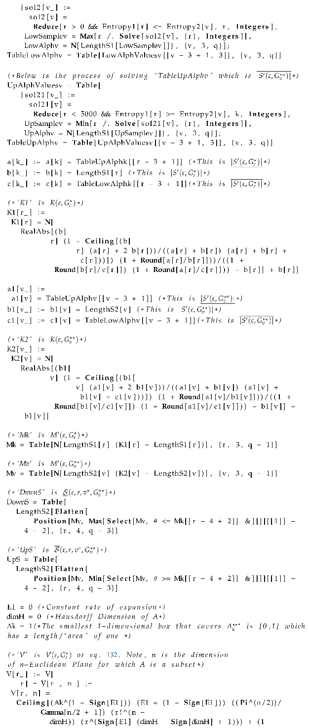
Hence, using $\left|{\mathcal{S}}^{\prime }\right|$, $\overline{\left|{\mathcal{S}}^{\prime }\right|}$, $\underline{\left|{\mathcal{S}}^{\prime }\right|}$, E, $\mathcal{E}(C,G_r^{★})$ (§5.4), and $T(C,G_r^{★})$, such that with the absolute value function $\left|\right|·\left|\right|$, ceiling function $\lceil ·\rceil$, and nearest integer function $\left[·\right]$, we define:

$$\begin{array}{cc}& K(\epsilon ,G_r^{★})=\hfill \\ & \left(1+\left|\left|E-\mathcal{E}(C,G_r^{★})\right|\right|\right)5\left(5\right|5|{\displaystyle \frac{\left|{\mathcal{S}}^{\prime }\right|\left(1+⌈\frac{\left|{\mathcal{S}}^{\prime }\right|\left(\underline{\left|{\mathcal{S}}^{\prime }\right|}+2\left|{\mathcal{S}}^{\prime }\right|\right)}{\left(\underline{\left|{\mathcal{S}}^{\prime }\right|}+\left|{\mathcal{S}}^{\prime }\right|\right)\left(\underline{\left|{\mathcal{S}}^{\prime }\right|}+\left|{\mathcal{S}}^{\prime }\right|+\overline{\left|{\mathcal{S}}^{\prime }\right|}\right)}⌉\right)\left(1+\left[\underline{\left|{\mathcal{S}}^{\prime }\right|}/\left|{\mathcal{S}}^{\prime }\right|\right]\right)}{\left(1+\left[\left|{\mathcal{S}}^{\prime }\right|/\overline{\left|{\mathcal{S}}^{\prime }\right|}\right]\right)\left(1+\left[\underline{\left|{\mathcal{S}}^{\prime }\right|}/\overline{\left|{\mathcal{S}}^{\prime }\right|}\right]\right)}}-\left|{\mathcal{S}}^{\prime }\right|5\left|5\right|+\left|{\mathcal{S}}^{\prime }\right|5)-T(C,G_r^{★})\mathcal{E}(C,G_r^{★})\hfill \end{array}$$

(128)

where $\mathcal{E}$, E, and T are “removed" when $\mathcal{E},E=0$, the choice function which answers the leading question in $\S$3.1 could be the following, s.t.we explain the reason behind choosing the choice function in §6.4:

Theorem 9. 

If we define:

$$\mathcal{M}(\epsilon ,G_r^{★})=\left|{\mathcal{S}}^{\prime }(\epsilon ,G_r^{★})\right|\left(K(\epsilon ,G_r^{★})-\left|{\mathcal{S}}^{\prime }(\epsilon ,G_r^{★})\right|\right)$$

$$\mathcal{M}(\epsilon ,G_v^{★★})=\left|{\mathcal{S}}^{\prime }(\epsilon ,G_v^{★★})\right|\left(K(\epsilon ,G_v^{★★})-\left|{\mathcal{S}}^{\prime }(\epsilon ,G_v^{★★})\right|\right)$$

where for $\mathcal{M}(\epsilon ,G_r^{★})$, we define $\mathcal{M}(\epsilon ,G_r^{★})$ to be the same as $\mathcal{M}(\epsilon ,G_v^{★★})$ when swapping “$v\in \mathbb{N}$" with “$r\in \mathbb{N}$" (for eq. 121 & 122) and sets $G_r^{★}$ with $G_v^{★★}$ (for eq. 121–128), then for constant $v>0$ and variable $v^{*}>0$, if:

$$\overline{\mathcal{S}}(\epsilon ,r,v^{*},G_v^{★★})=inf\left(\left\{|{\mathcal{S}}^{\prime }(\epsilon ,G_v^{★★})|:v\in \mathbb{N},\mathcal{M}(\epsilon ,G_v^{★★})\ge \mathcal{M}(\epsilon ,G_r^{★})\ge v^{*}\right\}\cup \left\{v^{*}\right\}\right)+v$$

(129)

and:

$$\underline{\mathcal{S}}(\epsilon ,r,v^{*},G_v^{★★})=sup\left(\left\{|{\mathcal{S}}^{\prime }(\epsilon ,G_v^{★★})|:v\in \mathbb{N},v^{*}\le \mathcal{M}(\epsilon ,G_v^{★★})\le \mathcal{M}(\epsilon ,G_r^{★})\right\}\cup \{-v^{*}\}\right)+v$$

(130)

where for all $r,v\in \mathbb{N}$, there exists a $f_r^{★}\in \mathcal{B}$ and $A_r^{★}\in \mathcal{B}$ ($\S$6.1 crit. 6.1), such for all $f_v^{★★}\in \mathbf{B}\left({\mathbb{R}}^A\right)\setminus \mathcal{B}$ and $A_v^{★★}\in \mathbf{B}\left(2^{{\mathbb{R}}^n}\right)\setminus \mathcal{B}$ ($\S$6.1 crit. 6.1), whenever:

$$inf\left\{\left|\right|1-c\left|\right|:\forall (ϵ>0)\exists (c>0)\forall (r\in \mathbb{N})\exists (v\in \mathbb{N})\left(\left|\left|{\displaystyle \frac{\left|{\mathcal{S}}^{\prime }(\epsilon ,G_r^{★})\right|}{\left|{\mathcal{S}}^{\prime }(\epsilon ,G_v^{★★})\right|}}-c\right|\right|<\epsilon \right)\right\}$$

(131)

such that $\lceil ·\rceil$ is the ceiling function, E is the fixed rate of expansion, Γ is the gamma function, n is the dimension of ${\mathbb{R}}^n$, ${\dim }_H\left(G_r^{★}\right)$ is the Hausdorff dimension of set $G_r^{★}\subseteq {\mathbb{R}}^{n+1}$, and ${\mathbf{A}}_r$ is area of the smallest $(n+1)$-dimensional box that contains $A_r^{★}$, then:

$$\begin{array}{cccc}\hfill & & & V(\epsilon ,G_r^{★},n)=\hfill \\ \hfill & \lceil \hfill & & ({\mathbf{A}}_{\mathbf{r}}^{1-\mathrm{sign}\left(E\right)}(E-\mathrm{sign}\left(E\right)+1)\left({\displaystyle \frac{exp\left(nln\left(\pi \right)/2\right)}{\Gamma (n/2+1)}}\right)\left({r!}^{(n-{\dim }_{\mathrm{H}}\left(G_r^{★}\right))}\right)\left(r^{\mathrm{sign}\left(E\right)\left({\dim }_{\mathrm{H}}\left(G_r^{★}\right)-\mathrm{sign}\left({\dim }_{\mathrm{H}}\left(G_r^{★}\right)\right)+1\right)}\right)+\hfill \\ & & & (1-\mathrm{sign}\left({\dim }_{\mathrm{H}}\left(G_r^{★}\right)\right)))/\epsilon \rceil /|{\mathcal{S}}^{\prime }(\epsilon ,G_r^{★})|\hfill \end{array}$$

(132)

& the choice function is:

$$\begin{array}{cccc}\hfill & \underset{\epsilon \to 0}{lim\; sup}\underset{v^{*}\to \infty }{lim}\underset{r\to \infty }{lim\; sup}\hfill & & \left({\displaystyle \frac{\mathrm{sign}\left(\mathcal{M}(\epsilon ,G_r^{★})\right)\overline{\mathcal{S}}(\epsilon ,r,v^{*},G_v^{★★})}{|{\mathcal{S}}^{\prime }(\epsilon ,G_r^{★})|+v}}-c^{-V(\epsilon ,G_r^{★},n)}\right)\hfill \\ & & & \left({\displaystyle \frac{\mathrm{sign}\left(\mathcal{M}(\epsilon ,G_r^{★})\right)\underline{\mathcal{S}}(\epsilon ,r,v^{*},G_v^{★★})}{|{\mathcal{S}}^{\prime }(\epsilon ,G_r^{★})|+v}}-c^{-V(\epsilon ,G_r^{★},n)}\right)=\hfill \end{array}$$

(133)

$$\begin{array}{cccc}& \underset{\epsilon \to 0}{lim\; inf}\underset{v^{*}\to \infty }{lim}\underset{r\to \infty }{lim\; inf}\hfill & & \left({\displaystyle \frac{\mathrm{sign}\left(\mathcal{M}(\epsilon ,G_r^{★})\right)\overline{\mathcal{S}}(\epsilon ,k,v^{*},G_v^{★★})}{|{\mathcal{S}}^{\prime }(\epsilon ,G_r^{★})|+v}}-c^{-V(\epsilon ,G_r^{★},n)}\right)\hfill \\ & & & \left({\displaystyle \frac{\mathrm{sign}\left(\mathcal{M}(\epsilon ,G_r^{★})\right)\underline{\mathcal{S}}(\epsilon ,r,v^{*},G_v^{★★})}{|{\mathcal{S}}^{\prime }(\epsilon ,G_r^{★})|+v}}-c^{-V(\epsilon ,G_r^{★},n)}\right)=0\hfill \end{array}$$

(134)

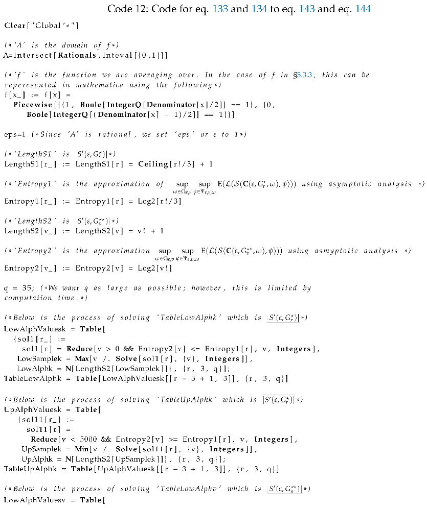
where ${\left(G_r^{★}\right)}_{k\in \mathbb{N}}$ satisfies eq. 133 & eq. . (Note, we want $sup\varnothing =-\infty$ and $inf\varnothing =+\infty$) s.t.the expected value which answers the approach of $\S$, using the leading question $\left(\S \right)$ is $\mathbb{E}\left[f_r^{★}\right]$

6.4. Explaining The Choice Function and Evidence The Choice Function Is Credible

Notice, before reading the programming in code 12, without the “c"-terms in eq. 133 and eq. 134:

(1)

The choice function in eq. 133 and eq. 134 is zero, when what I’m measuring from ${\left(G_r^{★}\right)}_{k\in \mathbb{N}}$ (§5.3.2 criteria 5.3.2) increases at a rate superlinear to that of ${\left(G_v^{★★}\right)}_{j\in \mathbb{N}}$, where $\mathrm{sign}\left(\mathcal{M}(\epsilon ,G_r^{★})\right)=0$.

(2)

The choice function in eq. 133 and eq. 134 is zero, when for a given ${\left(G_r^{★}\right)}_{k\in \mathbb{N}}$ and ${\left(G_v^{★★}\right)}_{j\in \mathbb{N}}$ there doesn’t exist c where eq. 131 is satisfied or $c=0$.

(3)

When c does exist, suppose:

$$\left\{\mathcal{J}\left(r\right):k\in \mathbb{N},{\displaystyle \frac{|{\mathcal{S}}^{\prime }(\epsilon ,G_r^{★})|}{|{\mathcal{S}}^{\prime }(\epsilon ,G_{\mathcal{J}\left(r\right)}^{★★})|}}\approx c\right\}$$

(135)

(a)

When $|{\mathcal{S}}^{\prime }(\epsilon ,G_r^{★})|<|{\mathcal{S}}^{\prime }(\epsilon ,G_{\mathcal{J}\left(r\right)}^{★★})|$, then:

$$\begin{array}{cc}\hfill & \underset{\epsilon \to 0}{lim\; sup}\underset{v^{*}\to \infty }{lim}\underset{r\to \infty }{lim\; sup}{\displaystyle \frac{\mathrm{sign}\left(\mathcal{M}(\epsilon ,G_r^{★})\right)\overline{\mathcal{S}}(\epsilon ,r,v^{*},G_v^{★★})}{|{\mathcal{S}}^{\prime }(\epsilon ,G_r^{★})|+v}}=c\hfill \end{array}$$

(136)

$$\begin{array}{cc}\hfill & \underset{\epsilon \to 0}{lim\; inf}\underset{v^{*}\to \infty }{lim}\underset{r\to \infty }{lim\; inf}{\displaystyle \frac{\mathrm{sign}\left(\mathcal{M}(\epsilon ,G_r^{★})\right)\underline{\mathcal{S}}(\epsilon ,r,v^{*},G_v^{★★})}{|{\mathcal{S}}^{\prime }(\epsilon ,G_r^{★})|+v}}=0\hfill \end{array}$$

(137)

(b)

When $|{\mathcal{S}}^{\prime }(\epsilon ,G_r^{★})|>|{\mathcal{S}}^{\prime }(\epsilon ,G_{\mathcal{J}\left(r\right)}^{★★})|$, then:

$$\begin{array}{cc}\hfill & \underset{\epsilon \to 0}{lim\; sup}\underset{v^{*}\to \infty }{lim}\underset{r\to \infty }{lim\; sup}{\displaystyle \frac{\mathrm{sign}\left(\mathcal{M}(\epsilon ,G_r^{★})\right)\overline{\mathcal{S}}(\epsilon ,k,v^{*},G_v^{★★})}{|{\mathcal{S}}^{\prime }(\epsilon ,G_r^{★})|+v}}=+\infty \hfill \end{array}$$

(138)

$$\begin{array}{cc}\hfill & \underset{\epsilon \to 0}{lim\; inf}\underset{v^{*}\to \infty }{lim}\underset{r\to \infty }{lim\; inf}{\displaystyle \frac{\mathrm{sign}\left(\mathcal{M}(\epsilon ,G_r^{★})\right)\underline{\mathcal{S}}(\epsilon ,k,v^{*},G_v^{★★})}{|{\mathcal{S}}^{\prime }(\epsilon ,G_r^{★})|+v}}=1/c\hfill \end{array}$$

(139)

Hence, for each sub-criteria under crit. (6.4), if we subtract one of their limits by their limit value, then eq. 133 and eq. 134 is zero. (We do this using the “c"-term in eq. 133 and 134). However, when the exponents of the “c"-terms aren’t equal to $-1$, the limits of eq. 133 and 134 aren’t equal to zero. We want this, infact, whenever we swap ${\mathcal{S}}^{\prime }(\epsilon ,G_r^{★})$ with ${\mathcal{S}}^{\prime }(\epsilon ,G_v^{★★})$. Moreover, we define function $V(\epsilon ,G_r^{★},n)$ (i.e., eq. 132), where:

(3)

(i)

When $S^{\prime }(\epsilon ,G_r^{★})\gg \mathrm{Numerator}\left(V(\epsilon ,G_r^{★},n)\right)$, then eq. 133 and 134 without the “c"-terms are zero. (The “c"-terms approach zero and still allow eq. 133 and 134 to equal zero.)

(ii)

When $S^{\prime }(\epsilon ,G_r^{★})\ll \mathrm{Numerator}\left(V(\epsilon ,G_r^{★},n)\right)$, then $\mathrm{sign}\left(\mathcal{M}(\epsilon ,G_r^{★})\right)$ is zero which makes eq. 133 and equal zero.

(iii)

Here are some examples of the numerator of $V(\epsilon ,G_r^{★},n)$ (eq. 132):

(A)

When $E=0$, $n=1$, and ${\dim }_H\left(A\right)=0$, the numerator of $V(\epsilon ,G_r^{★},n)$ is $\lceil \left(\mathbf{A}r!+1\right)/\epsilon \rceil$

(B)

When $E=z$, $n=1$, and ${\dim }_H\left(A\right)=0$, the numerator of $V(\epsilon ,G_r^{★},n)$ is $\lceil \left(2zr·r!+1\right)/\epsilon \rceil$

(C)

When $E=0$, $n=z_2$, and ${\dim }_H\left(A\right)=z_2$, the numerator of $V(\epsilon ,G_r^{★},n)$ is ceiling of constant $\mathbf{A}$ times the volume of an n-dimensional ball with finite radius: i.e.,

$$⌈{\displaystyle \frac{\mathbf{A}{z}_{1}exp\left(z_{2}ln\left(\pi \right)/2\right)}{\Gamma (z_2/2+1)}}/\epsilon ⌉$$

(D)

When $E=z_1$, $n=z_2$, and ${\dim }_H\left(A\right)=z_2$, the numerator of $V(\epsilon ,G_r^{★},n)$ is ceiling of the volume of the n-dimensional ball: i.e.,

$$⌈{\displaystyle \frac{z_{1}exp\left(z_{2}ln\left(\pi \right)/2\right)}{\Gamma (z_2/2+1)}}{r}^{z_2}/\epsilon ⌉$$

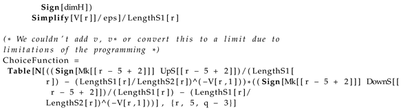
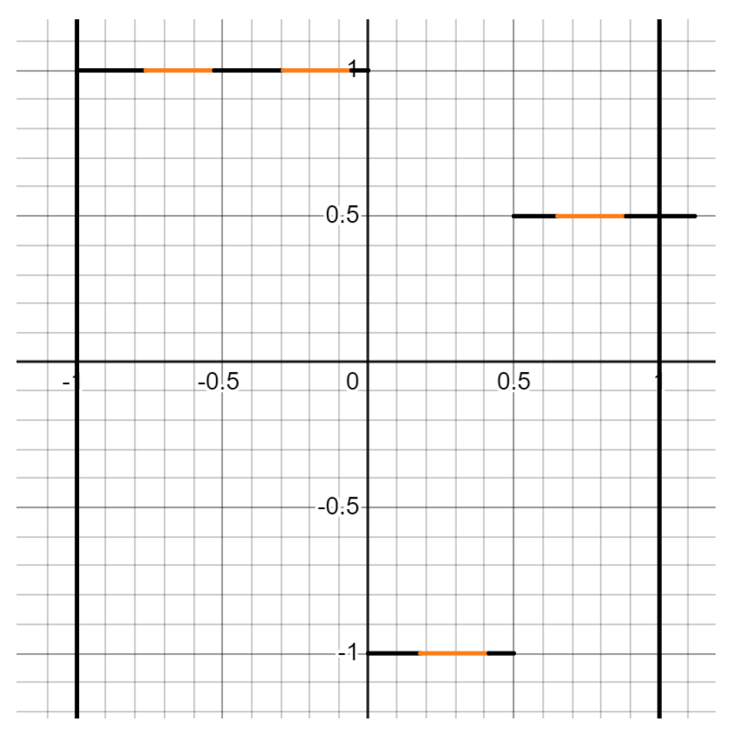
Now, consider the code for eq. 133 and eq. 134. (Note, the set theoretic limit of $G_r^{★}$ is the graph of function $f:A\to \mathbb{R}$.) In this example, $A=\mathbb{Q}\cap [0,1]$, and:

$$f\left(x\right)=\left\{\begin{array}{cc}1\hfill & x\in \left\{(2s+1)/\left(2t\right):s\in \mathbb{Z},t\in \mathbb{N},t\ne 0\right\}\cap [0,1]\hfill \\ 0\hfill & x\notin \left\{(2s+1)/\left(2t\right):s\in \mathbb{Z},t\in \mathbb{N},t\ne 0\right\}\cap [0,1]\hfill \end{array}\right.$$

(140)

such that:

$${\left(A_r^{★}\right)}_{r\in \mathbb{N}}={\left(\left\{c/(r!):c\in \mathbb{Z},0\le c\le r!\right\}\right)}_{r\in \mathbb{N}}$$

the ceiling function is $\lceil ·\rceil$, and:

$${\left(A_v^{★★}\right)}_{v\in \mathbb{N}}={\left(\left\{c/\lceil v!/3\rceil :c\in \mathbb{Z},0\le c\le \lceil v!/3\rceil \right\}\right)}_{v\in \mathbb{N}}$$

such for $f_r^{★}:A_r^{★}\to \mathbb{R}$,

$$f_r^{★}\left(x\right)=f\left(x\right)\mathrm{for}\mathrm{all}x\in A_r^{★}$$

(141)

and $f_v^{★★}:A_v^{★★}\to \mathbb{R}$

$$f_v^{★★}\left(x\right)=f\left(x\right)\mathrm{for}\mathrm{all}x\in A_v^{★★}$$

(142)

Hence, when ${\left(G_r^{★}\right)}_{r\in \mathbb{N}}$ is:

$${\left(G_r^{★}\right)}_{r\in \mathbb{N}}={\left(\left\{(x,f\left(x\right)):x\in \left\{c/k!:c\in \mathbb{Z},0\le c\le k!\right\}\right\}\right)}_{r\in \mathbb{N}}$$

(143)

and ${\left(G_v^{★★}\right)}_{v\in \mathbb{N}}$ is:

$${\left(G_v^{★★}\right)}_{v\in \mathbb{N}}={\left(\left\{(x,f\left(x\right)):x\in \left\{c/\lceil v!/3\rceil :c\in \mathbb{Z},0\le c\le \lceil v!/3\rceil \right\}\right\}\right)}_{v\in \mathbb{N}}$$

(144)

Note, the following (we leave this to mathematicians to figure LengthS1, LengthS2, Entropy1 and $\mathtt{Entropy}\mathtt{2}$ for other A and f in code 12).

6.4.1. Evidence With Programming

7. Questions

(1)

Does $\S$ answer the $\mathbf{leading}\mathbf{question}$ in $\S$

(2)

Using thm. 9, when f is defined in $\S$, does $\mathbb{E}\left[f_r^{★}\right]$ have a finite value?

(3)

Using thm. 9, when f is defined in $\S$, does $\mathbb{E}\left[f_r^{★}\right]$ have a finite value?

(4)

If there’s no time to check questions i, ii and iii, see $\S$.

8. Appendix of §5.3.1

8.1 Example of §5.3.1, step 5.3.1

Suppose

(1)

$A=\mathbb{R}$

(2)

When defining $f:A\to \mathbb{R}$:

$$f\left(x\right)=\left\{\begin{array}{cc}1\hfill & x<0\hfill \\ -1\hfill & 0\le x<0.5\hfill \\ 0.5\hfill & 0.5\le x\hfill \end{array}\right.$$

(145)

(3)

${\left(G_r^{★}\right)}_{r\in \mathbb{N}}={\left(\left\{(x,f(x\left)\right):-r\le x\le r\right\}\right)}_{r\in \mathbb{N}}$

Then one example of $\mathbf{C}(\sqrt{2}/6,G_1^{★},1)$, using §5.3.1 step 1, (where $G_1^{★}={\left(\left\{(x,f(x\left)\right):-1\le x\le 1\right\}\right)}_{r\in \mathbb{N}}$) is:

$$\begin{array}{cccc}& \{\hfill & & \left\{(x,f\left(x\right)):-1\le x\le {\displaystyle \frac{\sqrt{2}-6}{6}}\right\},\left\{(x,f\left(x\right)):{\displaystyle \frac{\sqrt{2}-6}{6}}\le x\le {\displaystyle \frac{2\sqrt{2}-6}{6}}\right\},\left\{(x,f\left(x\right)):{\displaystyle \frac{2\sqrt{2}-6}{6}}\le x\le {\displaystyle \frac{3\sqrt{2}-6}{6}}\right\}\hfill \\ & & & \left\{(x,f\left(x\right)):{\displaystyle \frac{3\sqrt{2}-6}{6}}\le x\le {\displaystyle \frac{4\sqrt{2}-6}{6}}\right\},\left\{(x,f\left(x\right)):{\displaystyle \frac{4\sqrt{2}-6}{6}}\le x\le {\displaystyle \frac{5\sqrt{2}-6}{6}}\right\},\left\{(x,f\left(x\right)):{\displaystyle \frac{5\sqrt{2}-6}{6}}\le x\le {\displaystyle \frac{6\sqrt{2}-6}{6}}\right\}\hfill \\ & & & \left\{(x,f\left(x\right)):{\displaystyle \frac{6\sqrt{2}-6}{6}}\le x\le {\displaystyle \frac{7\sqrt{2}-6}{6}}\right\},\left\{(x,f\left(x\right)):{\displaystyle \frac{7\sqrt{2}-6}{6}}\le x\le {\displaystyle \frac{8\sqrt{2}-6}{6}}\right\},\left\{(x,f\left(x\right)):{\displaystyle \frac{8\sqrt{2}-6}{6}}\le x\le {\displaystyle \frac{9\sqrt{2}-6}{6}}\right\}\}\hfill \end{array}$$

(146)

Note, the length of each partition is $\sqrt{2}/6$, where the borders could be approximated as:

$$\begin{array}{cccc}& \{\hfill & & \left\{(x,f(x\left)\right):-1\le x\le -.764\right\},\left\{(x,f(x\left)\right):-.764\le x\le -.528\right\},\left\{(x,f(x\left)\right):-.528\le x\le -.293\right\}\hfill \\ & & & \left\{(x,f(x\left)\right):-.293\le x\le -.057\right\},\left\{(x,f(x\left)\right):-.057\le x\le .178\right\},\left\{(x,f(x\left)\right):.178\le x\le .414\right\}\hfill \\ & & & \left\{(x,f(x\left)\right):.414\le x\le .65\right\},\left\{(x,f(x\left)\right):.65\le x\le .886\right\},\left\{(x,f(x\left)\right):.886\le x\le 1.121\right\}\}\hfill \end{array}$$

(147)

which is illustrated using alternating orange/black lines of equal length covering $G_1^{★}$ (i.e., the black vertical lines are the smallest and largest x-cooridinates of $G_1^{★}$).

(Note, the alternating covers in Figure 3 satisfy step (1) of §5.3.1, because the Hausdorff measure in its dimension of the covers is $\sqrt{2}/6$ and there are 9 covers over-covering $G_1^{★}$: i.e.,

Figure 3. The alternating orange & black lines are the “covers" and the vertical lines are the boundaries of $G_1^{★}$.

Figure 3. The alternating orange & black lines are the “covers" and the vertical lines are the boundaries of $G_1^{★}$.

Definition 

(Minimum Covers of Measure $\epsilon =\sqrt{2}/6$ covering $G_1^{★}$). We can compute the minimum covers of $\mathbf{C}(\sqrt{2}/6,G_1^{★},1)$, using the formula:

$$\lceil {\mathcal{H}}^{{\dim }_{\mathrm{H}}\left(G_1^{★}\right)}\left(G_1^{★}\right)/(\sqrt{2}/6)\rceil$$

where $\lceil {\mathcal{H}}^{{\dim }_{\mathrm{H}}\left(G_1^{★}\right)}\left(G_1^{★}\right)/(\sqrt{2}/6)\rceil =\lceil \mathrm{Length}\left([-1,1]\right)/(\sqrt{2}/6)\rceil =\lceil 2/(\sqrt{2}/6)\rceil =\lceil 6\sqrt{2}\rceil =\lceil 6\left(1.4\right)\rceil =\lceil 8+.4\rceil =9$).

Note there are other examples of $\mathbf{C}(\sqrt{2}/6,G_1^{★},\omega )$ for different $\omega$. Here is another case:

which can be defined (see eq. 146 for comparison):

$$\begin{array}{cccc}& \{\hfill & & \left\{(x,f\left(x\right)):{\displaystyle \frac{6-9\sqrt{2}}{6}}\le x\le {\displaystyle \frac{6-8\sqrt{2}}{6}}\right\},\left\{(x,f\left(x\right)):{\displaystyle \frac{6-8\sqrt{2}}{6}}\le x\le {\displaystyle \frac{6-7\sqrt{2}}{6}}\right\},\left\{(x,f\left(x\right)):{\displaystyle \frac{6-7\sqrt{2}}{6}}\le x\le {\displaystyle \frac{6-6\sqrt{2}}{6}}\right\}\hfill \\ & & & \left\{(x,f\left(x\right)):{\displaystyle \frac{6-6\sqrt{2}}{6}}\le x\le {\displaystyle \frac{6-5\sqrt{2}}{6}}\right\},\left\{(x,f\left(x\right)):{\displaystyle \frac{6-5\sqrt{2}}{6}}\le x\le {\displaystyle \frac{6-4\sqrt{2}}{6}}\right\},\left\{(x,f\left(x\right)):{\displaystyle \frac{6-4\sqrt{2}}{6}}\le x\le {\displaystyle \frac{6-3\sqrt{2}}{6}}\right\}\hfill \\ & & & \left\{(x,f\left(x\right)):{\displaystyle \frac{6-3\sqrt{2}}{6}}\le x\le {\displaystyle \frac{6-2\sqrt{2}}{6}}\right\},\left\{(x,f\left(x\right)):{\displaystyle \frac{6-2\sqrt{2}}{6}}\le x\le {\displaystyle \frac{6-\sqrt{2}}{6}}\right\},\left\{(x,f\left(x\right)):{\displaystyle \frac{6-\sqrt{2}}{6}}\le x\le 1\right\}\}\hfill \end{array}$$

(148)

In the case of $G_1^{★}$, there are uncountable different covers$\mathbf{C}(\sqrt{2}/6,G_1^{★},\omega )$ which can be used. For instance, when $0\le \alpha \le (12-9\sqrt{2})/6$ (i.e., $\omega =\alpha -(12-9\sqrt{2})/6+1$) consider:

$$\begin{array}{cccc}& \{\hfill & & \left\{(x,f\left(x\right)):\alpha -1+\alpha \le x\le \alpha +{\displaystyle \frac{\sqrt{2}-6}{6}}\right\},\left\{(x,f\left(x\right)):\alpha +{\displaystyle \frac{\sqrt{2}-6}{6}}\le x\le \alpha +{\displaystyle \frac{2\sqrt{2}-6}{6}}\right\},\left\{(x,f\left(x\right)):\alpha +{\displaystyle \frac{2\sqrt{2}-6}{6}}\le x\le \alpha +{\displaystyle \frac{3\sqrt{2}-6}{6}}\right\}\hfill \\ & & & \left\{(x,f\left(x\right)):\alpha +{\displaystyle \frac{3\sqrt{2}-6}{6}}\le x\le \alpha +{\displaystyle \frac{4\sqrt{2}-6}{6}}\right\},\left\{(x,f\left(x\right)):\alpha +{\displaystyle \frac{4\sqrt{2}-6}{6}}\le x\le \alpha +{\displaystyle \frac{5\sqrt{2}-6}{6}}\right\},\hfill \\ & & & \left\{(x,f\left(x\right)):\alpha +{\displaystyle \frac{5\sqrt{2}-6}{6}}\le x\le \alpha +{\displaystyle \frac{6\sqrt{2}-6}{6}}\right\},\left\{(x,f\left(x\right)):\alpha +{\displaystyle \frac{6\sqrt{2}-6}{6}}\le x\le \alpha +{\displaystyle \frac{7\sqrt{2}-6}{6}}\right\}\hfill \\ & & & \left\{(x,f\left(x\right)):\alpha +{\displaystyle \frac{7\sqrt{2}-6}{6}}\le x\le \alpha +{\displaystyle \frac{8\sqrt{2}-6}{6}}\right\},\left\{(x,f\left(x\right)):\alpha +{\displaystyle \frac{8\sqrt{2}-6}{6}}\le x\le \alpha +{\displaystyle \frac{9\sqrt{2}-6}{6}}\right\}\}\hfill \end{array}$$

(149)

When $\alpha =0$ and $\omega =(9\sqrt{2}-6)/6$, we get Figure 4 and when $\alpha =(12-9\sqrt{2})/6$ and $\omega =1$, we get Figure 3

Figure 4. This is similar to Figure 3, except the start-points of the covers are shifted all the way to the left.

Figure 4. This is similar to Figure 3, except the start-points of the covers are shifted all the way to the left.

8.2. Example of §5.3.1, Step 5.3.1. Suppose:

(1)

$A=\mathbb{R}$

(2)

When defining $f:A\to \mathbb{R}$: i.e.,

$$f\left(x\right)=\left\{\begin{array}{cc}1\hfill & x<0\hfill \\ -1\hfill & 0\le x<0.5\hfill \\ 0.5\hfill & 0.5\le x\hfill \end{array}\right.$$

(150)

(3)

${\left(G_r^{★}\right)}_{r\in \mathbb{N}}={\left(\left\{(x,f(x\left)\right):-r\le x\le r\right\}\right)}_{r\in \mathbb{N}}$

(4)

$G_1^{★}=\left\{(x,f(x\left)\right):-1\le x\le 1\right\}$

(5)

$\mathbf{C}(\sqrt{2}/6,G_1^{★},1)$, using eq. 147 and Figure 3, which is approximately

$$\begin{array}{cccc}& \{\hfill & & \left\{(x,f(x\left)\right):-1\le x\le -.764\right\},\left\{(x,f(x\left)\right):-.764\le x\le -.528\right\},\left\{(x,f(x\left)\right):-.528\le x\le -.293\right\}\hfill \\ & & & \left\{(x,f(x\left)\right):-.293\le x\le -.057\right\},\left\{(x,f(x\left)\right):-.057\le x\le .178\right\},\left\{(x,f(x\left)\right):.178\le x\le .414\right\}\hfill \\ & & & \left\{(x,f(x\left)\right):.414\le x\le .65\right\},\left\{(x,f(x\left)\right):.65\le x\le .886\right\},\left\{(x,f(x\left)\right):.886\le x\le 1.121\right\}\}\hfill \end{array}$$

(151)

Then, an example of $\mathcal{S}(\mathbf{C}(\sqrt{2}/6,G_1^{★},1),1)$ is:

$$\left\{\right(-.9,1),(-.65,1),(-.4,1),(-.2,1),(.1,-1),(.3,-1),(.55,.5),(.75,.5),(1,.5\left)\right\}$$

(152)

Below, we illustrate the sample: i.e., the set of all blue points in each orange and black line of $\mathbf{C}(\sqrt{2}/6,G_1^{★},1)$ covering $G_1^{★}$:

Figure 5. The blue points are the “sample points", the alternative black and orange lines are the “covers", and the red lines are the smallest & largest x-coordinates $G_1^{★}$.

Figure 5. The blue points are the “sample points", the alternative black and orange lines are the “covers", and the red lines are the smallest & largest x-coordinates $G_1^{★}$.

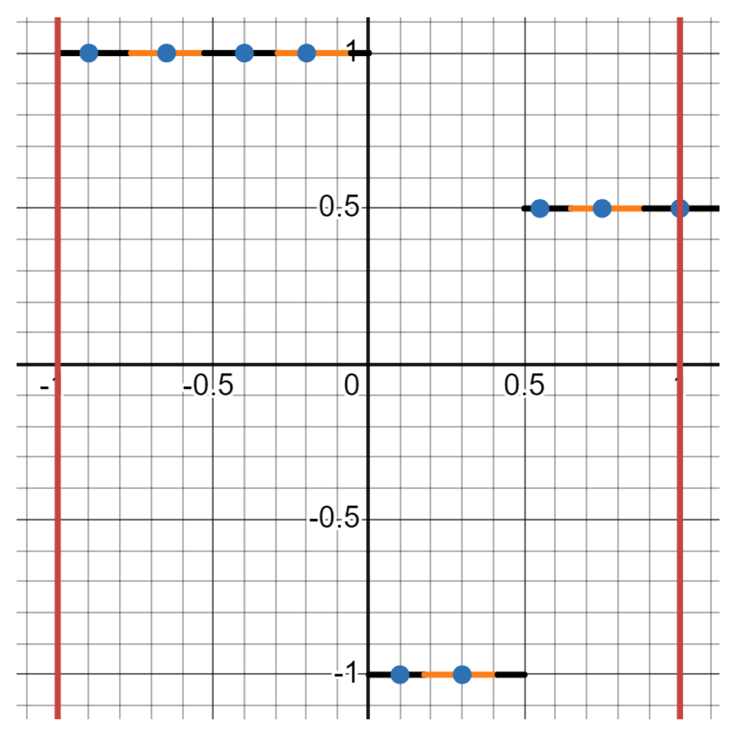
Note, there are multiple samples that can be taken, as long as one sample point is taken from each cover in $\mathbf{C}(\sqrt{2}/6,G_1^{★},1)$.

8.3. Example of §5.3.1, Step 5.3.1 Suppose

(1)

$A=\mathbb{R}$

(2)

When defining $f:A\to \mathbb{R}$:

$$f\left(x\right)=\left\{\begin{array}{cc}1\hfill & x<0\hfill \\ -1\hfill & 0\le x<0.5\hfill \\ 0.5\hfill & 0.5\le x\hfill \end{array}\right.$$

(153)

(3)

${\left(G_r^{★}\right)}_{r\in \mathbb{N}}={\left(\left\{(x,f(x\left)\right):-r\le x\le r\right\}\right)}_{r\in \mathbb{N}}$

(4)

$G_1^{★}=\left\{(x,f(x\left)\right):-1\le x\le 1\right\}$

(5)

$\mathbf{C}(\sqrt{2}/6,G_1^{★},1)$, using eq. 147 and Figure 3, is approx.

$$\begin{array}{cccc}& \{\hfill & & \left\{(x,f(x\left)\right):-1\le x\le -.764\right\},\left\{(x,f(x\left)\right):-.764\le x\le -.528\right\},\left\{(x,f(x\left)\right):-.528\le x\le -.293\right\}\hfill \\ & & & \left\{(x,f(x\left)\right):-.293\le x\le -.057\right\},\left\{(x,f(x\left)\right):-.057\le x\le .178\right\},\left\{(x,f(x\left)\right):.178\le x\le .414\right\}\hfill \\ & & & \left\{(x,f(x\left)\right):.414\le x\le .65\right\},\left\{(x,f(x\left)\right):.65\le x\le .886\right\},\left\{(x,f(x\left)\right):.886\le x\le 1.121\right\}\}\hfill \end{array}$$

(154)

(6)

$\mathcal{S}(\mathbf{C}(13/6,G_1^{★},1),1)$, using eq. 152, is:

$$\left\{\right(-.9,1),(-.65,1),(-.4,1),(-.2,1),(.1,-1),(.3,-1),(.55,.5),(.75,.5),(1,.5\left)\right\}$$

(155)

Therefore, consider the following process:

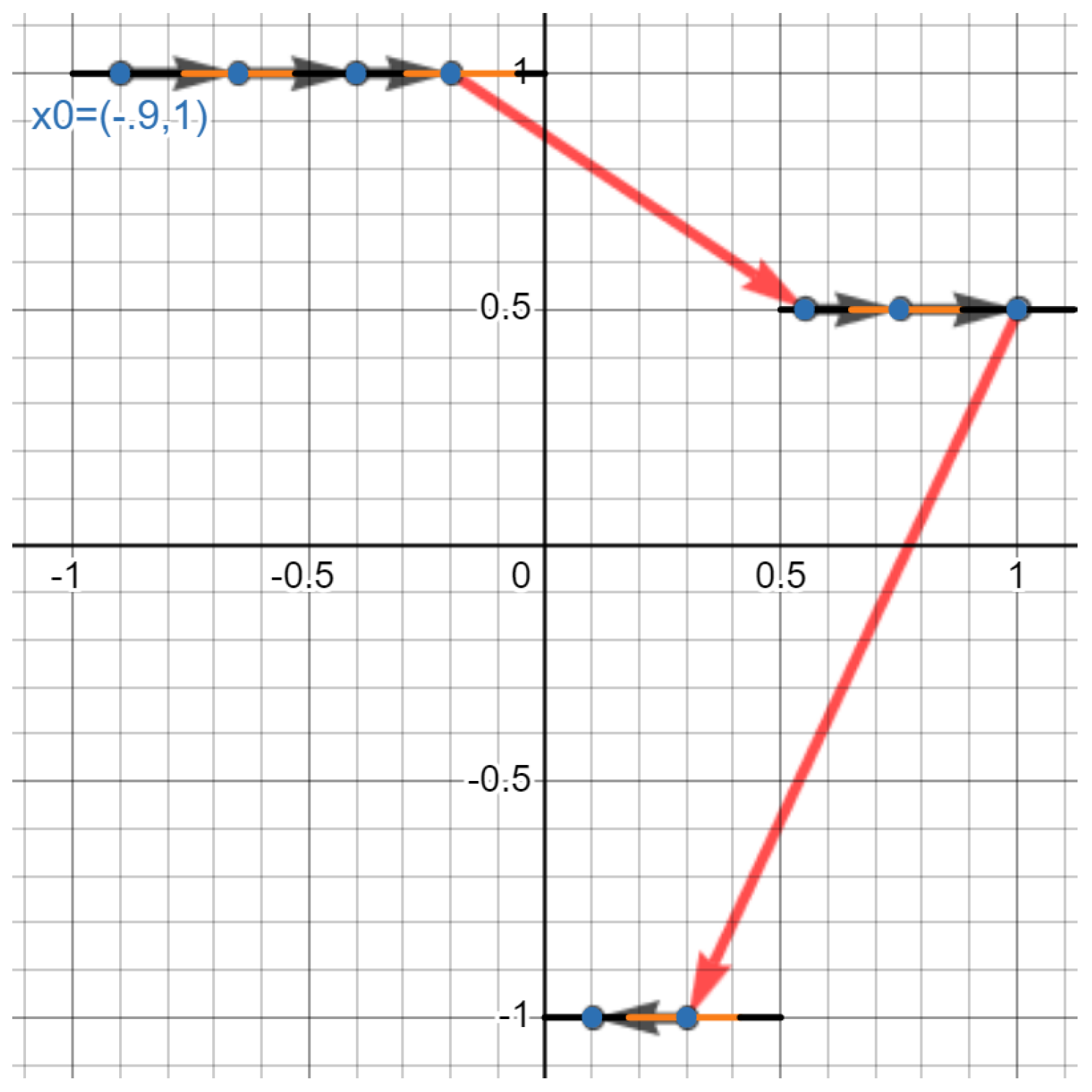
8.3.1. Step 5.3.10a

If $\mathcal{S}(\mathbf{C}(\sqrt{2}/6,G_1^{★},1),1)$ is:

$$\left\{\right(-.9,1),(-.65,1),(-.4,1),(-.2,1),(.1,-1),(.3,-1),(.55,.5),(.75,.5),(1,.5\left)\right\}$$

(156)

suppose $x_0=(-.9,1)$. Note, the following:

(1)

$x_1=(-.65,1)$ is the next point in the “pathway" since it’s a point in $\mathcal{S}(\mathbf{C}(\sqrt{2}/6,G_1^{★},1),1)$ with the smallest 2-d Euclidean distance to $x_0$ instead of $x_0$.

(2)

$x_2=(-.4,1)$ is the third point since it’s a point in $\mathcal{S}(\mathbf{C}(\sqrt{2}/6,G_1^{★},1),1)$ with the smallest 2-d Euclidean distance to $x_1$ instead of $x_0$ and $x_1$.

(3)

$x_3=(-.2,1)$ is the fourth point since it’s a point in $\mathcal{S}(\mathbf{C}(\sqrt{2}/6,G_1^{★},1),1)$ with the smallest 2-d Euclidean distance to $x_2$ instead of $x_0$, $x_1$, and $x_2$.

(4)

we continue this process, where the “pathway" of $\mathcal{S}(\mathbf{C}(\sqrt{2}/6,G_1^{★},1),1)$ is:

$$(-.9,1)\to (-.65,1)\to (-.4,1)\to (-.2,1)\to (.55,.5)\to (.75,.5)\to (1,.5)\to (.3,-1)\to (.1,-1)$$

(157)

Note 10. 

If more than one point has the minimum 2-d Euclidean distance from $x_0$, $x_1$, $x_2$, etc. take all potential pathways: e.g., using the sample in eq. 156, if $x_0=(-.65,1)$, then since $(-.9,1)$ and $(-.4,1)$ have the smallest Euclidean distance to $(-.65,1)$, taketwopathways:

$$(-.65,1)\to (-.9,1)\to (-.4,1)\to (-.2,1)\to (.55,.5)\to (.75,.5)\to (1,.5)\to (.3,-1)\to (.1,-1)$$

and also:

$$(-.65,1)\to (-.4,1)\to (-.2,1)\to (-.9,1)\to (.55,.5)\to (.75,.5)\to (1,.5)\to (.3,-1)\to (.1,-1)$$

8.3.2. Step 5.3.10b

Next, take the length of all line segments in each pathway. In other words, suppose $d(P,Q)$ is the n-th dim.Euclidean distance between points $P,Q\in {\mathbb{R}}^n$. Using the pathway in eq. 157, we want:

$$\begin{array}{cc}\hfill \{& d\left(\right(-.9,1),(-.65,1\left)\right),d\left(\right(-.65,1),(-.4,1\left)\right),d\left(\right(-.4,1),(-.2,1\left)\right),d\left(\right(-.2,1),(.55,.5\left)\right),\hfill \\ & d\left(\right(.55,.5),(.75,.5\left)\right),d\left(\right(.75,.5),(1,.5\left)\right),d\left(\right(1,.5),(.3,-1\left)\right),d\left(\right(.3,-1),(.1,-1\left)\right)\}\hfill \end{array}$$

(158)

Whose distances can be approximated as:

$$\begin{array}{cc}\hfill \{& .25,.25,.2,.901389,.2,.25,1.655295,.2\}\hfill \end{array}$$

Also, we see the outliers [6] are $.901389$ and $1.655295$ (i.e., notice that the outliers are more prominent for $\epsilon \ll \sqrt{2}/6$). Therefore, remove $.901389$ and $1.655295$ from our set of lengths:

$$\begin{array}{cc}\hfill \{& .25,.25,.2,.2,.25,.2\}\hfill \end{array}$$

This is illustrated using:

Figure 6. The black arrows are the “pathways" whose lengths aren’t outliers. The length of the red arrows in the pathway are outliers.

Figure 6. The black arrows are the “pathways" whose lengths aren’t outliers. The length of the red arrows in the pathway are outliers.

Hence, when $x_0=(-.9,1)$, using §5.3.1 step 33b & eq. 156, we note:

$$\mathcal{L}((-.9,1),\mathcal{S}(\mathbf{C}(\sqrt{2}/6,G_1^{★},1),1))=\{.25,.25,.2,.2,.25,.2\}$$

(159)

8.3.3. Step 5.3.10c

To convert the set of distances in eq. 159 into a probability distribution, we take:

$$\sum _{x\in \{.25,.25,.2,.2,.25,.2\}}x=.25+.25+.2+.2+.25+.2=1.35$$

(160)

Then divide each element in $\{.25,.25,.2,.2,.25,.2\}$ by 1.35

$$\{.25/(1.35),.25/(1.35),.2/(1.35),.2/(1.35),.25/(1.35),.2/(1.35\left)\right\}$$

which gives us the probability distribution:

$$\{5/27,5/27,4/27,4/27,5/27,4/27\}$$

Hence,

$$\mathbb{P}\left(\mathcal{L}((-.9,1),\mathcal{S}(\mathbf{C}(\sqrt{2}/6,G_1^{★},1),1))\right)=\{5/27,5/27,4/27,4/27,5/27,4/27\}$$

(161)

8.3.4. Step 5.3.10d

Take the shannon entropy of eq. 161:

$$\begin{array}{cc}\hfill & \mathrm{E}\left(\mathbb{P}\left(\mathcal{L}((-.9,1),\mathcal{S}(\mathbf{C}(\sqrt{2}/6,G_1^{★},1),1))\right)\right)=\hfill \\ & \sum _{x\in \mathbb{P}\left(\mathcal{L}((-.9,1),\mathcal{S}(\mathbf{C}(\sqrt{2}/6,G_1^{★},1),1))\right)}-x{log}_{2}x=\sum _{x\in \{5/27,5/27,4/27,4/27,5/27,4/27\}}-x{log}_{2}x=\hfill \\ & -(5/27){log}_2(5/27)-(5/27){log}_2(5/27)-(4/27){log}_2(4/27)-(4/27){log}_2(4/27)-(5/27){log}_2(5/27)-(4/27){log}_2(5/27)=\hfill \\ & -(15/27){log}_2(5/27)-(12/27){log}_2(4/27)\approx 2.57604\hfill \end{array}$$

We shorten $\mathrm{E}\left(\mathbb{P}\left(\mathcal{L}((-.9,1),\mathcal{S}(\mathbf{C}(\sqrt{2}/6,G_1^{★},1),1))\right)\right)$ to $\mathrm{E}\left(\mathcal{L}((-.9,1),\mathcal{S}(\mathbf{C}(\sqrt{2}/6,G_1^{★},1),1))\right)$, giving us:

$$\mathrm{E}\left(\mathcal{L}((-.9,1),\mathcal{S}(\mathbf{C}(\sqrt{2}/6,G_1^{★},1),1))\right)\approx 2.57604$$

(162)

8.3.5. Step 5.3.10e

Take the entropy, w.r.t all pathways, of the sample:

$$\left\{\right(-.9,1),(-.65,1),(-.4,1),(-.2,1),(.1,-1),(.3,-1),(.55,.5),(.75,.5),(1,.5\left)\right\}$$

(163)

In other words, we’ll compute:

$$\mathrm{E}\left(\mathcal{L}\left(\mathcal{S}(\mathbf{C}(\sqrt{2}/6,G_1^{★},1),1)\right)\right)=\underset{x_0\in \mathcal{S}(\mathbf{C}(\sqrt{2}/6,G_1^{★},1),1)}{sup}\mathrm{E}\left(\mathcal{L}(x_0,\mathcal{S}(\mathbf{C}(\sqrt{2}/6,G_1^{★},1),1))\right)$$

We do this by repeating §8.3.1-§8.3.4 for different $x_0\in \mathcal{S}(\mathbf{C}(\sqrt{2}/6,G_1^{★},1),1)\left)\right)$ (i.e., in the equation with multiple values, see note 10)

$$\begin{array}{cc}\hfill & \mathrm{E}\left(\mathcal{L}((-.9,1),\mathcal{S}(\mathbf{C}(\sqrt{2}/6,G_1^{★},1),1))\right)\approx 2.57604\hfill \end{array}$$

(164)

$$\begin{array}{cc}\hfill & \mathrm{E}\left(\mathcal{L}((-.65,1),\mathcal{S}(\mathbf{C}(\sqrt{2}/6,G_1^{★},1),1))\right)\approx 2.3131,2.377604\hfill \end{array}$$

(165)

$$\begin{array}{cc}\hfill & \mathrm{E}\left(\mathcal{L}((-.4,1),\mathcal{S}(\mathbf{C}(\sqrt{2}/6,G_1^{★},1),1))\right)\approx 2.3131\hfill \end{array}$$

(166)

$$\begin{array}{cc}\hfill & \mathrm{E}\left(\mathcal{L}((-.2,-1),\mathcal{S}(\mathbf{C}(\sqrt{2}/6,G_1^{★},1),1))\right)\approx 2.57604\hfill \end{array}$$

(167)

$$\begin{array}{cc}\hfill & \mathrm{E}\left(\mathcal{L}((-.1,-1),\mathcal{S}(\mathbf{C}(\sqrt{2}/6,G_1^{★},1),1))\right)\approx 1.86094\hfill \end{array}$$

(168)

$$\begin{array}{cc}\hfill & \mathrm{E}\left(\mathcal{L}((-.3,-1),\mathcal{S}(\mathbf{C}(\sqrt{2}/6,G_1^{★},1),1))\right)\approx 1.85289\hfill \end{array}$$

(169)

$$\begin{array}{cc}\hfill & \mathrm{E}\left(\mathcal{L}((.55,.5),\mathcal{S}(\mathbf{C}(\sqrt{2}/6,G_1^{★},1),1))\right)\approx 2.08327\hfill \end{array}$$

(170)

$$\begin{array}{cc}\hfill & \mathrm{E}\left(\mathcal{L}((.75,.5),\mathcal{S}(\mathbf{C}(\sqrt{2}/6,G_1^{★},1),1))\right)\approx 2.31185\hfill \end{array}$$

(171)

$$\begin{array}{cc}\hfill & \mathrm{E}\left(\mathcal{L}((1,.5),\mathcal{S}(\mathbf{C}(\sqrt{2}/6,G_1^{★},1),1))\right)\approx 2.2622\hfill \end{array}$$

(172)

Hence, since the largest value out of eq. 164-172 is $2.57604$:

$$\mathrm{E}\left(\mathcal{L}\left(\mathcal{S}(\mathbf{C}(13/6,G_1^{★},1),1)\right)\right)=\underset{x_0\in \mathcal{S}(\mathbf{C}(\epsilon ,G_1^{★},3),1)}{sup}\mathrm{E}\left(\mathcal{L}(x_0,\mathcal{S}(\mathbf{C}(\epsilon ,G_1^{★},1),1))\right)\approx 2.57604$$