New Algorithm for Entanglement Swapping

Zhaoxu Ji; Huanguo Zhang

doi:10.20944/preprints202502.1244.v2

Preprint

Article

New Algorithm for Entanglement Swapping

This version is not peer-reviewed.

This version is not peer-reviewed.

Downloads

Views

154

Comments

Submitted:

18 March 2025

Posted:

18 March 2025

You are already at the latest version

Abstract

Entanglement swapping is a key technology to realize long-distance quantum communication and build quantum networks, and has extensive and important applications in quantum information processing. In this paper, we propose a new algorithm to obtain entanglement swapping results, which is based on the idea of constructing new entangled states after entanglement swapping from all possible observation outcomes. We demonstrate the algorithm by the entanglement swapping between two bipartite entangled states, and derive the results of entanglement swapping between two 2-level Bell states, which are consistent with those obtained through algebraic calculations. Our work can provide new perspectives for thinking about the principles of quantum mechanics and trigger in-depth exploration of quantum mechanics principles and natural mysteries.

Keywords:

quantum entanglement

;

entanglement swapping

;

Bell states

;

quantum information processing

Subject:

Physical Sciences - Quantum Science and Technology

This preprints belongs to the Topic

Quantum Information and Quantum Computing, 2nd Volume

1. Introduction

Quantum superposition, or superposition for short, is a peculiar quantum mechanics phenomenon, which indicates that a quantum system can be in multiple different states simultaneously [1]. The most common case is the superposition of two opposing states, and one of the most famous examples is “Schr

\ddot{o}

dinger’s cat”, which can be vividly expressed as “a cat can be both alive and dead at the same time” [2].

Quantum entanglement, abbreviated as entanglement, is a quantum mechanics phenomenon built on superposition. In other words, the primary premise for the existence of entanglement is superposition. An entangled system is a composite of two or more subsystems, and if one of the subsystems is observed, the state of the other subsystems will change immediately without any time delay [1]. In a entangled state, the properties of each particle have been integrated into a whole property, and it is impossible to describe the properties of each particle separately, only the properties of the whole system can be described [1,3].

Entanglement swapping is another quantum mechanics phenomenon, which builds on entanglement. Entanglement swapping has attracted extensive attention in the academic community since its discovery, mainly because it is one of the core resources for preparing quantum repeaters, which makes long-distance quantum communication and and large-scale quantum networks possible [3,4,5]. In addition, entanglement swapping provides a new approach for the preparation of entangled states and is also an important resource for designing quantum cryptography protocols and quantum algorithms [5,6].

The original idea of entanglement swapping was included in the quantum teleportation scheme proposed by Bennett et al. in 1992 [7]. Subsequently, Zeilinger et al. experimentally realised entanglement swapping for the first time in 1993, and formally proposed the concept of entanglement swapping [4]. Bose et al. described the entanglement swapping of 2-level cat states [8]. Hardy and Song considered the entanglement swapping of general pure states [9]. Bouda and Bu

\overset{ˇ}{z}

ek generalized the entanglement swapping scheme originally proposed for two pairs of qubits to multi-qudit systems [10]. Karimipour et al. introduced generalized cat states for d-level systems and obtain the formulas for their entanglement swapping with generalized Bell states [11]. Sen et al. investigated various entanglement swapping schemes for Werner states [12]. Roa et al. studied the entanglement swapping of X states [13]. Kirby et al. proposed a general analytical solution for entanglement swapping of arbitrary two-qubit states, which provides a comprehensive method for analyzing entanglement swapping in quantum networks [14]. Recently, Bergou et al. investigated the connection between entanglement swapping and concurrence [15].

In this paper, we propose a novel algorithm for entanglement swapping, demonstrate the algorithm through the entanglement swapping between two entangled states with two particles each. We verify the correctness of the algorithm through the entanglement swapping between two Bell states (also commonly referred to as Einstein-Podolsky-Rosen pairs, abbreviated as EPR pairs), which is achieved by performing Bell measurements on the first particle in each Bell state [16]. In the following text, we will introduce the algebraic algorithm for entanglement swapping between two Bell states in Sec. 2, then present our proposed algorithm in Sec. 3. In Sec. 4, we give some views on the fundamental laws of nature, which may help to better understand the proposed algorithm. The last section is the summary of our work.

2. Entanglement Swapping Between Two Bell States

Suppose that there are two or more independent entangled states, and select some particles from each entangled state and then perform joint quantum measurements on them, the measured particles will collapse onto a new entangled state after measurement, while all the particles that are not measured will collapse into another new entangled state, such a phenomenon is called entanglement swapping [5]. The mathematical calculation process of entanglement swapping can be simply described as the expansion of a polynomial composed of vectors, combining like terms, permutation, followed by the re-expansion of the polynomial, and then combining like terms [17].

In what follows, we will introduce the entanglement swapping between two Bell states. Let us first introduce the Bell states, which can be expressed as

\begin{matrix} |ϕ^{+}〉 = \frac{1}{\sqrt{2}} (|00〉 + |11〉), |ϕ^{-}〉 = \frac{1}{\sqrt{2}} (|00〉 - |11〉), \\ |ψ^{+}〉 = \frac{1}{\sqrt{2}} (|01〉 + |10〉), |ψ^{-}〉 = \frac{1}{\sqrt{2}} (|01〉 - |10〉) . \end{matrix}

(1)

The four states form a complete orthogonal basis, i.e. the Bell basis

\{|ϕ^{+}〉, |ϕ^{-}〉, |ψ^{+}〉, |ψ^{-}〉\}

[5].

The entanglement swapping of Bell states is mathematically described in detail in Refs. [5,17], but here we only introduce the results in Ref. [5], which are given by

\begin{matrix} {(|0 i〉 \pm |1 \bar{i}〉)}_{12} \otimes {(|0 i〉 \pm |1 \bar{i}〉)}_{34} \\ \Rightarrow & \{\begin{matrix} {|ϕ^{+}〉}_{13} {|ϕ^{+}〉}_{24} + {|ϕ^{-}〉}_{13} {|ϕ^{-}〉}_{24} \pm {|ψ^{+}〉}_{13} {|ψ^{+}〉}_{24} \pm {|ψ^{-}〉}_{13} {|ψ^{-}〉}_{24} if i = 0; \\ {|ϕ^{+}〉}_{13} {|ϕ^{+}〉}_{24} - {|ϕ^{-}〉}_{13} {|ϕ^{-}〉}_{24} \pm {|ψ^{+}〉}_{13} {|ψ^{+}〉}_{24} \mp {|ψ^{-}〉}_{13} {|ψ^{-}〉}_{24} if i = 1, \end{matrix} \end{matrix}

(2a)

\begin{matrix} {(|0 i〉 \pm |1 \bar{i}〉)}_{12} \otimes {(|0 i〉 \mp |1 \bar{i}〉)}_{34} \\ \Rightarrow & \{\begin{matrix} {|ϕ^{+}〉}_{13} {|ϕ^{-}〉}_{24} + {|ϕ^{-}〉}_{13} {|ϕ^{+}〉}_{24} \mp {|ψ^{+}〉}_{13} {|ψ^{-}〉}_{24} \mp {|ψ^{-}〉}_{13} {|ψ^{+}〉}_{24} if i = 0; \\ - {|ϕ^{+}〉}_{13} {|ϕ^{-}〉}_{24} + {|ϕ^{-}〉}_{13} {|ϕ^{+}〉}_{24} \pm {|ψ^{+}〉}_{13} {|ψ^{-}〉}_{24} \mp {|ψ^{-}〉}_{13} {|ψ^{+}〉}_{24} if i = 1, \end{matrix} \end{matrix}

(2b)

\begin{matrix} {(|0 i〉 \pm |1 \bar{i}〉)}_{12} \otimes {(|0 \bar{i}〉 \pm |1 i〉)}_{34} \\ \Rightarrow & \{\begin{matrix} {|ϕ^{+}〉}_{13} {|ψ^{+}〉}_{24} + {|ϕ^{-}〉}_{13} {|ψ^{-}〉}_{24} \pm {|ψ^{+}〉}_{13} {|ϕ^{+}〉}_{24} \pm {|ψ^{-}〉}_{13} {|ϕ^{-}〉}_{24} if i = 0; \\ {|ϕ^{+}〉}_{13} {|ψ^{+}〉}_{24} - {|ϕ^{-}〉}_{13} {|ψ^{-}〉}_{24} \pm {|ψ^{+}〉}_{13} {|ϕ^{+}〉}_{24} \mp {|ψ^{-}〉}_{13} {|ϕ^{-}〉}_{24} if i = 1, \end{matrix} \end{matrix}

(2c)

\begin{matrix} {(|0 i〉 \pm |1 \bar{i}〉)}_{12} \otimes {(|0 \bar{i}〉 \mp |1 i〉)}_{34} \\ \Rightarrow & \{\begin{matrix} {|ϕ^{+}〉}_{13} {|ψ^{-}〉}_{24} + {|ϕ^{-}〉}_{13} {|ψ^{+}〉}_{24} \mp {|ψ^{+}〉}_{13} {|ϕ^{-}〉}_{24} \mp {|ψ^{-}〉}_{13} {|ϕ^{+}〉}_{24} if i = 0; \\ - {|ϕ^{+}〉}_{13} {|ψ^{-}〉}_{24} + {|ϕ^{-}〉}_{13} {|ψ^{+}〉}_{24} \pm {|ψ^{+}〉}_{13} {|ϕ^{-}〉}_{24} \mp {|ψ^{-}〉}_{13} {|ϕ^{+}〉}_{24} if i = 1 . \end{matrix} \end{matrix}

(2d)

where the subscripts 1,2 and 3,4 represent two particles in two Bell states, respectively. Note here that the inessential coefficients are ignored (similarly hereinafter).

3. The New Algorithm for Entanglement Swapping

Suppose that there is a quantum system that is always isolated from the outside world, which means that there has never been any energy exchange between the system and the external environment. We can know from the law of conservation of energy that energy cannot be generated or disappeared out of thin air, hence the total energy possessed by such a system must be zero, which means that the energy possessed by the system must be divided into positive energy and negative energy, and these two types of energy are balanced (they are equal in quantity). Here, we might as well use

|φ〉

to represent the states of quantum system, and

|α〉

and

|β〉

to represent the state of the positive and negative energy of the system, respectively, where

|φ〉

can be assumed to be of any dimension. Due to the balance between the positive energy and negative energy, it is clear that

|β〉 = - |α〉

. Interestingly, when the system is observed (i.e. performing quantum measurements on it), only the state

|α〉

can be obtained, attributed to

\begin{matrix} 〈β| M_{m}^{+} M_{m} |β〉 = 〈α| e^{- i π} M_{m}^{+} M_{m} e^{i π} |α〉 = 〈α| M_{m}^{+} M_{m} |α〉, \end{matrix}

(3)

where

M_{m}

represents a measurement operator and the subscript m represents a possible measurement result [1], in which case it is impossible to know whether the observed state is

|α〉

|β〉

. Since the probability that

|φ〉

is in either the state

|α〉

or the state

|β〉

is 50%, we would like to denote the system as

\begin{matrix} |φ〉 = \frac{1}{\sqrt{2}} (|α〉 + |β〉) . \end{matrix}

(4)

It should be pointed out that

|φ〉

can be a system with only one subsystem (i.e., a single-particle system) or a system with multiple subsystems (i.e., a multi-particle system). Let us give a few familiar examples, if

|φ〉

is a single-particle system, one can take

|α〉

as one of

|0〉

and

|1〉

, or as one of

|+〉

and

|-〉

, where

|+〉 = \frac{1}{\sqrt{2}} (|0〉 + |1〉)

and

|-〉 = \frac{1}{\sqrt{2}} (|0〉 - |1〉)

. If

|0〉

and

|1〉

are treated as vectors, we can establish a coordinate system as shown in Figure 1.

|φ〉

is a multi-particle system, e.g.,

|α〉

can be taken as one of

|00〉

|01〉

|10〉

and

|11〉

, or as one of the Bell states (see Eq. 1), such that two coordinate systems shown in Figure 2 can be established.

Let us now assume that there is an independent quantum system with two subsystems (i.e., a two-particle quantum state), and assume that

|α〉

is in one of the following two states:

\begin{matrix} {|Ψ^{\pm}〉}_{1, 2} = \frac{1}{\sqrt{2}} (|u_{1} u_{2}〉 \pm |{\bar{u}}_{1} {\bar{u}}_{2}〉), \end{matrix}

(5)

where the subscripts 1,2 represent two subsystems,

\{|{\bar{u}}_{1}〉, |u_{1}〉\}

and

\{|{\bar{u}}_{2}〉, |u_{2}〉\}

are two sets of orthonormal bases, such that

〈{\bar{u}}_{1} | u_{1}〉 = 〈{\bar{u}}_{2} | u_{2}〉 = 0

and

〈u_{1} | u_{1}〉 = 〈u_{2} | u_{2}〉 = 1

. Table 1 shows all possible combinations of the states of the particles 1 and 2, where the states with global phase,

- |u_{1}〉, - |{\bar{u}}_{1}〉, - |u_{2}〉, - |{\bar{u}}_{2}〉

, can not ignored even though they do not have observational effects, and

3, 4

can be considered as the measurement results from

- {|Ψ^{\pm}〉}_{1, 2}

In what follows, let us introduce the new algorithm for computing entanglement swapping. Without losing generality, let us consider the entanglement swapping between two systems each containing two subsystems. The algorithm is also applicable to multi-particle systems, since it is just the generalization of two-particle systems. Let us assume there are two two-particle systems that are independent of the external environment and each other. For simplicity, we assume that the two systems are in the state shown in Eq. 5 and select only the combinations numbered 1 and 2 in Table 1. Let us represent the two systems as

{|A^{\pm}〉}_{1, 2}

and

{|B^{\pm}〉}_{1, 2}

, respectively, then we have

\begin{matrix} {|A^{\pm}〉}_{1, 2} = \frac{1}{\sqrt{2}} |a_{1} a_{2}〉 \pm \frac{1}{\sqrt{2}} |{\bar{a}}_{1} {\bar{a}}_{2}〉, \\ {|B^{\pm}〉}_{1, 2} = \frac{1}{\sqrt{2}} |b_{1} b_{2}〉 \pm \frac{1}{\sqrt{2}} |{\bar{b}}_{1} {\bar{b}}_{2}〉 . \end{matrix}

(6)

Furthermore, without loss of generality, assuming that the first subsystem in both

{|A^{\pm}〉}_{1, 2}

and

{|B^{\pm}〉}_{1, 2}

is observed simultaneously, and the observation result is denoted as

M_{1}

, while the state that the remaining subsystems collapse onto is denoted as

M_{2}

. In addition, we use the symbol

S

to represent the combinations of the states of two subsystems. Let us discuss different scenarios in turn, including four combinations:

\{{|A^{+}〉}_{1, 2}, {|B^{+}〉}_{1, 2}\}

\{{|A^{+}〉}_{1, 2}, {|B^{-}〉}_{1, 2}\}

\{{|A^{-}〉}_{1, 2}, {|B^{+}〉}_{1, 2}\}

, and

\{{|A^{-}〉}_{1, 2}, {|B^{-}〉}_{1, 2}\}

. For the first case, we list all the possible states of subsystems and the corresponding observation results in the four sub-tables in Table 2 (Note that for the sake of simplicity, unnecessary coefficients are ignored in the table).

From the four sub-tables, we can summarize the following corresponding relationships:

\begin{matrix} (a) & \{\begin{matrix} |a_{1} b_{1}〉 + |{\bar{a}}_{1} {\bar{b}}_{1}〉 \Leftrightarrow |a_{2} b_{2}〉 + |{\bar{a}}_{2} {\bar{b}}_{2}〉, \\ |a_{1} {\bar{b}}_{1}〉 + |{\bar{a}}_{1} b_{1}〉 \Leftrightarrow |a_{2} {\bar{b}}_{2}〉 + |{\bar{a}}_{2} b_{2}〉, \end{matrix} (b) & \{\begin{matrix} |a_{1} b_{1}〉 - |{\bar{a}}_{1} {\bar{b}}_{1}〉 \Leftrightarrow |a_{2} b_{2}〉 - |{\bar{a}}_{2} {\bar{b}}_{2}〉, \\ - |a_{1} {\bar{b}}_{1}〉 + |{\bar{a}}_{1} b_{1}〉 \Leftrightarrow - |a_{2} {\bar{b}}_{2}〉 + |{\bar{a}}_{2} b_{2}〉, \end{matrix} \\ (c) & \{\begin{matrix} |a_{1} b_{1}〉 - |{\bar{a}}_{1} {\bar{b}}_{1}〉 \Leftrightarrow |a_{2} b_{2}〉 - |{\bar{a}}_{2} {\bar{b}}_{2}〉, \\ |a_{1} {\bar{b}}_{1}〉 - |{\bar{a}}_{1} b_{1}〉 \Leftrightarrow |a_{2} {\bar{b}}_{2}〉 - |{\bar{a}}_{2} b_{2}〉, \end{matrix} (d) & \{\begin{matrix} |a_{1} b_{1}〉 + |{\bar{a}}_{1} {\bar{b}}_{1}〉 \Leftrightarrow |a_{2} b_{2}〉 + |{\bar{a}}_{2} {\bar{b}}_{2}〉, \\ - |a_{1} {\bar{b}}_{1}〉 - |{\bar{a}}_{1} b_{1}〉 \Leftrightarrow - |a_{2} {\bar{b}}_{2}〉 - |{\bar{a}}_{2} b_{2}〉, \end{matrix} \end{matrix}

(7)

from which we can get the result of the entanglement swapping between

{|A^{+}〉}_{1, 2}

and

{|B^{+}〉}_{1, 2}

\begin{matrix} {|A^{+}〉}_{1, 2} \otimes {|B^{+}〉}_{1, 2} ⟶ & (|a_{1} b_{1}〉 + |{\bar{a}}_{1} {\bar{b}}_{1}〉) \otimes (|a_{2} b_{2}〉 + |{\bar{a}}_{2} {\bar{b}}_{2}〉) \\ + & (|a_{1} {\bar{b}}_{1}〉 + |{\bar{a}}_{1} b_{1}〉) \otimes (|a_{2} {\bar{b}}_{2}〉 + |{\bar{a}}_{2} b_{2}〉) \\ + & (|a_{1} b_{1}〉 - |{\bar{a}}_{1} {\bar{b}}_{1}〉) \otimes (|a_{2} b_{2}〉 - |{\bar{a}}_{2} {\bar{b}}_{2}〉) \\ + & (|a_{1} {\bar{b}}_{1}〉 - |{\bar{a}}_{1} b_{1}〉) \otimes (|a_{2} {\bar{b}}_{2}〉 - |{\bar{a}}_{2} b_{2}〉) . \end{matrix}

(8)

In a similar way, we can further obtain the results for other entangled swapping cases, which are given by

\begin{matrix} {|A^{+}〉}_{1, 2} \otimes {|B^{-}〉}_{1, 2} ⟶ & (|a_{1} b_{1}〉 + |{\bar{a}}_{1} {\bar{b}}_{1}〉) \otimes (|a_{2} b_{2}〉 - |{\bar{a}}_{2} {\bar{b}}_{2}〉) \\ - & (|a_{1} {\bar{b}}_{1}〉 + |{\bar{a}}_{1} b_{1}〉) \otimes (|a_{2} {\bar{b}}_{2}〉 - |{\bar{a}}_{2} b_{2}〉) \\ + & (|a_{1} b_{1}〉 - |{\bar{a}}_{1} {\bar{b}}_{1}〉) \otimes (|a_{2} b_{2}〉 + |{\bar{a}}_{2} {\bar{b}}_{2}〉) \\ - & (|a_{1} {\bar{b}}_{1}〉 - |{\bar{a}}_{1} b_{1}〉) \otimes (|a_{2} {\bar{b}}_{2}〉 + |{\bar{a}}_{2} b_{2}〉), \end{matrix}

(9)

\begin{matrix} {|A^{-}〉}_{1, 2} \otimes {|B^{+}〉}_{1, 2} ⟶ & (|a_{1} b_{1}〉 + |{\bar{a}}_{1} {\bar{b}}_{1}〉) \otimes (|a_{2} b_{2}〉 - |{\bar{a}}_{2} {\bar{b}}_{2}〉) \\ + & (|a_{1} {\bar{b}}_{1}〉 + |{\bar{a}}_{1} b_{1}〉) \otimes (|a_{2} {\bar{b}}_{2}〉 - |{\bar{a}}_{2} b_{2}〉) \\ + & (|a_{1} b_{1}〉 - |{\bar{a}}_{1} {\bar{b}}_{1}〉) \otimes (|a_{2} b_{2}〉 + |{\bar{a}}_{2} {\bar{b}}_{2}〉) \\ + & (|a_{1} {\bar{b}}_{1}〉 - |{\bar{a}}_{1} b_{1}〉) \otimes (|a_{2} {\bar{b}}_{2}〉 + |{\bar{a}}_{2} b_{2}〉), \end{matrix}

(10)

\begin{matrix} {|A^{-}〉}_{1, 2} \otimes {|B^{-}〉}_{1, 2} ⟶ & (|a_{1} b_{1}〉 + |{\bar{a}}_{1} {\bar{b}}_{1}〉) \otimes (|a_{2} b_{2}〉 + |{\bar{a}}_{2} {\bar{b}}_{2}〉) \\ - & (|a_{1} {\bar{b}}_{1}〉 + |{\bar{a}}_{1} b_{1}〉) \otimes (|a_{2} {\bar{b}}_{2}〉 + |{\bar{a}}_{2} b_{2}〉) \\ + & (|a_{1} b_{1}〉 - |{\bar{a}}_{1} {\bar{b}}_{1}〉) \otimes (|a_{2} b_{2}〉 - |{\bar{a}}_{2} {\bar{b}}_{2}〉) \\ - & (|a_{1} {\bar{b}}_{1}〉 - |{\bar{a}}_{1} b_{1}〉) \otimes (|a_{2} {\bar{b}}_{2}〉 - |{\bar{a}}_{2} b_{2}〉), \end{matrix}

(11)

Let us set

a_{1}, b_{1}, a_{2}, b_{2} \in \{0, 1\}

in Eq. 8, then four cases of the entanglement swapping between two Bell states can be obtained, which are given by

\begin{matrix} {|ϕ^{+}〉}_{1, 2} \otimes {|ϕ^{+}〉}_{3, 4} \to {|ϕ^{+}〉}_{1, 3} \otimes {|ϕ^{+}〉}_{2, 4} + {|ϕ^{-}〉}_{1, 3} \otimes {|ϕ^{-}〉}_{2, 4} + {|ψ^{+}〉}_{1, 3} \otimes {|ψ^{+}〉}_{2, 4} + {|ψ^{-}〉}_{1, 3} \otimes {|ψ^{-}〉}_{2, 4}, \end{matrix}

(12a)

\begin{matrix} {|ϕ^{+}〉}_{1, 2} \otimes {|ψ^{+}〉}_{3, 4} \to {|ϕ^{+}〉}_{1, 3} \otimes {|ψ^{+}〉}_{2, 4} + {|ψ^{+}〉}_{1, 3} \otimes {|ϕ^{+}〉}_{2, 4} + {|ϕ^{-}〉}_{1, 3} \otimes {|ψ^{-}〉}_{2, 4} + {|ψ^{-}〉}_{1, 3} \otimes {|ϕ^{-}〉}_{2, 4}, \end{matrix}

(12b)

\begin{matrix} {|ψ^{+}〉}_{1, 2} \otimes {|ϕ^{+}〉}_{3, 4} \to {|ϕ^{+}〉}_{1, 3} \otimes {|ψ^{+}〉}_{2, 4} + {|ψ^{+}〉}_{1, 3} \otimes {|ϕ^{+}〉}_{2, 4} - {|ϕ^{-}〉}_{1, 3} \otimes {|ψ^{-}〉}_{2, 4} - {|ψ^{-}〉}_{1, 3} \otimes {|ϕ^{-}〉}_{2, 4}, \end{matrix}

(12c)

\begin{matrix} {|ψ^{+}〉}_{1, 2} \otimes {|ψ^{+}〉}_{3, 4} \to {|ϕ^{+}〉}_{1, 3} \otimes {|ϕ^{+}〉}_{2, 4} + {|ψ^{+}〉}_{1, 3} \otimes {|ψ^{+}〉}_{2, 4} - {|ϕ^{-}〉}_{1, 3} \otimes {|ϕ^{-}〉}_{2, 4} - {|ψ^{-}〉}_{1, 3} \otimes {|ψ^{-}〉}_{2, 4}, \end{matrix}

(12d)

where the change in the positions of the subscripts shows the swapping of particles. In a similar way, we can further obtain the results for other cases of the entangled swapping between two Bell states from Eqs. 9 to 11, as follows,

\begin{matrix} {|ϕ^{+}〉}_{1, 2} \otimes {|ϕ^{-}〉}_{3, 4} \to {|ϕ^{+}〉}_{1, 3} \otimes {|ϕ^{-}〉}_{2, 4} + {|ϕ^{-}〉}_{1, 3} \otimes {|ϕ^{+}〉}_{2, 4} - {|ψ^{+}〉}_{1, 3} \otimes {|ψ^{-}〉}_{2, 4} - {|ψ^{-}〉}_{1, 3} \otimes {|ψ^{+}〉}_{2, 4}, \end{matrix}

(13a)

\begin{matrix} {|ϕ^{+}〉}_{1, 2} \otimes {|ψ^{-}〉}_{3, 4} \to {|ϕ^{+}〉}_{1, 3} \otimes {|ψ^{-}〉}_{2, 4} - {|ψ^{+}〉}_{1, 3} \otimes {|ϕ^{-}〉}_{2, 4} + {|ϕ^{-}〉}_{1, 3} \otimes {|ψ^{+}〉}_{2, 4} - {|ψ^{-}〉}_{1, 3} \otimes {|ϕ^{+}〉}_{2, 4}, \end{matrix}

(13b)

\begin{matrix} {|ψ^{+}〉}_{1, 2} \otimes {|ϕ^{-}〉}_{3, 4} \to - {|ϕ^{+}〉}_{1, 3} \otimes {|ϕ^{-}〉}_{2, 4} + {|ψ^{+}〉}_{1, 3} \otimes {|ϕ^{-}〉}_{2, 4} + {|ϕ^{-}〉}_{1, 3} \otimes {|ψ^{+}〉}_{2, 4} - {|ψ^{-}〉}_{1, 3} \otimes {|ϕ^{+}〉}_{2, 4}, \end{matrix}

(13c)

\begin{matrix} {|ψ^{+}〉}_{1, 2} \otimes {|ψ^{-}〉}_{3, 4} \to - {|ϕ^{+}〉}_{1, 3} \otimes {|ϕ^{-}〉}_{2, 4} + {|ψ^{+}〉}_{1, 3} \otimes {|ψ^{-}〉}_{2, 4} + {|ϕ^{-}〉}_{1, 3} \otimes {|ϕ^{+}〉}_{2, 4} - {|ψ^{-}〉}_{1, 3} \otimes {|ψ^{+}〉}_{2, 4}, \end{matrix}

(13d)

\begin{matrix} {|ϕ^{-}〉}_{1, 2} \otimes {|ϕ^{+}〉}_{3, 4} \to {|ϕ^{+}〉}_{1, 3} \otimes {|ϕ^{-}〉}_{2, 4} + {|ψ^{+}〉}_{1, 3} \otimes {|ψ^{-}〉}_{2, 4} + {|ϕ^{-}〉}_{1, 3} \otimes {|ϕ^{+}〉}_{2, 4} + {|ψ^{-}〉}_{1, 3} \otimes {|ψ^{+}〉}_{2, 4}, \end{matrix}

(14a)

\begin{matrix} {|ϕ^{-}〉}_{1, 2} \otimes {|ψ^{+}〉}_{3, 4} \to {|ϕ^{+}〉}_{1, 3} \otimes {|ψ^{-}〉}_{2, 4} + {|ψ^{+}〉}_{1, 3} \otimes {|ϕ^{-}〉}_{2, 4} + {|ϕ^{-}〉}_{1, 3} \otimes {|ψ^{+}〉}_{2, 4} + {|ψ^{-}〉}_{1, 3} \otimes {|ϕ^{+}〉}_{2, 4}, \end{matrix}

(14b)

\begin{matrix} {|ψ^{-}〉}_{1, 2} \otimes {|ϕ^{+}〉}_{3, 4} \to - {|ϕ^{+}〉}_{1, 3} \otimes {|ψ^{-}〉}_{2, 4} - {|ψ^{+}〉}_{1, 3} \otimes {|ϕ^{-}〉}_{2, 4} + {|ϕ^{-}〉}_{1, 3} \otimes {|ψ^{+}〉}_{2, 4} + {|ψ^{-}〉}_{1, 3} \otimes {|ϕ^{+}〉}_{2, 4}, \end{matrix}

(14c)

\begin{matrix} {|ψ^{-}〉}_{1, 2} \otimes {|ψ^{+}〉}_{3, 4} \to - {|ϕ^{+}〉}_{1, 3} \otimes {|ϕ^{-}〉}_{2, 4} - {|ψ^{+}〉}_{1, 3} \otimes {|ψ^{-}〉}_{2, 4} + {|ϕ^{-}〉}_{1, 3} \otimes {|ϕ^{+}〉}_{2, 4} + {|ψ^{-}〉}_{1, 3} \otimes {|ψ^{+}〉}_{2, 4}, \end{matrix}

(14d)

\begin{matrix} {|ϕ^{-}〉}_{1, 2} \otimes {|ϕ^{-}〉}_{3, 4} \to {|ϕ^{+}〉}_{1, 3} \otimes {|ϕ^{+}〉}_{2, 4} - {|ψ^{+}〉}_{1, 3} \otimes {|ψ^{+}〉}_{2, 4} + {|ϕ^{-}〉}_{1, 3} \otimes {|ϕ^{-}〉}_{2, 4} - {|ψ^{-}〉}_{1, 3} \otimes {|ψ^{-}〉}_{2, 4}, \end{matrix}

(15a)

\begin{matrix} {|ϕ^{-}〉}_{1, 2} \otimes {|ψ^{-}〉}_{3, 4} \to {|ϕ^{+}〉}_{1, 3} \otimes {|ψ^{+}〉}_{2, 4} - {|ψ^{+}〉}_{1, 3} \otimes {|ϕ^{+}〉}_{2, 4} + {|ϕ^{-}〉}_{1, 3} \otimes {|ψ^{-}〉}_{2, 4} - {|ψ^{-}〉}_{1, 3} \otimes {|ϕ^{-}〉}_{2, 4}, \end{matrix}

(15b)

\begin{matrix} {|ψ^{-}〉}_{1, 2} \otimes {|ϕ^{-}〉}_{3, 4} \to {|ϕ^{+}〉}_{1, 3} \otimes {|ψ^{+}〉}_{2, 4} - {|ψ^{+}〉}_{1, 3} \otimes {|ϕ^{+}〉}_{2, 4} - {|ϕ^{-}〉}_{1, 3} \otimes {|ψ^{-}〉}_{2, 4} + {|ψ^{-}〉}_{1, 3} \otimes {|ϕ^{-}〉}_{2, 4}, \end{matrix}

(15c)

\begin{matrix} {|ψ^{-}〉}_{1, 2} \otimes {|ψ^{-}〉}_{3, 4} \to {|ϕ^{+}〉}_{1, 3} \otimes {|ϕ^{+}〉}_{2, 4} - {|ψ^{+}〉}_{1, 3} \otimes {|ψ^{+}〉}_{2, 4} - {|ϕ^{-}〉}_{1, 3} \otimes {|ϕ^{-}〉}_{2, 4} + {|ψ^{-}〉}_{1, 3} \otimes {|ψ^{-}〉}_{2, 4}, \end{matrix}

(15d)

The cases shown in Eqs. (12a, 12d, 15a, 15d) are included in Eq. 2a. Furthermore, Eqs. (13a, 13d, 14a, 14d) are included in Eq. 2b. Eqs. (12b, 12c, 15b, 15c) are included in Eq. 2c. and Eqs. (13b, 13c, 14b, 14c) are included in Eq. 2d. In short, Eqs. (2a-2d) verify the correctness of the proposed algorithm.

4. Discussion

In this section, we attempt to combine classical physics theory with quantum mechanics theory to provide our thoughts and insights into fundamental laws of nature. According to classical physics theory, energy cannot be generated out of thin air, and a substance cannot appear out of thin air. From this perspective, at the beginning of the birth of the universe, there must have been nothing at all. However, the unintelligible birth of infinite energy and countless kinds of substances in the universe indicates that the origin of the universe is all-encompassing.

To sum up, the origin of the universe is both “empty” and “all-embracing”, which is the superposition or mixture of the two opposing states. Using mathematical representations in quantum mechanics, we can represent “empty” and “all-embracing” separately as

|N〉

and

|Y〉

, and use

|O〉

to represent the origin of the universe, then one can get

|O〉 = |Y〉 + |N〉

. When we discuss or make a judgment about the existence of everything in the universe, it is actually because we have made local observations of

|O〉

, which causes

|O〉

to collapse, and thus obtains the observation result

|Y〉

|N〉

It is widely accepted that there is energy in the universe first, and then energy is transformed into various substances. However, the premise of accepting this viewpoint is that energy exists, that is,

|O〉

is observed to collapse into the state

|Y〉

. As mentioned above, according to the law of conservation of energy, energy cannot be generated out of thin air, hence the total energy in the universe must be zero. This means that energy must be divided into positive and negative types, and both are equal in quantity, making the total amount zero. Let us take the number axis as an example. The positive and negative energies correspond to the positive and negative half axes of the number axis, respectively, and the number 0 in the center of the number axis corresponds to the state after adding the two energies, as shown in Figure 3.

From the law of conservation of energy, one can know that energy is constantly transforming, which means that the positive and negative energy in the universe are constantly transforming into each other. Since the total energy is always zero, when a certain amount of positive energy is converted into negative energy, there will be an equal amount of negative energy converted into positive energy. In short, the two are opposites, coexisting, balanced, and constantly transform each other, which is completely consistent with the principles of “Yin and Yang are opposing, coexisting, balanced, and mutually transforming” in the I Ching (also called the “Book of Changes”), where Yin and Yang refer to two opposing things, respectively, including positive energy and negative energy. If the origin of the universe is regarded as a system, then the system has only one state, which is “emptiness”, and the existence of two opposing states such as the positive and negative energy only because of local observations of the system. Similarly, the existence of all opposites, such as the wave and particle nature of light, good and bad, right and wrong, male and female, etc., is caused by observation. Due to the quantization of energy, we hold the opinion that the sense organs on human bodies are essentially quantum measuring instruments, while human beings are actually programmed, emotional, and self-aware “intelligent robots”, and our observations and judgments are based on databases in the brain.

In summary, through local observation of “emptiness”, we observe the existence of enormous positive and negative energy, and then it is believed that energy is transformed into countless and diverse substances, which is consistent with the statement of Tao Te Ching: all things in the world are born of existence, and existence is born of nothingness. People may ask: What is the state of “emptiness" and what force created it? In Tao Te Ching, it is stated that “Tao gives birth to one, one gives birth to two, two gives birth to three, and three gives birth to everything”. Therefore, the answer we find is that the “Tao” gives birth to “emptiness”, which is unknown and indescribable. One possible reason why the “Tao” is unknowable is that humans are unable to observe the universe as a whole, that is, humans can only observe local parts of the universe and cannot see the whole picture. For example, if we live in a virtual world created for us by an infinitely large quantum computer with infinite computing power, we will never know what this computer looks like. In other words, the fundamental and eternal rules followed by the evolution of all things in the universe are unknowable and indescribable. On the contrary, the truth that can be explained clearly is definitely not eternal, as stated in Tao Te Ching: The principle that can be told is not the eternal principle. Of course, the portrayal of the fundamental laws of nature in this article is also ambiguous, which can be considered as the ignorance and arrogance of the authors.

5. Conclusion

We have proposed a new algorithm for obtaining entanglement swapping results and verified its correctness through entanglement swapping of two Bell states. In fact, the discovery of entangled states is based on all possible observational results, and we adopts this approach to derive the two entangled states generated by entanglement swapping, which is easier to understand than existing algebraic algorithms. Our work provides new ideas and perspectives for considering the principles of quantum mechanics and exploring the mysteries of nature. Unfortunately, if the universe is seen as an entangled state containing countless subsystems, then one can only observe a small subset of all the subsystems but not the entire system, thus cannot know the truth.

Conflicts of Interest

The authors declare no conflicts of interest.

References

Nielsen, M.A.; Chuang, I.L. Quantum Computation and Quantum Information. Cambridge University Press, 2000. [Google Scholar]
Schro¨dinger, E. Die gegenwa¨rtige Situation in der Quantenmechanik. Naturwissenschaften 1935, 23, 844–849. [Google Scholar] [CrossRef]
Horodecki, R.; Horodecki, P.; Horodecki, M.; Horodecki, K. Quantum entanglement. Review of Modern Physics 2007, 81, 865–942. [Google Scholar] [CrossRef]
Zukowski, M.; Zeilinger, A.; Horne, M.A.; et al. “Event-ready-detectors” Bell experiment via entanglement swapping. Physical Review Letters 1993, 71, 4287. [Google Scholar] [CrossRef] [PubMed]
Ji, Z.X.; Fan, P.R.; Zhang, H.G. Entanglement swapping for Bell states and Greenberger–Horne–Zeilinger states in qubit systems. 2022; 585, 126400. [Google Scholar]
Zhang, H.G.; Ji, Z.X.; Wang, H.Z.; et al. Survey on quantum information security. China Communications 2019, 16, 1–36. [Google Scholar] [CrossRef]
Bennett, C.H.; Brassard, G.; Crépeau, C.; et al. Teleporting an unknown quantum state via dual classical and Einstein-Podolsky-Rosen channels. Physical review letters 1993, 70, 1895. [Google Scholar] [CrossRef] [PubMed]
Bose, S.; Vedral, V.; Knight, P.L. Multiparticle generalization of entanglement swapping. Physical Review A, 1998, 57, 822. [Google Scholar] [CrossRef]
Hardy, L.; Song, D.D. Entanglement swapping chains for general pure states. Physical Review A 2000, 62, 052315. [Google Scholar] [CrossRef]
Bouda, J.; Buzˇek, V. Entanglement swapping between multi-qudit systems. Journal of Physics A: Mathematical and General 2001, 34, 4301–4311. [Google Scholar] [CrossRef]
Karimipour, V.; Bahraminasab, A.; Bagherinezhad, S. Entanglement swapping of generalized cat states and secret sharing. Physical Review A 2002, 65. [Google Scholar] [CrossRef]
Sen, A.; Sen, U.; Brukner, Cˇ.; Buzˇek, V.; Z˙ukowski, M. Entanglement swapping of noisy states: A kind of superadditivity in nonclassicality. Physical Review A 2005, 72, 042310. [Google Scholar]
Roa, L.; Mun˜oz, A.; Gru˜ning, G. Entanglement swapping for X states demands threshold values. Physical Review A 2014, 89, 064301. [Google Scholar] [CrossRef]
Kirby, B.T.; Santra, S.; Malinovsky, V.S.; Brodsky, M. Entanglement swapping of two arbitrarily degraded entangled states. Physical Review A 2016, 94, 012336. [Google Scholar] [CrossRef]
Bergou, J.A.; Fields, D.; Hillery, M.; Santra, S.; Malinovsky, V.S. Average concurrence and entanglement swapping. 2021, 104, 022425. [Google Scholar] [CrossRef]
Bell, J.S. On the Einstein Podolsky Rosen paradox. Physics Physique Fizika 1964, 1, 195. [Google Scholar] [CrossRef]
Ji, Z.X.; Fan, P.R.; Zhang, H.G. Entanglement swapping theory and beyond. arXiv 2020, arXiv:2009.02555. [Google Scholar]

Figure 1. ⁠

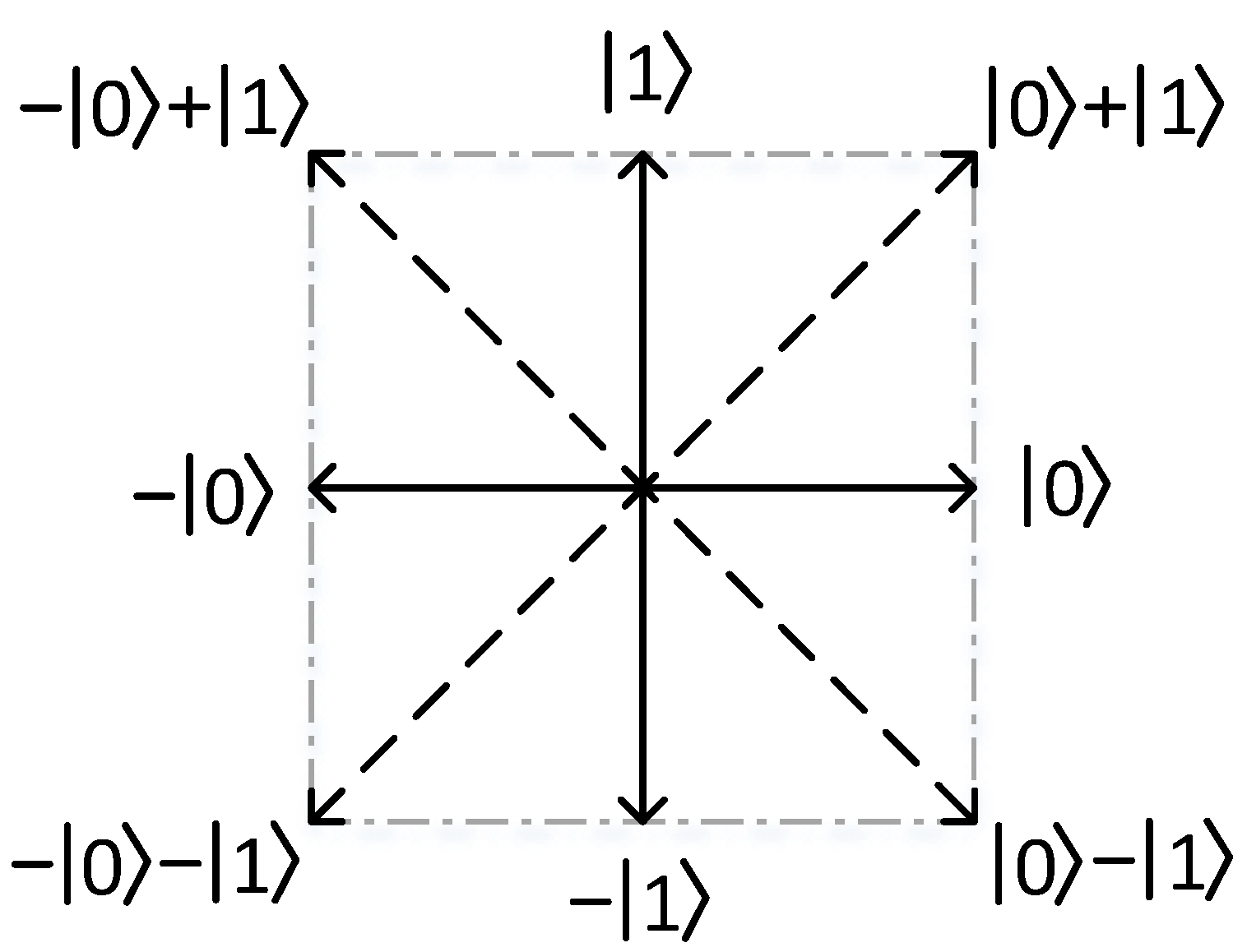
Figure 2. ⁠

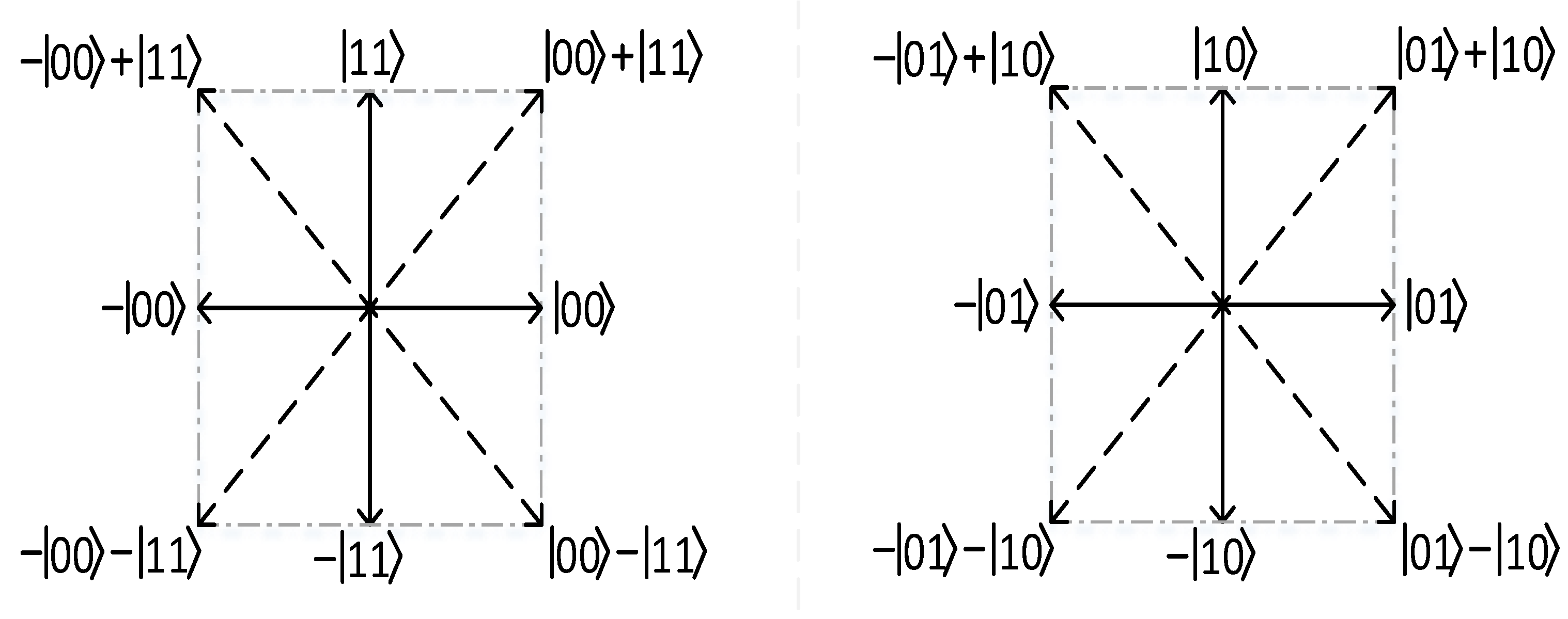
Figure 3. ⁠

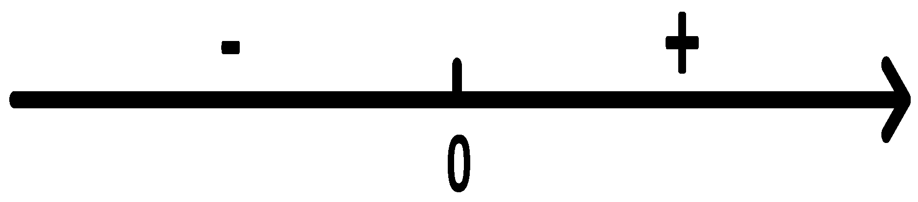
Table 1. ⁠

$\|α〉$	Combinations of the states of two subsystems
$\|Ψ^{+}〉$	1 $(\|u_{1}〉, \|u_{2}〉)$ or $(\|{\bar{u}}_{1}〉, \|{\bar{u}}_{2}〉)$
	2 $(\|u_{1}〉, \|u_{2}〉)$ or $(- \|{\bar{u}}_{1}〉, - \|{\bar{u}}_{2}〉)$
	3 $(- \|u_{1}〉, - \|u_{2}〉)$ or $(- \|{\bar{u}}_{1}〉, - \|{\bar{u}}_{2}〉)$
	4 $(- \|u_{1}〉, - \|u_{2}〉)$ or $(\|{\bar{u}}_{1}〉, \|{\bar{u}}_{2}〉)$
$\|Ψ^{-}〉$	1 $(\|u_{1}〉, \|u_{2}〉)$ or $(- \|{\bar{u}}_{1}〉, \|{\bar{u}}_{2}〉)$
	2 $(\|u_{1}〉, \|u_{2}〉)$ or $(\|{\bar{u}}_{1}〉, - \|{\bar{u}}_{2}〉)$
	3 $(- \|u_{1}〉, - \|u_{2}〉)$ or $(\|{\bar{u}}_{1}〉, - \|{\bar{u}}_{2}〉)$
	4 $(- \|u_{1}〉, - \|u_{2}〉)$ or $(- \|{\bar{u}}_{1}〉, \|{\bar{u}}_{2}〉)$

Table 2. Subsystem states and observation results.

	(b)
$S$	$M_{1}$	$M_{2}$
$(\|a_{1}〉, \|a_{2}〉)$	$\|a_{1}〉 \|b_{1}〉$	$\|a_{2}〉 \|b_{2}〉$
$(\|{\bar{a}}_{1}〉, \|{\bar{a}}_{2}〉)$	$\|a_{1}〉 \|{\bar{b}}_{1}〉$	$\|a_{2}〉 \|{\bar{b}}_{2}〉$
$(\|b_{1}〉, \|b_{2}〉)$	$\|{\bar{a}}_{1}〉 \|b_{1}〉$	$\|{\bar{a}}_{2}〉 \|b_{2}〉$
$(\|{\bar{b}}_{1}〉, \|{\bar{b}}_{2}〉)$	$\|{\bar{a}}_{1}〉 \|{\bar{b}}_{1}〉$	$\|{\bar{a}}_{2}〉 \|{\bar{b}}_{2}〉$
	(b)
$S$	$M_{1}$	$M_{2}$
$(\|a_{1}〉, \|a_{2}〉)$	$\|a_{1}〉 \|b_{1}〉$	$\|a_{2}〉 \|b_{2}〉$
$(\|{\bar{a}}_{1}〉, \|{\bar{a}}_{2}〉)$	$- \|a_{1}〉 \|{\bar{b}}_{1}〉$	$- \|a_{2}〉 \|{\bar{b}}_{2}〉$
$(\|b_{1}〉, \|b_{2}〉)$	$\|{\bar{a}}_{1}〉 \|b_{1}〉$	$\|{\bar{a}}_{2}〉 \|b_{2}〉$
$(- \|{\bar{b}}_{1}〉, - \|{\bar{b}}_{2}〉)$	$- \|{\bar{a}}_{1}〉 \|{\bar{b}}_{1}〉$	$- \|{\bar{a}}_{2}〉 \|{\bar{b}}_{2}〉$
	(c)
$S$	$M_{1}$	$M_{2}$
$(\|a_{1}〉, \|a_{2}〉)$	$\|a_{1}〉 \|b_{1}〉$	$\|a_{2}〉 \|b_{2}〉$
$(- \|{\bar{a}}_{1}〉, - \|{\bar{a}}_{2}〉)$	$\|a_{1}〉 \|{\bar{b}}_{1}〉$	$\|a_{2}〉 \|{\bar{b}}_{2}〉$
$(\|b_{1}〉, \|b_{2}〉)$	$- \|{\bar{a}}_{1}〉 \|b_{1}〉$	$- \|{\bar{a}}_{2}〉 \|b_{2}〉$
$(\|{\bar{b}}_{1}〉, \|{\bar{b}}_{2}〉)$	$- \|{\bar{a}}_{1}〉 \|{\bar{b}}_{1}〉$	$- \|{\bar{a}}_{2}〉 \|{\bar{b}}_{2}〉$
	(d)
$S$	$M_{1}$	$M_{2}$
$(\|a_{1}〉, \|a_{2}〉)$	$\|a_{1}〉 \|b_{1}〉$	$\|a_{2}〉 \|b_{2}〉$
$(- \|{\bar{a}}_{1}〉, - \|{\bar{a}}_{2}〉)$	$- \|a_{1}〉 \|{\bar{b}}_{1}〉$	$- \|a_{2}〉 \|{\bar{b}}_{2}〉$
$(\|b_{1}〉, \|b_{2}〉)$	$- \|{\bar{a}}_{1}〉 \|b_{1}〉$	$- \|{\bar{a}}_{2}〉 \|b_{2}〉$
$(- \|{\bar{b}}_{1}〉, - \|{\bar{b}}_{2}〉)$	$\|{\bar{a}}_{1}〉 \|{\bar{b}}_{1}〉$	$\|{\bar{a}}_{2}〉 \|{\bar{b}}_{2}〉$

Disclaimer/Publisher’s Note: The statements, opinions and data contained in all publications are solely those of the individual author(s) and contributor(s) and not of MDPI and/or the editor(s). MDPI and/or the editor(s) disclaim responsibility for any injury to people or property resulting from any ideas, methods, instructions or products referred to in the content.

© 2025 by the authors. Licensee MDPI, Basel, Switzerland. This article is an open access article distributed under the terms and conditions of the Creative Commons Attribution (CC BY) license (http://creativecommons.org/licenses/by/4.0/).

Copyright: This open access article is published under a Creative Commons CC BY 4.0 license, which permit the free download, distribution, and reuse, provided that the author and preprint are cited in any reuse.

Downloads

Views

154

Comments

Subscription

Notify me about updates to this article or when a peer-reviewed version is published.

MDPI Initiatives

Important Links

Choose an area of interest and we will send you notifications of new preprints at your preferred frequency.

Disclaimer

$\|α〉$	Combinations of the states of two subsystems
$\|Ψ^{+}〉$	1 $(\|u_{1}〉, \|u_{2}〉)$ or $(\|{\bar{u}}_{1}〉, \|{\bar{u}}_{2}〉)$
	2 $(\|u_{1}〉, \|u_{2}〉)$ or $(- \|{\bar{u}}_{1}〉, - \|{\bar{u}}_{2}〉)$
	3 $(- \|u_{1}〉, - \|u_{2}〉)$ or $(- \|{\bar{u}}_{1}〉, - \|{\bar{u}}_{2}〉)$
	4 $(- \|u_{1}〉, - \|u_{2}〉)$ or $(\|{\bar{u}}_{1}〉, \|{\bar{u}}_{2}〉)$
$\|Ψ^{-}〉$	1 $(\|u_{1}〉, \|u_{2}〉)$ or $(- \|{\bar{u}}_{1}〉, \|{\bar{u}}_{2}〉)$
	2 $(\|u_{1}〉, \|u_{2}〉)$ or $(\|{\bar{u}}_{1}〉, - \|{\bar{u}}_{2}〉)$
	3 $(- \|u_{1}〉, - \|u_{2}〉)$ or $(\|{\bar{u}}_{1}〉, - \|{\bar{u}}_{2}〉)$
	4 $(- \|u_{1}〉, - \|u_{2}〉)$ or $(- \|{\bar{u}}_{1}〉, \|{\bar{u}}_{2}〉)$

	(b)
$S$	$M_{1}$	$M_{2}$
$(\|a_{1}〉, \|a_{2}〉)$	$\|a_{1}〉 \|b_{1}〉$	$\|a_{2}〉 \|b_{2}〉$
$(\|{\bar{a}}_{1}〉, \|{\bar{a}}_{2}〉)$	$\|a_{1}〉 \|{\bar{b}}_{1}〉$	$\|a_{2}〉 \|{\bar{b}}_{2}〉$
$(\|b_{1}〉, \|b_{2}〉)$	$\|{\bar{a}}_{1}〉 \|b_{1}〉$	$\|{\bar{a}}_{2}〉 \|b_{2}〉$
$(\|{\bar{b}}_{1}〉, \|{\bar{b}}_{2}〉)$	$\|{\bar{a}}_{1}〉 \|{\bar{b}}_{1}〉$	$\|{\bar{a}}_{2}〉 \|{\bar{b}}_{2}〉$
	(b)
$S$	$M_{1}$	$M_{2}$
$(\|a_{1}〉, \|a_{2}〉)$	$\|a_{1}〉 \|b_{1}〉$	$\|a_{2}〉 \|b_{2}〉$
$(\|{\bar{a}}_{1}〉, \|{\bar{a}}_{2}〉)$	$- \|a_{1}〉 \|{\bar{b}}_{1}〉$	$- \|a_{2}〉 \|{\bar{b}}_{2}〉$
$(\|b_{1}〉, \|b_{2}〉)$	$\|{\bar{a}}_{1}〉 \|b_{1}〉$	$\|{\bar{a}}_{2}〉 \|b_{2}〉$
$(- \|{\bar{b}}_{1}〉, - \|{\bar{b}}_{2}〉)$	$- \|{\bar{a}}_{1}〉 \|{\bar{b}}_{1}〉$	$- \|{\bar{a}}_{2}〉 \|{\bar{b}}_{2}〉$
	(c)
$S$	$M_{1}$	$M_{2}$
$(\|a_{1}〉, \|a_{2}〉)$	$\|a_{1}〉 \|b_{1}〉$	$\|a_{2}〉 \|b_{2}〉$
$(- \|{\bar{a}}_{1}〉, - \|{\bar{a}}_{2}〉)$	$\|a_{1}〉 \|{\bar{b}}_{1}〉$	$\|a_{2}〉 \|{\bar{b}}_{2}〉$
$(\|b_{1}〉, \|b_{2}〉)$	$- \|{\bar{a}}_{1}〉 \|b_{1}〉$	$- \|{\bar{a}}_{2}〉 \|b_{2}〉$
$(\|{\bar{b}}_{1}〉, \|{\bar{b}}_{2}〉)$	$- \|{\bar{a}}_{1}〉 \|{\bar{b}}_{1}〉$	$- \|{\bar{a}}_{2}〉 \|{\bar{b}}_{2}〉$
	(d)
$S$	$M_{1}$	$M_{2}$
$(\|a_{1}〉, \|a_{2}〉)$	$\|a_{1}〉 \|b_{1}〉$	$\|a_{2}〉 \|b_{2}〉$
$(- \|{\bar{a}}_{1}〉, - \|{\bar{a}}_{2}〉)$	$- \|a_{1}〉 \|{\bar{b}}_{1}〉$	$- \|a_{2}〉 \|{\bar{b}}_{2}〉$
$(\|b_{1}〉, \|b_{2}〉)$	$- \|{\bar{a}}_{1}〉 \|b_{1}〉$	$- \|{\bar{a}}_{2}〉 \|b_{2}〉$
$(- \|{\bar{b}}_{1}〉, - \|{\bar{b}}_{2}〉)$	$\|{\bar{a}}_{1}〉 \|{\bar{b}}_{1}〉$	$\|{\bar{a}}_{2}〉 \|{\bar{b}}_{2}〉$

New Algorithm for Entanglement Swapping

Abstract

Keywords:

Subject:

1. Introduction

2. Entanglement Swapping Between Two Bell States

3. The New Algorithm for Entanglement Swapping

4. Discussion

5. Conclusion

Conflicts of Interest

References

MDPI Initiatives

Important Links

Subscribe