Intensity Correlation Imaging and Nonnegative Dynamic Systems

1. Introduction

Recent work of the present Author has succeeded in the vast reduction of integration times that have so long plagued the Hanbury Brown-Twiss effect. The way is now open to reap the advantages of simple, inexpensive flux collecting hardware, immunity to seeing conditions, and unlimited baselines and image resolution. Furthermore since the Brown- Twiss effect has been extended to two-dimensional imaging; it is appropriate that we term the algorithm the Intensity Correlation Imaging (ICI) algorithm.

Within the “The Rise of the Brown-Twiss Effect” surveyed in this special issue the reduction of integration times has been accomplished by means of the Noise Reducing Phase Retrieval (NRPR) algorithm which is embedded within a Stochastic Search algorithm. In the complex analysis of [1], initial conditions, such as small random perturbations in the pixel intensities and other complexities, the algorithm performed very well. However, in this paper we update and simplify the algorithm by constructing a discrete-time dynamic system. Moreover, not only does the algorithm perform as well as the original, but we also introduce the benefits of a nonnegative dynamic systems.

We progress as follows. Section 2 begins with the NRPR algorithm, which contains the correct integration times and sets up the foreground/background dichotomy. Section 3 transforms the NRPR steps into a discrete-time, nonnegative dynamic system. Section 4 merges the dynamic system within the Stochastic search algorithm structured to gradually reduce the “Box” sizes.

2. Description of the NRPR Algorithm

It is supposed that there is an array of flux collecting apertures arranged so as to form a square, evenly spaced grid on the “u-v plane” (which, in interferometry, denotes the Fourier domain projected on the plane perpendicular to the target line-of-sight). The grid has a one-to-one correspondemce to a matrix of $N\times N$ pixels forming the construction of an image of a luminous object amidst a black sky. The defining characteristics of the NRPR algorithm are:

$$\begin{array}{l}g\in {\mathrm{C}}^{N\times N}=\mathrm{Current} \mathrm{value} \mathrm{of} \mathrm{the} \mathrm{estimated} \mathrm{image} \left(\mathrm{pixellated}\right)\\ \overline{g}\in {\mathrm{R}}^{N\times N}=\mathrm{The} \mathrm{true} \mathrm{image}, \mathrm{without} \mathrm{noise}\\ \tau \in {\mathrm{R}}^{N\times N}=\mathrm{Unity} \mathrm{for} \mathrm{for} \mathrm{pixels} \mathrm{constrained} \mathrm{to} \mathrm{have} \mathrm{zero} \mathrm{intensity}\\ \hspace{1em}\hspace{1em}\hspace{1em}\hspace{1em}\hspace{1em} \mathrm{and} \mathrm{zeros} \mathrm{for} \mathrm{pixels} \mathrm{that} \mathrm{are} \mathrm{unconstrained}\\ {\tau }_{\perp }\in {\mathrm{R}}^{N\times N}=I_{N\times N}-\tau ,\mathrm{The} \mathrm{opposite} \mathrm{of} \tau \\ \Im [\dots ]= \mathrm{Two}-\mathrm{dimensional} \mathrm{Fast} \mathrm{Fourier} \mathrm{Transform} \left(\mathrm{unitary}\right)\\ \overline{G}=\Im [\overline{g}]\in {\mathrm{C}}^{N\times N}=\mathrm{The} \mathrm{true} \mathrm{coherence}, \mathrm{without} \mathrm{noise}\\ \mathrm{G} ^\in {\mathrm{R}}^{N\times N}=\mathrm{The} \mathrm{measured} \mathrm{coherence} \mathrm{magnitude} \mathrm{obtained} \mathrm{by} \\ \hspace{1em}\hspace{1em}\hspace{1em}\hspace{1em}\hspace{1em}\hspace{1em} \mathrm{cross}-\mathrm{correlating} \mathrm{the} \mathrm{intensity} \mathrm{signals} \mathrm{from} \mathrm{all} \mathrm{pairs} \\ \hspace{1em}\hspace{1em}\hspace{1em}\hspace{1em}\hspace{1em}\hspace{1em} \mathrm{of} \mathrm{the} \mathrm{flux} \mathrm{collecting} \mathrm{apertures}\\ {\left(\Im [g]\right)}_{kj}=\mathrm{FFT} \mathrm{in} \mathrm{the} \mathrm{u}-\mathrm{v} \mathrm{plane}. {\left(\Im [g]\right)}_{kj}={\left(\Im [g]\right)}_{jk}^{\ast }\\ \mathrm{Re}\left[\dots \right]\triangleq {\displaystyle \frac{1}{2}}\left([\dots ]+{[\dots ]}^{\ast }\right),\hspace{0.33em}\hspace{0.33em}\mathrm{The} \mathrm{real} \mathrm{valued} \mathrm{portion} \mathrm{of} [\dots ]\\ {\mathrm{Re}}_{+}\left[\dots \right]\triangleq \max \left\{0,{\displaystyle \frac{1}{2}}\left([\dots ]+{[\dots ]}^{\ast }\right)\right\},\mathrm{The} \mathrm{real} \mathrm{positive} \mathrm{value} \mathrm{of} [\dots ]\\ \left(A\right)\circ \left(B\right)\triangleq \mathrm{Hadamard} \mathrm{product} \mathrm{of} A \mathrm{and} B\end{array}$$

(1. a-k)

The matrix $\tau$ defines the set of constraints. ${\tau }_{kj}=1$ declares pixel $\left(k,j\right)$ to be constrained to be zero, whereas ${\tau }_{kj}=1$ if $g_{k\hspace{0.17em}j}$is unconstrained. Matrix ${\left({\tau }_{\perp }\right)}_{kj}$ is the opposite; unity for uncnstrained pixels and zero for constrained pixels. The region wherein ${\tau }_{kj}=1$ we have termed “the background”, and the remaining region, “the foreground”. In this scenario, the initial inputs and the subsequent algorithm are defined as in Figure 2.

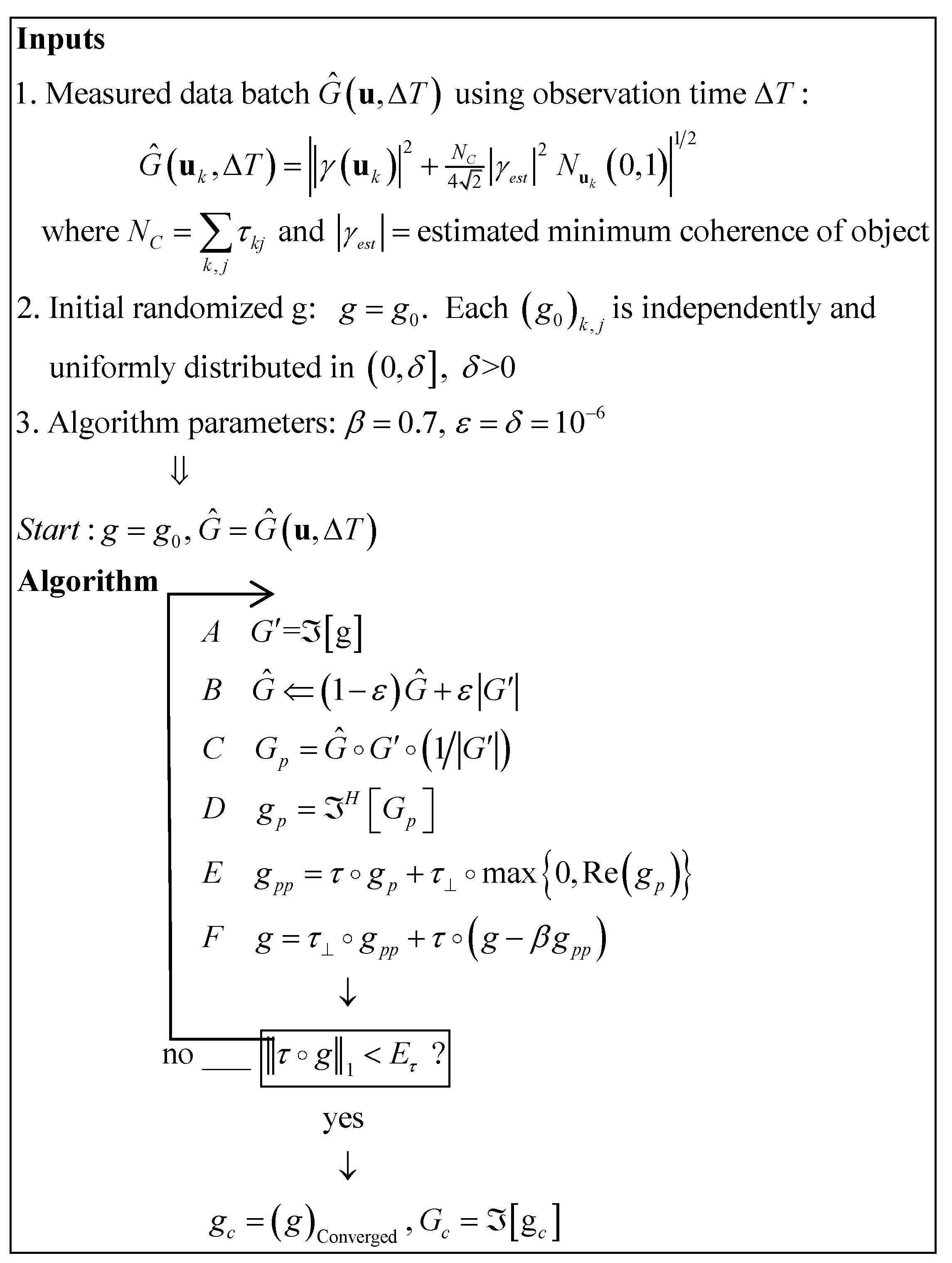
Figure 2 shows the various steps of the NRPR algorithm. There are several initial specifications. The first is the measured coherence magnitude, $\widehat{G}\left(u_k,\Delta T\right)={\left|{\left|\gamma \left(u_k\right)\right|}^2+\frac{N_C}{4\sqrt{2}}{\left|{\gamma }_{est}\right|}^2{N}_{u_k}\left(0,1\right)\right|}^{1/2}$ which obeys a positivity constraint. This is composed of the noise-free normalized coherence magnitude, $\left|\gamma \left(u_k\right)\right|$, where $u_k$ is the relative position vector of a pair of the flux collecting apertures, $N_{u_k}\left(0,1\right)$ is a complex-valued Gaussian noise of zero mean and unit variance and $N_C$ is the number of constrained pixels, i.e. $N_C={\displaystyle \sum _{k=1}^N{\displaystyle \sum _{j=1}^N{\tau }_{kj}}}$ . The formulation of this noise model was accomplished in [2] resulting in an asymptotic expression for the precision estimate of the necessary integration time. The second initial specification is $g=g_0$ where $g_0$ is independently and uniformly distributed in $\left(0,\delta \right]$ where $\delta$ is real and positive. It is these random specifications of the initial values of the pixel intensities that we wish to supplant with a dynamic system having additional simplifications.

It must be emphasized that only a single data batch of measured coherence magnitude measurements will be used in the process by which the zero-noise image is determined. Thus the adaptive algorithms described here do not increase the necessary integration time. However, the adaptive algorithms require repeated NRPR computations, and each such repetition uses a new seed for the randomized initial guess for the image.

The various steps A to F of the algorithm are discussed in References [1,2,3]. The basic computations of NRPR are directed to an hypothesis that a square “box” of size $B_x$ and, positioned in the center of the field of view, contains the noise-free image. Then NRPR is embedded within the Stochastic Search wherein the hypothesis is tested and the noise-free image is discovered.

3. The NRPR Algorithm as a Discrete-Time Dynamic System

As the next step in our analysis, we recast the equations of Figure 2 into a discrete-time dynamic system such that all the principal quantities are indicated by the sequence of integers $k=0,1,\dots \infty$. We start with the initial conditions and the first iteration and recite the sequence of further iterations, keeping the algorithm in its proper order:

$$\begin{array}{c}{\widehat{G}}_{kj}(0)\triangleq {\left|{\left|{\gamma }_{kj}\right|}^2+\frac{N_C}{4\sqrt{2}}{\left|{\gamma }_{est}\right|}^2{N}_{kj}\left(0,1\right)\right|}^{1/2}\\ \mathrm{g}\left(0\right)=\delta \hspace{0.17em}rand\left(N,N\right),\hspace{0.33em}\hspace{0.33em}\delta ={10}^{-6}\\ k=0,1,2,\dots \infty \\ \Downarrow \\ G\left(k+1\right)=\Im \left[\mathrm{g}\left(k\right)\right]\\ \widehat{G}\left(k+1\right)=\left(1-\epsilon \right)\widehat{G}\left(k\right)+\epsilon \left|G\left(k+1\right)\right|\\ \tau \circ g\left(k+1\right)=\tau \circ \left\{g\left(k\right)-\beta \mathrm{Re}\left[{\Im }^H\left(\widehat{G}\left(k+1\right)\circ e^{i\arg \left(G\left(k+1\right)\right)}\right)\right]\right\}\\ {\tau }_{\perp }\circ g\left(k+1\right)={\tau }_{\perp }\circ {\mathrm{Re}}_{+}\left[{\Im }^H\left(\widehat{G}\left(k+1\right)\circ e^{i\arg \left(G\left(k+1\right)\right)}\right)\right]\end{array}$$

(2. a-f)

where the function $rand\left(N,N\right)$ is an $N\times N$ matrix having statistically independent elements that are uniformly distributed in $\left[0,1\right)$. Now consider the equations pertaining to $k=0$ and $1$:

$$\begin{array}{c}{\widehat{G}}_{kj}(0)\triangleq {\left|{\left|{\gamma }_{kj}\right|}^2+\frac{N_C}{4\sqrt{2}}{\left|{\gamma }_{est}\right|}^2{N}_{kj}\left(0,1\right)\right|}^{1/2}\\ \mathrm{g}\left(0\right)=\delta \hspace{0.17em}rand\left(N,N\right),\hspace{0.33em}\hspace{0.33em}\delta \cong {10}^{-6}\\ \Downarrow \\ G\left(1\right)=\Im \left[\delta \hspace{0.17em}rand\left(N,N\right)\right]\\ \widehat{G}\left(1\right)=\left(1-\epsilon \right)\widehat{G}\left(0\right)+\epsilon \delta \left|e^{i\pi \left[2rand\left(N,N\right)-1\right]}\right|=\widehat{G}\left(0\right)+O\left(-\epsilon +\epsilon \delta \right)\\ \tau \circ g\left(1\right)=\tau \circ \left\{g\left(0\right)-\beta \mathrm{Re}\left[{\Im }^H\left(\widehat{G}\left(0\right)\circ e^{i\pi \left[2rand\left(N,N\right)-1\right]}+O\left(-\epsilon +\epsilon \delta \right)\right)\right]\right\}\\ {\tau }_{\perp }\circ g\left(1\right)={\tau }_{\perp }\circ {\mathrm{Re}}_{+}\left[{\Im }^H\left(\widehat{G}\left(0\right)\circ e^{i\pi \left[2rand\left(N,N\right)-1\right]}+O\left(-\epsilon +\epsilon \delta \right)\right)\right]\end{array}$$

(3.a-d)

Ignoring terms of order $\epsilon \mathrm{and} \epsilon \delta$ these relations become:

$$\begin{array}{c}{\widehat{G}}_{kj}\left(1\right)\cong {\widehat{G}}_{kj}\left(0\right)\triangleq {\left|{\left|{\gamma }_{kj}\right|}^2+\frac{N_C}{4\sqrt{2}}{\left|{\gamma }_{est}\right|}^2{N}_{kj}\left(0,1\right)\right|}^{1/2}\\ \tau \circ g\left(1\right)=\tau \circ \mathrm{Re}\left[{\Im }^H\left\{\hspace{0.17em}\left[\delta -\beta \widehat{G}\left(0\right)\right]\circ e^{i\pi \left[2rand\left(N,N\right)-1\right]}\right\}\right]\\ {\tau }_{\perp }\circ g\left(1\right)={\tau }_{\perp }\circ {\mathrm{Re}}_{+}\left[{\Im }^H\left(\widehat{G}\left(0\right)\circ e^{i\pi \left[2rand\left(N,N\right)-1\right]}\right)\right]\\ \Downarrow \mathrm{k}=1,2,\dots ,\infty \\ \widehat{G}\left(k+1\right)=\left(1-\epsilon \right)\widehat{G}\left(k\right)+\epsilon \left|\Im \left[\mathrm{g}\left(k\right)\right]\right|\\ \tau \circ g\left(k+1\right)=\tau \circ \left\{g\left(k\right)-\beta \mathrm{Re}\left[{\Im }^H\left(\widehat{G}\left(k+1\right)\circ e^{i\arg \left(\Im \left[\mathrm{g}\left(k\right)\right]\right)}\right)\right]\right\}\\ {\tau }_{\perp }\circ g\left(k+1\right)={\tau }_{\perp }\circ {\mathrm{Re}}_{+}\left[{\Im }^H\left(\widehat{G}\left(k+1\right)\circ e^{i\arg \left(\Im \left[\mathrm{g}\left(k\right)\right]\right)}\right)\right]\end{array}$$

(4. a-f)

Regarding the second equation above, $\beta \widehat{G}\left(0\right)$ is at least three orders of magnitude larger than $\delta$. Thus:

$\hspace{0.17em}\left[\delta -\beta \widehat{G}\left(0\right)\right]\circ e^{i\pi \left[2rand\left(N,N\right)-1\right]}\cong -\beta \widehat{G}\left(0\right)\circ e^{i\pi \left[2rand\left(N,N\right)-1\right]}$. Then the first three equations above are devoid of the very small quantities $\delta$ and $\epsilon$, therefore we have:

$$\begin{array}{c}{\widehat{G}}_{kj}\left(1\right)\cong {\widehat{G}}_{kj}\left(0\right)\triangleq {\left|{\left|{\gamma }_{kj}\right|}^2+\frac{N_C}{4\sqrt{2}}{\left|{\gamma }_{est}\right|}^2{N}_{kj}\left(0,1\right)\right|}^{1/2}\\ \tau \circ g\left(1\right)=-\beta \tau \circ \mathrm{Re}\left[{\Im }^H\left(\widehat{G}\left(0\right)\circ e^{i\pi \left[2rand\left(N,N\right)-1\right]}\right)\right]\\ {\tau }_{\perp }\circ g\left(1\right)={\tau }_{\perp }\circ {\mathrm{Re}}_{+}\left[{\Im }^H\left(\widehat{G}\left(0\right)\circ e^{i\pi \left[2rand\left(N,N\right)-1\right]}\right)\right]\\ \Downarrow \mathrm{k}=1,\dots ,\infty \\ \widehat{G}\left(k+1\right)=\left(1-\epsilon \right)\widehat{G}\left(k\right)+\epsilon \left|\Im \left[\mathrm{g}\left(k\right)\right]\right|\\ \tau \circ g\left(k+1\right)=\tau \circ \left\{g\left(k\right)-\beta \mathrm{Re}\left[{\Im }^H\left(\widehat{G}\left(k+1\right)\circ e^{i\arg \left(\Im \left[\mathrm{g}\left(k\right)\right]\right)}\right)\right]\right\}\\ {\tau }_{\perp }\circ g\left(k+1\right)={\tau }_{\perp }\circ {\mathrm{Re}}_{+}\left[{\Im }^H\left(\widehat{G}\left(k+1\right)\circ e^{i\arg \left(\Im \left[\mathrm{g}\left(k\right)\right]\right)}\right)\right]\end{array}$$

(5. a-f)

This dynamic system replaces six steps per iteration with three steps. Note that the quantity $e^{i\pi \left[2rand\left(N,N\right)-1\right]}$ is the phase factor of the Fourier transform of the random initial pixel intensities. The new initial conditions in Equations (5. b-c) are correct to within $\epsilon$ and $\delta$ (${10}^{-6}$). This means that to the same small error the complete history of the dynamic system is essentially identical to that of the original NRPR in Figure 2. In particular one must note that (5.b) also leads to the convergence of $\tau \circ g\left(k\right)$ to zero as demonstrated in Reference [1] . Therefore in the limit, ${\tau }_{\perp }\circ g\left(k\right)$ is the ultimate nonnegative dynamic system.

Clearly the phase factor, $e^{i\pi \left[2rand\left(N,N\right)-1\right]}$, in $\tau \circ g\left(0\right) \mathrm{and} {\tau }_{\perp }\circ g\left(0\right)$ is a statistical ensemble that encompasses all possible coherence phases. Thus there is a very significant non-zero probability that on any one trial NRPR converges to of the correct coherence phase and magnitude and therefore to the noise-free image.

4. The Stochastic Search Algorithm for Sequential Box Sizes

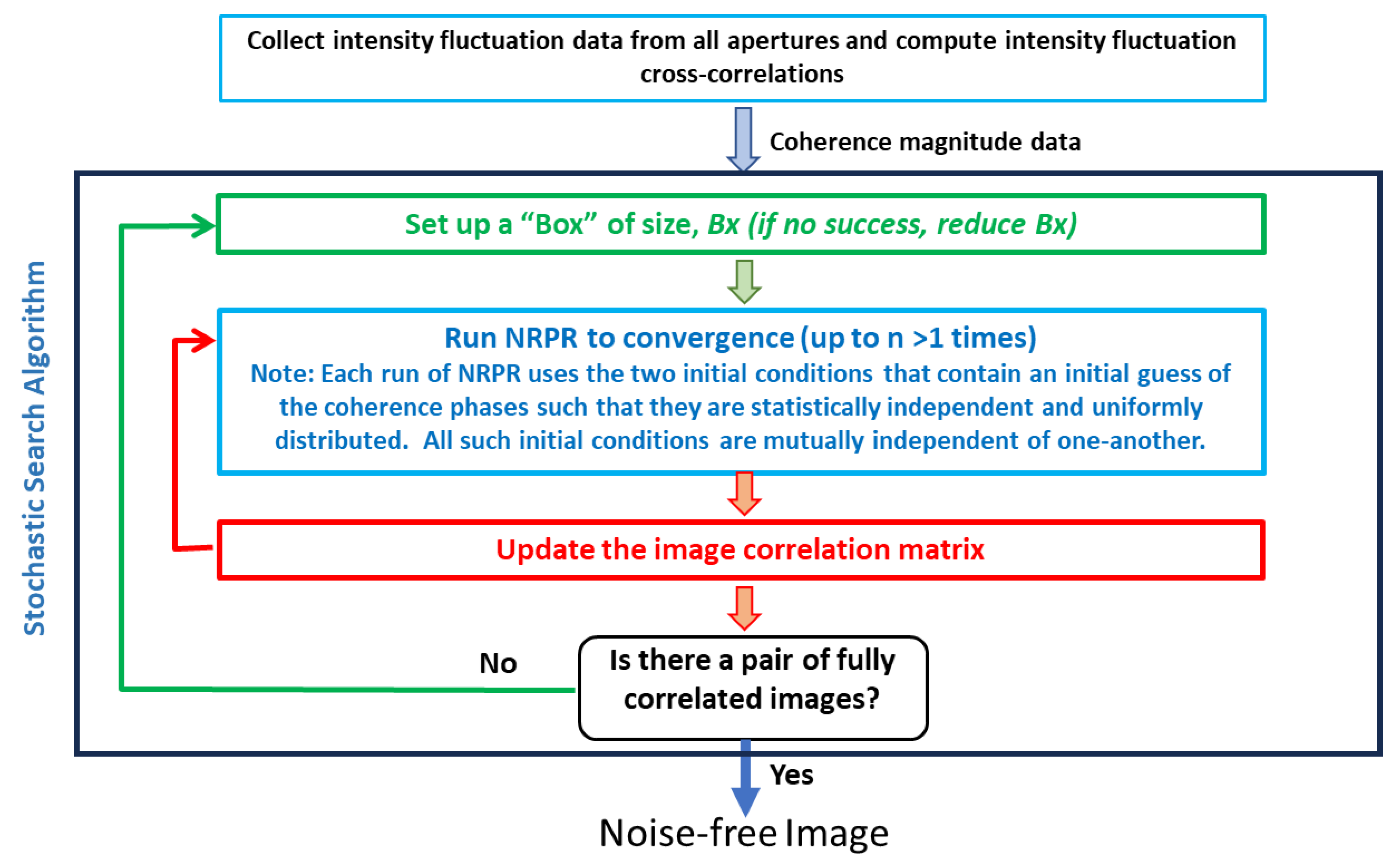
In this Section we consider the Stochastic Search algorithm employing random coherence phases within the two initial conditions rather than random pixel intensities. Figure 3 shows that the embedded NRPR runs (in blue) use statistically independent and uniformly distributed coherence phases spanning $\left[-\pi ,\pi \right)$. The search sets up a square “Bx” and runs NRR $n>1$ times until there are two images that are fully correlated. In that case, the two outcomes are the noise-free image (baring 180 degrees of rotation or translations). If there are no such correlations within n computations, then the algorithm reduces the box size and tries again. If by chance a converged image has pixel intensities that reside outside of the box, this indicates that the box is too small to contain the illuminated object, and the box size must be enlarged. Overall this is the process by which the Stochastic Search validates the hypotheses of the box size.

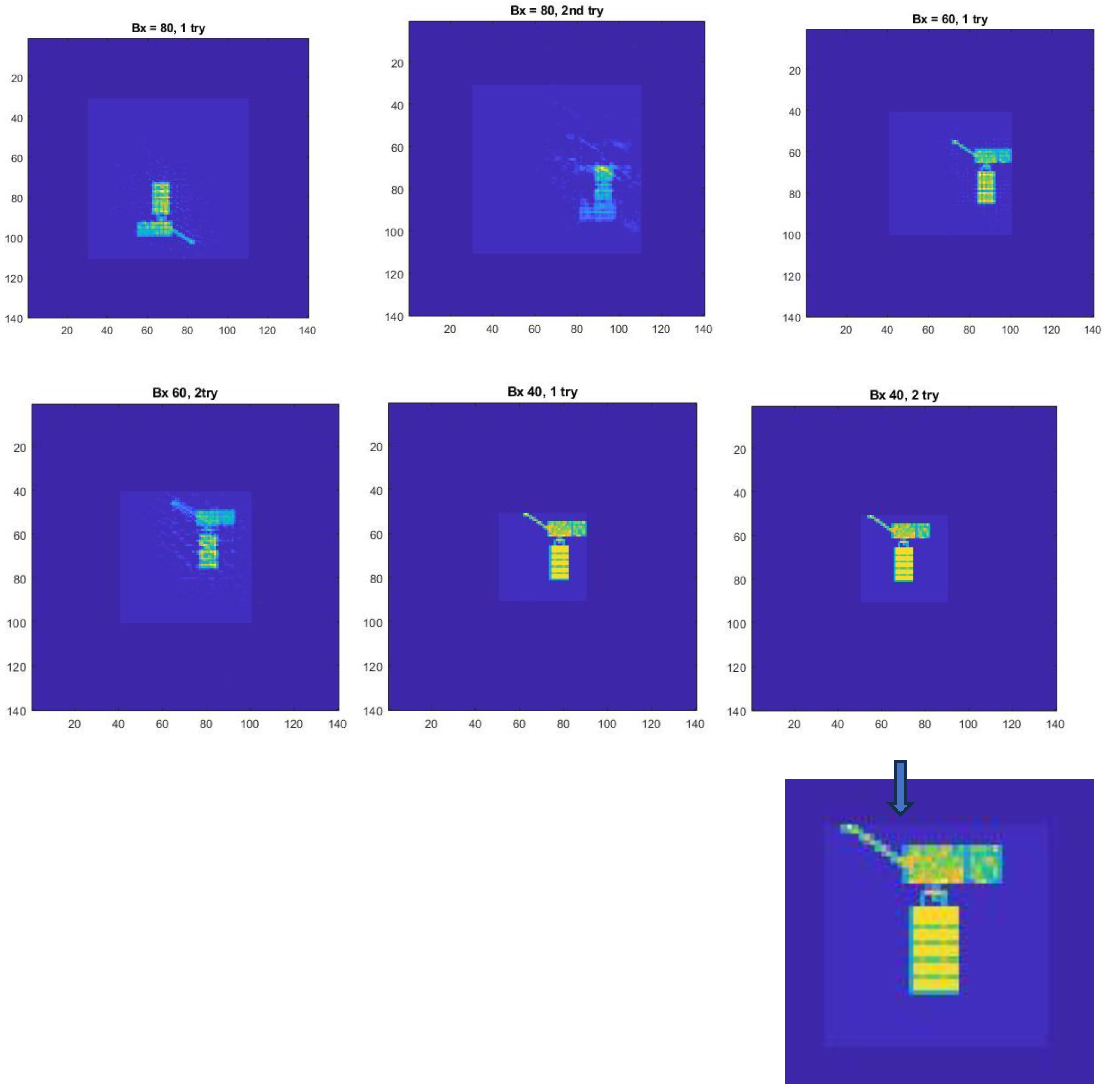
In Figure 4 we demonstrate that the dynamic system (5. a-f) behaves essentially as in References [1,2,3] when in the case that the smallest box size does fully contain the illuminated object. Alternately, one can start with a box size that is smaller than the illuminated object and then increase the box sizes until the noise-free image is found. With this strategy, the number of NRPR computations is distinctly reduced. In fact, if the number of runs is large for the case of decreasing box size, then for the same image, the number of runs for the case of increasing box sizes is halved. The latter strategy, as mentioned in Reference[1] is clearly superior.

5. Conclusions

Reference [1] created an algorithm that emphatically reduced the integration times of the Brown-Twiss effect as applied to two-dimensional imaging (termed ICI). However, there were a number of complexities in the algorithm that merited simplification. This paper has succeeded in streamlining the ICI algorithm by transforming the six steps of the original algorithm into a discrete-time, nonnegative dynamic system having a three dimensional state space. It is demonstrated that this dynamic system fully replicates the original to within $O\left(\epsilon \right)$. Furthermore, the simplified product, being a nonnegative system [4], is well suited to partner with Artificial Intelligence automation such as nonnegative spiking neural networks. Such automation can be expected in the near future.

The Author is an Independent Researcher.

References

- Hyland, D.C. Analysis and Refinement of Intensity Correlation Imaging. Applied Optics 2023, 62, 5683–5695. [Google Scholar] [CrossRef] [PubMed]
- Hyland, D.C. Improved Integration Time Estimates for Intensity Correlation Imaging. Applied Optics 2022, 61, 10002–10011. [Google Scholar] [CrossRef] [PubMed]
- Hyland, D.C. Algorithm for Determination of Image Domain Constraints for Intensity Correlation Imaging. Applied Optics 2022, 61, 10425–10432. [Google Scholar] [CrossRef] [PubMed]
- Haddad, W.; Chellaboina, V.; Hui, Q. Nonnegative and Compartmental Dynamical Systems; Copyright C; Princeton University Press, 2010. [Google Scholar]