Preprint
Article

This version is not peer-reviewed.

Local-Equilibrium Approximation in Non-Equilibrium Thermodynamics of Diffusion

A peer-reviewed article of this preprint also exists.

Submitted:

12 February 2025

Posted:

14 February 2025

You are already at the latest version

Abstract

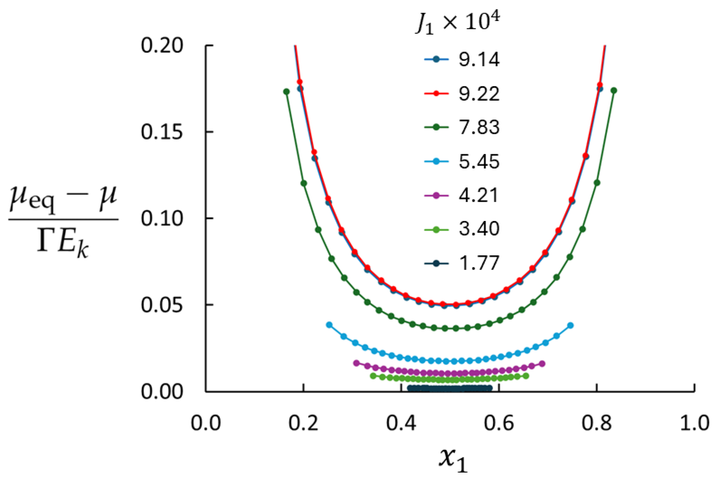
The local equilibrium approximation (LEA) is a central assumption in many applications of non-equilibrium thermodynamics involving the transport of energy, mass, and momentum. However, assessing the validity of the LEA remains challenging due to the limited development of tools for characterizing non-equilibrium states compared to equilibrium states. To address this, we have developed a theory based on kinetic theory, which provides a nonlinear extension of the telegrapher’s equation commonly discussed in non-equilibrium frameworks that extend beyond the LEA. A key result of this theory is a steady-state diffusion equation that accounts for the constraint imposed by available thermal energy on the diffusion flux. The theory is suitable for analysis of steady-state composition profiles and can be used to quantify the deviation from local equilibrium. To validate the theory, we performed molecular dynamics simulations. The results show that deviation from local equilibrium can be systematically quantified, and for the diffusion process we have studied here, we have confirmed that the LEA remains accurate even under extreme concentration gradients in gas mixtures.

Keywords: 
;  ;  ;  ;  ;  

1. Introduction

The concept of local equilibrium in non-equilibrium thermodynamics comes up in analyses of transport processes such as heat- and mass transport. In so-called linear non-equilibrium thermodynamics, one assumes local equilibrium, meaning that the local version of the Gibbs-Duhem equation is assumed valid. The assumption is closely related to assuming that the local non-equilibrium entropy can be approximated by its equilibrium value in the entropy balance, which is the basis for finding the entropy production and coupled flux-force relations [1]. Whereas entropy is well understood and modeled for thermodynamic systems at equilibrium, the situation for systems out of equilibrium is less clear [2]. Usually, the assumption is introduced as an approximation and justified with successful consistency tests as "circumstantial evidence". This is not satisfactory, and the extremely large forces and fluxes used in computer simulations that are necessary for acceptable signal to noise ratios in the results, raise a need for a quantitative examination of the local-equilibrium approximation (LEA) [3].
An alternative approach is to assume the opposite, viz. local non-equilibrium, derive the corresponding theory whenever possible, and determine the deviation from local equilibrium. A powerful criterion for this deviation is the difference in equilibrium and non-equilibrium entropy. Several theories for the non-equilibrium entropy have been proposed for heat transport and diffusion, see e.g. [4,5], and references therein. Cimmelli et al. [4] have given a very thorough discussion of four different theories and compared their pros and cons. They discuss the theories’ relation to kinetic theory, valid for low-density gases and conclude that in general, continuum theories that are compatible with kinetic theory are less universal (e.g. limited to large Knudsen numbers, monatomic gas), but more predictable than other theories.
In the present work, we pursue developing a theory for transport processes that do not depend on the LEA. The theory is based on the Boltzmann equation and developed for diffusion in a binary gas mixture. It is then used to analyze results from molecular dynamics simulations of binary diffusion in a Lennard-Jones/spline (LJs) system. The two components are identical (a "color experiment"), which simplifies the analysis and enables comparison with self-diffusion data. This is one of the simplest cases one can imagine for a study of a transport process. Our intention is to force the diffusion process as much as the system allows in an attempt to provoke a deviation from local equilibrium. The results are compared with what we get from Fick’s law and with data from equilibrium simulations (mean square displacement).

2. Theory

2.1. Fick’s Law

In most common applications, diffusion is usually expressed in the form of Fick’s law, which states that the diffusion flux J i of component i is proportional to the gradient in the concentration n i of the corresponding component in the mixture
J i = D n i
where D is the diffusion coefficient1. Fick’s law for gas mixtures can be obtained ab initio from kinetic theory in the short mean free path limit, meaning that it holds for descriptions on length scales much longer than the mean free path. The divergence of Eq. (1) at constant temperature and mass density, combined with the mass conservation law
t n i + · J i = 0
yields the well-known diffusion equation, under the additional approximation that D is independent of n i ,
t n i = D 2 n i .
Fick’s law can also be obtained using the non-equilibrium thermodynamics methodology. Considering a binary mixture at isothermal conditions, the entropy differential is
d s = μ 1 T d x 1 μ 2 T d x 2 = μ T d x 1
where s is the entropy per particle, T the temperature, and μ i and x i are the chemical potential and mole fraction of component i, respectively. We have used that d x 1 = d x 2 and introduced μ = μ 1 μ 2 . In order to keep the analysis relatively simple, we will in the following neglect the Dufour effect in the special case we consider here, in other words neglect the heat flux accompanying diffusion. Using the mass conservation law, we obtain the entropy balance
n t s = μ T · J 1 = · μ J 1 T J 1 · μ T = · J s + σ
where we have identified the entropy flux J s = μ J 1 / T and the entropy production rate σ = J 1 · μ / T . The latter is expressed on the standard form as a product of the flux J 1 and its conjugate driving force μ / T . Assuming that this driving force is proportional to J 1 by some proportionality factor r > 0 guarantees the positivity of the entropy production rate, and gives the following relation at isothermal conditions:
r J 1 = μ T J 1 = 1 r T μ n 1 n 1 = D n 1 r = μ / n 1 T D .
Thus, we arrive at Fick’s law by the general requirement that the flux is a linear combination of the thermodynamic driving forces in the system, where in this case μ / T is the sole driving force. The identification of D from r clarifies the connection.

2.2. Generalized Diffusion Equation
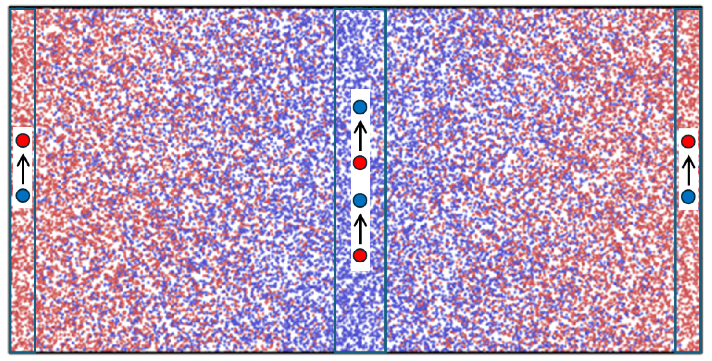
While Fick’s law is adequate for describing diffusion processes when the system is everywhere in local equilibrium, significant departures from local equilibrium expose its unphysical features. For example, according to Fick’s law, a local change in the composition or flux anywhere in the system will immediately affect the evolution of the physical state everywhere else in the system. That is, Fick’s law propagates information across the spatial domain at an unphysical infinite speed, when it can easily be argued that this propagation rate must have a speed limit dictated by the molecular velocities involved (the "causality problem" [6]). We seek a more general evolution equation of diffusion from the Boltzmann equation, which is not constrained by assumptions of local equilibrium. Following the work of Snell, Aranow and Spangler, the general equation of motion for component i in an isothermal multicomponent mixture, as obtained from the Boltzmann equation, is [7]
t ρ i u i = · A i B i ρ i u i u + u u i u u + x i k ξ i k x k u k u i n i μ i
where ρ i and u i are the mass density and the mean velocity of component i, respectively, u is the local barycentric velocity of the mixture, and ξ i k is a friction coefficient describing the exchange of momentum between components i and k. The tensor A i denotes viscous contributions,
A i = x i k ζ i k 2 3 η i k I · x k u k + η i k x k u k + x k u k T ,
where ζ i k and η i k are coefficients related to the bulk and shear viscosity, respectively. We refer the interested reader to [7] for their definitions. We do not go into those here, as they are not of consequence for the analysis in this work. The tensor B i represents the traceless part of the diffusion momentum outer product (indicated by the symbol ¯ ):
B i = ρ i u i u u i u ¯ = ρ i u i u u i u 1 3 I Tr u i u u i u .
Consider a mixture with no barycentric flow, u = 0 . The equation of motion simplifies somewhat:
t ρ i u i + · ρ i u i u i ¯ = x i k ξ i k x k u k u i n i μ i + · A i .
We identify the fluxes J i = n i u i u = n i u i and consider a binary mixture. The difference between the equations of motion for the two components is
t m 1 J 1 m 2 J 2 + · m 1 J 1 J 1 ¯ n 1 m 2 J 2 J 2 ¯ n 2 = 2 x 1 x 2 ξ J 2 n 2 J 1 n 1 n 1 μ 1 + n 2 μ 2 + · A 1 A 2 .
where m i is the molecular mass of component i and the friction coefficients are symmetric, ξ i k = ξ k i = ξ . We now use that J 2 = J 1 and use μ i = μ i + Γ k B T ln x i where Γ is the thermodynamic factor. Eq. (11) can then be reduced to
m ¯ t J 1 + m ¯ n · J 1 J 1 ¯ c 1 x 1 1 c 1 1 x 1 1 2 · A 1 A 2 = ξ J 1 n Γ n k B T x 1
where m ¯ = ( m 1 + m 2 ) / 2 is the average molecular mass, and c 1 = m 1 / ( m 1 + m 2 ) . In the system we consider here, m 1 = m 2 = m , so that c = 1 / 2 , which is used in the following. We see that under conditions where the terms on the left-hand side of Eq. (12) are small, that is when temporal and spatial variations in the flux are small, we reproduce Fick’s law. This allows us to identify the friction coefficient ξ in terms of the diffusion coefficient:
J 1 = Γ n 2 k B T ξ x 1 = n D x 1 ξ = Γ n k B T D .
Using the product rule, we can split the term involving the divergence of the traceless kinetic energy tensor:
· J 1 J 1 ¯ 1 x 1 1 1 x 1 = 1 x 1 1 1 x 1 · J 1 J 1 ¯ 1 x 1 2 + 1 ( 1 x 1 ) 2 J 1 J 1 ¯ · x 1 .
Furthermore, when the two components are physically identical, the viscosity coefficients ζ i j and η i j in Eq. (8) are equal for both components, so that all contributions to A i are proportional to u , which vanishes in the absence of barycentric motion. Thus, A i = 0 in this case. Inserting Eq. (14) into Eq. (12) and removing viscous terms, we find
τ t J 1 + 1 2 n 1 x 1 1 1 x 1 · J 1 J 1 ¯ + J 1 = D 1 m 2 Γ n 2 k B T 1 x 1 2 + 1 ( 1 x 1 ) 2 J 1 J 1 ¯ · n 1
where we identified the characteristic time τ = m n / ξ = m D / ( Γ k B T ) . We note that when the terms involving the divergence of the traceless kinetic energy tensor can be neglected, this reduces to
τ t J 1 + J 1 = D n 1 ,
the divergence of which leads to the well-known telegrapher’s equation for n 1 , which is a damped wave equation describing waves propagating with a characteristic speed D / τ and attenuated over a characteristic time τ . Eq. (1) corresponds to Eq. (16) in the limit τ 0 , which corresponds to a diverging wave speed that leads to the unphysically instantaneous propagation of information across the domain. The telegrapher’s equation takes into account the inertia of molecular motion that resists rapid changes to the diffusion flux, and its connection to non-equilibrium thermodynamics is thoroughly discussed in the work by Jou, Casas-Vázquez and Lebon [8]. There, the authors arrive at equations of the telegrapher type by means of the thirteen moment approximation, which is on the same order as Eq. (15) with respect to spatial and temporal correlations. We can thus expect that the relationship between τ and D at this level of approximation should be corrected for higher order fluxes in order to match real data, justifying an a priori unknown correction factor α such that the true relaxation time is α τ .
For sake of simplicity, we will in the following restrict our attention to self-diffusion along a single dimension in three-dimensional space. The case of two identical components (self-diffusion) is particularly simple because the viscous terms vanish. Introducing also the correction factor α , Eq, (15) is replaced by the one-dimensional equation
α τ t J 1 + 1 3 n 1 x 1 1 1 x 1 J 1 2 + J 1 = D 1 α m J 1 2 3 Γ n 2 k B T 1 x 1 2 + 1 ( 1 x 1 ) 2 n 1 .
Rearranging Eq. (17) and using that r J 1 represents a generalized driving force (see Eq. (6)), we find
r J 1 = 1 α m J 1 2 3 Γ n 2 k B T 1 x 1 2 + 1 ( 1 x 1 ) 2 μ 1 , eq T α m n x 1 T t J 1 + 1 3 n 1 x 1 1 1 x 1 J 1 2 .
In Eq. (18), we have specified that the chemical potential μ 1 , eq is the equilibrium value, i.e. that obtained from the equation of state to distinguish it from the non-equilibrium value to be introduced below. We can now identify the right-hand side of Eq. (18) as a generalized driving force. The expected entropy production rate is therefore
σ = i { J i 1 α m J i 2 3 Γ n 2 k B T 1 x i 2 + 1 ( 1 x i ) 2 μ i , eq T + J i α m n x i T t J i + 1 3 n 1 x i 1 1 x i J i 2 } .
In order to connect the departure from Fickian diffusion to the deviation from local equilibrium, we consider a generalized entropy s, which reduces to the local equilibrium entropy s eq when the system relaxes to local equilibrium. Taking the mole fractions and fluxes as independent variables, the differential is
d s = μ 1 T d x 1 μ 2 T d x 2 + B 1 d J 1 + B 2 d J 2
where μ i is now a generalized chemical potential of component i. In order to have correspondence to the equilibrium entropy, we must have that lim J i 0 μ i = μ i , eq . We can determine B i by assuming that the equation of motion arises from a generalized driving force that is proportional to J i , again ensuring the positivity of the resulting entropy production rate. We note that the contribution from the time derivative of J i to σ is
σ i α m J i n x i T t J i ,
which allows us to deduce that
n t s α m J i n x i T t J i d s α m J i n 2 x i T d J i B i = α m J i n 2 x i T .
Now, we use that x 1 + x 2 = 1 to simplify Eq. (20) to
d s = μ T d x 1 + B 1 d J 1 + B 2 d J 2
where μ = μ 1 μ 2 , equivalent to the definition in Eq. (4). We can then obtain the J i -dependence of μ through symmetry of mixed derivatives
μ / T J i = 2 s J i x 1 = 2 s x 1 J i = B i x 1 = α n 2 T x 1 m J i x i = α m J 1 n 2 x 1 2 T i = 1 α m J 2 n 2 x 2 2 T i = 2
Combined with the correspondence requirement to s eq and that J 1 + J 2 = 0 we find
μ T = μ eq T + 0 J 1 d J α m J n 2 T 1 x 1 2 + 1 ( 1 x 1 ) 2 = μ eq T + α m J 1 2 2 n 2 T 1 x 1 2 + 1 ( 1 x 1 ) 2
We identify the second term on the right-hand side as the kinetic energy associated with species interdiffusion, multiplied by a factor α / T . This implies that in the non-equilibrium situation, the equilibrium chemical potential is replaced by a generalized chemical potential where a term proportional to the kinetic energy of diffusion is subtracted. This agrees with the assessment by de Groot and Mazur, who arrived at a similar generalized driving force by considering the necessity of subtracting the kinetic energy of diffusion from the typically defined internal energy to obtain the truly internal energy [9]. We may quantify the departure from local equilibrium using the deviation of the local chemical potential from its equilibrium value:
μ eq μ = α m J 1 2 2 n 2 1 x 1 2 + 1 ( 1 x 1 ) 2 = α m u 1 2 2 + m u 2 2 2 ,
which reproduces the de Groot and Mazur result in the special case α = 1 . We restrict our attention to the steady-state equation of motion, where t J 1 = 0 and J 1 t x 1 = 0 . This now reads
J 1 = D 1 μ eq μ Γ E k n 1
where E k = 3 k B T / 2 is the average molecular translational kinetic energy. Fick’s law with constant D predicts a constant composition gradient in steady state, according to Eq. (3). According to Eq. (27), we expect to see a curved composition profile when the local deviation in chemical potential from the local equilibrium value is significant relative to Γ E k . The mechanism at play here is that of the diffusion process approaching its speed limit dictated by the local distribution of molecular velocities. Whereas a Fickian model would violate this speed limit by allowing the diffusion flux to increase beyond the rate of transport permissible by the ballistic motion of molecules at a given temperature, this generalized formulation properly enforces said speed limit in a continuous and physically consistent manner. Investigating the curvature of the steady-state composition profile resulting from a large imposed diffusion flux allows us to properly quantify the deviation from local equilibrium.
We note that for fixed x i , we can use the result for B i , Eq. (22), in Eq. (20) and integrate to give
s s eq = i α m J i 2 2 n 2 x i T = α m J 1 2 2 n 2 T 1 x 1 + 1 1 x 1 = α m J 1 2 2 n 2 x 1 1 x 1 T ,
which shows that the non-equilibrium entropy s is always smaller than the equilibrium value, which is consistent with the second law. The absolute deviation in the entropy from the local equilibrium value has a minimum at x 1 = 0.5 .

3. MD Simulations

Non-equilibrium molecular dynamics (NEMD) simulations were carried out to provide data for use with the theory. The layout of the MD system is shown in Figure 1. The system consisted of N = 32 , 768 Lennard-Jones/spline (LJs) particles [10] in a rectangular cuboid with aspect ratio L x : L y : L z = 2 : 1 : 1 . The LJs potential is a smoothly truncated Lennard-Jones potential with cut-off distance r c 1.7 σ . The MD box had periodic boundary conditions in all three directions. The box was divided into 64 layers of equal thickness in x-direction for recording local data of temperature, density, composition, etc.. The particles were of two types, 1 ("red") and 2 ("blue") with exactly the same mass and potential parameters.
Concentration gradients and diffusive mass fluxes were generated with an in-house NEMD code using the MEX algorithm [3]. The MEX algorithm works so that a randomly picked particle of type 2 is changed to type 1 in one of the control volumes at the box ends (see Figure 1) while a particle of type 1 is changed to type 2 in the central volume at the same time. The overall concentration was thus kept constant. The identity swapping occurred at regular intervals. By changing the swapping frequency, the diffusion flux was controlled from zero (equilibrium) to maximum (saturated control volumes, i.e.  x 1 = 1 at the box ends and x 1 = 0 in the box center). If there was no candidate particles to swap in either control volume, the swapping was skipped.
The simulations started from a FCC lattice configuration with N 1 = N 2 = N / 2 . To prevent heating of the system due to the entropy production, the system temperature was controlled by thermostating each of the 64 layers to the same set temperature and the overall density was controlled by the total number of particles in the fixed box volume. Six cases were generated with the density and temperature as listed in Table 1. All values of physical properties reported here are in Lennard-Jones units. The mean free path, λ , was estimated from elementary kinetic theory as λ = 1 / ( π 2 n ) and compared with half box length, L x / 2 . Case 1 is a very dilute (ideal) gas which is not well suited for MD simulations due to the fact that the particles are mostly in free flight, the mean free path is of the same order as L x / 2 (the distance between the swapping layers) in this case. Nevertheless, this low-density case was included here because of the kinetic-theory basis for the analysis. Case 6 is close to the LJs system’s dew point (at n = 0.026 for T = 0.7 ). When the mean free path is much larger than the range of the potential, particles may overlap at the end of a time step. To avoid strong accelerations if this happens, the particles were given a reflecting "shield" at r i k = 0.8 .
A total of 4,000,000 time steps of length δ t = 0.002 in Lennard-Jones units were used to produce data for analysis. The final 2,000,000 time steps were used to represent steady-state with J = 0 .

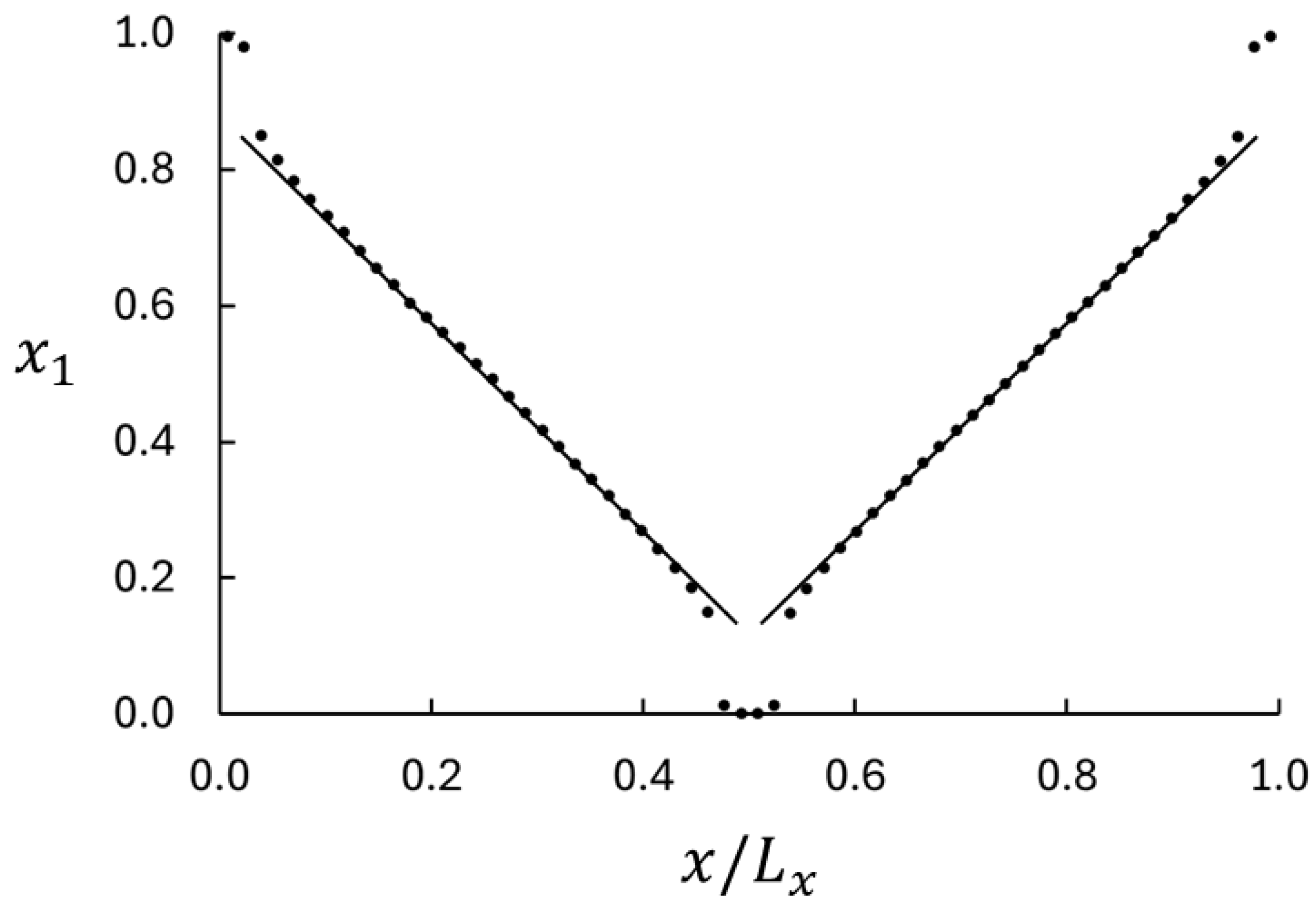
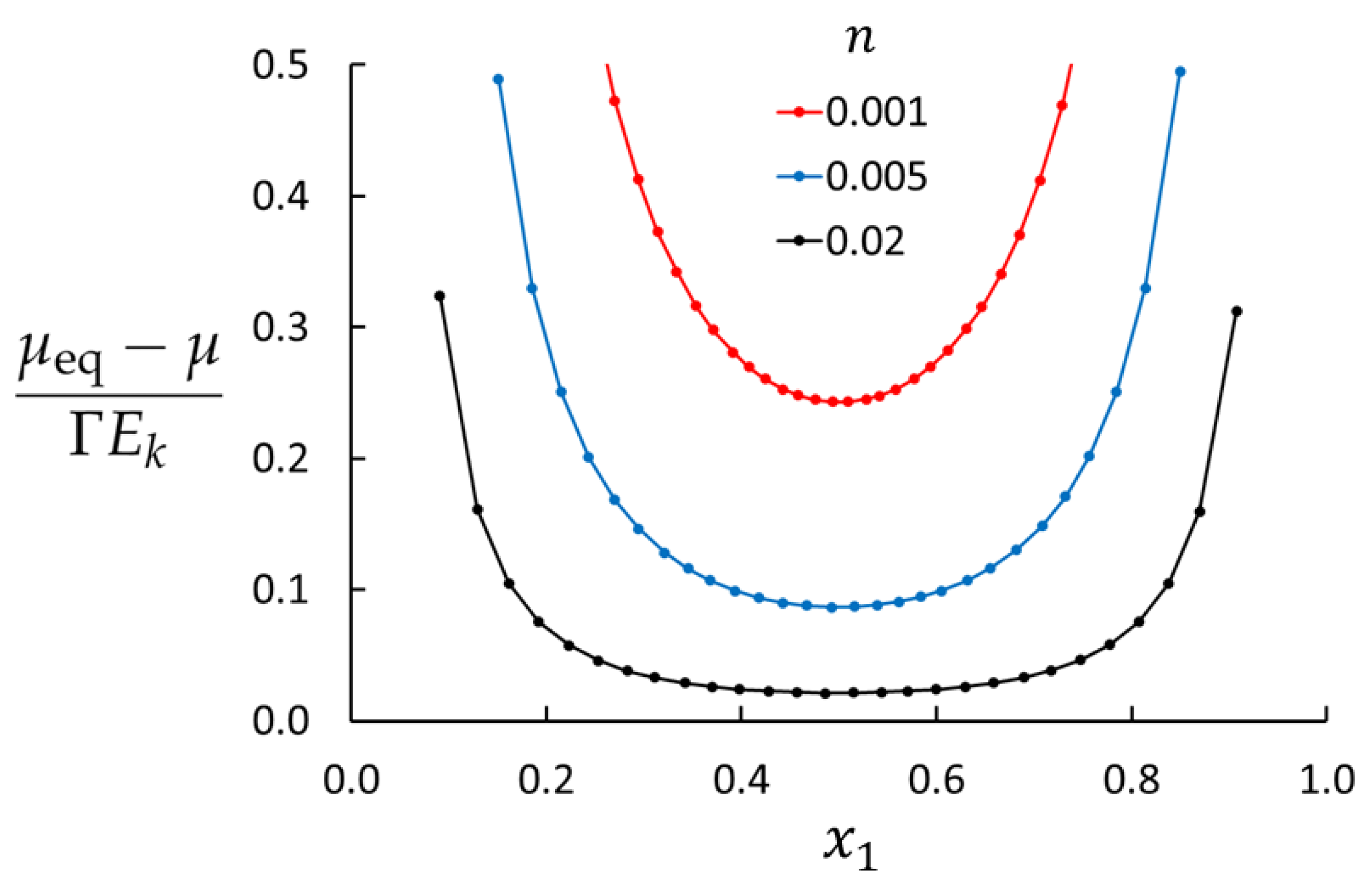
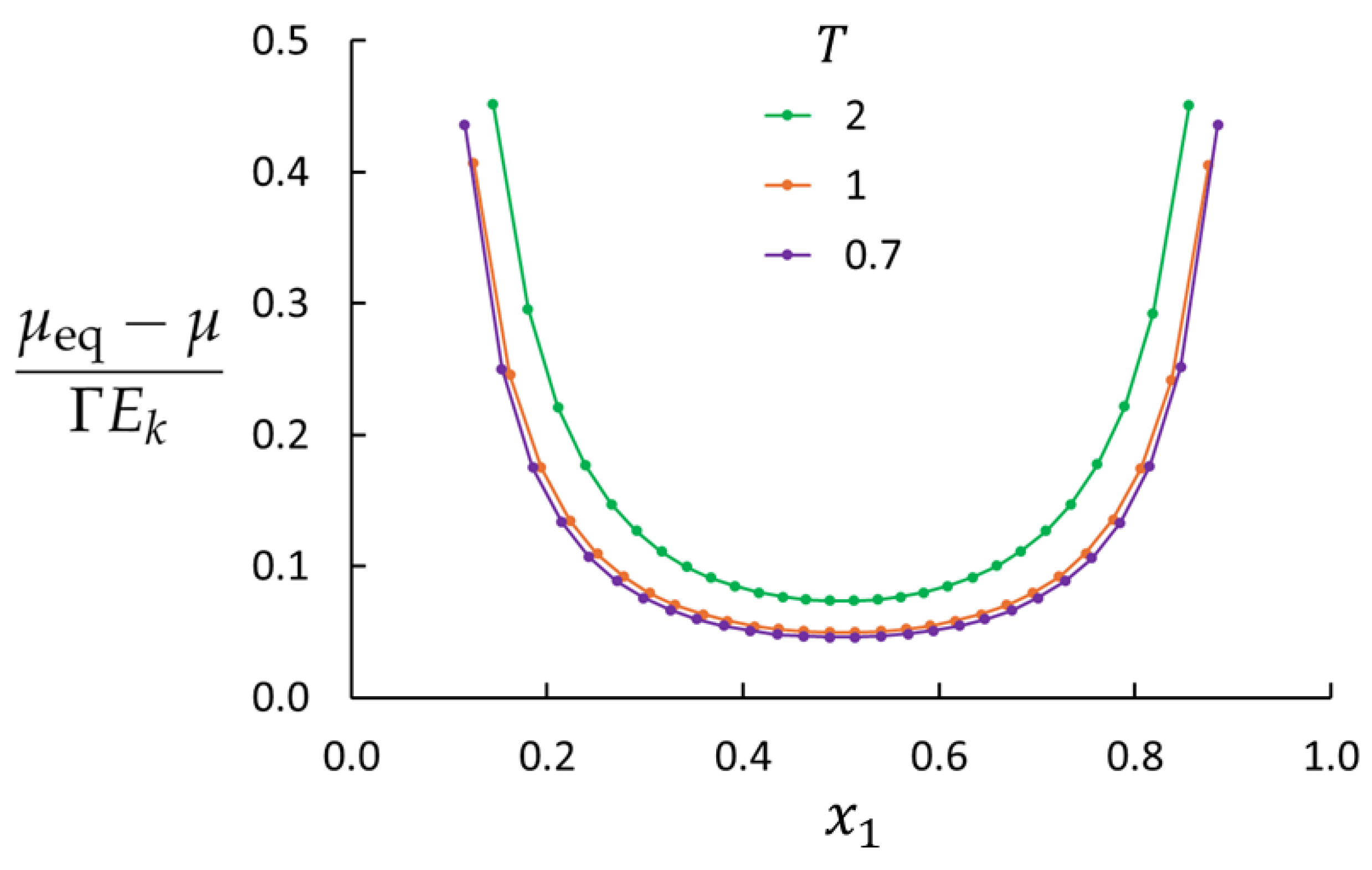
4. Results and Discussion

According to Darken’s second equation [11], the mutual diffusion coefficient D in a binary mixture relates to the self-diffusion coefficients D 1 and D 2 , as
D = ( x 1 D 1 + x 2 D 2 ) Γ .
In our ideal case, Γ = 1 and D 1 = D 2 , so that the diffusion coefficient we compute by generating a diffusive flux in the two-component system is simply the self-diffusion coefficient. This enables a comparison between the binary diffusion coefficient, generated with extreme fluxes and forces, and self-diffusion coefficients generated at global equilibrium.
We shall now analyze the binary diffusion data using the theory developed in Section 2.2. Central in this analysis is the curvature of the mole-fraction profile and the deviation from local equilibrium. A typical mole fraction profile is shown in Figure 2. Three important features are: (i) the profile appears to be linear for x / L x 0.25 and x / L x 0.75 , (ii) the gradient x 1 is slightly curved for 0.04 < x / L x < 0.46 and 0.54 < x / L x < 0.96 , and (iii) there are significant jumps in x 1 between the swapping volumes and the bulk.
The jumps in x 1 are consequences of the large imposed mass flux. Similar jumps are seen for temperature profiles in simulations of heat tansport [12] and can be reduced by reducing the flux. The curvature in x 1 is very weak, meaning that the fraction ( μ eq μ ) / Γ E k is small compared to 1 (D in Eq.(27) must be constant).
A central question in this work is to what extent the LEA is valid. Eq. (26) gives a direct measure of the deviation from the equilibrium chemical potential. We see that μ eq μ is positive. From Eq. (27) we see that Fick’s law will always underestimate the value of D. The difference can be quantified with the second term in the square bracket in Eq. (27). If the fraction ( μ eq μ ) / Γ E k is small compared to 1, local equilibrium is a good approximation, reducing Eq. (27) to Fick’s law. Otherwise, the approximation is poor. Exactly what we mean by an acceptable approximation is a matter of choice, but the important point is that whatever choice is made, it can be quantified and communicated. Eq. (26) shows that the deviation from equilibrium depends on x 1 with the minimum value at x 1 = 0.5 . The minimum value of ( μ eq μ ) / Γ E k is then 8 α m J 2 / ( 3 n 2 k T ) with Γ = 1 .
Lack of local equilibrium will depend on density, temperature, and the mass flux. Figure 3 shows the deviations from local equilibrium for the two extreme densities in this study ( n = 0.001 and 0.02 ), T = 0.7 , and maximum imposed mass flux (saturated control volumes). The LEA appears to be good for the higher density for a wide range of mole fractions (approximately 2 % deviation from equilibrium) and very poor for the lower density (more than 25 % deviation). For n = 0.001 , molecular collisions are rare and mass transport is to a large extent ballistic. The divergence of ( μ eq μ ) / Γ E k can be understood in terms of Eq. (26) considering the diffusive velocities of each component, which is u i = J i / n i . For a constant flux J i , this velocity diverges as x 1 0 or x 1 1 .
Figure 4 shows the deviations from local equilibrium for three temperatures ( T = 0.7 , 1.0 , and 2.0 ), n = 0.01 , and maximum mass flux. The LEA is less than 4 % off for equimolar mixtures for the highest temperature and better for the lower temperatures.
The LEA will clearly be better for reduced mass flux. We simulated Case 4 for 6 additional imposed fluxes. The results are shown i Figure 5. According to Eqs. (26) and (27), the ( μ eq μ ) / Γ E k is proportional with J 1 2 , which is illustrated in Figure 5.
The parameter α in Eq. (27) was determined by requiring that the diffusion coefficient D was independent of x 1 and x 1 . The curvature in x 1 shown in Figure 2, which balances the two components’ mean velocities in Eq. (26), was found to be small, meaning that the deviation from local equilibrium was small. The determined value of α is therefore uncertain, but sufficient to quantify the deviation from local equilibrium.
Numerical values for the diffusion coefficient obtained from Eq. (27) for the six cases are shown in Table 2. The coefficient obtained from Fick’s law is consistently smaller than D and the agreement between D Fick and D is better for higher densities with fixed temperature and for higher temperature with fixed density. Both trends can be understood in terms of the system’s ability to dissipate the effect of the perturbation.
As mentioned in the Introduction, the main purpose of this work is to develop a tool for analysis of the LEA in non-equilibrium thermodynamics. We have considered a very special case, mutual diffusion of an ideal system in gas phase, and used kinetic theory as basis. As it stands, the method has limited value for higher densities, which requires an improved version of the kinetic theory. Another limitation is that we have approximated Γ , μ i , and s eq with ideal-gas values. These properties must be determined from a more realistic equation of state, which is available for the LJs model [13].
The theory was developed for binary diffusion at low density in general and simplified for a system with identical components. Application to binary systems with different components is therefore straightforward. Another interesting application is heat transport, where the same considerations of the combination of ballistic and diffusive transport mechanisms apply.
Eq. (28) gives us a tool to compute the difference between the non-equilibrium and equilibrium entropy. We found for ( s s eq ) / s eq :
s s eq s eq = α m 2 s ST n 2 x 1 ( 1 x 1 ) T J 1 2
where we have used the Sackur-Tetrode ideal gas entropy, s ST , as representing s eq . Using Case 2 as an example and assuming that the LJs model represents argon with the potential parameters, ϵ / k B = 120 K and σ = 0.34 nm, we find that the molar equilibrium entropy is 125 J mol 1 K 1 and the difference between the molar non-equilibrium and equilibrium entropies is 0.5 J mol 1 K 1 for x 1 = 0.5 . The relative deviation is ( s s eq ) / s eq = 0.004 for x 1 = 0.5 and 0.01 for x 1 = 0.9 (the extreme value in the bulk, cf Figure 2). These results are additional demonstrations of the excellence of the LEA in this diffusion case.
The importance of the kinetic energy of diffusion [9] can be illustrated by the ratio between the kinetic energy of diffusion and the thermal energy,
ratio = m 3 k B T J 1 n 1 2 1 x 1 2 + 1 ( 1 x 1 ) 2 .
Again using Case 2 as an example, we found that the ratio is 0.04 and 0.46 for x 1 = 0.5 and x 1 = 0.9 , respectively. This result shows that even if the kinetic energy of diffusion is large compared with the thermal energy, the deviation from local equilibrium is small and LEA is good. A more detailed analysis of the velocities should include the full velocity distribution.

5. Conclusions

Using a theoretical framework based on the Boltzmann equation, we have quantitatively assessed the local equilibrium approximation (LEA) commonly used in non-equilibrium thermodynamics. Our analysis, which applies to both equilibrium and non-equilibrium conditions, was developed for an ideal diffusion process in a binary system composed of two physically identical components. This approach yields a nonlinear generalization of the telegrapher’s equation. In particular, the steady-state equation we derive, Eq. (27), provides a novel method for determining a corrected relaxation time from steady-state measurements, which are generally easier to analyze than transient phenomena. We then employ the relaxation time correction factor, α , to quantify the deviation from equilibrium by comparing the equilibrium entropy with its non-equilibrium counterpart, Eq. (28). This framework offers a quantitative measure of the deviation from local equilibrium and enhances the assessment of the LEA in non-equilibrium thermodynamics.
Our results indicate that the LEA holds well for most conditions except at the lowest density examined (0.001 in Lennard-Jones units). At low density, a large mean free path and a high diffusion kinetic energy relative to the system’s thermal energy lead to significant deviations from local equilibrium. In contrast, for higher gas-phase densities, the LEA remains a robust approximation for the system considered. Notably, even under conditions of large fluxes and forces where, for argon, the mass fluxes and concentration gradients reach approximately 10 4 mol m 1 s 1 and 10 10 mol m 4 , respectively (Case 2), the estimated diffusion coefficient for argon at about 1 bar and 85 K is on the order of 10 6 m 2 s 1 , which agrees well with experimental data [14].

Author Contributions

KRK developed the theory. BH did the computer simulations. Both authors contributed equally to the analysis, discussion, and writing the paper.

Funding

This work was partly supported by the Research Council of Norway through its Centers of Excellence funding scheme, project number 262644, PoreLab.

Data Availability Statement

Data used in this study are available on request to the corresponding author.

Acknowledgments

The computer simulations were performed with resources provided by Department of Chemistry at The Norwegian University of Science and Technology - NTNU. We are grateful to Johannes Salomonsen Løken for providing a LAMMPS input script for computing the MSD diffusion coefficient. Most of all, we thank Signe Kjelstrup for wonderful collaboration and inspiration over the years.

Conflicts of Interest

The authors declare no conflict of interest.

References

  1. Kjelstrup, S.; Bedaux, D.; Johannessen, E.; Gross, J. Non-equilibrium Thermodynamics for Engineers; World Scientific Publishing, 2017; p. 156.
  2. Lieb, E.H.; Yngvason, J. The entropy concept for non-equilibrium states. Proceedings of the Royal Society A: Mathematical, Physical and Engineering Sciences 2013, 469, 20130408. [Google Scholar] [CrossRef] [PubMed]
  3. Hafskjold, B.; Ratkje, S.K. Criteria for local equilibrium in a system with transport of heat and mass. Journal of Statistical Physics 1995, 78, 463–494. [Google Scholar] [CrossRef]
  4. Cimmelli, V.A.; Jou, D.; Ruggeri, T.; Ván, P. Entropy principle and recent results in non-equilibrium theories. Entropy 2014, 16, 1756–1807. [Google Scholar] [CrossRef]
  5. Lattanzio, C.; Mascia, C.; Plaza, R.G.; Simeoni, C. Kinetic schemes for assessing stability of traveling fronts for the Allen–Cahn equation with relaxation. Applied Numerical Mathematics 2019, 141, 234–247. [Google Scholar] [CrossRef]
  6. Aranovich, G.; Donohue, M. Limitations and generalizations of the classical phenomenological model for diffusion in fluids. Molecular physics 2007, 105, 1085–1093. [Google Scholar] [CrossRef]
  7. Snell, F.M.; Aranow, R.; Spangler, R.A. Statistical-Mechanical Derivation of the Partial Molecular Stress Tensors in Isothermal Multicomponent Systems. J. Chem. Phys. 1967, 47, 4959–4971. [Google Scholar] [CrossRef]
  8. Jou, D.; Casas-Vázquez, J.; Lebon, G. Extended Irreversible Thermodynamics; Springer, 2010.
  9. de Groot, S.R.; Mazur, P. Non-Equilibrium Thermodynamics; Dover Publications, 1984.
  10. Hafskjold, B.; Travis, K.P.; Hass, A.B.; Hammer, M.; Aasen, A.; Wilhelmsen, Ø. Thermodynamic properties of the 3D Lennard-Jones/spline model. Molecular Physics 2019, 117, 3754–3769. [CrossRef]
  11. Darken, L.S. Diffusion, mobility and their interrelation through free energy in binary metallic systems. Trans AIME 1948, 175, 184–194. [Google Scholar]
  12. Hafskjold, B.; Ikeshoji, T.; Ratkje, S.K. On the molecular mechanism of thermal diffusion in liquids. Molecular Physics 1993, 80, 1389–1412. [Google Scholar] [CrossRef]
  13. Van Westen, T.; Hammer, M.; Hafskjold, B.; Aasen, A.; Gross, J.; Wilhelmsen, Ø. Perturbation theories for fluids with short-ranged attractive forces: A case study of the Lennard-Jones spline fluid. The Journal of Chemical Physics 2022, 156. [CrossRef]
  14. Hutchinson, F. Self-diffusion in argon. The Journal of Chemical Physics 1949, 17, 1081–1086. [Google Scholar] [CrossRef]
1
Here, we use the flux of particles and the number density n i instead of the usual molar flux and molar concentration.
Figure 1. Layout of MD box used in the simulations. The particle types are swapped as indicated in the end and central regions of the MD box.
Preprints 149146 g001
Figure 2. Mole fraction profile for Case 2. The straight lines are fitted to the central part of the profiles and used to estimate the Fick’s law diffusion coefficient from Eq. (1). The jumps in x 1 near the ends and in the center of the MD box occur between the swapping layers and the bulk. The profiles for the other cases are qualitatively the same as shown here.
Preprints 149146 g002
Figure 3. Deviation from local equilibrium according to Eqs. (26) and (27) for three different densities (Case 1, 2, and 6). All cases have T = 0.7 .
Preprints 149146 g003
Figure 4. Deviation from local equilibrium according to Eqs. (26) and (27) for three temperatures (Case 3, 4, and 5). All cases have n = 0.01 .
Preprints 149146 g004
Figure 5. Deviation from local equilibrium according to Eqs. (26) and (27) for seven cases with different imposed mass fluxes. All results are for n = 0.01 and T = 0.7 (Case 4).
Preprints 149146 g005
Table 1. Thermodynamic states studied in this work. All values are in Lennard-Jones units.
Case n T L x / 2 λ
1 0.001 0.7 254 225
2 0.005 0.7 148 45.0
3 0.01 0.7 118 22.5
4 0.01 1.0 118 22.5
5 0.01 2.0 118 22.5
6 0.02 0.7 94 11
Table 2. Simulation results for the six cases. The diffusion coefficient D Fick and D were determined from Eqs. (1) and (27), respectively. The values of D MSD were determined in independent equilibrium simulations. For the α -values, please see the text.
Case J 1 × 10 4 x 1 × 10 3 D Fick D D MSD α
1 1.779 ± 0.001 2.19 ± 0.02 81 ± 1 112 ± 2 109.7 ± 0.5 2.1
2 4.88 ± 0.02 5.17 ± 0.01 18.9 ± 0.1 20.7 ± 0.2 21.73 ± 0.05 2.2
3 6.653 ± 0.006 7.23 ± 0.01 9.20 ± 0.02 9.63 ± 0.03 10.73 ± 0.03 2.5
4 9.135 ± 0.008 7.10 ± 0.02 12.87 ± 0.04 13.7 ± 0.1 14.77 ± 0.05 2.2
5 16.10 ± 0.01 6.65 ± 0.01 24.20 ± 0.02 26.4 ± 0.1 27.5 ± 0.1 2.1
6 10.16 ± 0.03 9.95 ± 0.02 5.11 ± 0.03 5.27 ± 0.02 5.19 ± 0.01 2.1
Disclaimer/Publisher’s Note: The statements, opinions and data contained in all publications are solely those of the individual author(s) and contributor(s) and not of MDPI and/or the editor(s). MDPI and/or the editor(s) disclaim responsibility for any injury to people or property resulting from any ideas, methods, instructions or products referred to in the content.
Copyright: This open access article is published under a Creative Commons CC BY 4.0 license, which permit the free download, distribution, and reuse, provided that the author and preprint are cited in any reuse.
Prerpints.org logo

Preprints.org is a free preprint server supported by MDPI in Basel, Switzerland.

Subscribe

Disclaimer

Terms of Use

Privacy Policy

Privacy Settings

© 2025 MDPI (Basel, Switzerland) unless otherwise stated