
Submitted:
12 February 2025
Posted:
13 February 2025
You are already at the latest version
Abstract
In order to anticipate traffic, modern traffic systems now employ non-parametric techniques like machine learning. The traffic management system’s execution depends on sensory data sent to it. A minor infrastructure breakdown, like a power outage, can significantly alter traffic patterns in the area. When this failure happens at a busy crossroads, it increases the time that cars idle, creates a traffic bottleneck, and may even result in a crash. This incident makes it clear that the existing system has weak places. A self-organizing traffic system called Virtual Traffic Light can be used to solve these problems. In this system, the vehicles at the intersection can collaboratively manage the traffic flow using data from every vehicle present. Federated machine learning can be adopted when the vehicles collaborate to predict traffic because data privacy is at the center of its operation. In this paper, we worked with traffic data from Austin Texas and focused on key metrics such as execution time and prediction accuracy of multiple federated prediction models. Among the models used, our results suggest that Stochastic Gradient Descent Regressor and Random Forest Regressor are a good choice for traffic prediction in our proposed Virtual Traffic Light system.
Keywords:
Traffic management
; Virtual traffic lights
; Federated machine learning
; Infrastructure-free traffic control
; Traffic prediction
; Centralized learning
; Decentralized learning
; Traffic flow optimization
; Machine learning models
; Real-time traffic control
1. Introduction
1.1. Background and Significance of Research
Following the commercialization of automobiles and the establishment of roads, the world has come a long way in providing systems that aid in traffic management. Some of these systems are smart, such as a traffic light at a busy intersection or a simple stop sign. The current traffic system works fine until there is an infrastructure failure, such as a power outage. When this failure occurs at an intersection with heavy traffic, it results in longer idle time for vehicles, causes a traffic jam, and could lead to road accidents. This occurrence exposes the fact that the current system has points of failure.
The installation of Dedicated Short-Range Communication (DSRC) radios in vehicles has made infrastructure-free traffic coordination possible as an alternative to current traffic systems at intersections. This concept is known as "virtual traffic lights". Using a DSRC device for communication, right of way can be decided through vehicle-to-vehicle (V2V) or vehicle-to-everything (V2E) communication in a self-organized way. Currently, machine learning (ML) is widely used in vehicular networks, but its implementation depends on a centralized algorithm called "centralized learning" [1].
In the case of traffic prediction, two methods, namely parametric and non-parametric methods, are employed in prediction[2]. The parametric method includes Auto-Regressive Integrated Moving Average (ARIMA) and fractional ARIMA (FARIMA) predictors, while non-parametric methods include machine learning models, which are currently in use for setting up complex traffic systems. It is confirmed that currently, machine learning and deep learning hybrid techniques, which are non-parametric methods, outperform the rest in the field of traffic prediction [3].
1.2. Related Work
Previous work similar to this has validated that non-parametric methods such as machine learning provided optimal results. Using Multi-models machine learning methods, [4] were able to estimate traffic flow from Floating Car Data. In their experiment, Gaussian Process Regression (GPR) was the best-performing model for performance for the estimation of traffic flow. In order to estimate and forecast Porto’s traffic flow, [5] gathered real-time data from the city and used five regression models: Linear Regression, Sequential Minimal Optimisation (SMO) Regression, Multi-layer Perceptron, M5P model tree, and Random Forest. Also, the efficacy of these regression models has been evaluated. The trial findings favor the M5P regression tree over its competitors.
1.3. Problem Description
Modern traffic systems have moved to the use of non-parametric methods such as machine learning for traffic prediction. The implementation relies on sensory data reported to a centralized system that manages traffic. A simple infrastructure failure such as a power outage can dramatically disrupt traffic flow in the affected region. When this failure occurs at an intersection with a heavy traffic load, it results in longer idle time for vehicles, causes a traffic jam, and possible road accidents. This occurrence exposes the fact that the current system has points of failure.
The most viable solution for this scenario is to create a self-organizing traffic control scheme that utilizes vehicles. In [6], a working scheme called Virtual Traffic (VTL) was developed. The proposed solution allows coordinated traffic flow without the need for a physical traffic light by electing a leader(vehicle) that determines the traffic flow, but the solution did not account for traffic prediction.
To effectively predict traffic flow in a virtual traffic light, there is a need to utilize data from all the vehicles at an intersection. In this paper, federated machine learning is the proposed solution since it allows for machine learning implementation with minimal data transfer and ensures input data privacy[7]. Figure 1 is a proposed simplified algorithm for implementing virtual traffic lights with federated machine learning.
2. Materials and Methods
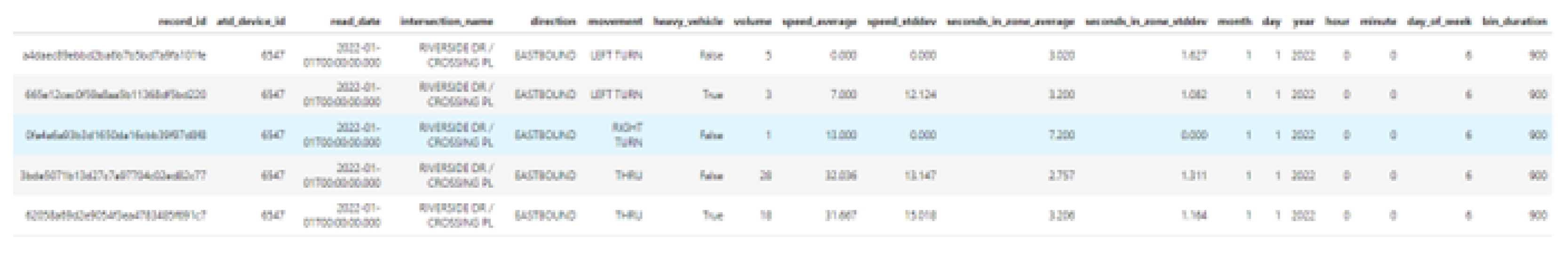
In this paper, a Camera Traffic Count from the city of Austin, Texas, is used. This is a public dataset collected from the City of Austin’s Open Data Portal (https://data.austintexas.gov/Transportation-and-Mobility/Camera-Traffic-Counts/sh59-i6y9/data). The dataset contains traffic counts for 68 intersections in the form of flow time series and speeds for 15-minute intervals starting from June 2017 till the time of this paper, August 2022. As illustrated in Figure 2, the dataset labels traffic volume based on the intersection, direction (such as southbound or eastbound), movement (like left turn or thru), vehicle size, average speed, and date-time.
Due to the large size of data available, this paper will be using traffic data for one intersection starting from January 2022 till August 2022.
2.1. Data Preprocessing
It is good practice to assume the possibility of missen values caused by intermittent camera or sensor failures. Using simple imputation, as explained by [8], missing data can be filled with the historical average, mode, mean, or median of the available values. However, in high-dimensional data sets, simplistic imputation techniques might lead to inaccurate or unrealistic outcomes. In our experiment, missen fields weren’t encountered; rather, the dataset did not have records where traffic volume was zero.
This study focuses on federated machine learning, but centralized learning where also conducted as the control.
Using the Python pandas library, all 2022 records for one intersection is loaded. The data at this point has no DateTime column; rather, it has month, day, hour, and minute. A DateTime column is created for all records using these. As shown in Figure 2, the traffic volumes for heavy and light vehicles are recorded separately. Since the scope of this study does not account for vehicle size classification, the data is grouped by intersection name, direction, movement, and DateTime then the corresponding traffic volumes are aggregated while unnecessary columns are dropped. Using LabelEncoder from the Scikit-learn library, all non-numerical columns are encoded into numerical equivalence in new columns. Furthermore, the data is randomly rearranged.
Before the data is used for building models, the volume column is taken as the output ’Y’ while every other numerical column is scaled using StandardScaler from the Scikit-learn library and then used as the input ’X’.
2.2. Machine Learning Methods
In this paper, five regression models, namely Stochastic Gradient Descendent Regressor, Linear Regression, Gradient Boosting Regressor, Random Forest Regressor, and MultiLayer Perceptron Regressor, are used to prove the performance of federated learning when compared with centralized learning for traffic prediction.
2.2.1. Centralized Learning
It is a machine learning implementation where the data, model, and evaluation happen on the same machine. The usual procedure is to gather data across edge devices and train a statistical model with them. This method is referred to as centralized learning.
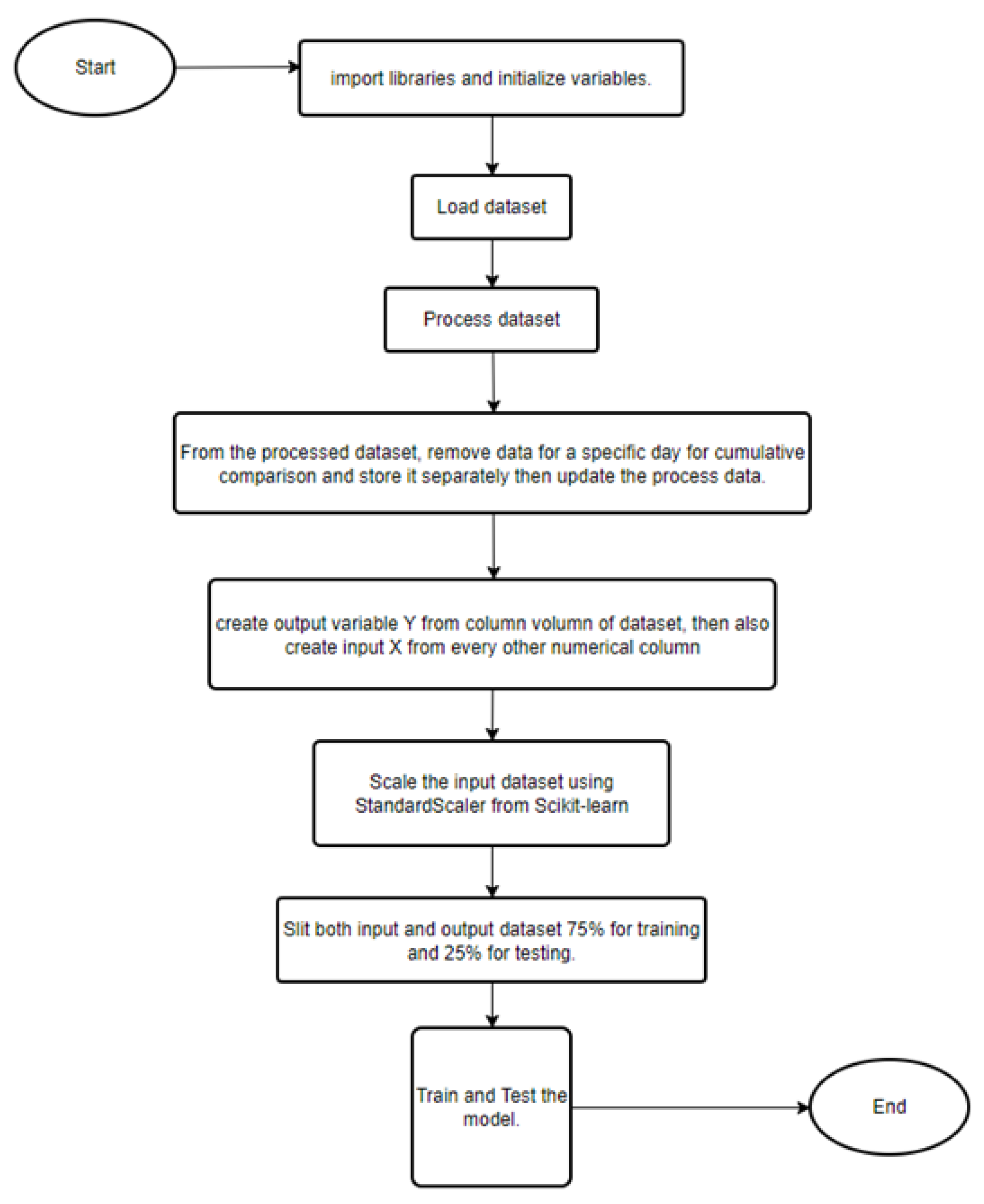
A centralized learning algorithm was implemented using each of the five machine learning models. The following flowchart shows the sequence in which centralized learning was done.
Figure 3.
Flowchart of centralized learning method implementation.
2.2.2. Federated Learning
Data privacy is ignored in centralized machine learning while federated machine learning ensures that actual data is not shared. Federated learning, in simple terms, is decentralized machine learning without sharing data. It ensures the training of statistical models over edge devices while keeping data localized[9]. To perfectly aggregate data from federated learning, strategies like Federated Averaging[10] or Federated Optimization[11] are commonly used.
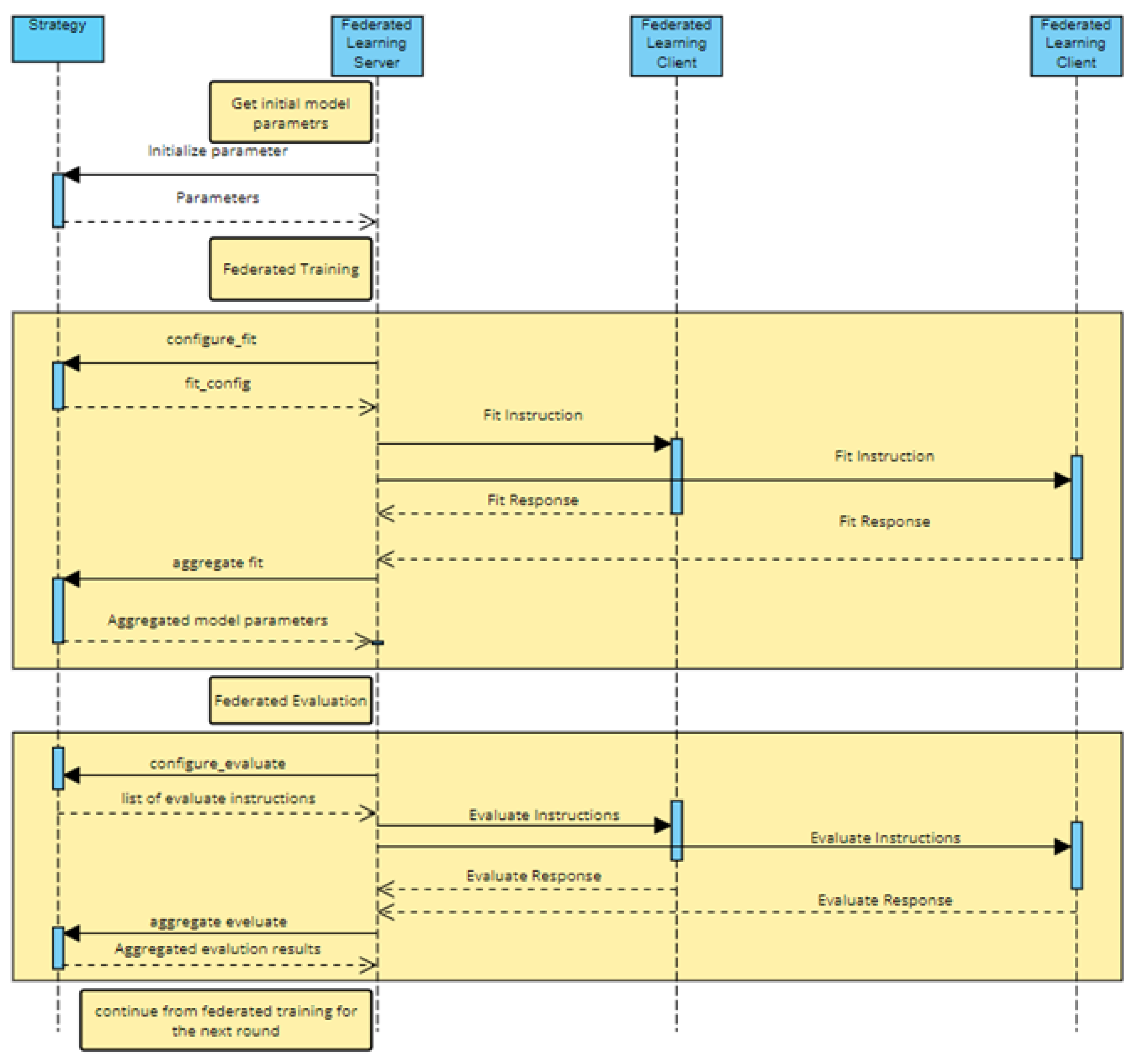
To perform federated learning, the Python library Flower was used. The federated learning procedure requires three parts to function, namely Strategy, Federated Learning Server, and at least 2 Federated Learning Clients.
The strategy used for this federated learning was Federated Optimization, and the preprocessed data was split across the Federated Learning Clients. A variation of 2 to 10 Federated Learning clients was used while performing five training and evaluation rounds.
2.2.3. Relevant Machine Learning Models
Linear Regression
A statistical technique called linear regression is used to examine the correlation between a dependent variable and one or more independent variables. It is a method that is frequently employed to forecast continuous numerical values.
In linear regression, the connection between the dependent variable and the independent variables is shown as a straight line, sometimes referred to as the regression line. For a specific collection of independent variables, the dependent variable’s value is estimated using the regression line. Finding the equation of the line that best fits the data points is the fundamental concept of linear regression. Mathematically Linear Regression can be represented by the following equation;
where,
y = Variable y is an output that represents the continuous value that the model tries to predict.
x = input variable. In machine learning, x is the feature, while it is termed the independent variable in statistics. Variable x represents the input information provided to the model at any given time.
P0 = y-axis intercept (or the bias term).
P1 = the regression coefficient or scale factor. In classical statistics, P1 is the equivalent of the slope of the best-fit straight line of the linear regression model.
Gradient Boosting Regressor
In general, boosting is a technique that involves the combination of multiple simple models to produce an ensemble[12]. Boosting’s central tenet is the sequential introduction of new models into the ensemble. A new, low-power base-learner model is taught at each iteration based on the error of the previously learned ensemble as a whole. Gradient Boosting Regress involves three elements, namely loss function to be optimized, a weak learner to make predictions, and an additive model to add weak learners to minimize the loss function[12].
MultiLayer Perceptron Regressor
An artificial neural network called a multi-layer perceptron has at least three layers of perceptrons. In addition to its input and output layers, a Multi-layer Perceptron often comprises one or more hidden layers that contain a large number of neurons. And although the activation function of a neuron in a Perceptron must impose a threshold in some way (via methods like ReLU or sigmoid), a Multi-layer Perceptronś neurons are free to employ whatever activation function they wish[13].
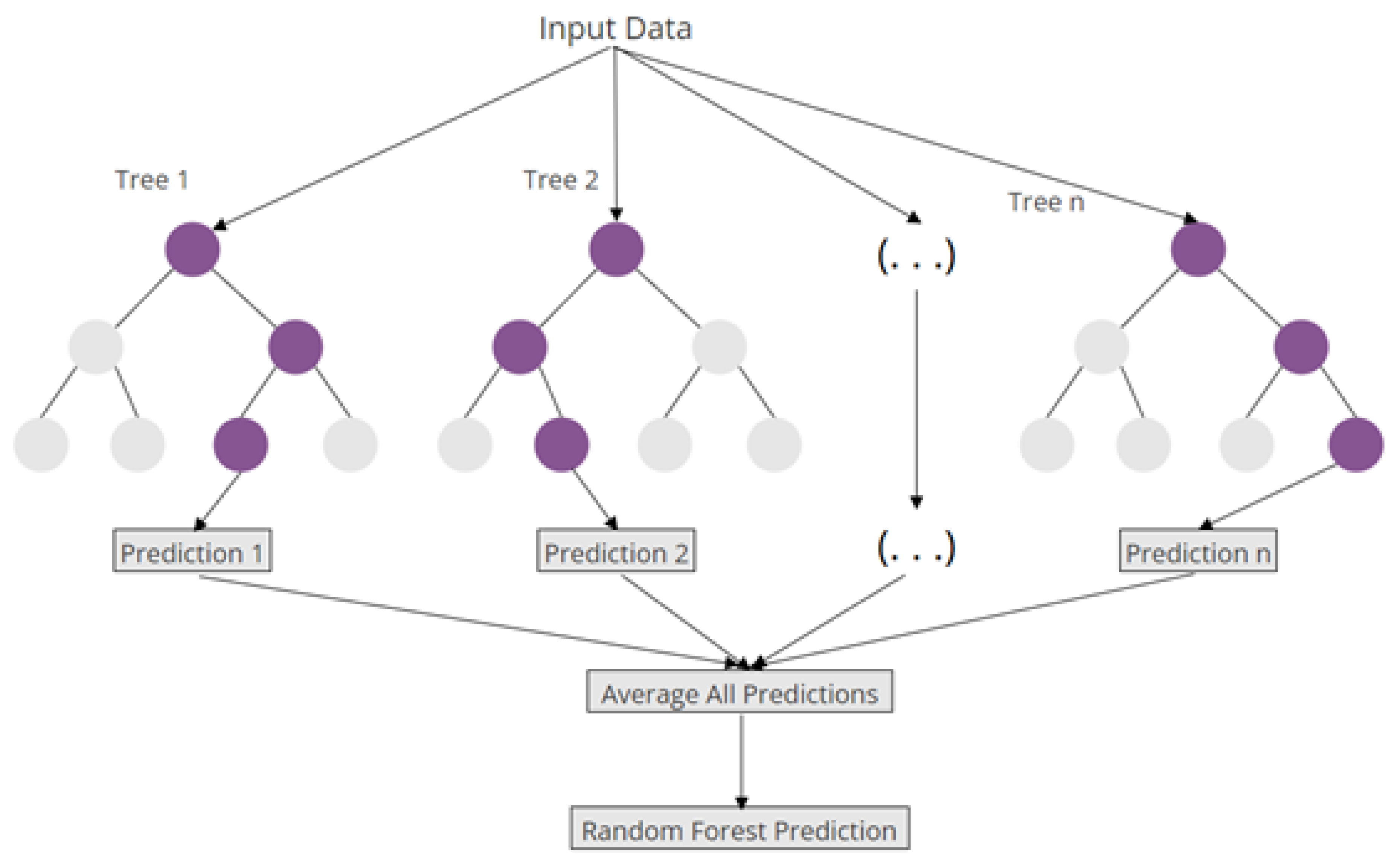
Random Forest Regressor
This regressor is a supervised learning algorithm that uses an ensemble learning technique. The predictions of numerous machine learning algorithms are combined in an ensemble learning approach to provide a more precise forecast than any one model could on its own.
Stochastic Gradient Decent Regressor
The SGD Regressor is a machine-learning technique that employs stochastic gradient descent to make predictions. This algorithm takes a dataset as input and uses its gradient descent algorithm to determine the best-fit line that runs through the data and then makes predictions based on this line. The algorithm is iterative, with each iteration improving the accuracy of the fit line. Compared to other linear regression algorithms, the SGD Regressor is faster, making it ideal for large datasets. Additionally, it works well with sparse datasets because it can ignore irrelevant features. However, the SGD Regressor is sensitive to scaling, so it is crucial to scale the data before using the algorithm. Furthermore, it may overfit if not used appropriately.
2.2.4. Performance Metrics
To make a proper comparison between centralized machine learning and federated learning, mean absolute error (MAE), relative squared error(RSE), root mean squared error(RMSE), and mean absolute performance error(MAPE).
Mean Absolute Error (MAE):
Mean absolute error or L1 loss is a straightforward statistic for judging model performance. It is determined by averaging the absolute differences between the predicted and actual values across the dataset.
where = actual value, = predicted value, and n = sample size
Mean Absolute Performance Error (MAPE):
By dividing the difference between the actual and anticipated values by the actual value, we can get the mean absolute percentage error. This number is multiplied by an absolute percentage and then averaged across the whole dataset.
where = actual value, = predicted value, and n = sample size
Root Mean Squared Error (RMSE):
By calculating the square root of the mean squared error (MSE), RMSE is calculated. To be clear, MSE is determined by squaring the difference between the projected value and the actual value and then average it throughout the dataset. RMSE measures the average magnitude of the errors and is concerned with the deviations from the actual value. A zero value of RMSE indicates that the model has a perfect fit.
where = actual value, = predicted value, and n = sample size
Relative Squared Error (RSE):
RSE is determined by dividing Mean Squared Error (MSE) by the squared of the difference between the mean and the actual of the data.
where = actual value, = predicted value, n = sample size, and ,
3. Results
To evaluate the performance of both Centralized and Federated machine learning models, metrics such as mean absolute error (MAE), explained variance (EV), root mean square error (RMSE), R-squared (R2), and mean absolute percentage error (MAPE) was gotten using the Scikit-learn library.
Since time is an important factor in determining how applicable in a real-world scenario, the execution time of all the models was measured. As expected, the centralized machine learning models have a significantly short execution time when compared to the federated learning models. This is explainable considering network latency and the five rounds of training and execution time in the federated machine learning models.
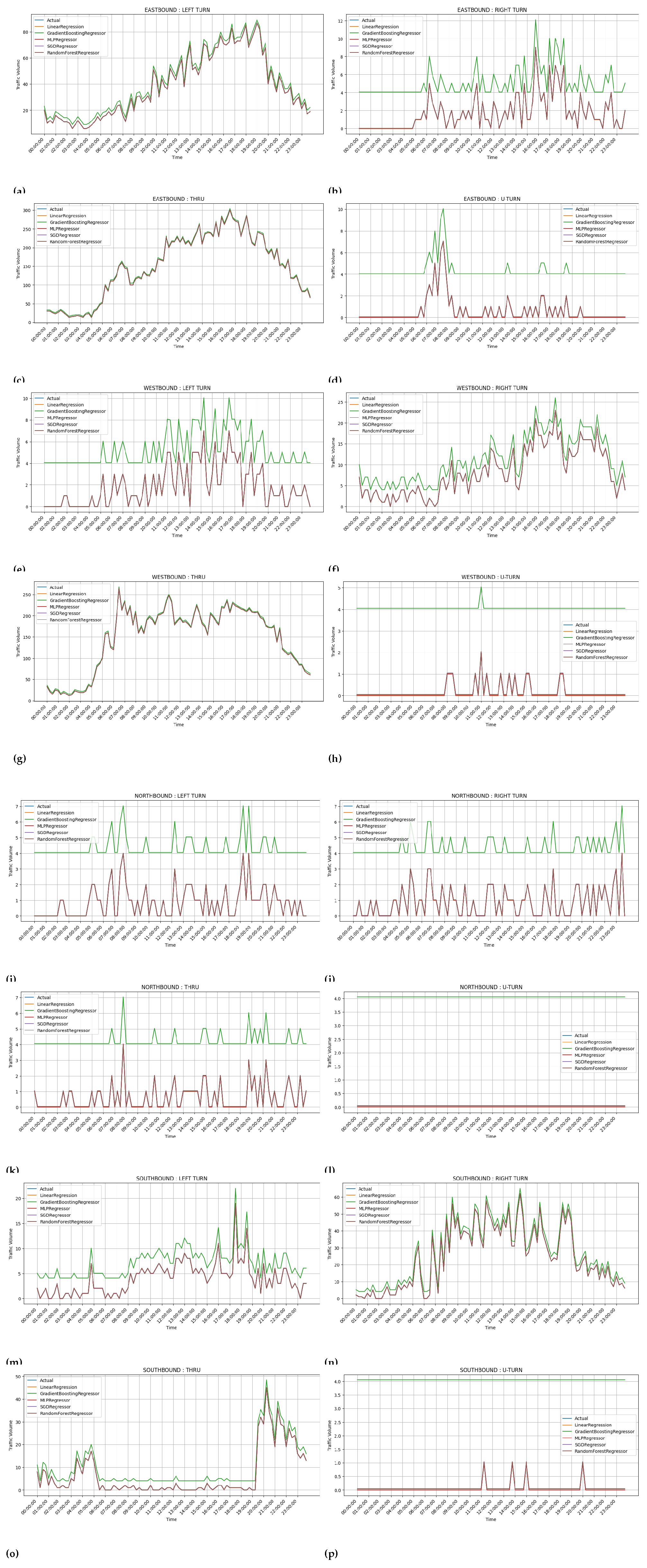
In addition, to analyze how effective the models are in predicting the actual values, the single-day data removed after preprocessing was used to get a one-day prediction from each model in centralized and federated machine learning. The prediction results were compared with the actual traffic volume, and the line plot below shows a more precise picture beyond the metrics of each model.
4. Discussion
The tables and figures on traffic prediction model provide detailed information on the comparison of centralized and federated training. These are examined in the followig with reference to specific table or figure:
4.1. Table 1: Centralized Learning Metrics
-
Key Observations:
- –
- Models such as MLP Regressor, SGD Regressor, and Random Forest Regressor seem to give impressive performance (R² score of 1.0, MAEs and RMSEs are 0 or nearly 0).
- –
- The time needed by Linear Regression was the fastest (0.0237 seconds); therefore, the model was the worst compared to the others regarding all performance factors.
- –
- Gradient Boosting Regressor was not bad in execution time (3.206 s) and had somewhat higher error readings (i.e., MAE = 0.1423) in comparison to MLP, SGD, and Random Forest Regressors.
-
Implications:
- –
- Centralized learning is very fast, but it is quite inflexible and falls short of the current privacy and decentralization requirements in modern systems.
- –
- Models such as Random Forest and SGD Regressors have a good balance of low error measures along with fair execution times to be practical choices.

Table 1.
Comparison of performance metrics using centralized learning.
| Model | Time(Sec) | EV | R2 | MAE | RMSE | MAPE |
|---|---|---|---|---|---|---|
| Linear Regression | 0.023708 | 1.000000 | 1.000000 | 0.000000 | 0.000000 | 0.000000 |
| Gradient Boosting Regressor | 3.206007 | 0.999976 | 0.999976 | 0.142326 | 0.296681 | 0.006360 |
| MLP Regressor | 2.555572 | 1.000000 | 1.000000 | 0.000001 | 0.000002 | 0.000000 |
| SGD Regressor | 0.072035 | 1.000000 | 1.000000 | 0.004492 | 0.006381 | 0.001243 |
| RandomForestRegressor | 4.593522 | 1.000000 | 1.000000 | 0.000099 | 0.007171 | 0.000000 |
4.2. Table 2, Table 3, Table 4 and Table 5: Federated Learning Metrics (2 to 5 Clients)
-
Key Observations:
- –
- R² and EV values are kept consistently high for all models and configurations throughout all tables with value .
- –
- Execution times increased with an increasing number of clients, an example is MLP Regressor time values, which were 208 seconds for 2 clients and 411 seconds for 5 clients.
- –
- Linear Regression demonstrated increasing MAE and RMSE values as the count of clients increased. This shows its inefficiency in a distributed system.
- –
- Random Forest and SGD Regressors managed to maintain low MAE values of the order of 0.0046 across all five clients, with moderate time consumption of about 17 sec for 5 clients.
-
Implications:
- –
- It is possible for federated learning to scale with the number of clients while maintaining predictive accuracy.
- –
- For a real-time decentralized traffic management system, the SGD Regressor and Random Forest regressor have reasonable trade-off between accuracy and reasonable execution times.
Table 2.
Comparison of performance metrics using two clients in federated learning.
| Model | Time(Sec) | EV | R2 | MAE | RMSE | MAPE |
|---|---|---|---|---|---|---|
| Linear Regression | 15.326317 | 0.999996 | 0.999994 | 0.081291 | 0.146484 | 0.004795 |
| Gradient Boosting Regressor | 31.233635 | 0.999974 | 0.999974 | 0.146348 | 0.315305 | 0.006466 |
| MLP Regressor | 208.376528 | 1.000000 | 1.000000 | 0.000000 | 0.000001 | 0.000000 |
| SGD Regressor | 15.075476 | 1.000000 | 1.000000 | 0.004635 | 0.006648 | 0.001276 |
| Random Forest Regressor | 15.208890 | 1.000000 | 1.000000 | 0.004771 | 0.006879 | 0.001295 |
Table 3.
Comparison of performance metrics using three clients in federated learning.
| Model | Time(Sec) | EV | R2 | MAE | RMSE | MAPE |
|---|---|---|---|---|---|---|
| Linear Regression | 15.687742 | 0.999985 | 0.999964 | 0.265519 | 0.347557 | 0.047209 |
| Gradient Boosting Regressor | 26.090589 | 0.999972 | 0.999972 | 0.144553 | 0.319226 | 0.006544 |
| MLP Regressor | 274.414383 | 1.000000 | 1.000000 | 0.000000 | 0.000001 | 0.000000 |
| SGD Regressor | 16.625714 | 1.000000 | 1.000000 | 0.004580 | 0.006529 | 0.001285 |
| Random Forest Regressor | 16.510526 | 1.000000 | 1.000000 | 0.004641 | 0.006676 | 0.001283 |
Table 4.
Comparison of performance metrics using four clients in federated learning.
| Model | Time(Sec) | EV | R2 | MAE | RMSE | MAPE |
|---|---|---|---|---|---|---|
| Linear Regression | 17.035590 | 0.999990 | 0.999982 | 0.154584 | 0.224460 | 0.023374 |
| Gradient Boosting Regressor | 25.258733 | 0.999972 | 0.999972 | 0.147918 | 0.320299 | 0.006366 |
| MLP Regressor | 360.875556 | 1.000000 | 1.000000 | 0.000000 | 0.000001 | 0.000000 |
| SGD Regressor | 17.343573 | 1.000000 | 1.000000 | 0.004573 | 0.006604 | 0.001256 |
| Random Forest Regressor | 16.577347 | 1.000000 | 1.000000 | 0.004554 | 0.006520 | 0.001271 |
Table 5.
Comparison of performance metrics using five clients in federated learning.
| Model | Time(Sec) | EV | R2 | MAE | RMSE | MAPE |
|---|---|---|---|---|---|---|
| Linear Regression | 18.032668 | 0.999989 | 0.999980 | 0.144827 | 0.214542 | 0.021945 |
| Gradient Boosting Regressor | 24.101755 | 0.999974 | 0.999974 | 0.148933 | 0.312832 | 0.006453 |
| MLP Regressor | 410.924955 | 1.000000 | 1.000000 | 0.000001 | 0.000001 | 0.000000 |
| SGD Regressor | 17.343014 | 1.000000 | 1.000000 | 0.004627 | 0.006614 | 0.001283 |
| Random Forest Regressor | 17.813065 | 1.000000 | 1.000000 | 0.004662 | 0.006695 | 0.001289 |
4.3. Figure 4: Cumulative Execution Time Comparison
-
Key Observations:
- –
- Federated learning had higher execution times than their centralized learning, due largely to network communications and synchronization overhead.
- –
- Execution times spike for a majority of MLP Regressors by such an average of 41% as the number of clients increased from 2 clients at 208 seconds to 5 clients, attaining over 400 seconds.
- –
- SGD and Random Forest Regressors deliver moderate-time executions across client counts and show strong efficiency to scale.
-
Implications:
- –
- In time to execute vs scalability, it is absolutely essential to try to reduce the latency of communication protocols while maintaining predictive quality.
Figure 4.
Sequence Diagram for the federating learning implementation.
4.4. Figure 5: Execution Time of Individual Models
-
Key Observations:
- –
- Linear Regression encountered the lowest execution time in both cases, with a further decline in prediction quality for a federated setup.
- –
- MLP Regressor, having excelled in metrics, cannot be applied to real-time systems because of their long execution.
- –
- SGD and Random Forest Regressors require a constant, modest execution time in both cases, centralized or federated.
-
Implications:
- –
- Real-time application thus becomes a crucial parameter for both regression times, and at this, SGD and Random Forest Regressors serve as relatively well-balanced solutions, specially in federated learning situations.
Figure 5.
Structure of a Random Forest.
4.5. Figure 6, Figure 7, Figure 8 and Figure 9: Prediction Accuracy for Various Configurations
-
Key Observations:
- –
- The figures capture predicted traffic flow against actuals for various driving patterns and directions ( notably left turns on the eastbound and right turns on the westbound, respectively).
- –
- –
- The increase of client numbers did not perceptibly affect the prediction accuracy regardless of any issue.
-
Implications:
- –
- Federated learning systems scale with considerable success yet continue to deliver the highest prediction accuracy, making them apt for a real-life application on traffic modelling.
- –
- Similarly minor deviations in Linear Regression indicate limited predictive power just in comparison to other models.
Figure 6.
A cumulative comparison of execution time for both centralized learning(CL) and distributed federated learning(FL) with multiple clients.
Figure 6.
A cumulative comparison of execution time for both centralized learning(CL) and distributed federated learning(FL) with multiple clients.
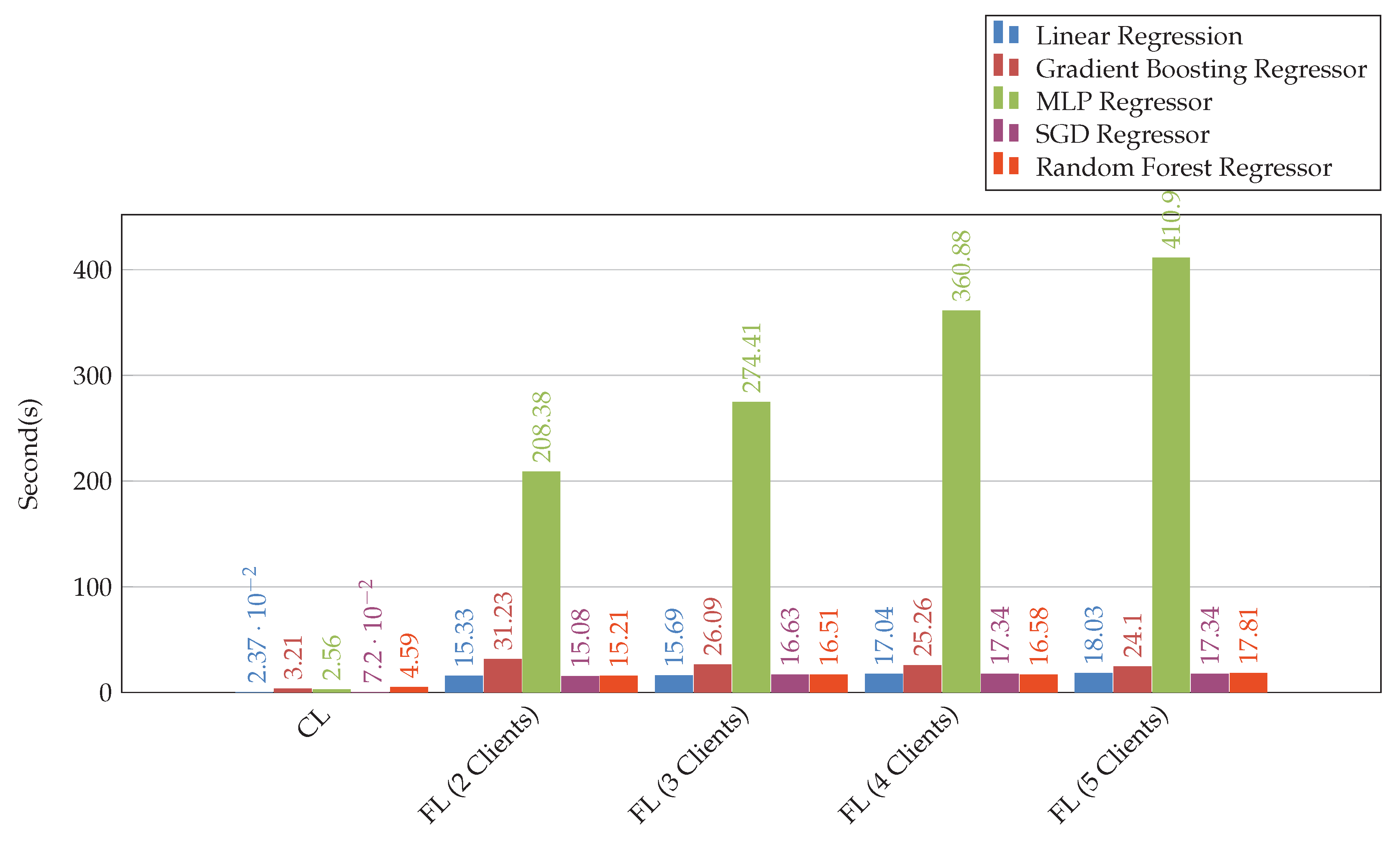
Figure 7.
Comparison of execution time for all the prediction models. (a) Execution time for all cases of Linear Regression; (b) Execution time for all cases of Gradient Boost Regressor; (c) Execution time for all cases of Multi-layer Perceptron Regressor; (d) Execution time for all cases of Stochastic Gradient Descent Regressor; (e) Execution time for all cases of Random Forest Regressor.
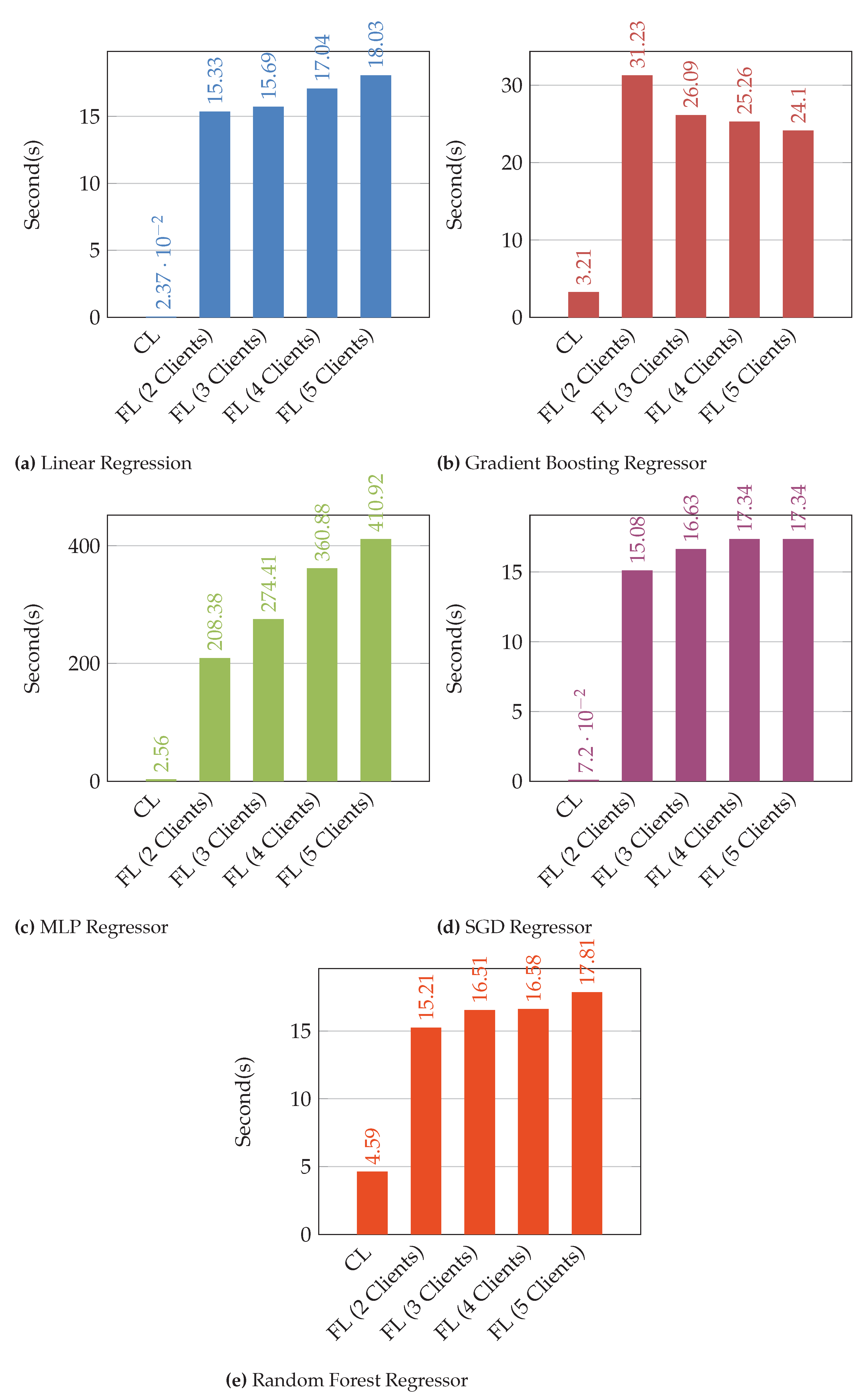
Figure 8.
Comparison of centralized learning traffic flow prediction for movements in all directions at an intersection for one test day. (a)Eastbound left turn traffic prediction; (b)Eastbound right turn traffic prediction; (c)Eastbound through traffic prediction; (d)Eastbound u-turn traffic prediction; (e)Westbound left turn traffic prediction; (f)Westbound right turn traffic prediction; (g)Westbound through traffic prediction; (h)Westbound u-turn traffic prediction; (i)Northbound left turn traffic prediction; (j)Northbound right turn traffic prediction; (k)Northbound through traffic prediction; (l)Northbound u-turn traffic prediction; (m)Southbound left turn traffic prediction; (n)Southbound right turn traffic prediction; (o)Southbound through traffic prediction; (p)Southbound u-turn traffic prediction.
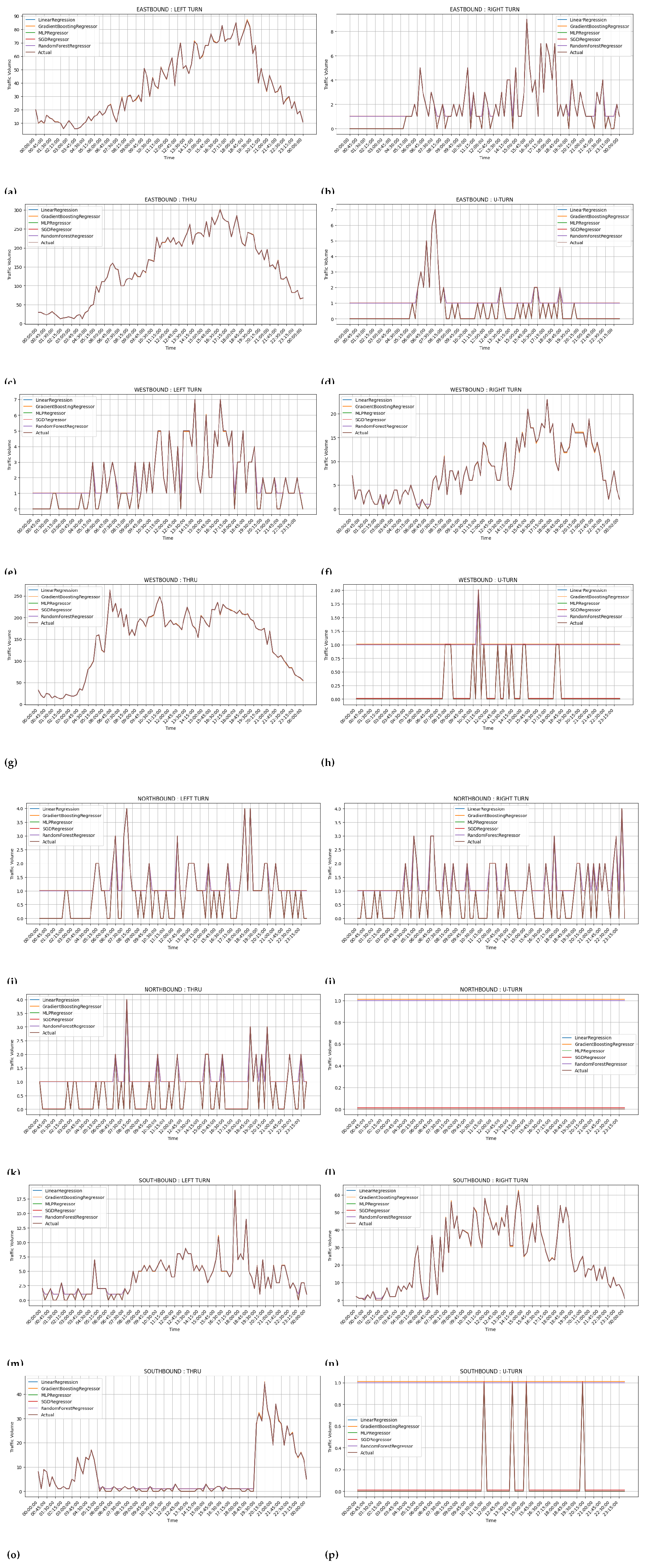
Figure 9.
Comparison of federated learning traffic flow prediction for movements in all directions at an intersection with two clients for one test day. (a)Eastbound left turn traffic prediction; (b)Eastbound right turn traffic prediction; (c)Eastbound through traffic prediction; (d)Eastbound u-turn traffic prediction; (e)Westbound left turn traffic prediction; (f)Westbound right turn traffic prediction; (g)Westbound through traffic prediction; (h)Westbound u-turn traffic prediction; (i)Northbound left turn traffic prediction; (j)Northbound right turn traffic prediction; (k)Northbound through traffic prediction; (l)Northbound u-turn traffic prediction; (m)Southbound left turn traffic prediction; (n)Southbound right turn traffic prediction; (o)Southbound through traffic prediction; (p)Southbound u-turn traffic prediction.
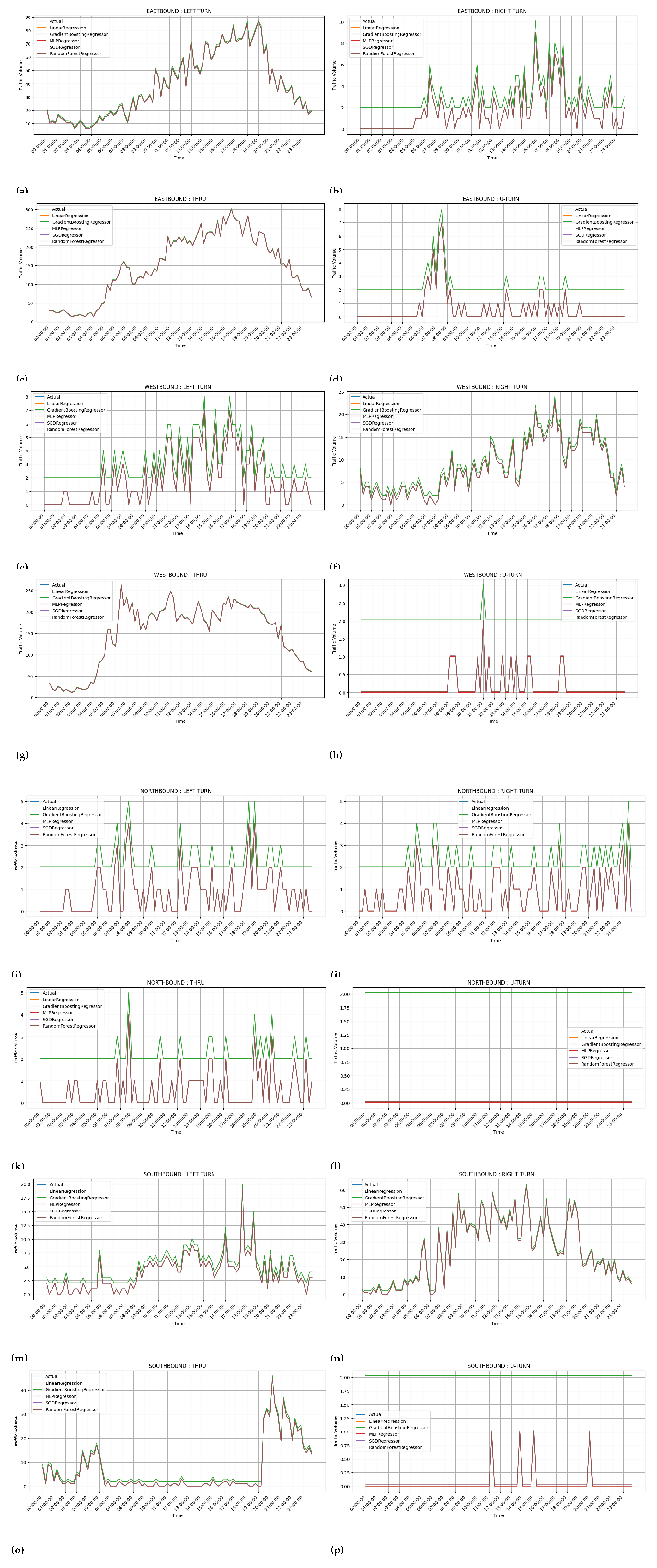
Figure 10.
Comparison of federated learning traffic flow prediction for movements in all directions at an intersection with three clients for one test day. Comparison of federated learning traffic flow prediction for movements in all directions at an intersection with three clients for one test day. (a)Eastbound left turn traffic prediction; (b)Eastbound right turn traffic prediction; (c)Eastbound through traffic prediction; (d)Eastbound u-turn traffic prediction; (e)Westbound left turn traffic prediction; (f)Westbound right turn traffic prediction; (g)Westbound through traffic prediction; (h)Westbound u-turn traffic prediction; (i)Northbound left turn traffic prediction; (j)Northbound right turn traffic prediction; (k)Northbound through traffic prediction; (l)Northbound u-turn traffic prediction; (m)Southbound left turn traffic prediction; (n)Southbound right turn traffic prediction; (o)Southbound through traffic prediction; (p)Southbound u-turn traffic prediction.
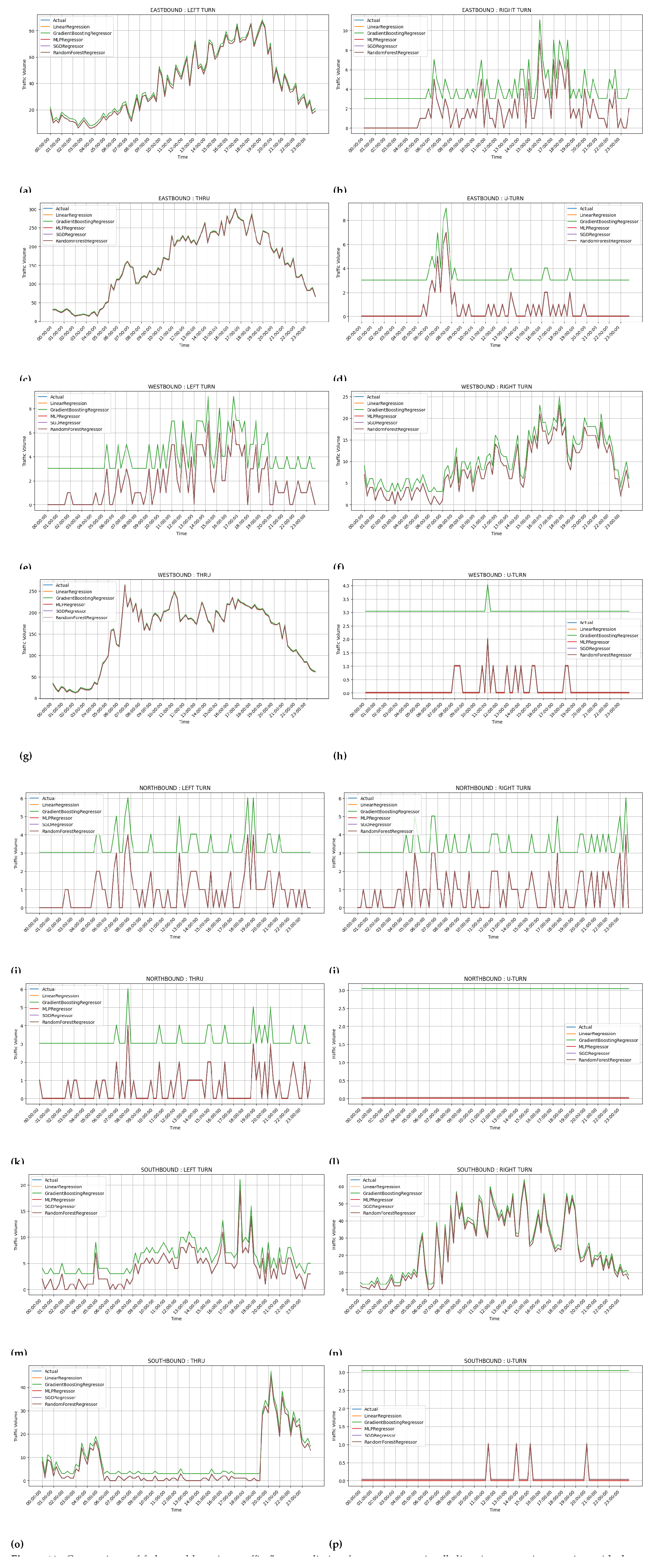
Figure 11.
Comparison of federated learning traffic flow prediction for movements in all directions at an intersection with four clients for one test day. (a)Eastbound left turn traffic prediction; (b)Eastbound right turn traffic prediction; (c)Eastbound through traffic prediction; (d)Eastbound u-turn traffic prediction; (e)Westbound left turn traffic prediction; (f)Westbound right turn traffic prediction; (g)Westbound through traffic prediction; (h)Westbound u-turn traffic prediction; (i)Northbound left turn traffic prediction; (j)Northbound right turn traffic prediction; (k)Northbound through traffic prediction; (l)Northbound u-turn traffic prediction; (m)Southbound left turn traffic prediction; (n)Southbound right turn traffic prediction; (o)Southbound through traffic prediction; (p)Southbound u-turn traffic prediction.
4.6. Overall Discussion:
-
Accuracy vs. Execution Time:
- –
- Regardless of client count, federated learning models always had a high rate of accuracy (Table 2, Table 3, Table 4 and Table 5 and Figure 6, Figure 7, Figure 8 and Figure 9), while execution time increased with more clients as in Figure 4 thereby making the MLP unsuitable for practical applications.
-
Model Selection:
- –
- From results on all the tables and figures, we can see that Random Forest and SGD Regressors provide just the right balance between execution time and accuracy.
- –
- Though otherwise a good conclusion can be drawn about the MLP Regressor, it offers accuracy but is not the best for real-time applications due to its high computational overhead.
-
Federated Learning Scalability:
- –
- Tables and Figures showed on average that federated learning scales well. It maintained high accuracy as clients increased despite longer execution times.
-
Practical Implications for Virtual Traffic Lights:
- –
- Federated Learning systems provide accurate, decentralized, and privacy-preserving framework for traffic prediction.
- –
- With optimized execution times, these systems may support real-time applications like virtual traffic lights.
5. Conclusion
In this paper, we proposed several federated machine learning models for traffic flow prediction for direction (such as southbound or eastbound) and movement (like left turn or through) at intersections. This paper lays a working groundwork for virtual traffic lights. One traffic dataset from the City of Austin’s Open Data Portal was used to train, validate and test the proposed models. Overall, from an amalgamated interpretation of tables and figures, it is seen that the federated learning models, especially Random Forest and SGD regressors, are one of the best shooters for decentralized traffic prediction systems. While balking the problem of the execution time, their scalability and accuracy are logically becoming the strong contenders for applications of virtual traffic lights. Although MLP Regressor had the best metric performance, its slow execution time makes it unusable for the proposed virtual traffic lights. Gradient Boosting Regressor consistently had the second worst execution time and also performed poorly on MAE, RMSE, and MAPE metrics. Finally, Linear Regression had a faster execution time when compared to Gradient Boosting Regressor, but it also performed poorly on MAE, RMSE, and MAPE metrics. In general, all the federated machine learning models with an increasing number of clients had an explainable variance and an R2 greater than 0.999. In conclusion, the results show that federated machine learning satisfactorily predicted traffic flow in all directions at an intersection, and this demonstrates how feasible it is to implement virtual traffic lights, as proposed in Figure 1.1.
Funding
This research received no external funding.
Institutional Review Board Statement
Not applicable.
Informed Consent Statement
Not applicable.
Data Availability Statement
Data are available at:https://data.austintexas.gov/Transportation-and-Mobility/Camera-Traffic-Counts/sh59-i6y9/data (January 2022 till August 2022 dataset).
Acknowledgments
I want to express my sincere gratitude and appreciation to my thesis committee for their invaluable guidance, support, and contribution throughout my academic journey.
First and foremost, I would like to extend my heartfelt thanks to my thesis committee chair, Hardik Gohel (Ph.D.), for his unwavering support, insightful feedback, and invaluable guidance throughout the thesis process. I am deeply grateful for his patience, dedication, and enthusiasm for my research project.
Lastly, I thank my family and friends for their unconditional love, support, and encouragement. Without their constant motivation, this achievement would not have been possible.
Conflicts of Interest
The authors declare no conflicts of interest.
References
- Elbir, A.M.; Soner, B.; Coleri, S.; Gunduz, D.; Bennis, M. Federated Learning in Vehicular Networks, 2020, [arXiv:cs.NI/2006.01412].
- Feng, H.; Shu, Y. Study on Network Traffic Prediction Techniques. In Proceedings of the Proceedings - 2005 International Conference on Wireless Communications, Networking and Mobile Computing (WCNM 2005), 2005, Vol. 2, pp. 995–998. [CrossRef]
- George, S.; Santra, A.K. Traffic Prediction Using Multifaceted Techniques: A Survey. Wireless Personal Communications 2020, 115. [Google Scholar] [CrossRef]
- Li, J.; Boonaert, J.; Doniec, A.; Lozenguez, G. Multi-Models Machine Learning Methods for Traffic Flow Estimation from Floating Car Data. Transportation Research Part C: Emerging Technologies 2021, 132. [Google Scholar] [CrossRef]
- Alam, I.; Md. Farid, D.; Rossetti, R.J.F. The Prediction of Traffic Flow with Regression Analysis. In Emerging Technologies in Data Mining and Information Security; Springer, Singapore, 2019; Vol. 813, Advances in Intelligent Systems and Computing. [CrossRef]
- Zhang, R.; Schmutz, F.; Gerard, K.; Pomini, A.; Basseto, L.; Hassen, S.b.; Ishikawa, A.; Ozgunes, I.; Tonguz, O. Virtual Traffic Lights: System Design and Implementation, 2018, [arXiv:cs.NI/1807.01633].
- Ekmefjord, M.; Ait-Mlouk, A.; Alawadi, S.; Akesson, M.; Singh, P.; Spjuth, O.; Toor, S.; Hellander, A. Scalable Federated Machine Learning with FEDn. In Proceedings of the Proceedings - 22nd IEEE/ACM International Symposium on Cluster, Cloud and Internet Computing (CCGrid 2022), 2022, pp. 555–564. [CrossRef]
- Emmanuel, T.; Maupong, T.; Mpoeleng, D.; Semong, T.; Mphago, B.; Tabona, O. A Survey on Missing Data in Machine Learning. Journal of Big Data 2021, 8. [Google Scholar] [CrossRef] [PubMed]
- Li, T.; Sahu, A.K.; Talwalkar, A.; Smith, V. Federated Learning: Challenges, Methods, and Future Directions. IEEE Signal Processing Magazine 2020, 37. [Google Scholar] [CrossRef]
- McMahan, H.B.; Moore, E.; Ramage, D.; Hampson, S.; Arcas, B.A.y. Communication-Efficient Learning of Deep Networks from Decentralized Data, 2016, [arXiv:cs.LG/1602.05629].
- Li, T.; Sahu, A.K.; Zaheer, M.; Sanjabi, M.; Talwalkar, A.; Smith, V. Federated Optimization in Heterogeneous Networks, 2018, [arXiv:cs.LG/1812.06127].
- Keprate, A.; Ratnayake, R.M.C. Using Gradient Boosting Regressor to Predict Stress Intensity Factor of a Crack Propagating in Small Bore Piping. In Proceedings of the IEEE International Conference on Industrial Engineering and Engineering Management, 2017. [CrossRef]
- Vaswani, A.; Shazeer, N.; Parmar, N.; Uszkoreit, J.; Jones, L.; Gomez, A.N.; Kaiser, L.u.; Polosukhin, I. Attention is All you Need. In Proceedings of the Advances in Neural Information Processing Systems; Guyon, I.; Luxburg, U.V.; Bengio, S.; Wallach, H.; Fergus, R.; Vishwanathan, S.; Garnett, R., Eds. Curran Associates, Inc., 2017, Vol. 30.
Figure 1.
Flowchart of Virtual traffic light algorithm with federated machine learning.
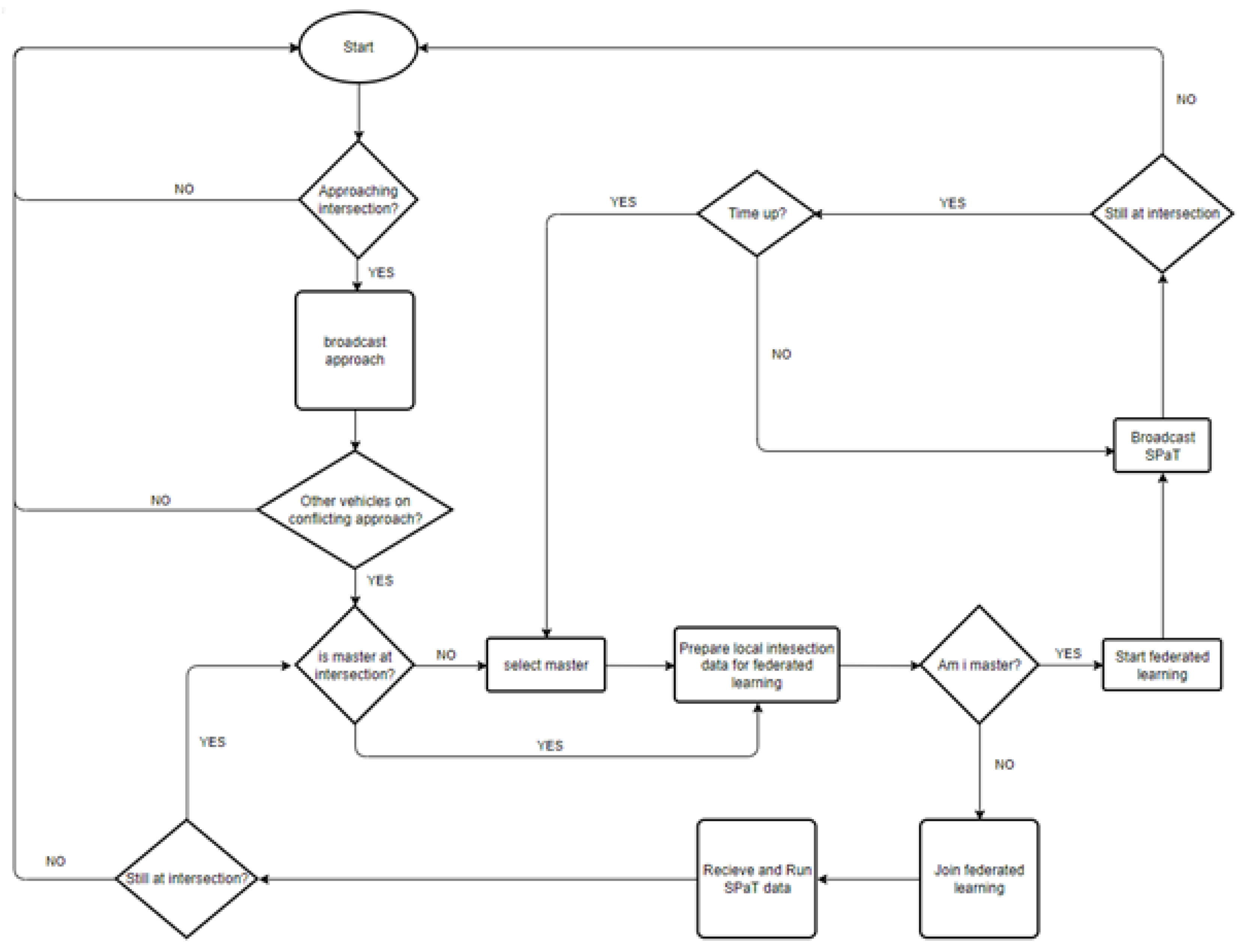
Figure 2.
Data Sample.
Disclaimer/Publisher’s Note: The statements, opinions and data contained in all publications are solely those of the individual author(s) and contributor(s) and not of MDPI and/or the editor(s). MDPI and/or the editor(s) disclaim responsibility for any injury to people or property resulting from any ideas, methods, instructions or products referred to in the content. |
© 2025 by the authors. Licensee MDPI, Basel, Switzerland. This article is an open access article distributed under the terms and conditions of the Creative Commons Attribution (CC BY) license (http://creativecommons.org/licenses/by/4.0/).
Copyright: This open access article is published under a Creative Commons CC BY 4.0 license, which permit the free download, distribution, and reuse, provided that the author and preprint are cited in any reuse.


