

Submitted:
28 July 2025
Posted:
30 July 2025
You are already at the latest version
Abstract
Maritime safety, environmental protection and efficient traffic management increasingly rely on data-driven technologies. However, leveraging Automatic Identification System (AIS) data for predictive modelling faces two major challenges: the massive volume of data generated in real-time and growing privacy concerns associated with proprietary vessel information. This paper proposes a novel, privacy-preserving framework for vessel traffic density (VTD) prediction that addresses both challenges. The approach combines EMODNet’s grid-based VTD calculation method with Convolutional Neural Networks (CNN) to model spatiotemporal traffic patterns and employs Federated Learning to collaboratively build a global predictive model without the need for explicit sharing of proprietary AIS data. Three geographically diverse AIS datasets were harmonized, processed, and used to train local CNN models on hourly VTD matrices. These models were then aggregated via a Federated Learning framework, under a lifelong learning scenario. Evaluation using Sparse Mean Squared Error (Sparse MSE) shows that the federated global model achieves promising accuracy in sparse data scenarios and maintains performance parity when compared with local CNN-based models, all while preserving data privacy and minimizing hardware performance needs and data communication overheads. The results highlight the approach’s effectiveness and scalability for real-world maritime applications in traffic forecasting, safety, and operational planning.
Keywords:
vessel traffic density
; federated learning
; convolutional neural networks
; artificial intelligence
; maritime logistics
; automatic identification system
1. Introduction
1.1. Context and Motivation
Since ancient times, the maritime domain has been vital as a hub for communication, travel, and trade, driving cultural exchange, economic growth, and the global movement of goods and people [1]. Today, it plays an even more crucial role in global trade, security, and environmental sustainability. Over 80% of global trade by volume is now transported via maritime routes, supported by a fleet of over 50,000 merchant vessels. In 2022 alone, container carriers earned an estimated $296.3 billion, a 38% increase from 2021 [2].
Despite these benefits, the scale of maritime activity brings major challenges. According to the 2022 United Nations Conference on Trade and Development (UNCTAD) report port congestion increased significantly, especially in China, the U.S., and Northern Europe, where average container delays doubled [2]. Between 2014 and 2023, European waters saw 26,595 maritime incidents, averaging 2,660 annually, primarily involving cargo and passenger ships. These led to hundreds of injuries and over 600 pollution events per year. Similarly, Canada averaged 289 maritime accidents annually from 2010 to 2019, many causing fatalities and environmental damage [3,4].
To address these and other challenges, public and private maritime entities are advancing the digital transformation of the sector. This transformation includes adopting advanced technologies such as artificial intelligence (AI), the Internet of Things (IoT), Blockchain, and Big Data analytics [5,6]. These innovations aim to improve operational efficiency, security, and environmental compliance by applying modern solutions to long-standing challenges. Data is central to this transformation. A key example is Automatic Identification System (AIS) data, collected in real time via ground stations, vessel transmitters, and satellites. It enables the continuous exchange of vessel status and location, improving maritime safety [7]. UNCTAD’s 2022 report prioritised the use of real-time digital platforms based on AIS data [2]. However, working with AIS data is challenging due to its massive and continuous volumes, which makes processing and storage complex and costly [7]. Privacy and copyright-related challenges are also critical when using AIS data. Often owned by entities unwilling to share it for business or confidentiality reasons, AIS data remains largely inaccessible, hindering efforts to tackle maritime challenges [8].
An effective approach should simultaneously limit the amount of AIS data to be collected, processed, and stored for digital applications, such as AI-based solutions, while preserving data privacy. This means avoiding the explicit sharing of critical vessel information like location, status, or characteristics. Since most maritime challenges occur in known spatial areas (e.g., ports, canals) and during specific times (e.g., seasonal peaks, rush hours) when vessel traffic density (VTD) is high, the solution should identify global VTD hotspots. Digital tools could then be applied selectively over limited spatial and temporal ranges, filtering only the necessary AIS data. Additionally, the approach must incorporate privacy-preserving strategies to avoid exposing proprietary or sensitive information.
This paper proposes a privacy-preserving, performance-driven approach for Vessel Traffic Density (VTD) prediction that offers a global view of traffic patterns across wide spatiotemporal intervals. It preserves data privacy for both data owners and individual vessels while reducing high-performance hardware requirements by distributing model training across multiple local deployments. The approach integrates proprietary AIS datasets with standardized VTD calculation methods, particularly EMODNet’s VTD calculation method [9], Machine Learning (ML), Deep Learning (DL) [10] and Federated Learning (FL) approaches [11] to generate accurate VTD forecasts while safeguarding AIS data privacy.
1.2. Related Works
With the context and main challenges established, this subsection presents the state-of-the-art literature relevant to the proposed approach. It covers vessel traffic density calculation methods, Machine and Deep Learning techniques applied to AIS datasets, and Federated Learning applications in the maritime domain.
1.2.1. Vessel Traffic Density Calculation
VTD is vital to reveal the distribution of ships and traffic and to identify vessel activity hot spots, supporting overall maritime situational awareness [12,13]. Furthermore, VTD calculation is used in many vessel- and maritime-related data visualisation methods. The authors of [13] identify three main types of VTD approaches for data visualisation: (i) direct density drawing (e.g., [14]) uses vessel positions as trajectory points on a density map. It is simple to implement but relies heavily on viewers’ interpretation and suffers from overlapping data points, leading to inaccurate visual estimations; (ii) grid-based density calculation (e.g., [9,15]) divides the spatial area into uniform or non-uniform grids and counts the number of vessels in each cell. These values are then used to assign density colours to each grid cell. The complexity of this method depends on the use of uniform or non-uniform grids. Uniform grids are simpler to implement and interpret but typically require lower resolutions (i.e., coarser granularity) due to large spatial datasets and increased processing demands. Non-uniform grids offer finer analysis but involve more complex algorithms and greater computational cost. Finally, (iii) kernel density estimation methods (e.g., [16]) estimate a probability density distribution without relying on predefined grids or prior knowledge of the data distribution. These methods use various kernel functions and are widely adopted for visualizing vessel density and trajectories. However, they come with drawbacks such as sensitivity to bandwidth, edge effects, boundary bias, outliers, and high computational demands [17].
1.2.2. Machine and Deep Learning Methods Applied to AIS Data
Recent years have seen a significant rise in AI applications within the maritime domain [18,19]. Specifically, the application of AI to AIS data has grown rapidly, driven by the system's global coverage and the vast amount of historical AIS data. Numerous surveys have explored this field, covering general applications, specific research topics, and emerging approaches in ML, DL, and AI [20]. Among these, vessel trajectory prediction stands out as the most prominent research topic. The authors of [21] propose a vessel trajectory prediction model using AIS data based on a Deep Learning transformer architecture, incorporating convolutional neural networks and multi-head attention mechanisms. This model reduced the mean squared error by at least 6 × 10⁻⁴ compared to the baseline. Similarly, [10] presents another DL-based trajectory prediction model using a Long Short-Term Memory (LSTM) network combined with an attribute correlation attention mechanism to improve maritime navigational safety. This model reportedly outperforms both classic ML models and advanced attention-based models in terms of accuracy and trajectory stability.
Collision detection and risk assessment is a critical research area in the maritime domain due to its importance for maritime security. In [22], the authors propose an analysis of spatial correlations between near-collision clusters and local traffic characteristics to detect global spatial patterns and identify local hotspots. The results are then assessed through spatial co-occurrence. In [23], the authors present a CNN-based model that leverages AIS Big Data to build a graph-based structure for predicting multi-ship encounters and supporting collision avoidance. The network combines spatiotemporal graph-based attention mechanisms with an LSTM unit to model complex maritime traffic scenarios and make avoidance decisions.
An increasingly relevant research topic is traffic management, which focuses on predicting the overall behaviour and conditions of multiple vessels in a specific area, rather than individual routes. The authors of [24] propose a maritime traffic prediction method using feature augmentation and a three-layer LSTM network over AIS data to forecast traffic near ports. While feature augmentation improved prediction performance, the model was trained on a single port due to hardware limitations, prompting the authors to recommend further evaluation across multiple locations. In [25] a proactive ML-based traffic prediction method addressed uncertainties in vessel destinations along inland waterways. AIS data was used to group trajectories by origin, destination, and route, with a decision tree classifier trained to predict future patterns. The model effectively detected traffic trends and congestion in convergent waters. Notably, none of these works directly addresses data privacy concerns.
1.2.3. Federated Learning Applications in the Maritime Domain
FL is a decentralized machine learning approach that trains models across multiple devices or servers without sharing raw data. Each device trains a local model using its own dataset and sends only model updates to a central server. The server aggregates these updates into a global model. This cyclical process—local training, weight sharing, and global model refinement—continues iteratively. It enables continuous learning from distributed data while ensuring sensitive information remains on local devices.
Recent years have seen growing interest in distributed, continuous learning approaches like FL, driven by concerns over privacy and performance. FL is particularly valuable when local data privacy is essential, such as with proprietary AIS data, or when hardware is insufficient to process massive datasets, as with global AIS records. In this context, [26] proposes an FL-based anomaly detection method for identifying unusual vessel movements. The resulting federated model is evaluated against a centralised counterpart, focusing on data communication costs and model quality. An experimental study showed that the federated model had only marginal variance compared to the centralised model, while significantly reducing data communication costs. In [27], the authors present two variants of a vessel location forecasting model, one centralised and one federated, based on LSTM. Although the centralised model achieved slightly better accuracy, tuning FL parameters improved both local and global model performance, with communication costs reduced by up to 84% using the FL approach.
Lastly, the authors of [28] propose a ship fuel consumption prediction model using a FL approach. An LSTM network is trained using AIS data, noon reports, ship characteristics from 18 bulk carriers, and meteorological data. To enhance accuracy, Grey Wolf Optimization is applied for hyperparameter tuning, while XGBoost is used for feature selection. Since different ships exhibit varying feature importance, FL is employed to train local models for each vessel, which are then federated into a global fuel consumption prediction model.
1.3. Proposed Solution
Predicting VTD using AIS data is essential for addressing maritime challenges. Accurate predictions enhance safety by identifying collision hotspots or helping vessels avoid congestion. Port authorities can improve logistical planning, while environmental agencies can monitor high-traffic zones to manage pollution. Security forces can target surveillance on high-risk areas to strengthen maritime security. AIS datasets are characterized by their large volume and privacy limitations. Nearly every vessel transmits AIS data at short intervals, typically tens to hundreds of seconds, making AIS a true Big Data source with significant processing and analysis challenges. Additionally, AIS enables near real-time vessel tracking, raising serious privacy concerns. These datasets are often proprietary, owned by public or private entities that collect data from specific fleets or geographic regions.
To tackle these limitations, the proposed solution uses several strategies. To manage its Big Data nature, the approach uses vessel traffic densities instead of raw AIS records for training VTD predictive models. While density calculation is somewhat processing-intensive, it significantly reduces data volumes and simplifies model training. Both density calculation and model training occur in a distributed environment, where each local data provider trains a model on their own hardware using smaller local datasets. These models are then aggregated via a FL architecture. A central server receives model weights from clients and federates them into a global model. This global model helps identify high-density traffic regions, which are more likely to experience collisions, delays, or bottlenecks. Recognizing these areas enables targeted training of other predictive models, such as collision detection or avoidance systems, using only data from dense traffic regions and periods, reducing the need to train models on global-scale datasets.
On the other hand, and regarding AIS data privacy, the approach uses several privacy-enhancing methods:
- EMODNet’s density calculation method is used to transform AIS data into grid-based density maps, representing vessel traffic flows and densities while anonymizing individual vessel tracks and routes.
- Density maps are then used to train local prediction models for each AIS dataset. Since the models reflect the underlying data without directly exposing it, they can be shared without disclosing explicit AIS information.
- FL is applied to generate a global VTD prediction model by aggregating local models, without accessing proprietary or sensitive AIS data.
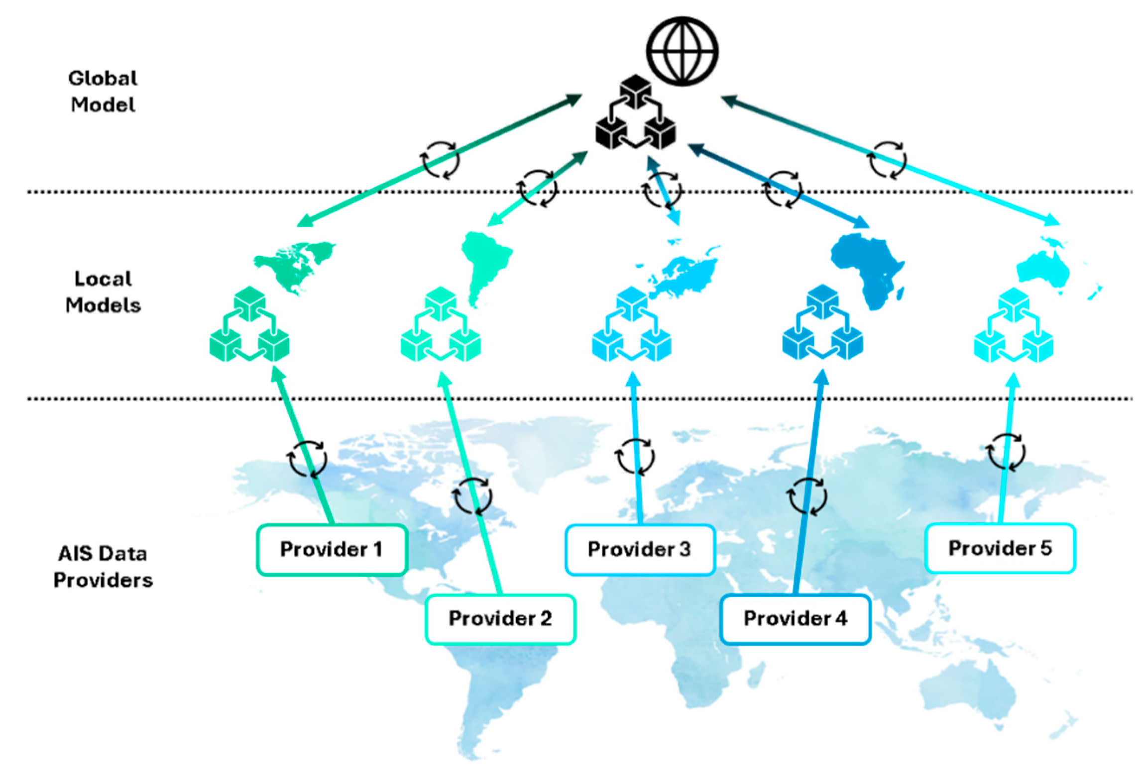
The proposed solution implements a lifelong learning cycle. Figure 1 shows five hypothetical AIS data providers, each continuously supplying AIS data from different regions. In the first cycle, each provider uses recent data (e.g., from the previous month) to calculate vessel traffic densities and train local prediction models. Local model weights are sent to a central server and federated into a global model. The resulting global model weights are then back-propagated to update local models. In subsequent cycles, providers continue updating local models with new data and density calculations, sending updated weights to the central server, which refines the global model and redistributes the new federated weights. The integration of EMODNet’s VTD method, CNN-based local training, and model federation via FL represents a novel and disruptive approach in the current literature.
This back-propagation approach keeps all local models synchronized with the global model, allowing for the selection of the most accurate one. The choice between local or global model weights is based on accuracy metrics: if a local model achieves better accuracy than the global model, its weights are retained; otherwise, the global model’s weights are adopted for predicting local vessel traffic densities. This selection scheme also applies to global model versions. If a newer version outperforms its best predecessor in accuracy, its weights are backpropagated to the providers. If the predecessor performs better, due to overfitting in the newer model, for instance, then its weights are used instead. This ensures that providers always have access to the most accurate density predictions.
Figure 1.
Lifelong Federated Learning cycle for the proposed solution.
Section 1 outlined the research context and key challenges addressed and introduced the proposed solution, along with a review of relevant state-of-the-art. Section 2 details the materials and methods, including AIS datasets, development steps, and methods for VTD calculation, local model training, and global model federation. Section 3 presents the evaluation results of model training and federation. Finally, Section 4 discusses the outcomes, explores future research directions, and concludes the study.
2. Materials and Methods
This section outlines the proposed solution’s processes, from data collection and pre-processing to VTD calculation using EMODNet’s method, density prediction model training, and global model federation via FL.
2.1. Selected Datasets, Data Collection and Pre-Processing
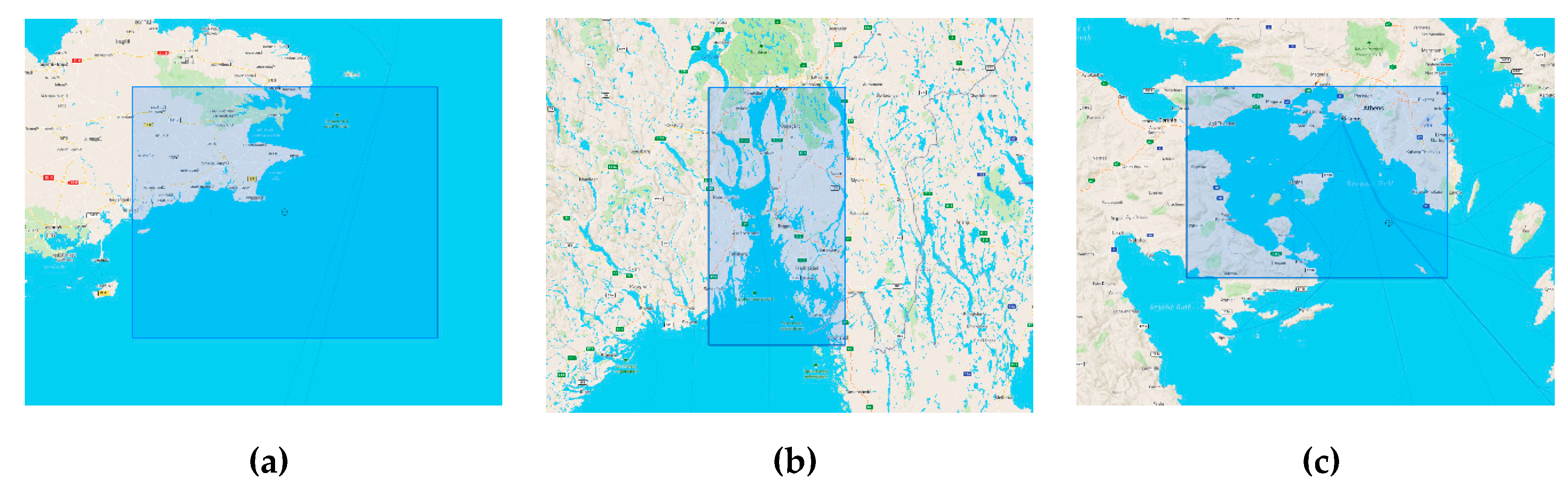
Since public real-time AIS datasets are not easy to find, the selected approach is based on historical data, which were divided into monthly batches. Three datasets were selected: the Brest dataset (Brest coast and port area, France, Atlantic Ocean — Figure 2a) [29], the Kystverket dataset (Oslo Fjord area, Norway, Baltic Sea — Figure 2b) [30] and the Piraeus dataset (Athens coast and port area, Greece, Mediterranean Sea — Figure 2c) [31].
Figure 2.
Bounding boxes defining spatial boundaries for the three datasets: (a) Brest; (b) Kystverket; and (c) Piraeus.
Figure 2.
Bounding boxes defining spatial boundaries for the three datasets: (a) Brest; (b) Kystverket; and (c) Piraeus.
Although some datasets span multiple years, only one year was used from each. For Brest, only six months, from October 2015 to March 2016, were used. For Piraeus and Kystverket, the whole year of 2019 was selected. These datasets were chosen either because they are publicly available or fall within the scope of the European Commission-funded HORIZON 2020 VesselAI project [32].
Each dataset originates from different sources and collection methods: Brest and Piraeus were downloaded, while Kystverket was obtained via Application Programming Interface (API). Although all were retrieved in Comma-Separated Values (CSV) format, each has a unique schema and set of fields.
A data harmonisation step was applied to unify all datasets into a common schema, depicted in Table 1, facilitating subsequent data processing tasks.

Table 1.
Common database reference schema for the three AIS datasets.
| Field Name | Data Type | Description |
|---|---|---|
| OID | Object ID | Unique identifier of the AIS message |
| MMSI | Long Integer | Vessel MMSI identifier |
| Lon | Double | WGS84 longitude value |
| Lat | Double | WGS84 latitude value |
| DateTime | Timestamp | Timestamp object of the AIS message |
| Sog | Integer | Speed over ground value in knots |
| Cog | Integer | Course over ground value in degrees |
| Heading | Integer | Heading value in degrees |
In Table 1, “OID” is the unique identifier of each AIS message, “MMSI” (Maritime Mobile Service Identity) identifies individual vessels, “Lat” and “Lon represent latitude and longitude in the WGS84 reference system, “DateTime” is the AIS message’s UNIX timestamp, “Sog” is the vessel’s speed over ground (knots) and “Cog” and “Heading” are, respectively, the vessel’s course over ground and heading (degrees). After harmonisation, all datasets underwent a data cleaning process based on the following steps: (i) Removal of duplicate messages, (ii) removal of irrelevant message types, as described in [15], (iii) removal of missing or incomplete data, and (iv) removal of messages with wrong or anomalous values, based on [15].
2.2. Vessel Traffic Density Calculation
The VTD calculation was based on EMODNet’s Vessel Density Map method, which will be presented in the following subsections.
2.2.1. Defining the Area of Interest
The Area of Interest (AoI) defines the spatial boundaries of each dataset represented in Figure 2. Each AoI is a four-sided polygon aligned with Earth’s curvature, with edges determined by the minimum and maximum latitudes and longitudes of the respective dataset. Table 2 provides key details about each dataset and its AoI, including the total spatial area in squared kilometres, the total number of AIS messages, the average monthly message count, and the number of months covered.
Table 2.
Dataset facts and figures.
| Dataset | AoI Total Area (Km2) | Total Number of Messages | Monthly Average Number of Messages | Number of Months |
|---|---|---|---|---|
| Brest | 25.456 | 16.356.036 | 2.726.006 | 6 |
| Piraeus | 9.504 | 92.534.303 | 8.004.870 | 12 |
| Kystverket | 15.776 | 53.065.140 | 4.421.921 | 12 |
2.2.2. Creating a Grid
Grids are geographic bounding boxes divided into uniform square cells, defined using GIS methods. Various cell sizes were tested, as each serves different analytical purposes and presents trade-offs for VTD calculation. Smaller grid cells offer more detailed density insights but can degrade calculation performance over large AoIs and increase sparsity in the final dataset, posing challenges for training prediction models (the sparsity challenge is discussed in later subsections). Conversely, larger cells improve performance in both density calculation and model training but reduce spatial detail, potentially offering an overly general view of vessel traffic.
Grid cell size selection is also influenced by datasets’ temporal characteristics, particularly span and granularity. For shorter spans, such as one hour or one day, larger cell sizes are recommended to avoid overly sparse density values due to fewer AIS messages, as opposed to a monthly span, for instance. The recommended span also depends on the actual temporal granularity of the density calculation, i.e., the time interval considered to calculate a specific cell’s density. Lower granularity (e.g., vessels passing through a cell over one week) yields denser values, while higher granularity (e.g., one-minute intervals) increases sparsity, making prediction more challenging.
Multiple tests were conducted using different cell sizes, time spans, and granularities. Although each AoI varies in size, a uniform grid cell size, temporal granularity, and time span across all datasets is preferred. A balanced configuration, minimizing data sparsity while maintaining spatial detail, was achieved using a one-month span, one-hour granularity and four-by-four-kilometre grid cells. To define grid cells in kilometres, the distance-based ETRS89-LAEA Europe (EPSG:3035) coordinate system was used. PostGIS transformation functions converted AIS coordinates from the original angle-based WGS84 system (EPSG:4326) to ETRS89-LAEA.
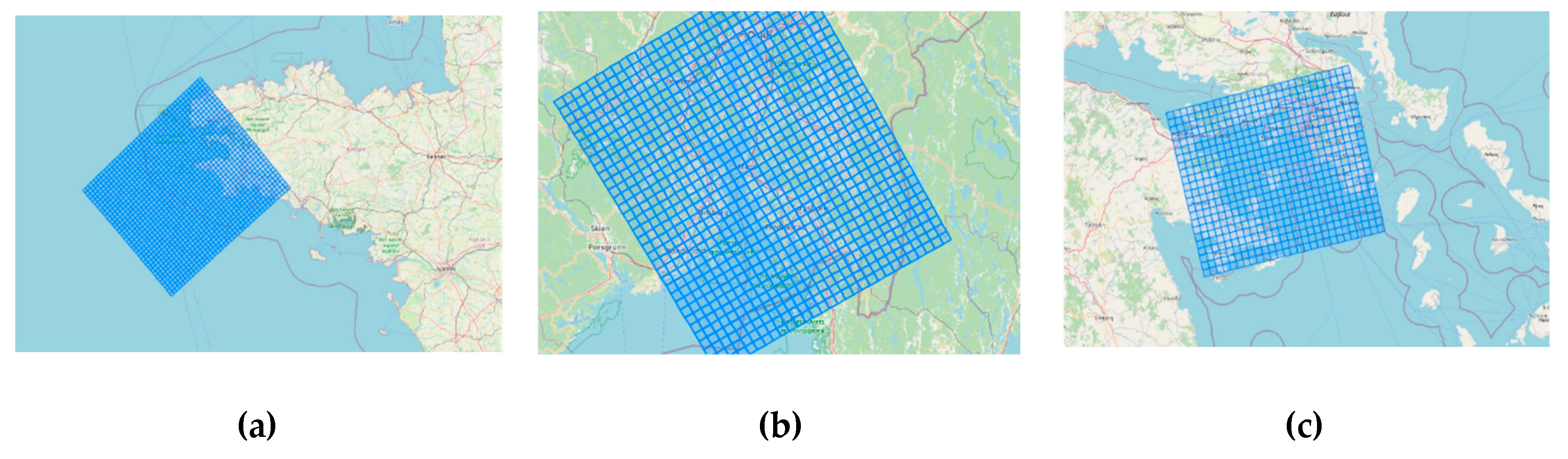
PostGIS functions were used to define four-by-four-kilometre grid cells covering the AoIs presented in Figure 2 and to transform distance-based coordinates back to WGS84. Grid cell data was stored in a new database table, the Grid table, which includes a cell identifier (“CellID”), minimum and maximum latitudes and longitudes, and a geometry object (“Shape”) representing the cell’s spatial polygon. Figure 3 depicts the resulting grids: (a) Brest, (b) Kystverket, and (c) Piraeus.
Figure 3.
Spatial grids for Brest (a), Kistverket (b) and Piraeus (c) datasets.
2.2.3. Creating Points and Lines
The next step involved creating tables for points and lines. Each point represents positional and spatial data from each AIS message, while each line connects two temporally consecutive spatial points from the same vessel, forming a straight-line segment. The Point table was generated by processing AIS messages using a custom Python script, with its structure detailed in Table 3.
Table 3.
Point database table reference.
| Field Name | Data Type | Description |
|---|---|---|
| OID | Object ID | Unique identifier of the point |
| Shape | Geometry | POINT geometry object |
| MMSI | Long Integer | Vessel MMSI identifier |
| Lon | Double | WGS84 longitude |
| Lat | Double | WGS84 latitude |
| DateTime | Date | DATETIME object of the point |
| X1 | Double | LAEA longitude value |
| Y1 | Double | LAEA latitude value |
In Table 3, “OID” is the unique identifier for each point, “Shape” is a PostGIS geometry object generated from the vessel’s WGS84 coordinate, “Lat” and “Lon” represent the point’s latitude and longitude, respectively. “MMSI” is the vessel’s unique identifier, “DateTime” represents the AIS message’s timestamp, “X1” and “Y1” are horizontal and vertical coordinates in the LAEA reference system, used to calculate distances in metres between consecutive points.
Once AIS data is processed and stored as points, the Point table is sorted by “MMSI” and “DateTime.” A Python script processes the sorted data to generate Line data. For every two consecutive Point records, the script creates and stores a Line record, structured as depicted in Table 4.
Table 4.
Line database table reference.
| Field Name | Data Type | Description |
|---|---|---|
| OID | Object ID | Unique identifier of the line |
| Shape | Geometry | LINE geometry object |
| MMSI | Long Integer | Vessel MMSI identifier |
| Lon1 | Double | WGS84 longitude of point 1 |
| Lat1 | Double | WGS84 latitude of point 1 |
| Lon2 | Double | WGS84 longitude of point 2 |
| Lat2 | Double | WGS84 latitude of point 2 |
| LineTime | Double | Time difference (seconds) between point 1 DateTime and point 2 DateTime |
| ShapeLength | Double | Line length (meters) between point 1 and point 2 |
| DateTime1 | Date | DATETIME object of point 1 |
In Table 4, “OID” is the unique identifier for each line, “Shape” is the geometry generated by PostGIS. “MMSI” is the vessel’s unique identifier. “X1” and “Y1” are the latitude and longitude of the origin point, while “X2” and “Y2” are those of the destination point, in WGS84. “LineTime” is the time in seconds the vessel takes to travel between the two points, based on the difference between their “DateTime” values. “ShapeLength” is the line's length in metres, and “Datetime1” is the origin point’s timestamp.
2.2.4. Calculating Density
The EMODNet grid-based density calculation method [9] computes a density value for each grid cell using the Line data described in the previous subsection. As noted earlier, the first step involves generating a grid cell table. Each row includes a “CellID,” a unique index ranging from 0 to the total number of cells minus one, and a “Shape” parameter, representing the geographic square polygon of the cell based on its Earth surface position. The EMODNet’s density calculation method defines a cell’s density, ρ, as a measure of the total time spent in the cell for all vessels that crossed that cell and is calculated via Equation (1).
ρ = ( length in cell / total length ) * total time
A new database table, Density, was created to store grid cell density values calculated using Equation (1). It includes “CellID,” corresponding to the unique identifier from the Grid table; “Year,” “Month,” “Day,” and “Hour,” indicating the time associated with each density value; and “Density,” which stores the value ρ for the respective cell and time interval defined by the temporal granularity. A stored procedure was developed in PostgreSQL to perform the following PostGIS-supported tasks: (i) sort lines by MMSI, hour, day, month, and year; (ii) intersect lines from the Line table with Grid cells using the “st_intersection” function; (iii) define a variable SEGLENGTH and compute segment length using “st_length”; (iv) define SEGTIME and calculate segment time using Equation (2); (v) sum segment times within each cell to derive ρ; and (vi) store the results in the Density table.
SEGTIME = ( SEGLENGTH / ShapeLength ) * LineTime
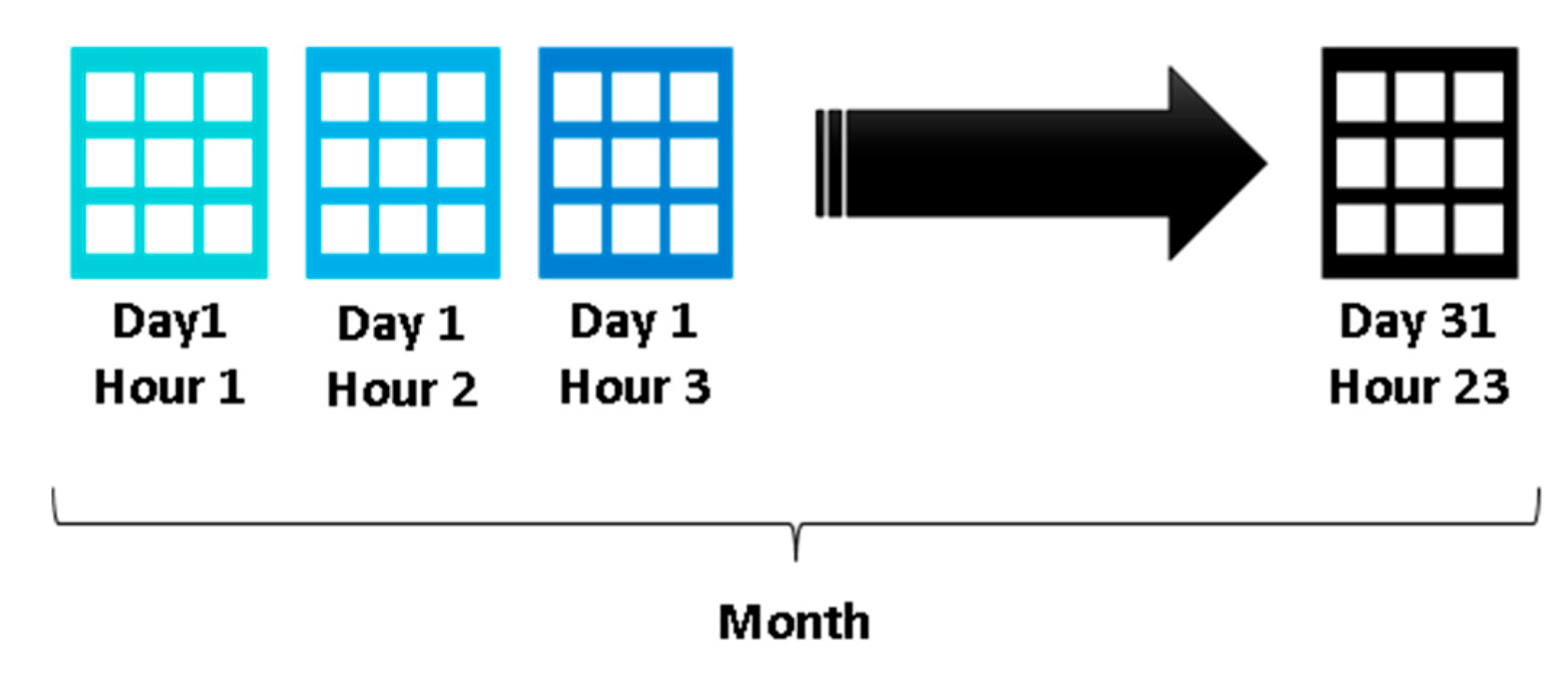
The resulting Density table represents a monthly aggregation of hourly density matrices, aligned with the temporal span and granularity defined during grid definition. Each matrix’s dimensions match the number of horizontal and vertical cells in the AoI grid. Figure 4 illustrates this structure. For a 31-day month like March, there are 744 matrices. Matrix size varies by dataset (e.g., Brest has a 43×37 grid, Piraeus 23×27, and Kystverket 29×34).
Figure 4.
Monthly aggregation of hourly density matrices.
A key characteristic of these matrices is their sparsity, i.e., most cell density values are zero. This results from two factors: vessel traffic typically follows specific routes or “sea highways,” leaving most water-based cells with zero or near-zero density, except those along these routes; and squared grids may include land-based cells, which always have zero density since AIS data is not recorded on land.
A final note concerns hourly matrices composed entirely of zero-density values, typically due to missing or cleaned AIS messages for the entire hour. For instance, in March 2019, the Piraeus dataset yielded only 739 matrices instead of the expected 744, indicating 5 hours with no data available. Given that it is highly unlikely for the Piraeus port area to have zero traffic during any hour, these zero-density matrices are considered erroneous and were excluded prior to VTD prediction model training.
2.3. Training Local Vessel Traffic Density Prediction Models
Based on current state-of-the-art, and to the best of the authors’ knowledge, few studies focus on predicting VTD using Federated, Lifelong Learning or DL methods. Consequently, it is difficult to rely on prior problem definitions. The authors examined the Density table’s characteristics to identify parallels with advanced studies that could provide insights or inspiration. As shown in Figure 4, each matrix represents the hourly cumulative density for a specific day and location, with each cell corresponding to a spatial position. Density patterns in each cell are primarily influenced by two factors: its own activity in the preceding hours and the activity in surrounding cells during the same period. From another perspective, each hourly density matrix can be seen as a grayscale image representing vessel traffic in the AoI at a specific time. In this interpretation, each cell acts as a pixel with a single hue, the density value, unlike colour images, which have multiple hue values (e.g., Red, Green, Blue).
In this context, the task resembles an image processing-based next-frame prediction problem, developing a model that transforms sparse input density matrices into future states of the same shape, as a matrix-to-matrix transformation. This model aims to predict the future state of the density grid while maintaining the same matrix shape. Each cell’s density depends on its previous state, giving the data a time-series of images nature (Figure 5). Leveraging convolutional layers for spatial feature extraction and temporal pattern learning is a promising approach.
CNN are designed to process grid-like data structures, such as images or matrices. As noted earlier, an image is a grid of pixels, each holding brightness and colour values. For grayscale images, each pixel contains a single value, mirroring matrix structures. The sparse matrices generated by EMODNet’s density calculation can be interpreted as grayscale images in a time series with hourly granularity, where each cell acts as a pixel representing vessel density.
Figure 5.
VTD prediction problem definition.

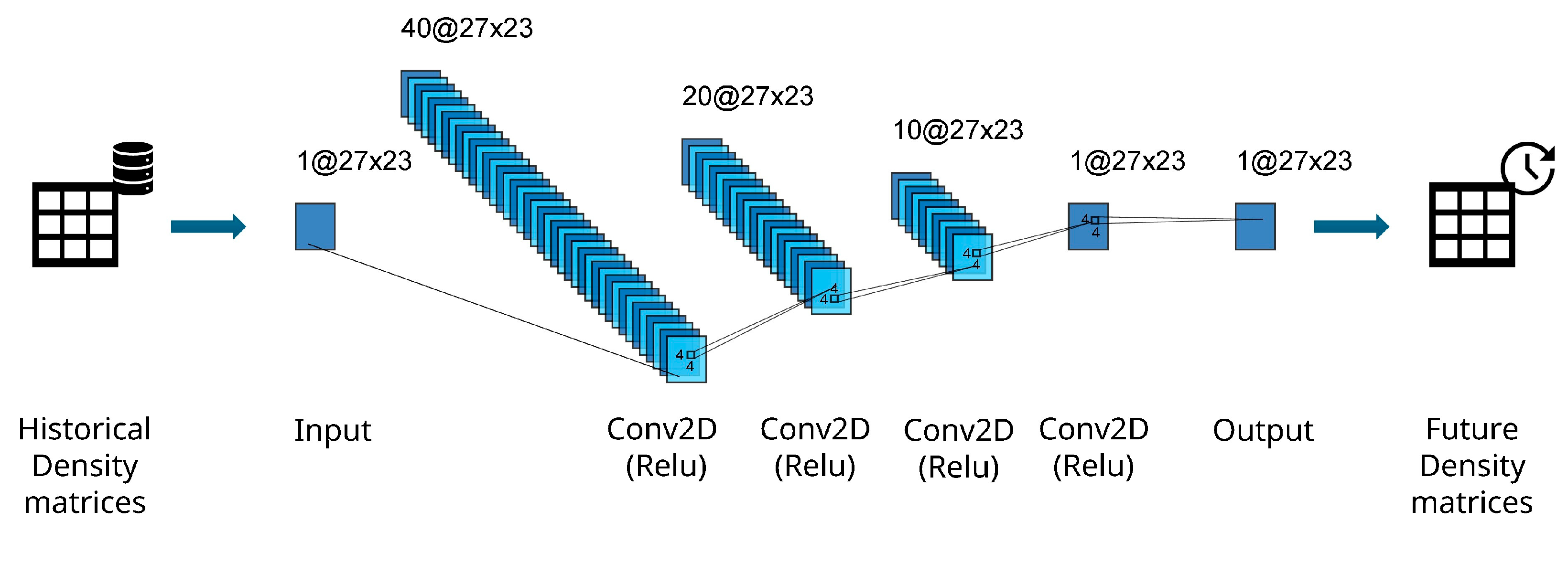
This approach was selected after a thorough evaluation of methods suited to the problem’s characteristics defined in Figure 5, such as fixed matrix size and sparsity. The architecture, number of convolutional layers, kernels per layer, and other hyperparameters were determined through extensive experimentation with different CNN configurations. Hence, the authors deployed the architecture presented in Figure 6, with four Conv2D convolutional layers’ shapes, comprising the number of horizontal cells and the number of vertical cells of the density matrices generated for the Brest dataset, along with each layer’s number of filters (respectively, 40, 20, 10 and 1 filter). All convolutional layers use a 4x4 kernel and ReLu as the activation function, with the same padding across layers to keep the original spatial structure of the input matrices.
The choice for such a simple architecture was mainly due to the limited number of matrices in the prepared datasets (700 ~800) and to the need of efficiency of model training tasks in local on-premises machines. Mean Squared Error (MSE) was the model's loss function applied and ADAM the hyperparameter optimiser technique, with a learning rate of 1x10⁻⁴. 3-fold cross-validation for time-series data was employed to optimise the hyperparameters. The CNN architecture was developed using Keras [35].
This model performs a series of convolutional transformations on a grayscale 2D input to produce a single-channel output, with the intention of performing image-to-image regression over heatmap-like matrices.
Figure 6.
CNN architecture for the Brest dataset.
2.4. Global Vessel Traffic Density Prediction Model Federation
Federated Learning (FL) is a decentralized machine learning approach that enables model training across multiple devices without sharing raw data, preserving data privacy and supporting localized training without requiring high-performance hardware. The process begins by training local models on each data provider’s on-premises or cloud servers using local datasets. Instead of sharing raw data, the local models’ weights, capturing the behaviour of local data, are sent to a central server for aggregation using FL techniques.
This aggregation produces a global federated model that reflects the implicit behaviour of all local models. The global model’s weights are then shared with local data providers and evaluated against their local weights for prediction accuracy and error handling. Providers can choose to adopt global weights or retain their local weights for future predictions and model updates. This iterative process continually refines the global model, incorporating insights from diverse datasets.
This study adopts a horizontal FL approach to structure the server–client model and manage data sharing. In horizontal FL, data is distributed across multiple devices or servers, each holding different records but with the same feature set. A shared model is collaboratively trained without exchanging raw data. Each device trains locally and sends only model updates to a central server for aggregation. This approach is well-suited for privacy-sensitive contexts, as data remains on local devices while still enabling collective learning. It is ideal for horizontally partitioned data, where each device has distinct examples but identical features [36].
Several FL libraries were reviewed and tested to identify the best fit for the proposed solution [37]. Flower [38], an open-source FL framework, proved most suitable due to its flexible, modular architecture that supports integration with major ML frameworks like TensorFlow and PyTorch. Its ability to handle slow or delayed clients and reduce model update sizes is particularly advantageous. Additional strengths include cross-platform compatibility, adaptability to various devices, and scalability to millions of clients. Figure 7 depicts the Flower-based FL client-server structure. During scheduled communication, not all clients may be available, due to being offline or lacking data or resources, thus the global model is updated using only the weights from available clients.
Figure 7.
Flower FL server-client architecture [38].
Figure 7.
Flower FL server-client architecture [38].
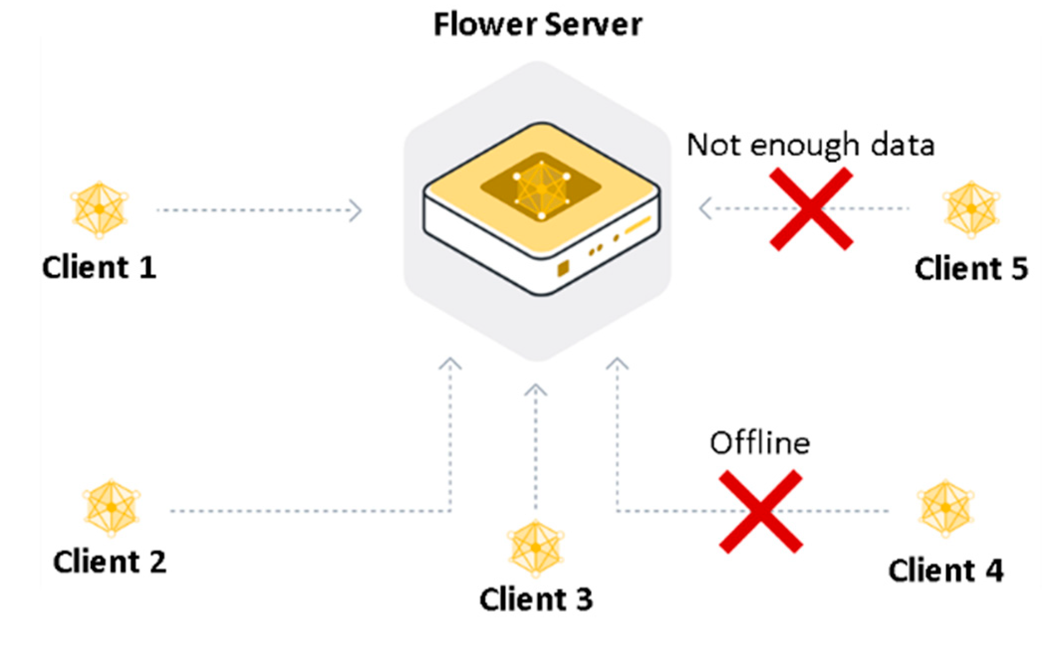
All clients in the pool can access the server’s aggregated parameters at any time. In the architecture shown in Figure 7, a cyclical process unfolds (with a predefined or infinite number of repetitions n, as in lifelong learning): (i) train/update local models offline; (ii) select available clients; (iii) transmit local weight representations to the server; (iv) aggregate weights on the server using the “FedAvg” function; (v) compare new global weights with previous best to select those for dissemination; (vi) distribute global weights to all available clients; (vii) compare global and local weights to choose the best for updating; (viii) repeat from step 1 for the next round. The Flower server was deployed on a dedicated IP address accessible to clients, with three specialized clients handling the Brest, Piraeus, and Kystverket datasets, each responsible for training and updating its CNN model. While preprocessing steps and input structures may vary slightly across datasets, they share a common network architecture. Each dataset was split into three segments: the first two used for training, and the third for predicting the future grid.
3. Results
This section presents an evaluation of the results from both local and global model training. As previously noted, density matrices are inherently sparse due to vessel routes and nearby land areas lacking vessel presence. To address this, Sparse Mean Square Error (Sparse MSE) [39] was used as the primary accuracy metric, focusing on prediction precision for non-zero cells, providing a more meaningful evaluation of model performance in sparse contexts. First, to demonstrate the quality of the CNN model depicted in Figure 6, the authors performed a comparison between the chosen model and three other state-of-the-art approaches available in the literature, as presented in Table 5. The comparison was made by training all models with a month worth of data extracted from the Piraeus dataset. The selected month was the one in which the 4-layer CNN mode of Figure 7 presented the best result.
Table 5.
Prediction accuracy comparison between the 4-layer CNN model and three other state-of-the-art models. The metric used is Sparse MSE. The ‘*’ means that, although the model presents the best SparseMSE result, it has also really high computing infrastructure requirements.
Table 5.
Prediction accuracy comparison between the 4-layer CNN model and three other state-of-the-art models. The metric used is Sparse MSE. The ‘*’ means that, although the model presents the best SparseMSE result, it has also really high computing infrastructure requirements.
| Model | Reference | Sparse MSE (best) |
|---|---|---|
| 4-layer CNN | Figure 7 | 0.0028 |
| CNN-LSTM Autoencoder | [40] | 0.00065* |
| Keras CNN-LSTM Autoencoder | [41] | 0.0323 |
| Pyramid CNN Autoencoder | [42] | 0.0079 |
The 4-layer CNN model proposed in this work performs better than two of the state-of-the-art models, in terms of Sparse MSE. The best-performing model is the one proposed in [40] but it presents severe limitations in terms of model training performance, since it is a 11-layer CNN-LSTM with transformation steps between layers. The proposed 4-layer CNN outperforms most of the models in terms of accuracy and presents a good balance in terms of computing performance and prediction accuracy.
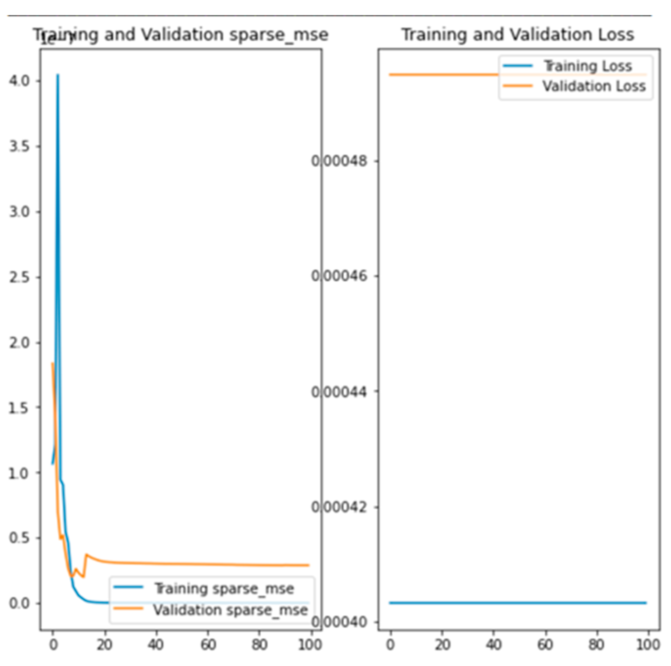
To determine convergence, each local CNN model was trained for 100 epochs. Figure 8 depicts the Piraeus model’s training results over 100 epochs, with the horizontal axis representing epoch count and the vertical axis showing training/validation loss (right) and Sparse MSE (left). The global federated weights were sent back to local clients, where they were validated and compared with local weights using Sparse MSE. Table 6 presents the validation results for both local and global Sparse MSE across the three datasets. In the first iteration, the local models for Piraeus and Kystverket outperformed the global model, though the differences were small. Conversely, the global model performed better on the Brest dataset.
Table 6.
Sparse MSE validation results for local and global models for the three datasets (first month of data). Best result for each dataset is marked in bold.
Table 6.
Sparse MSE validation results for local and global models for the three datasets (first month of data). Best result for each dataset is marked in bold.
| Dataset | Local Sparse MSE (first month) | Global Sparse MSE (first month) |
|---|---|---|
| Brest | 0.0312 | 0.0294 |
| Piraeus | 0.0030 | 0.0048 |
| Kystverket | 0.0023 | 0.0030 |
The discrepancy in results for the Brest dataset, along with higher error values for both local and global models, stems from its characteristics. The Brest AoI is significantly larger—nearly four times Piraeus and three times Kystverket—yet it contains only half the monthly AIS records of Kystverket and a quarter of Piraeus (see Table 2). This results in much sparser density matrices, making accurate VTD prediction more difficult. This situation mirrors the “not enough data” challenge in FL, where clients with limited data benefit from aggregated global weights. This aligns with the results in Table 6, in which the global model outperforms the local model on Brest data, a trend that becomes more evident in subsequent lifelong learning iterations.
Figure 8.
MSE loss (right) and Sparse MSE (left) values for training and validation of the Piraeus local model.
Figure 8.
MSE loss (right) and Sparse MSE (left) values for training and validation of the Piraeus local model.
After the initial iteration, each subsequent round updated local models with one month of data. Local weights were sent to the server to update the global model, whose new weights were then propagated back to clients and compared against updated local weights using Sparse MSE. The better-performing weights, local or global, were retained for the next iteration. From the second month onward, global weights generally outperformed local ones, with only minor exceptions. This is well expressed in Table 7, which depicts the validation Sparse MSE results for both local and global models during the best-performing month overall.
Table 7.
Sparse MSE validation results for local and global models for the three datasets (best month). Best result for each dataset is marked in bold.
Table 7.
Sparse MSE validation results for local and global models for the three datasets (best month). Best result for each dataset is marked in bold.
| Dataset | Local Sparse MSE (best) | Global Sparse MSE (best) |
|---|---|---|
| Brest | 0.0276 | 0.0072 |
| Piraeus | 0.0028 | 0.0013 |
| Kystverket | 0.0018 | 0.0016 |
The results indicate that, overall, the global model improves through iterations and eventually outperforms local models in predicting hourly VTD across all AoIs. Still, aside from the Brest case, both local and global models yield low and closely aligned Sparse MSE values, demonstrating strong predictive performance. However, ongoing testing with more data over multiple years is needed to validate these findings, particularly to assess seasonality effects and potential overfitting in both local and global models.
Figure 9 presents the VTD prediction grids for a sample hour in the month of March (i.e., third iteration) for all three AoIs: the left column represents the Brest AoI; the centre column represents the Kystverket AoI; and the right column represents the Piraeus AoI.
Figure 9.
Sample predictions from local and global models for the best-performing month (based on Sparse MSE): ground truth (top), local model prediction (middle), and federated model prediction (bottom) for Kystverket (left), Piraeus (centre), and Brest (right) datasets. The figures use a red-to-white colour gradient, with darker reds denoting lower VTD and lighter shades indicating higher VTD values.
Figure 9.
Sample predictions from local and global models for the best-performing month (based on Sparse MSE): ground truth (top), local model prediction (middle), and federated model prediction (bottom) for Kystverket (left), Piraeus (centre), and Brest (right) datasets. The figures use a red-to-white colour gradient, with darker reds denoting lower VTD and lighter shades indicating higher VTD values.
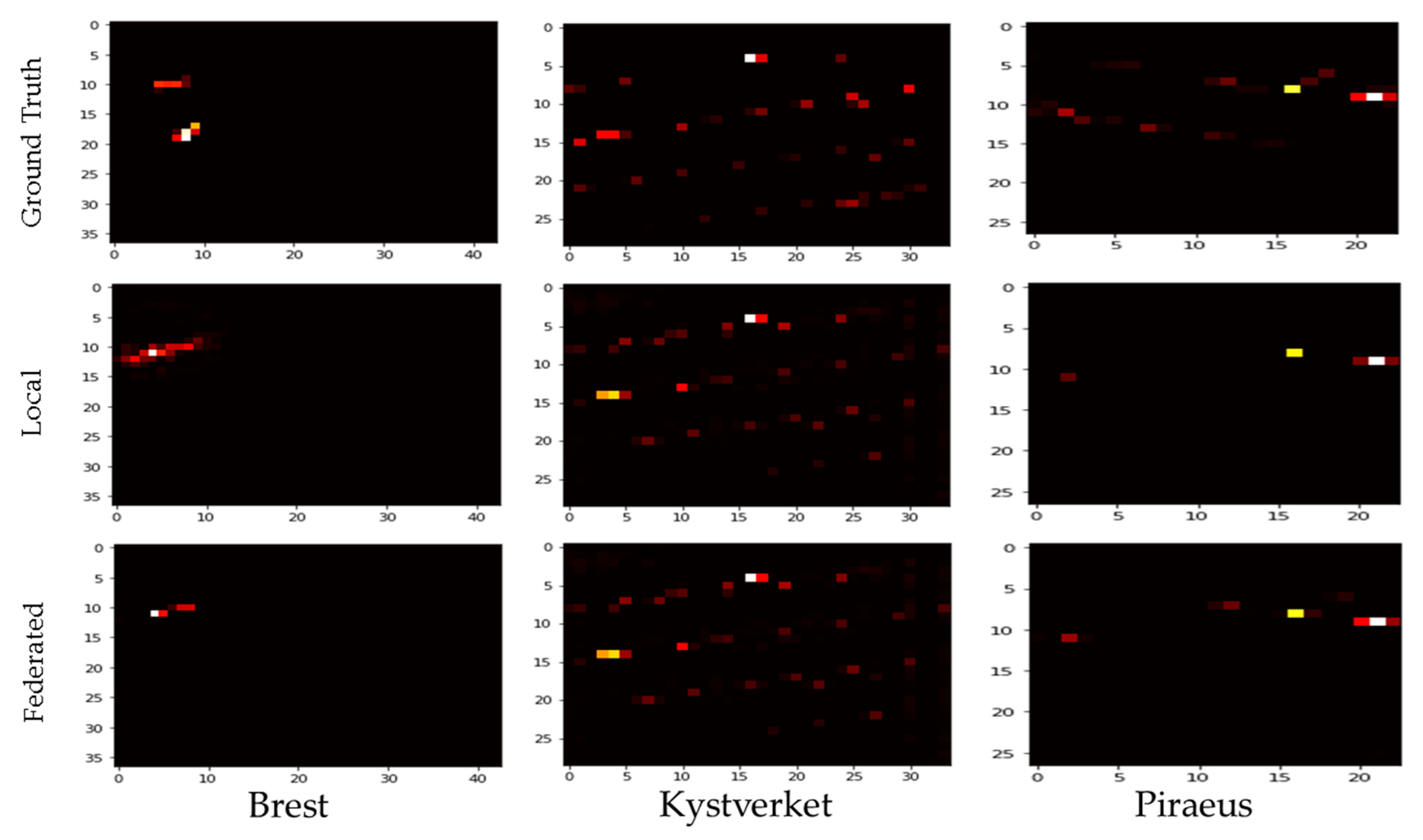
The top row shows the ground truth for the sample hour, while the middle and bottom rows display the VTD predictions from the local and global models, respectively. The outputs align with the results in Table 7: (i) predictions for the Brest AoI are generally less accurate, though the federated model outperforms the local one; (ii) for both Kystverket and Piraeus, local and global models provide strong predictions, with the global model performing slightly better. As part of the European Commission-funded VesselAI project, a visualization dashboard was developed using Apache Superset [43] to analyse and evaluate both models’ results against ground truth data for specific periods (e.g., day, hour).
4. Discussion and Conclusions
This work presents a novel, privacy-preserving, and performance-aware framework for VTD prediction using AIS data, integrating EMODNet’s standardised VTD calculation with CNN- and FL-based methods. The approach tackles two key maritime data science challenges: protecting proprietary AIS information and managing the computational and storage demands of AIS Big Data. A major strength is its FL-based distributed architecture, which decentralises model training across local hardware, preserving data privacy and reducing reliance on centralised systems. By training models near the data source and sharing only model weights, the approach cuts communication overhead and infrastructure needs, offering a scalable, cost-effective alternative to traditional centralised methods.
Empirical results show that the federated global model generally outperforms local models in data-sparse regions while maintaining strong accuracy across all validation cases. This highlights the approach’s effectiveness and adaptability across varying scenarios and data profiles, delivering acceptable accuracy while preserving data privacy. A key challenge, however, lies in the high sparsity of density matrices. Neural networks are typically optimised for rectangular inputs, making it difficult to exclude land regions or isolate specific maritime routes. Attempts to reduce the AoI and input size had limited success. Future work should investigate methods for processing non-rectangular or irregular spatial inputs to better capture actual vessel traffic areas.
Another major challenge is the hardware-intensive and time-consuming nature of data preparation and model training. Table 8 depicts the monthly average data volumes collected or generated during these tasks. Pre-density processing, such as grid cell mapping and calculating SEGLENGTH, SEGTIME, and ρ, produces significant data, often in the tens or hundreds of gigabytes. Overcoming these bottlenecks and integrating more data over time within a lifelong learning framework could greatly improve the global model’s predictive capability. Still, these challenges reinforce the approach’s core advantage: distributing data preparation and training across local clients while sharing only model weights, rather than centralizing these tasks and transmitting raw data, offers clear scalability and efficiency benefits.
Table 8.
Monthly average data volumes (collected or generated) for different stages of the data processing and model training tasks, for the three AoIs.
Table 8.
Monthly average data volumes (collected or generated) for different stages of the data processing and model training tasks, for the three AoIs.
| Data Type | Brest | Kystverket | Piraeus |
|---|---|---|---|
| AIS Records | ~108.79 MB | ~340.48 MB | ~304.48 MB |
| Pre-density | ~49.21 GB | ~455.69 GB | ~87.21 GB |
| Density Matrices | ~39.59 MB | ~36.46 MB | ~15.7 MB |
| Model Weights | ~2MB | ~2MB | ~2MB |
The resource-intensive processes are distributed, allowing clients to require fewer hardware resources for local data processing and model training. Additionally, no explicit data is shared, meeting clients’ privacy requirements. A third benefit arises from both goals: the proposed approach significantly reduces data communication needs, as only model weights, not raw data, are exchanged between clients and server. As seen in Table 8, model weights offer the most communication-efficient option due to their smaller data volume, enabling faster transmissions within the FL client-server architecture.
Implementing a true lifelong learning strategy on the server side is a crucial next step for developing a more adaptable and competitive global model. This involves continuously aggregating client updates, even when model architectures differ, to produce a refined, representative global model. As the current approach used only one year of data, extending the deployment period may introduce challenges such as detecting seasonality patterns or managing overfitting. Additionally, the present method updates local models monthly using hourly-resolution data. Future work should explore lifelong learning-related challenges, along with alternative update frequencies and temporal granularities, to enhance both performance and computational efficiency.
Finally, alternative methods and technologies should be explored. As models accumulate knowledge, more advanced architectures like LSTM-CNN hybrids or Sparse GANs become viable. LSTMs are effective for capturing temporal dependencies in time-series data, while Sparse GANs are promising for modelling sparse datasets. Though these models could reduce Sparse MSE and enhance prediction quality, they also increase computational demands, especially on the client side. Additionally, for efficient model versioning and continuous learning, tools like MLFlow offer a robust platform for storing, tracking, and managing both local and global models, as will be validated during the AI-DAPT research project [44]. This enables clients to retain and compare historical model versions across types and training periods. The proposed solution provides a solid foundation for real-world maritime traffic forecasting, delivering actionable insights for safety, environmental protection, and port logistics. Overall, this study effectively demonstrates how federated, distributed AI can enable powerful predictive capabilities in privacy-sensitive, data-intensive domains like global maritime operations.
Author Contributions
Conceptualisation, Amin Khodamoradi, Paulo Figueiras, Luis Lourenço, André Grilo, Bruno Rêga; Data curation, Amin Khodamoradi, Luis Lourenço, André Grilo, Bruno Rêga; Formal analysis, Methodology, Investigation, Software, Validation & Visualisation, Amin Khodamoradi, Paulo Figueiras, Luis Lourenço, André Grilo, Bruno Rêga; Funding acquisition, Resources & Project administration, Paulo Figueiras, Carlos Agostinho, Ruben Costa, Ricardo Jardim-Gonçalves; Writing – original draft, Paulo Figueiras, Amin Khodamoradi; Writing - review & editing, Paulo Figueiras, Ruben Costa, Carlos Agostinho, Ricardo Jardim-Gonçalves.
Funding
This research was funded by the European Commission, under the scope of the VesselAI research project [32], Grant agreement ID: 957237, and the AI-DAPT research project [44], Grant agreement ID: 101135826.
Data Availability Statement
Conflicts of Interest
The authors declare no conflicts of interest. The funders had no role in the design of the study; in the collection, analyses, or interpretation of data; in the writing of the manuscript; or in the decision to publish the results.
Abbreviations
The following abbreviations are used in this manuscript:
| AI | Artificial Intelligence |
| AIS | Automatic Identification System |
| AoI | Area of Interest |
| API | Application Programming Interface |
| CNN | Convolutional Neural Networks |
| CSV | Comma Separated Values |
| DL | Deep Learning |
| EMODNet | European Maritime Observation and Data Network |
| EPSG | European Petroleum Survey Group |
| ETRS89 | European Terrestrial Reference System 1989 |
| FL | Federated Learning |
| GANs | Generative Adversarial Networks |
| GB | Gigabytes |
| GIS | Geographic Information Systems |
| IoT | Internet of Things |
| IP | Internet Protocol |
| LAEA | Lambert azimuthal equal-area projection |
| LSTM | Long Short-Term Memory |
| MB | Megabytes |
| ML | Machine Learning |
| MMSI | Maritime Mobile Service Identity |
| MSE | Mean Squared Error |
| UNCTAD | United Nations Conference on Trade and Development |
| VTD | Vessel Traffic Density |
| WGS84 | World Geodetic System 1984 |
| XGBoost | eXtreme Gradient Boosting |
References
- Lavery, B. A Short History of Seafaring, London, UK: Dorling Kindersley Ltd., 2022.
- United Nations Conference on Trade and Development, “Review of Maritime Transport 2022: Navigating Stormy Waters,” United Nations, Geneva, Switzerland, 2022.
- European Maritime Safety Agency , “Annual Overview of Marine Casualties and Incidents 2024,” European Union, Lisbon, Portugal, 2024.
- Transportation Safety Board of Canada, “Statistical Summary: Marine Transportation Occurrences in 2020,” Government of Canada, Gatineau, Quebec, Canada, 2020.
- Munim; Z.H.; Dushenko; M.; Jimenez; V.J.; Shakil; M.H.; Imset, “Big Data and Artificial Intelligence in the Maritime Industry: a Bibliometric Review and Future Research Directions,” Maritime Policy & Management, vol. 47, no. 5, pp. 577-597, 2020. [CrossRef]
- Tijan, E.; Jović, M.; Aksentijević, S.; Pucihar, A. , “Digital Tansformation in the Mritime Tansport Sctor,” Technological Forecasting and Social Change, vol. 170, 2021. [CrossRef]
- Emmens, T.; Amrit, C.; Abdi, A.; Ghosh, M. , “The Promises and Perils of Automatic Identification System Data,” Expert Systems with Applications, vol. 178, 2021. [CrossRef]
- Sun, J.; Yi, Z.; Zhuang, Z.; Jiang, S. , “Securing Automatic Identification System Communications Using Physical-Layer Key Generation Protocol,” Journal of Marine Science and Engineering, vol. 13, no. 2, p. 386, 2025. [CrossRef]
- Falco, L.; Pititto, A.; Adnams, W.; Earwaker, N.; Greidanus, H. , “EU Vessel Density Map Detailed Method,” European Marine Observation and Data Network (EMODNet), Oostende, Belgium, 2019. URL: https://emodnet-humanactivities.eu/documents/Vessel%20density%20maps_method_v1.5.pdf.
- Li, M.; Li, B.; Qi, Z.; Li, J.; Wu, J. , “Enhancing Maritime Navigational Safety: Ship Trajectory Prediction Using ACoAtt–LSTM and AIS Data,” International Journal of Geo-Information, vol. 13, no. 3, p. 85, 2024. [CrossRef]
- Abreha, H.G.; Hayajneh, M.; Serhani, M.A. , “Federated Learning in Edge Computing: A Systematic Survey,” Sensors, vol. 22, no. 2, p. 450, 2022. [CrossRef]
- Wu, L.; Xu, Y.; Wang, Q.; Wang, F.; Xu, Z. , “Mapping Global Shipping Density from AIS Data,” The Journal of Navigation, vol. 70, no. 1, pp. 67-81, 2017. [CrossRef]
- Liu, H.; Chen, X.; Wang, Y.; Zhang, B.; Chen, Y.; Zhao, Y.; Zhou, F. , “Visualization and Visual Analysis of Vessel Trajectory Data: A Survey,” Visual Informatics, vol. 5, no. 4, pp. 1-10, 2021. [CrossRef]
- Silveira, P.A.M.; Teixeira, Â.P.; Soares, C.G. , “Use of AIS Data to Characterise Marine Traffic Patterns and Ship Collision Risk off the Coast of Portugal,” The Journal of Navigation, vol. 66, no. 6, pp. 879-898, 2013. [CrossRef]
- Dai, Z.; Zhang, L.; Jia, S.; Pang, H. , “Shipping Density Assessment Based on Trajectory Big Data,” IOP Conference Series: Earth and Environmental Science, vol. 310, no. 2, p. 022032, 2019. [CrossRef]
- Aguilar, G.D.; Tirol, Y.P.; Basina, R.M.; Alcedo, J. , “Spatial Analysis of Maritime Disasters in the Philippines: Distribution Patterns and Identification of High-Risk Areas,” International Journal of Geo-Information, vol. 14, no. 1, p. 31, 2025. [CrossRef]
- Lee, S., “A Comprehensive Guide to Kernel Density Estimation with Python Implementation,” Number Analytics - Blog, 13 March 2025. URL: https://www.numberanalytics.com/blog/comprehensive-guide-kernel-density-estimation-python.
- Xiao, G.; Yang, D.; Xu, L.; Li, J.; Jiang, Z. , “The Application of Artificial Intelligence Technology in Shipping: A Bibliometric Review,” Journal of Marine Science and Engineering, vol. 12, no. 4, p. 624, 2024. [CrossRef]
- Chen, X.; Ma, D.; Liu, R.W. , “Application of Artificial Intelligence in Maritime Transportation,” Journal of Marine Science and Engineering, vol. 12, no. 3, p. 439, 2024. [CrossRef]
- Yang, Y.; Liu, Y.; Li, G.; Zhang, Z.; Liu, Y. , “Harnessing the Power of Machine Learning for AIS Data-Driven Maritime Research: A Comprehensive Review,” Transportation Research Part E: Logistics and Transportation Review, vol. 183, p. 103426, 2024. [CrossRef]
- Wang, W.; Xiong, W.; Ouyang, X.; Chen, L. , “TPTrans: Vessel Trajectory Prediction Model Based on Transformer Using AIS Data,” International Journal of Geo-Information, vol. 13, no. 11, p. 400, 2024. [CrossRef]
- Rong, H.; Teixeira, Â.P.; Soares, C.G. , “Spatial Correlation Analysis of Near Ship Collision Hotspots with Local Maritime Traffic Characteristics,” Reliability Engineering & System Safety, vol. 209, p. 107463, 2021. [CrossRef]
- Gao, M.; Liang, M.; Zhang, A.; Hu, Y.; Zhu, J. , “Multi-ship Encounter Situation Graph Structure Learning for Ship Collision Avoidance based on AIS Big Data with Spatio-temporal Edge and Node Attention Graph Convolutional Networks,” Ocean Engineering, vol. 301, p. 117605, 2024. [CrossRef]
- Lee, E.; Khan, J.; Son, W.-J.; Kim, K. , “An Efficient Feature Augmentation and LSTM-Based Method to Predict Maritime Traffic Conditions,” Applied Sciences, vol. 13, no. 4, p. 2556, 2023. [CrossRef]
- Liu, Z.; Chen, W.; Liu, C.; Yan, R.; Zhang, M. , “A Data Mining-then-predict Method for Proactive Maritime Traffic Management by Machine Learning,” Engineering Applications of Artificial Intelligence, vol. 135, p. 108696, 2024. [CrossRef]
- Graser; Weissenfeld, A.; Heistracher, C.; Dragaschnig, M.; Widhalm, P., “Federated Learning for Anomaly Detection in Maritime Movement Data,” in 25th IEEE International Conference on Mobile Data Management (MDM), Brussels, Belgium, 2024. [CrossRef]
- Tritsarolis; Pelekis, N.; Bereta, K.; Zissis, D.; Theodoridis, Y., “On Vessel Location Forecasting and the Effect of Federated Learning,” in 25th IEEE International Conference on Mobile Data Management (MDM), Brussels, Belgium, 2024. [CrossRef]
- Han, P.; Liu, Z.; Sun, Z.; Yan, C. , “A Novel Prediction Model for Ship Fuel Consumption Considering Shipping Data Privacy: An XGBoost-IGWO-LSTM-based Personalized Federated Learning Approach,” Ocean Engineering, vol. 302, p. 117668, 2024. [CrossRef]
- Chorochronos.org, “AIS Brest, France,” 14 June 2012. [Online]. Available: https://chorochronos.datastories.org/?q=node/9.
- Norwegian Coastal Administration, “Automatic Identification System (AIS),” Kystverket, 2020. [Online]. Available: https://kystverket.no/en/navigation-and-monitoring/ais/.
- Tritsarolis; Kontoulis, Y.; Theodoridis, Y., “The Piraeus AIS dataset for large-scale maritime data analytics,” Data in Brief, vol. 40, no. February, p. 107782, 2022.
- European Commission., “VesselAI Project - Enabling Maritime Digitalisation by Extreme-scale Analytics, AI and Digital Twins (Grant agreement ID: 957237),” 1 January 2021. [Online]. Available: https://cordis.europa.eu/project/id/957237.
- PostGreSQL Global Development Group, “PostgreSQL: The World’s Most Advanced Open Source Relational Database,” The PostgreSQL Global Development Group, 08 05 2025. [Online]. Available: https://www.postgresql.org/.
- PostGIS Project Steering Committee, “PostGIS,” PostGIS PSC & OSGeo, 16 05 2025. [Online]. Available: https://postgis.net/.
- Chollet, F. , “Keras: Deep Leraning for Humans,” Keras Team, . [Online]. Available: https://keras.io/.
- Yang, Q.; Liu, Y.; Cheng, Y.; Kang, Y.; Chen, T.; Yu, H. , “Horizontal Federated Learning,” Federated Learning - Synthesis Lectures on Artificial Intelligence and Machine Learning, pp. 49-67, 2020.
- Mehdi, M.; Makkar, A.; Conway, M. , “A Comprehensive Review of Open-Source Federated Learning Frameworks,” Procedia Computer Science, vol. 260, pp. 540-551, 2025. [CrossRef]
- Beutel, D.J.; Topal, T.; Mathur, A.; Qiu, X.; Fernandez-Marques, J.; Gao, Y.; Sani, L.; Li, K.H.; Parcollet, T.; de Gusmão, P.P.B.; Lane, N.D. , “Flower: A Friendly Federated AI Framework,” Arxiv, 2020. [CrossRef]
- Lewis, K.M.; Rost, N.S.; Guttag, J.; Dalca, A.V. , “Fast Learning-based Registration of Sparse 3D Clinical Images,” in Proceedings of the 2020 ACM Conference on Health, Inference, and Learning, Toronto, Canada, 2020. [CrossRef]
- Finn; Goodfellow, I.; Levine, S., “Unsupervised Learning for Physical Interaction through Video Prediction,” in Advances in Neural Information Processing Systems 29 (NIPS 2016), Barcelona, Spain, 2016. [CrossRef]
- Joshi, “Next-Frame Video Prediction with Convolutional LSTMs,” Keras, 02 June 2021. [Online]. Available: https://keras.io/examples/vision/conv_lstm/.
- Liu, Z.; Yeh, R.A.; Tang, X.; Liu, Y.; Agarwala, A. , “Video Frame Synthesis Using Deep Voxel Flow,” in IEEE International Conference on Computer Vision (ICCV 2017), Venice, Italy, 2017. [CrossRef]
- Apache Software Foundation, “Apache Superset,” 2017. [Online]. Available: https://superset.apache.org/.
- European Commission, “AI-DAPT: AI-Ops Framework for Automated, Intelligent and Reliable Data/AI Pipelines Lifecycle with Humans-in-the-Loop and Coupling of Hybrid Science-Guided and AI Models,” . [Online]. Available: https://cordis.europa.eu/project/id/101135826.
Disclaimer/Publisher’s Note: The statements, opinions and data contained in all publications are solely those of the individual author(s) and contributor(s) and not of MDPI and/or the editor(s). MDPI and/or the editor(s) disclaim responsibility for any injury to people or property resulting from any ideas, methods, instructions or products referred to in the content. |
© 2025 by the authors. Licensee MDPI, Basel, Switzerland. This article is an open access article distributed under the terms and conditions of the Creative Commons Attribution (CC BY) license (https://creativecommons.org/licenses/by/4.0/).
Copyright: This open access article is published under a Creative Commons CC BY 4.0 license, which permit the free download, distribution, and reuse, provided that the author and preprint are cited in any reuse.


