Fair Federated Learning

1. Introduction

Optimization plays a crucial role in various domains such as smart homes [1,2], finance [3,4], transportation [5,6], and solar energy systems [7,8,9]. Recently, learning models have shown promising abilities to solve complex optimization problems. Among them, Most recent studies in Federated Learning (FL) have been focusing on designing optimization algorithms with proven convergence guarantee for such a finite-sum objective

$$\underset{\mathbf{x}\in {\mathbb{R}}^{\mathbf{m}}}{min}f\left(\mathbf{x}\right)\triangleq {\displaystyle \frac{1}{N}}\sum _{i=1}^N{f}_i\left(\mathbf{x}\right)$$

(1)

where N is the number of clients in a network and $f_i\left(\mathbf{x}\right)\triangleq {\mathbb{E}}_{\zeta \sim {\mathcal{D}}_i}[F_i(\mathbf{x};{\zeta }_i)]$ is the expected loss of prediction of client i given the model parameter $\mathbf{x}$ and data distribution ${\mathcal{D}}_i$ [10]. However, as [11] pointed out, naively minimizing the aggregate loss function may create disparities of model performance (i.e. prediction accuracy) across different clients. For example, it could result in overfitting a model to one client at the cost of another. In that case, the prediction accuracy would be higher for some clients over the others because more data is contributed by those clients to train the model. To better describe the issue, [11] define fairness of performance distribution as the uniformity of model performance across devices. A trained model w is fairer than model $\tilde{w}$ if the performance of model w on the N devices is more uniform than that of model $\tilde{w}$.

Inspired by the $\alpha$-fairness function in resource allocation of wireless networks, [11] propose an optimization objective called q-Fair Federated Learning (q-FFL) that addresses the fairness issues, i.e. the disproportional model performance across devices. Unlike the objective in $\left(1\right)$, q-FFL penalizes the loss functions of devices with a tunable parameter q, so that the model performance across clients in the network is pushed to be uniform in any desired extent.

The authors mentioned that with q-FFL as the optimization objective, FedAvg is no longer applicable to solve the problem, as the newly defined expected loss for client i, ${\displaystyle \frac{1}{q+1}}{f}_i^{q+1}\left(\mathbf{x}\right)\ne {\mathbb{E}}_{{\zeta }_i\sim {\mathcal{D}}_i}[F_i(\mathbf{x};{\zeta }_i)]$ and thus the local SGD update ${\mathbf{x}}_i^t\leftarrow {\mathbf{x}}_i^{t-1}-\gamma {\mathbf{G}}_i^t$ in FedAvg (where ${\mathbf{G}}_i^t=\nabla F_i({\mathbf{x}}_i^{t-1};{\zeta }_i)$) cannot be used in the q-FFL setting.

But if we also change the loss function from $F_i(\mathbf{x};{\zeta }_i)$ to ${\displaystyle \frac{1}{q+1}}{F}_i^{q+1}(\mathbf{x};{\zeta }_i)$, and do local update as ${\mathbf{x}}_i^t\leftarrow {\mathbf{x}}_i^{t-1}-\gamma {\mathbf{H}}_i^t$ (where ${\mathbf{H}}_i^t={\mathbf{G}}_i^t{F}_i^q(\mathbf{x};{\zeta }_i)$), the new objective could still be fit in the FedAvg framework. (Notice that the equality ${\mathbb{E}}_{{\zeta }_i\sim {\mathcal{D}}_1}[{\displaystyle \frac{1}{q+1}}{F}_i^{q+1}(\mathbf{x};{\zeta }_i)]={\displaystyle \frac{1}{q+1}}{f}_i^{q+1}\left(\mathbf{x}\right)$ is not true in general, so we need find a proper $F_i(·)$ that satisfy this equality to make it work).

Assume we can find a suitable $F_i(·)$, then we are able to prove that the convergence rate of FedAvg on q-FFL is comparable with using the same algorithm on the original finite-sum objective. Notice that following the standard assumptions on the objective function $f_i(·)$, 12] have shown that FedAvg for non-convex optimization can achieve $\mathcal{O}(1/\sqrt{NT})$. In this work, we show that the q-Fair Federated Learning objective with a FedAvg-like algorithm can maintain the $\mathcal{O}(1/\sqrt{NT})$ convergence using almost the same assumptions on $f_i(·)$ (instead of assumptions on $f_i^{q+1}(·)$).

2. q-Fair Federated Learning and Its Performance Analysis

For non-negative cost function $f_i$ and parameter $q>0$, the objective of q-FFL is defined as:

$$\underset{\mathbf{x}\in {\mathbb{R}}^m}{min}{f}_q\left(\mathbf{x}\right)\triangleq {\displaystyle \frac{1}{N}}\sum _{i=1}^N{\displaystyle \frac{1}{q+1}}{f}_i^{q+1}\left(\mathbf{x}\right)$$

(2)

where $f_i^{q+1}(·)$ denote $f_i(·)$ raised to the power of $q+1$. $q>0$ is the tunable fairness parameter. Notice that similar to the $\alpha$-fairness framework, when $q=0$, no fairness will be imposed and problem $\left(2\right)$ is reduced to problem $\left(1\right)$. When $q=+\infty$, it corresponds to max-min fairness.

Table 1. Notation summary.

q	Fairness parameter
N	The number of clients
${\mathcal{D}}_i$	Set of data at client i
${\zeta }_i$	Example drawn from ${\mathcal{D}}_i$
$F_i(\mathbf{x};{\zeta }_i)$	Loss on example ${\zeta }_i$ at client i with model parameter $\mathbf{x}$
$f_i\left(\mathbf{x}\right)$	Expected loss at client i with model parameter $\mathbf{x}$, i.e. ${\mathbb{E}}_{{\zeta }_i\in {\mathcal{D}}_i}[F_i(\mathbf{x};{\zeta }_i)]$
$g_i\left(\mathbf{x}\right)$	Expected q-FFL loss at client i with model parameter $\mathbf{x}$, i.e. ${\displaystyle \frac{1}{q+1}}{f}_i^{q+1}{f}_i\left(\mathbf{x}\right)$
$f\left(\mathbf{x}\right)$	Objective function of federated learning, i.e., ${\displaystyle \frac{1}{N}}{\sum }_{i=1}^N{f}_i\left(\mathbf{x}\right)$
$g\left(\mathbf{x}\right)$	Objective function of q-fair federated learning, i.e., ${\displaystyle \frac{1}{N}}{\sum }_{i=1}^N{\displaystyle \frac{1}{q+1}}{f}_i^{q+1}\left(\mathbf{x}\right)$
${\mathbf{G}}_i^t$	Stochastic gradient of $F_i$ on ${\mathbf{x}}_i^{t-1}$ with example ${\zeta }_i^t$, i.e., $\nabla F_i({\mathbf{x}}_i^{t-1};{\zeta }_i^t)$
${\mathbf{H}}_i^t$	${\mathbf{G}}_i^t{F}_i^q({\mathbf{x}}_i^{t-1};{\zeta }_i^t)$

Table 1. Notation summary.

q	Fairness parameter
N	The number of clients
${\mathcal{D}}_i$	Set of data at client i
${\zeta }_i$	Example drawn from ${\mathcal{D}}_i$
$F_i(\mathbf{x};{\zeta }_i)$	Loss on example ${\zeta }_i$ at client i with model parameter $\mathbf{x}$
$f_i\left(\mathbf{x}\right)$	Expected loss at client i with model parameter $\mathbf{x}$, i.e. ${\mathbb{E}}_{{\zeta }_i\in {\mathcal{D}}_i}[F_i(\mathbf{x};{\zeta }_i)]$
$g_i\left(\mathbf{x}\right)$	Expected q-FFL loss at client i with model parameter $\mathbf{x}$, i.e. ${\displaystyle \frac{1}{q+1}}{f}_i^{q+1}{f}_i\left(\mathbf{x}\right)$
$f\left(\mathbf{x}\right)$	Objective function of federated learning, i.e., ${\displaystyle \frac{1}{N}}{\sum }_{i=1}^N{f}_i\left(\mathbf{x}\right)$
$g\left(\mathbf{x}\right)$	Objective function of q-fair federated learning, i.e., ${\displaystyle \frac{1}{N}}{\sum }_{i=1}^N{\displaystyle \frac{1}{q+1}}{f}_i^{q+1}\left(\mathbf{x}\right)$
${\mathbf{G}}_i^t$	Stochastic gradient of $F_i$ on ${\mathbf{x}}_i^{t-1}$ with example ${\zeta }_i^t$, i.e., $\nabla F_i({\mathbf{x}}_i^{t-1};{\zeta }_i^t)$
${\mathbf{H}}_i^t$	${\mathbf{G}}_i^t{F}_i^q({\mathbf{x}}_i^{t-1};{\zeta }_i^t)$

Throughout this paper, we assume problem $\left(2\right)$ satisfies the following assumption.

Assumption 1. We assume that $f_i(·)$ satisfies:

• Smoothness: Each $f_i\left(\mathbf{x}\right)$ is smooth with modulus L, i.e., for any $\mathbf{x},\mathbf{y}\in {\mathbb{R}}^m$, $\parallel \nabla f_i\left(\mathbf{x}\right)-\nabla f_i\left(\mathbf{y}\right)\parallel \le L\parallel \mathbf{x}-\mathbf{y}\parallel$.
• Bounded variances and second moments: Assume that stochastic gradient $\nabla F_i(·)$ has bounded variance and second moments: There exists constant $\sigma >0$ and $G>0$ such that

  $${\mathbb{E}}_{{\zeta }_i\sim {\mathcal{D}}_i}{\parallel \nabla F_i(\mathbf{x};{\zeta }_i)-\nabla f_i\left(\mathbf{x}\right)\parallel }^2\le {\sigma }^2,\forall \mathbf{x},\forall i$$

  $${\mathbb{E}}_{{\zeta }_i\sim {\mathcal{D}}_i}{\parallel \nabla F_i(\mathbf{x};{\zeta }_i)\parallel }^2\le G^2,\forall \mathbf{x},\forall i$$
• Bounded loss function: There exist $M>0$ such that $f_i\left(\mathbf{x}\right)\le M,\forall \mathbf{x}\in \mathcal{X}$, where $\mathcal{X}\in {\mathbb{R}}^m$ is a non-empty compact set.

We assume the data is independent and identically distributed (IID). Each worker can compute unbiased stochastic gradients (on the last iteration solution ${\mathbf{x}}_i^{t-1}$ and data sample ${\zeta }_i^t$ given by

$${\mathbf{H}}_i^t={\mathbf{G}}_i^t{F}_i^q({\mathbf{x}}_i^{t-1};{\zeta }_i^t)$$

For simplicity, we denote the expected loss for device i by $g_i(·)$, i.e., $g_i\left(\mathbf{x}\right)\triangleq {\displaystyle \frac{1}{q+1}}{f}_i^{q+1}\left(\mathbf{x}\right)$ and the expectation of the stochastic gradient is $\nabla g_i\left({\mathbf{x}}_i^{t-1}\right)=\nabla f_i\left({\mathbf{x}}_i^{t-1}\right)f_i^q\left({\mathbf{x}}_i^{t-1}\right)$ where ${\mathbf{\zeta }}^{[t-1]}\triangleq {[{\zeta }_i^{\tau }]}_{i\in \{1,2,\cdots ,N\},\tau \in \{1,\cdots ,t-1\}}$ denotes all the random samples used to calculate stochastic gradients up to iteration $t-1$.

The FedAvg-like algorithm with q-FFL objective is described in Algorithm 1.

Algorithm 1: FedAvg-like algorithm with q-Fairness. i is the client index, K is the number of local epochs and s is the learning rate.

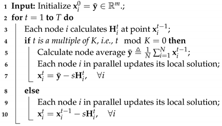Algorithm 1 is essentially the same as FedAvg described in [13], except that the stochastic gradient ${\mathbf{H}}_i^t$ is computed on $g_i(·)$, the expected loss for the newly defined q-FFL objective.

Fix iteration index t, we define

$${\overline{\mathbf{x}}}^t\triangleq {\displaystyle \frac{1}{N}}\sum _{i=1}^N{\mathbf{x}}_i^t$$

as the average of local solution ${\mathbf{x}}_i^t$ over all N nodes. It is immediate that

$${\overline{\mathbf{x}}}^t={\overline{\mathbf{x}}}^{t-1}-s{\displaystyle \frac{1}{N}}\sum _{i=1}^N{\mathbf{H}}_i^t={\overline{\mathbf{x}}}^{t-1}-s{\displaystyle \frac{1}{N}}\sum _{i=1}^N{f}_i^q\left({\mathbf{x}}_i^{t-1}\right){\mathbf{G}}_i^t$$

The proof starts from the descent lemma and the L-smoothness assumption. Then we bound the generated quadratic term and cross term using the same technique from [12]. And lastly, through a telescoping sum, we get an upper bound on the (average) expected square gradient norm. The following useful lemma relates client drift $\mathbb{E}[\parallel {\overline{\mathbf{x}}}^t-{\mathbf{x}}_i^t{\parallel }^2]$ and node synchronization interval K. Table 1 summarizes our notation.

Lemma 1: (Client drift) Under Assumption 1, the algorithm ensures

$$\mathbb{E}[\parallel {\mathbf{x}}_i^t-{\overline{\mathbf{x}}}^t{\parallel }^2]\le 4s^2{K}^2{G}^2{M}^{2q},\forall i,\forall t$$

where s is the constant stepsize, $G,M$ are constant defined in Assumption 1, and q is the fairness parameter.

Proof. 

$${\mathbf{x}}_i^t=\overline{\mathbf{y}}-s\sum _{\tau =t_0+1}^t{\mathbf{H}}_i^{\tau }$$

$${\overline{\mathbf{x}}}^t=\sum _{i=1}^N{\mathbf{x}}_i^t=\overline{\mathbf{y}}-s\sum _{\tau =t_0+1}^t{\displaystyle \frac{1}{N}}\sum _{i=1}^N{\mathbf{H}}_i^{\tau }$$

Thus, we have

$$\begin{array}{cc}\hfill & \mathbb{E}[\parallel {\mathbf{x}}_i^t-{\overline{\mathbf{x}}}^t{\parallel }^2]\hfill \\ \hfill & =\mathbb{E}[\parallel s\sum _{\tau =t_0+1}^t{\displaystyle \frac{1}{N}}\sum _{i=1}^N{\mathbf{H}}_i^{\tau }-s\sum _{\tau =t_0+1}^t{\mathbf{H}}_i^{\tau }{\parallel }^2]\hfill \\ \hfill & =s^2\mathbb{E}[\parallel \sum _{\tau =t_0+1}^t{\displaystyle \frac{1}{N}}\sum _{i=1}^N{\mathbf{H}}_i^{\tau }-\sum _{\tau =t_0+1}^t{\mathbf{H}}_i^{\tau }{\parallel }^2]\hfill \\ \hfill & \le 2s^2\mathbb{E}[\parallel \sum _{\tau =t_0+1}^t{\displaystyle \frac{1}{N}}\sum _{i=1}^N{\mathbf{H}}_i^{\tau }{\parallel }^2+\parallel \sum _{\tau =t_0+1}^t{\mathbf{H}}_i^{\tau }{\parallel }^2]\hfill \\ \hfill & \le 2s^2(t-t_0)\mathbb{E}[\sum _{\tau =t_0+1}^t\parallel {\displaystyle \frac{1}{N}}\sum _{i=1}^N{\mathbf{H}}_i^{\tau }{\parallel }^2+\parallel \sum _{\tau =t_0+1}^t{\mathbf{H}}_i^{\tau }{\parallel }^2]\hfill \\ \hfill & \le 2s^2(t-t_0)\mathbb{E}[\sum _{\tau =t_0+1}^t({\displaystyle \frac{1}{N}}\sum _{i=1}^N\parallel {\mathbf{H}}_i^{\tau }{\parallel }^2)+\parallel \sum _{\tau =t_0+1}^t{\mathbf{H}}_i^{\tau }{\parallel }^2]\hfill \\ \hfill & \le 2s^2(t-t_0)\mathbb{E}[\sum _{\tau =t_0+1}^t({\displaystyle \frac{1}{N}}\sum _{i=1}^N{f}_i^{2q}\left({\mathbf{x}}_i^{t-1}\right)\parallel f_i^q\left({\mathbf{x}}_i^{t-1}\right){\mathbf{G}}_i^{\tau }{\parallel }^2)+\parallel \sum _{\tau =t_0+1}^t{f}_i^q\left({\mathbf{x}}_i^{t-1}\right){\mathbf{G}}_i^{\tau }{\parallel }^2]\hfill \\ \hfill & \le 4s^2{K}^2{G}^2{M}^{2q}\hfill \end{array}$$

   □

Theorem 1. Under Assumption 1, if $0<s\le {\displaystyle \frac{1}{L}}$ in the Algorithm, then for all $T\ge 1$, we have

$${\displaystyle \frac{1}{T}}\sum _{i=1}^T\mathbb{E}[\parallel \nabla g\left({\overline{\mathbf{x}}}^{t-1}\right){\parallel }^2]\le {\displaystyle \frac{2}{sT}}(g\left({\overline{\mathbf{x}}}^0\right)-f^{*})+4s^2{K}^2{G}^2{L}^2{M}^{4q}+{\displaystyle \frac{Ls{\sigma }^2{M}^{2q}}{N}}$$

where $f^{*}$ is the minimum value of the problem.

Proof. 

From L-smoothness and descent lemma:

$$\mathbb{E}[g\left({\overline{\mathbf{x}}}^t\right)]\le \mathbb{E}[g\left({\overline{\mathbf{x}}}^{t-1}\right)]+\mathbb{E}[\langle \nabla g\left({\overline{\mathbf{x}}}^{t-1}\right),{\overline{\mathbf{x}}}^t-{\overline{\mathbf{x}}}^{t-1}\rangle ]+{\displaystyle \frac{L}{2}}\mathbb{E}[\parallel {\overline{\mathbf{x}}}^t-{\overline{\mathbf{x}}}^{t-1}{\parallel }^2]$$

(3)

For the quadratic term,

$$\begin{array}{cc}\hfill & \mathbb{E}[\parallel {\overline{\mathbf{x}}}^t-{\overline{\mathbf{x}}}^{t-1}{\parallel }^2]\hfill \\ \hfill & =s^2\mathbb{E}[\parallel {\displaystyle \frac{1}{N}}\sum _{i=1}^N{\mathbf{H}}_i^t{\parallel }^2]\hfill \\ \hfill & ={\displaystyle \frac{s^2}{N^2}}\sum _{i=1}^N\mathbb{E}[\parallel {\mathbf{H}}_i^t-\nabla g_i\left({\mathbf{x}}_i^{t-1}\right){\parallel }^2]+s^2\mathbb{E}[\parallel {\displaystyle \frac{1}{N}}\sum _{i=1}^N\nabla g_i\left({\mathbf{x}}_i^{t-1}\right){\parallel }^2]\hfill \\ \hfill & ={\displaystyle \frac{s^2}{N^2}}\sum _{i=1}^N\mathbb{E}[\parallel f_i^q\left({\mathbf{x}}_i^{t-1}\right)({\mathbf{G}}_i^t-\nabla f_i\left({\mathbf{x}}_i^{t-1}\right)){\parallel }^2]+s^2\mathbb{E}[\parallel {\displaystyle \frac{1}{N}}\sum _{i=1}^N\nabla f_i\left({\mathbf{x}}_i^{t-1}\right)f_i^q\left({\mathbf{x}}_i^{t-1}\right){\parallel }^2]\hfill \\ \hfill & \le {\displaystyle \frac{s^2{M}^{2q}}{N^2}}\sum _{i=1}^N\mathbb{E}[\parallel {\mathbf{G}}_i^t-\nabla f_i\left({\mathbf{x}}_i^{t-1}\right){\parallel }^2]+s^2{M}^{2q}\mathbb{E}[\parallel {\displaystyle \frac{1}{N}}\sum _{i=1}^N\nabla f_i\left({\mathbf{x}}_i^{t-1}\right){\parallel }^2]\hfill \\ \hfill & \le {\displaystyle \frac{1}{N}}{s}^2{\sigma }^2{M}^{2q}+s^2{M}^{2q}\mathbb{E}[\parallel {\displaystyle \frac{1}{N}}\sum _{i=1}^N\nabla f_i\left({\mathbf{x}}_i^{t-1}\right){\parallel }^2]\hfill \end{array}$$

(4)

For the cross term:

$$\begin{array}{cc}\hfill & \mathbb{E}[\langle \nabla g\left({\overline{\mathbf{x}}}^{t-1}\right),{\overline{\mathbf{x}}}^t-{\overline{\mathbf{x}}}^{t-1}\rangle ]\hfill \\ \hfill & =-s\mathbb{E}[\langle \nabla g\left({\overline{\mathbf{x}}}^{t-1}\right),{\displaystyle \frac{1}{N}}\sum _{i=1}^N{f}_i^q\left({\mathbf{x}}_i^{t-1}\right)\nabla f_i\left({\mathbf{x}}_i^{t-1}\right)\rangle ]\hfill \\ \hfill & =-{\displaystyle \frac{s}{2}}\mathbb{E}[\parallel \nabla g\left({\overline{\mathbf{x}}}^{t-1}\right){\parallel }^2+\parallel {\displaystyle \frac{1}{N}}\sum _{i=1}^N{f}_i^q\left({\mathbf{x}}_i^{t-1}\right)\nabla f_i\left({\mathbf{x}}_i^{t-1}\right){\parallel }^2-\parallel \nabla g\left({\overline{\mathbf{x}}}^{t-1}\right)-{\displaystyle \frac{1}{N}}\sum _{i=1}^N{f}_i^q\left({\mathbf{x}}_i^{t-1}\right)\nabla f_i\left({\mathbf{x}}_i^{t-1}\right){\parallel }^2]\hfill \end{array}$$

(5)

Substituting $\left(4\right)$ and $\left(5\right)$ into $\left(3\right)$ yields

$$\begin{array}{cc}\hfill & \mathbb{E}[g\left({\overline{\mathbf{x}}}^t\right)]\hfill \\ \hfill & \le \mathbb{E}[g\left({\overline{\mathbf{x}}}^{t-1}\right)]-{\displaystyle \frac{s-s^{2}L}{2}}\mathbb{E}[\parallel {\displaystyle \frac{1}{N}}\sum _{i=1}^N{f}_i^q\left({\mathbf{x}}_i^{t-1}\right)\nabla f_i\left({\mathbf{x}}_i^{t-1}\right){\parallel }^2]-{\displaystyle \frac{s}{2}}\mathbb{E}[\parallel \nabla g\left({\overline{\mathbf{x}}}^{t-1}\right){\parallel }^2]\hfill \\ \hfill & +{\displaystyle \frac{s}{2}}\mathbb{E}[\parallel \nabla g\left({\overline{\mathbf{x}}}^{t-1}\right)-{\displaystyle \frac{1}{N}}\sum _{i=1}^N{f}_i^q\left({\mathbf{x}}_i^{t-1}\right)\nabla f_i\left({\mathbf{x}}_i^{t-1}\right){\parallel }^2]+{\displaystyle \frac{L{s}^2{\sigma }^2{M}^{2q}}{2N}}\hfill \end{array}$$

(6)

$$\begin{array}{cc}\hfill & \mathbb{E}[\parallel \nabla g\left({\overline{\mathbf{x}}}^{t-1}\right)-{\displaystyle \frac{1}{N}}\sum _{i=1}^N{f}_i^q\left({\mathbf{x}}_i^{t-1}\right)\nabla f_i\left({\mathbf{x}}_i^{t-1}\right){\parallel }^2]\hfill \\ \hfill & =\mathbb{E}[\parallel {\displaystyle \frac{1}{N}}\sum _{i=1}^N\nabla f_i\left({\overline{\mathbf{x}}}^{t-1}\right)f_i^q\left({\overline{\mathbf{x}}}^{t-1}\right)-{\displaystyle \frac{1}{N}}\sum _{i=1}^N\nabla f_i\left({\mathbf{x}}_i^{t-1}\right)f_i^q\left({\mathbf{x}}_i^{t-1}\right){\parallel }^2]\hfill \\ \hfill & \le {\displaystyle \frac{1}{N}}\mathbb{E}[\sum _{i=1}^N\parallel \nabla f_i\left({\overline{\mathbf{x}}}^{t-1}\right)f_i^q\left({\overline{\mathbf{x}}}^{t-1}\right)-\nabla f_i\left({\mathbf{x}}_i^{t-1}\right)f_i^q\left({\mathbf{x}}_i^{t-1}\right){\parallel }^2]\hfill \\ \hfill & \le M^{2q}{\displaystyle \frac{1}{N}}\mathbb{E}[\sum _{i=1}^N\parallel \nabla f_i\left({\overline{\mathbf{x}}}^{t-1}\right)-\nabla f_i\left({\mathbf{x}}_i^{t-1}\right){\parallel }^2]\hfill \\ \hfill & \le M^{2q}{L}^2{\displaystyle \frac{1}{N}}\sum _{i=1}^N\mathbb{E}[\parallel {\overline{\mathbf{x}}}^{t-1}-{\mathbf{x}}_i^{t-1}{\parallel }^2]\hfill \\ \hfill & \le 4s^2{K}^2{G}^2{L}^2{M}^{4q}\hfill \end{array}$$

(7)

Plugging $\left(7\right)$ back into $\left(6\right)$ and let $0<s\le {\displaystyle \frac{1}{L}}$, we have

$$\mathbb{E}[g\left({\overline{\mathbf{x}}}^t\right)]\le \mathbb{E}[g\left({\overline{\mathbf{x}}}^{t-1}\right)]-{\displaystyle \frac{s}{2}}\mathbb{E}[\parallel \nabla g\left({\overline{\mathbf{x}}}^{t-1}\right){\parallel }^2]+2s^3{K}^2{G}^2{L}^2{M}^{4q}+{\displaystyle \frac{L{s}^2{\sigma }^2{M}^{2q}}{2N}}$$

(8)

Dividing both sides of $\left(8\right)$ by $s/2$ and rearranging terms yields

$$\mathbb{E}[\parallel \nabla g\left({\overline{\mathbf{x}}}^{t-1}\right){\parallel }^2]\le {\displaystyle \frac{2}{s}}(\mathbb{E}[g\left({\overline{\mathbf{x}}}^{t-1}\right)]-\mathbb{E}[g\left({\overline{\mathbf{x}}}^t\right)])+4s^2{K}^2{G}^2{L}^2{M}^{4q}+{\displaystyle \frac{Ls{\sigma }^2{M}^{2q}}{N}}$$

(9)

Summing over $t\in \{1,\cdots ,T\}$ and dividing both sides by T yields

$$\begin{array}{cc}\hfill & {\displaystyle \frac{1}{T}}\sum _{i=1}^T\mathbb{E}[\parallel \nabla g\left({\overline{\mathbf{x}}}^{t-1}\right){\parallel }^2]\hfill \\ \hfill & \le {\displaystyle \frac{2}{sT}}(g\left({\overline{\mathbf{x}}}^0\right)-\mathbb{E}[f\left({\overline{\mathbf{x}}}^T\right)])+4s^2{K}^2{G}^2{L}^2{M}^{4q}+{\displaystyle \frac{Ls{\sigma }^2{M}^{2q}}{N}}\hfill \\ \hfill & \le {\displaystyle \frac{2}{sT}}(g\left({\overline{\mathbf{x}}}^0\right)-f^{*})+4s^2{K}^2{G}^2{L}^2{M}^{4q}+{\displaystyle \frac{Ls{\sigma }^2{M}^{2q}}{N}}\hfill \end{array}$$

   □

The next corollary follows by substituting suitable $s,K$ values into Theorem 1.

Corollary 1. Consider the problem under Assumption 1. Let $T\ge N$.

1. If we choose $s={\displaystyle \frac{\sqrt{N}}{L\sqrt{T}}}$ in the Algorithm, then we have ${\displaystyle \frac{1}{T}}{\sum }_{i=1}^T\mathbb{E}[\parallel \nabla g\left({\overline{\mathbf{x}}}^{t-1}\right){\parallel }^2]\le {\displaystyle \frac{2L}{\sqrt{NT}}}\left(g({\overline{\mathbf{x}}}^0-g^{*})\right)+{\displaystyle \frac{4N}{T}}{K}^2{G}^2{M}^{2q}+{\displaystyle \frac{1}{\sqrt{NT}}}{\sigma }^2{M}^{2q}$.

2. If we further choose $K\le {\displaystyle \frac{T^{1/4}}{N^{3/4}}}$, then ${\displaystyle \frac{1}{T}}{\sum }_{i=1}^T\mathbb{E}[\parallel \nabla g\left({\overline{\mathbf{x}}}^{t-1}\right){\parallel }^2]\le {\displaystyle \frac{2L}{\sqrt{NT}}}\left(g({\overline{\mathbf{x}}}^0-g^{*})\right)+{\displaystyle \frac{4}{\sqrt{NT}}}{G}^2{M}^{2q}+{\displaystyle \frac{1}{\sqrt{NT}}}{\sigma }^2{M}^{2q}=\mathcal{O}\left({\displaystyle \frac{1}{\sqrt{NT}}}\right)$ where $g^{*}$ is the minimum value of the problem.

With proper assumptions, FedAvg can achieve the same convergence rate on the objective of q-fair federated learning as the original objective.

3. Fair Incentive Mechanism Design Through Stackelberg Game Settings

Most of the studies in Federated Learning (FL) have been focused on convergence rate and stationary gap of optimization algorithms. However, designing mechanisms motivating local devices known as clients in terms of FL to collaborate in global model training has not received enough attention. [14] devised an incentive mechanism in a Stackelberg game setting, and proved the existence of a unique Nash equilibrium.

In the first stage of a Stackelberg game, the parameter server (leader) strives to convince clients (followers) to participate in the training of a global model by declaring a total payment of $\tau >0$. Next in the second stage, participants decide about how much local data they are going to train. [14] proved that for any $\tau$, the second-stage game has a unique Nash equilibrium, and furthermore, there exists a unique Stackelberg equilibrium for the game. The edge nodes also incur two costs, communication cost $c_n^{com}$ and computation cost $c_n^{cmp}$ given their training data set size $x_n$.

Based on works of [14] and [15], we add a fairness coefficient to the utility functions of clients in a federated learning incentive mechanism design with the hope that this additive term causes more fair allocation of resources to clients. [15] argues that the global fairness of a model considers the full dataset across all clients while in local fairness performance measurement, data sets are typically non-iid. To address this issue, they propose a global and local fairness metric, i.e.,

$$F_{global}=Pr(\widehat{Y}=1|A=0,Y=1)-Pr(\widehat{Y}=1|A=1,Y=1)$$

Where $\widehat{Y}$ is a trained classifier and A is a group, let’s say, gender group. The ideal amount of the above metric is zero meaning that the true positive rate of the above metric should be equal regardless of the gender, male or female. The local fairness metric is defined as:

$$F_k=Pr(\widehat{Y}=1|A=0,Y=1,C=k)-Pr(\widehat{Y}=1|A=1,Y=1,C=k)$$

Where C denotes the $k^{th}$ client and for $F_k$, $k^{th}$ clients data set and distribution have been considered [15]. Furthermore, in FedAvg, [13], we have weights when doing the conventional global updates, i.e., $w_k^t={\displaystyle \frac{n_k}{{\sum }_k{n}_k}}$. Particularly, [15] discusses that these naive aggregation weights disfavour clients with lower data set sizes and they propose the following modified version of aggregation weights to achieve global fairness as follows:

$$w_k^t=exp(-\beta |F_k^t-F_{global}^t\left|\right){\displaystyle \frac{n_k}{{\sum }_k{n}_k}}$$

We adopted this approach and integrated it into the work of [14]. Notations and proofs of the existence of Nash equilibrium in the modified version of this work have been demonstrated in what follows.

The utility of each client is modified by adding a fairness term to it, i.e.,

$$u(n,-n)=exp\left({\gamma }_n\right){\displaystyle \frac{x_n}{{\sum }_i{x}_i}}\tau -C_n^{com}{x}_n-C_n^{cmp}{x}_n$$

Where ${\gamma }_n=-\beta |F_k^t-F_{global}^t|$. To maximize the utility of each client, we take the derivative of the utility function and put it equal to zero, i.e.,

$$u^{\prime }(n,-n)=exp\left({\gamma }_n\right){\displaystyle \frac{{\sum }_i{x}_i-x_n}{{\left({\sum }_i{x}_i\right)}^2}}\tau -C_n^{com}-C_n^{cmp}=0$$

To ensure that the answers to the above equation are not saddle points, we derive the second derivative w.r.t. $x_n$, i.e.,

$$u"(n,-n)={\displaystyle \frac{exp\left({\gamma }_n\right)(-2{\sum }_i{x}_i)({\sum }_i{x}_i-x_n}{{(\sum x_i)}^4}})\tau <0$$

This means that the utility function is strictly concave and the solutions are global optimal, i.e.,

$$x_n={\left({(C_n^{com}+C_n^{cmp})}^{-1}\tau exp\left({\gamma }_n\right)\left(\sum _{i\ne n}{x}_i\right)\right)}^{{\displaystyle \frac{1}{2}}}-\sum _{i\ne n}{x}_i$$

However, there is a limitation on the amount of clients’ contributions, i.e., it cannot exceed $d_n$, and it depends also on the $\tau$, hence, we have:

$$x_n=\left\{\begin{array}{cc}0\hfill & \tau <{\displaystyle \frac{\left({\sum }_{i\ne n}{x}_i\right)(C_n^{com}+C_n^{cmp})}{exp\left({\gamma }_n\right)}}\hfill \\ {\left({(C_n^{com}+C_n^{cmp})}^{-1}\tau exp\left({\gamma }_n\right)\left(\sum _{i\ne n}{x}_i\right)\right)}^{{\displaystyle \frac{1}{2}}}-\sum _{i\ne n}{x}_i\hfill & x_n\in (0,d_n)\hfill \\ d_n\hfill & \mathrm{Otherwise}\hfill \end{array}\right.$$

Then, one can derive the best response from the followers, and clients, independent of other clients, as follows:

$$\sum _n{x}_n^{*}=\sqrt{{\displaystyle \frac{\tau \left({\sum }_{n\ne m}{x}_n^{*}\right)exp\left({\gamma }_m\right)}{C_m^{com}+C_m^{cpm}}}}$$

Then observe that,

$$x_1^{*}=a-{\displaystyle \frac{a^2(C_1^{com}+C_1^{cmp})}{\tau exp\left({\gamma }_1\right))}}$$

Finally, considering the $M^{th}$ client,

$$x_M^{*}=a-{\displaystyle \frac{a^2(C_M^{com}+C_M^{cmp})}{\tau exp\left({\gamma }_M\right))}}$$

Observe that summing both sides of equations from 1 to M, yields:

$$a=Ma-\sum _{n=1}^M{\displaystyle \frac{a^2(C_n^{com}+C_n^{cmp})}{\tau exp\left({\gamma }_n\right)}}$$

implying that,

$$a={\displaystyle \frac{M-1}{{\sum }_{n=1}^M\frac{C_n^{com}+C_n^{cmp}}{\tau exp\left({\gamma }_n\right)}}}$$

Finally, observe that:

$$x_m^{*}={\displaystyle \frac{M-1}{{\sum }_{n=1}^M\frac{C_n^{com}+C_n^{cpm}}{\tau \left(exp\left(X_n\right)\right)}}}-{\left({\displaystyle \frac{M-1}{{\sum }_{n=1}^M\frac{C_n^{com}+C_n^{cpm}}{\tau \left(exp\left(X_n\right)\right)}}}\right)}^2.{\displaystyle \frac{C_m^{com}+C_m^{cpm}}{\tau exp\left({\gamma }_m\right)}}$$

So far, we have found the best responses of followers. At this point, the leader knows that whatever the payment is there exists a unique equilibrium, the leader strives to derive the maximum profit by best tuning $\tau$ i.e., $u\left(\tau \right)=\lambda g\left({\sum }_n{x}_n^{*}\right)-\tau$ is the parameter serverer utility function as defined in [14].

$${\displaystyle \frac{\partial u\left(\tau \right)}{\partial \tau }}=\lambda g^{\prime }\left(X\right){\displaystyle \frac{\partial X}{\partial \tau }}-1$$

and we have that

$${\displaystyle \frac{\partial x_m^{*}}{\partial \tau }}=\left({\displaystyle \frac{M-1}{{\sum }_n\frac{C_n^{com}+C_n^{cmp}}{exp\left(x_n\right)}}}\right)-{\left({\displaystyle \frac{M-1}{{\sum }_n\frac{C_n^{com}+C_n^{cmp}}{exp\left(x_n\right)}}}\right)}^2{\displaystyle \frac{C_m^{com}+C_m^{cmp}}{exp\left(x_m\right)}}$$

And,

$${\displaystyle \frac{{\partial }^2{x}_m^{*}}{\partial {\tau }^2}}=0$$

Hence, we have,

$${\displaystyle \frac{\partial u\left(\tau \right)}{\partial \tau }}=\lambda g^{\prime }\left(x\right)\left(\sum _{m=1}^N\left({\displaystyle \frac{M-1}{{\sum }_n\frac{C_n^{com}+C_n^{cmp}}{exp\left(x_n\right)}}}-{\left({\displaystyle \frac{M-1}{{\sum }_n\frac{C_n^{com}+C_n^{cmp}}{exp\left(x_n\right)}}}\right)}^2{\displaystyle \frac{C_m^{com}+C_m^{cmp}}{exp\left(x_m\right)}}\right)-1\right)$$

Given that ${\displaystyle \frac{{\partial }^{2}g\left(x\right)}{\partial x^2}}<0$, we have,

$${\displaystyle \frac{{\partial }^{2}u\left(\tau \right)}{\partial {\tau }^2}}=\lambda {\displaystyle \frac{{\partial }^{2}g\left(x\right)}{\partial x^2}}{\left(\sum _{m=1}^N\left({\displaystyle \frac{M-1}{{\sum }_n\frac{C_n^{com}+C_n^{cmp}}{exp\left(x_n\right)}}}-\left({\displaystyle \frac{M-1}{{\sum }_n\frac{C_n^{com}+C_n^{cmp}}{exp\left(x_n\right)}}}\right){\displaystyle \frac{C_m^{com}+C_m^{cmp}}{exp\left(x_m\right)}}\right)\right)}^2<0$$

Since $u\left(\tau \right)$ is a concave function and its value is equal to zero when $\tau =0$, then it has a unique maximize, and the proof is done.

4. Summary

In this project, we studied the fairness issue in federated learning. Two different notions of fairness were examined: $\left(1\right)$ fair (uniform) model performance across local clients and $\left(2\right)$ fair incentive mechanism. To achieve the first type of fairness, a novel optimization objective q-FFL was introduced. We tried to fit this federated learning task into the FedAvg framework and derived the convergence rate.

At first, we thought we had proven it by following a similar procedure from previous literature. However, after a careful examination of the new objective function, we realized that some parts in the proof procedure of [12] cannot be used in this case due to the change of objective. For example, we do not know ${\mathbb{E}}_{{\zeta }_i\sim {\mathcal{D}}_i}[{\displaystyle \frac{1}{q+1}}{F}_i^q(\mathbf{x};{\zeta }_i)]$ when only knowing ${\mathbb{E}}_{{\zeta }_i\sim {\mathcal{D}}_i}[F_i(\mathbf{x};{\zeta }_i)]=f_i\left(\mathbf{x}\right)$. Therefore, we could not use SGD for a local update as in FedAvg. Either we need more assumptions or find a suitable structure of $F_i\left(\mathbf{x}\right)$ to make Theorem 1 hold.

As for the fairness in the incentive mechanism, we modeled the training process as a Stackelberg game where the server is treated as the leader and the clients are followers. Once the server announces a payment for training the global model, the followers decide the amount of data (and effort) they would like to contribute to the training task to maximize their payment. We have proven that the system could reach a unique Stackelberg equilibrium.

References

- Nematirad, R.; Ardehali, M.; Khorsandi, A.; Mahmoudian, A. Optimization of Residential Demand Response Program Cost with Consideration for Occupants Thermal Comfort and Privacy. IEEE Access 2024. [CrossRef]
- Talebi, A. A multi-objective mixed integer linear programming model for supply chain planning of 3D printing. 2024. arXiv:2408.05213.
- Varmaz, A.; Fieberg, C.; Poddig, T. Portfolio optimization for sustainable investments. Annals of Operations Research 2024, pp. 1–26.
- Talebi, A.; Haeri Boroujeni, S.P.; Razi, A. Integrating random regret minimization-based discrete choice models with mixed integer linear programming for revenue optimization. Iran Journal of Computer Science 2024, pp. 1–15.
- Archetti, C.; Peirano, L.; Speranza, M.G. Optimization in multimodal freight transportation problems: A Survey. European Journal of Operational Research 2022, 299, 1–20. [CrossRef]
- Talebi, A. Simulation in discrete choice models evaluation: SDCM, a simulation tool for performance evaluation of DCMs. 2024. arXiv:2407.17014.
- Nematirad, R.; Pahwa, A.; Natarajan, B. A Novel Statistical Framework for Optimal Sizing of Grid-Connected Photovoltaic–Battery Systems for Peak Demand Reduction to Flatten Daily Load Profiles. Solar. MDPI, 2024, Vol. 4, pp. 179–208.
- Nematirad, R.; Pahwa, A.; Natarajan, B.; Wu, H. Optimal sizing of photovoltaic-battery system for peak demand reduction using statistical models. Frontiers in Energy Research 2023, 11, 1297356. [CrossRef]
- Soleymani, S.; Talebi, A. Forecasting solar irradiance with geographical considerations: integrating feature selection and learning algorithms. Asian Journal of Social Science 2024, 8, 5.
- Talebi, A. Convergence Rate Analysis of Non-I.I.D. SplitFed Learning with Partial Worker Participation and Auxiliary Networks. Preprints 2024. [CrossRef]
- Li, T.; Sanjabi, M.; Beirami, A.; Smith, V. Fair Resource Allocation in Federated Learning. International Conference on Learning Representations, 2020.
- Yu, H.; Yang, S.; Zhu, S. Parallel Restarted SGD with Faster Convergence and Less Communication: Demystifying Why Model Averaging Works for Deep Learning. Proceedings of the AAAI Conference on Artificial Intelligence 2019, 33, 5693–5700. [CrossRef]
- McMahan, B.; Moore, E.; Ramage, D.; Hampson, S.; y Arcas, B.A. Communication-efficient learning of deep networks from decentralized data. Artificial intelligence and statistics. PMLR, 2017, pp. 1273–1282.
- Zhan, Y.; Li, P.; Qu, Z.; Zeng, D.; Guo, S. A Learning-Based Incentive Mechanism for Federated Learning. IEEE Internet of Things Journal 2020, 7, 6360–6368. [CrossRef]
- Ezzeldin, Y.H.; Yan, S.; He, C.; Ferrara, E.; Avestimehr, S. Fairfed: Enabling group fairness in federated learning. 2021. arXiv:2110.00857.
- Karimireddy, S.P.; Kale, S.; Mohri, M.; Reddi, S.; Stich, S.; Suresh, A.T. Scaffold: Stochastic controlled averaging for federated learning. International Conference on Machine Learning. PMLR, 2020, pp. 5132–5143.
Disclaimer/Publisher’s Note: The statements, opinions and data contained in all publications are solely those of the individual author(s) and contributor(s) and not of MDPI and/or the editor(s). MDPI and/or the editor(s) disclaim responsibility for any injury to people or property resulting from any ideas, methods, instructions or products referred to in the content. |
© 2024 by the authors. Licensee MDPI, Basel, Switzerland. This article is an open access article distributed under the terms and conditions of the Creative Commons Attribution (CC BY) license (http://creativecommons.org/licenses/by/4.0/).
Copyright: This open access article is published under a Creative Commons CC BY 4.0 license, which permit the free download, distribution, and reuse, provided that the author and preprint are cited in any reuse.