
Submitted:
12 February 2025
Posted:
12 February 2025
You are already at the latest version
Abstract
This study investigates the tanker freight market and its complex transformation from 1998 to 2024, uncovering a high degree of multifractality and a complex market structure shaped by temporal correlations and inherent volatility. Using multifractal dynamics analyzed through multifractal detrended fluctuation analysis (MF-DFA) and multifractal detrending moving average (MF-DMA), we explore how key external factors drive market complexity, including economic disturbances (the 2008 Financial Crisis), technological innovations (the 2014 Shale Oil Revolution), supply chain disruptions (the COVID-19 pandemic), and geopolitical uncertainties (the Russia-Ukraine conflict). Building on this, a predictive framework is introduced, leveraging the Baltic Dirty Tanker Index (BDTI) to forecast Brent oil prices. By integrating multifractal analysis with machine learning models, such as XGBoost, LightGBM, and CatBoost, the framework captures complexity transformation across these four major global events. Results demonstrate the potential of combining multifractal analysis with advanced machine learning models to improve forecasting accuracy and provide actionable insights during periods of heightened market volatility.
Keywords:
Tanker freight market
; Multifractal dynamics
; Brent oil prices
; Temporal correlations
; Complexity Transformation
; Machine learning models
Introduction
The intricate dynamics of the global tanker freight market have long been a subject of interest for both academicians and industry practitioners due to its critical role in the shipping market, i.e. Adland and Cullinane [1], Zhang and Zeng [2], and Sun et al [3]. This market exhibits complex behaviors that are influenced by a multitude of factors, including geopolitical events [4,5,6], economic conditions [7], technological innovations, and environmental policies [8]. The study of these dynamics is further complicated by the market's inherent volatility and the interplay of various scales of temporal correlations [9,10]. Examination of market trends assists stakeholders in harnessing shifts to their advantage, while the progressive integration of technology reshapes market operations [11,12,13,14,15,16,17,18]. Despite the growing interest in this field, there remain several gaps and challenges that warrant further investigation. A need for a more nuanced understanding of the causal relationships between the multifractal dynamics of the tanker freight market and the various external factors that influence it, such as geopolitical tensions, economic cycles, and environmental policies, see Gao and Zhang [4], and Chen et al. [9]. There is also a need for more interdisciplinary research that integrates insights from complexity economics, financial engineering, and operations research to develop more sophisticated methodologies for analyzing and managing the risks associated with changing dynamics in the tanker freight market [19,20,21].
Complexity economics provides a framework for interdisciplinary research of economics, information, physics and operations [22,23,24]. It acknowledges the differences among agents, their imperfect information, and the dynamic nature of economic systems, providing significant insights applicable to both the fields of information and economics [25,26,27,28], including the energy and tanker freight market [4,12]. A series of models for fractals are developed as an effective tool for complexity economics studies. Fractals, known for their fragmented and rough geometric shapes, have the fascinating property of self-similarity, allowing them to be broken down into smaller parts that closely resemble the whole[29,30]. A variety of methodologies have been devised to analyze fractal attributes. One of the first was the rescaled range analysis by Hurst, which, however, faces challenges in assessing long-range dependencies in nonstationary series [31]. To tackle multi-affine fractal exponents and correlation coefficients, Castro et al. introduced a novel approach [32]. Around the same time, Peng et al. firstly constructed a different method called detrended fluctuation analysis (DFA) to discern long-term correlations within data [33]. While DFA provided a valuable tool, it fell short when it came to multi-scale and fractal elements in time series that demonstrated more complex, non-monofractal scaling. To bridge this gap, multifractal detrended fluctuation analysis (MF-DFA) came into play, advanced by Kantelhardt et al. as a multifaceted extension of the DFA method [34]. MF-DFA has proven to be a robust tool for multifractal characterization and has been used across various stochastic analysis contexts [35,36]. In parallel, the detrending moving average (DMA) technique gained traction for its effectiveness in evaluating long memory in nonstationary time series, applicable to both real and theoretical data samples [37,38,39]. By focusing on the moving average function of a series and building on the moving average methodology, DMA excels in discerning scaling properties within time series data [40]. MF-DMA extended DMA to higher-dimensional versions. It is a quantitative analysis delving into the spurious multifractality induced by fat-tailed probability distributions in time series, providing critical insights into distinguishing true multifractality arising from nonlinear correlations from spurious effects generated by distribution shapes [41,42]. Kwapien et al. use analytical arguments as well as numerical illustrations on the interesting question of the origin of the multifractality in time series [43]. They get the conclusion that true multifractality in time series comes from temporal correlations.
The array of studies on tanker freight rate volatility represents a vital component of maritime economics, with ramifications extending into the broader global economy, delve into the interplay between numerous variables affecting freight rates, such as crude oil prices, charter rates, fleet size, and policy changes [13,14,15,16,17,18,19,44]. Multifractal analysis has emerged as a new trend in these studies, gaining traction due to its ability to capture the asymmetric nature of market risks, demonstrating different magnitudes of response to upward and downward trends and uncovers various scaling behaviors within the data[45,46]. Multifractality helps to recognize the freight rates which exhibit a spectrum of fractal characteristics, not just a single pattern of fluctuations [47,48,49,50]. It accounts for both small and large movements, providing a nuanced perspective on data correlations, especially under turbulent market conditions like those experienced during the 2008 world finance risk and the COVID-19 pandemic [4,12,46]. This study tries to comprehend the intricate, multifaceted nature of the market to design strategies that buffer the fallout from unpredictable market shifts or crises, provide a comprehensive understanding of the market's complexity and its evolution over time.
The research is driven by the following key questions: (a) How has the multifractal nature of the tanker freight market evolved across the two distinct periods, and what does this evolution signify in terms of market behavior and systemic risks? (b) What role do temporal correlations and inherent volatility play in shaping the complex structure of the market, and how do these factors contribute to the observed multifractal dynamics? (c) How do external factors such as regulatory changes, economic disturbances, technological innovation, and environmental concerns influence the complexity and multifractal characteristics of the tanker freight market? (d) Can tanker freight rates, specifically the Baltic Dirty Tanker Index (BDTI), be used to predict Brent oil prices during periods of heightened market complexity, and how do multifractal features enhance the predictive power of such models?
The research presented in this manuscript is motivated by the need to delve into the complex transformation of the Baltic Clean and Dirty Tankers markets from 1998 to 2023, with a particular focus on the multifractal characteristics that define the market's structure and behavior. Here, we apply the MF-DFA method to characterize the observations of clean and dirty tanker freight rates and the most concerned routes of TC2 and TD7 from Jan. 28, 1998, to Jan. 12, 2024. To describe the market pattern after larger fluctuations, we analyze Period I (1998–2010) and Period II (2010–2024). To better explain the multifractality in the BCTI and BDTI series, we apply the MF-DMA method to quantify the three components, including linear correlation, nonlinear correlation, and fat-tailed probability distribution.
Building on this foundational analysis, we further extend the scope of our research to explore the predictive potential of freight rates in forecasting Brent oil prices, particularly during periods of heightened market volatility and complexity. Traditionally, most studies have focused on forecasting freight rates based on oil price movements, reflecting the conventional economic logic that oil prices drive downstream costs, including shipping. However, freight rates, due to their responsiveness to supply-demand dynamics, vessel utilization rates, and macroeconomic shifts, may serve as valuable leading indicators for oil prices. This study, therefore, adopts an innovative perspective by investigating whether BDTI can predict Brent oil prices and how multifractal features contribute to the accuracy of such predictions.
To address this question, we examine four distinct periods characterized by major global events that significantly influenced market dynamics:(1) 2006–2010: Marked by the 2008 Global Financial Crisis, which caused widespread disruptions in financial and commodity markets. (2)2013–2016: Defined by the 2014 Shale Oil Revolution, which reshaped global energy supply dynamics. (3) 2019–2021: Dominated by the COVID-19 pandemic, leading to unprecedented supply chain disruptions. (4) 2021–2024: Influenced by the Russia-Ukraine conflict, introducing severe geopolitical uncertainties and energy market volatility.
For each period, we develop predictive models using BDTI data as a primary feature, integrating multifractal characteristics extracted via MF-DFA, such as the Hurst exponent and multifractal spectrum. These models are enhanced with crisis period indicators to capture the unique market dynamics during each global event. Furthermore, in order to enhance the robustness of predictions, advanced machine learning techniques are leveraged within this study. Specifically, we employ stacking regression models, which incorporate XGBoost, LightGBM, and CatBoost as the foundational base learners[51,52,53]. Among these technologies, XGBoost is designed to be scalable and efficient, allowing data scientists to achieve state-of-the-art results on a variety of machine learning challenges[54].Additionally, Ridge Regression serves as the meta-learner in this stacking framework. By integrating these powerful algorithms in a structured and systematic manner, we aim to improve the overall accuracy and stability of our predictive models, thereby ensuring more reliable and insightful outcomes[55,56,57].
At the same time, most studies have traditionally focused on forecasting freight rates based on oil price movements, which aligns with the conventional economic logic that oil prices drive downstream costs, including shipping. However, freight rates can be highly responsive to immediate changes in supply-demand dynamics, vessel utilization rates, and macroeconomic shifts, making them potentially valuable indicators for predicting oil prices as well. Thus, in this study, we take an innovative stance by attempting to predict oil prices from freight rates, with the intention of providing additional insights and decision-making tools for governments, businesses, and individual investors, especially during periods of significant market volatility and complexity.
The major contribution of this study is summarized as follows. The methodology evaluates the individual and combined effects of multifractal features and crisis indicators on predictive accuracy. This comprehensive framework not only tests the predictive capacity of freight rates for oil prices but also deepens our understanding of how market complexity evolves during times of significant economic and geopolitical turbulence. In addition to providing theoretical insights, this study offers practical implications for market participants, including energy companies, policymakers, and investors, by highlighting the utility of freight rates as a decision-making tool. The integration of multifractal analysis with predictive modeling demonstrates the potential for advanced analytics to navigate the complexities of modern financial markets effectively.
The paper structure is as follows: Section 2 introduces the MF-DFA and MF-DMA methods; Section 3 describes the Baltic Clean and Dirty Tanker Indexes and the data used in the analysis. Section 4 presents the empirical results, including the multifractal characteristics of freight rate returns, the impact of structural breaks across different periods, and the predictive performance of the proposed framework under varying market conditions. Section 5 discusses the findings and their implications, and Section 6 concludes the study with key insights and future research directions.
1. Methods
1.1. The Multifractal Detrended Fluctuation Analysis Method
The following introduction of MF-DFA method is based on the work from Kantelhardt, et.al. (2002)[34].
Here are the general steps of MF-DFA method on the series, where and is the length of the series. stands for the average value of series.
Assuming that are increments of a random walk process around the mean , then by the signal integration, the "trajectory" or "profile" could be expressed as

Next, we divide the integrated series into , non-overlapping segments of equal length . Generally, the length of the series is not a multiple of the considered time scale , a short part may remain at the end of the profile . Not to disregard this remaining part, this procedure is repeated oppositely starting from the end. So segments are obtained. Next, the local trend for each of the segments could be calculated by a least-square fit of the series. Then the variance is determined by
 for each segment , and

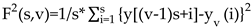
For . Here, is the fitting line in segment . Next, over all segments are averaged to obtain the -th order fluctuation function by
 where, the index variable can generally take any real value except zero. Repeating the above steps for several time scales, will increase as increases. The scaling behavior of the fluctuation functions could be analyzed by log-log plots versus for each value of . A power-law between and exists as the Eq. (5) when the series is long-range power-law correlated.

However, because of the diverging exponent, the averaging procedure of Eq. (4) could not be applied directly to calculate the value corresponds to the limit as . Instead, we must employ a logarithmic averaging procedure by Eq. (6).

The exponent generally depends on . For stationary series, is the well-defined Hurst exponent . So is called the generalized Hurst exponent. In a special case, when is independent from , it is defined as monofractal series. The distinct scaling patterns exhibited by small and large fluctuations have a substantial impact on the relationship between the -th order Hurst exponent and the scaling parameter . In the case of positive , segments characterized by a significant deviation from the expected trend, i.e., those with large variances, will exert a dominant influence on the average -order Hurst exponent . Consequently, a positive captures the scaling behavior of these segments with notable fluctuations, which typically correspond to smaller scaling exponents in multifractal time series. Conversely, for negative values, segments with smaller variances take precedence in determining the average -order Hurst exponent . Hence, a negative describes the scaling behavior of segments with minor fluctuations, which generally exhibit larger scaling exponents in multifractal time series. This intricate interplay between , the scaling behavior of different segments , and the corresponding fluctuations provides valuable insights into the multifractal nature of the time series, shedding light on how various levels of variance impact the overall scaling exponents.
The multifractal spectrum is another tool to characterize multifractality in a series. can be obtained by the Eq. (7)
 and then the Legendre transform

 where is the Holder exponent value which indicates the strength of singularity. When the is broader, it indicates a stronger multifractality or complexity.
The width of the spectrum could be
 where and indicate the maximum and minimum values respectively.
We name MF-DFA1, MFDFA2 and MFDFA3 separately with polynomial order . Here we apply MF-DFA1 and MF-DFA2 to investigate the BCTI, BDTI and specific routes of TC2 and TD7.
1.2. The Multifractal Detrending Moving Average Method
Following brief introduction of MF-DMA method is based on works of Gu and Zhou (2010) [41].
Assuming time series , and is the length of the series. We construct a new series
Next step, indicates the moving average function. To calculate the sequence of cumulative totals, we slide a window of fixed size across the sequence.
 where is the size of window, is the largest integer but not greater than , is the smallest integer but not smaller than , and is the position parameter, varying from 0 to 1. Here is calculated over data points from the preceding period while data points from the subsequent period. We have to notice three special cases with different values. The backward moving average, where and is calculated by all the past data points. refers to the centered moving average, where is calculated over half past and half future data points. means the forward moving average, where is based on the trend of future data points. In this context, we utilize the selected case , as it has demonstrated superior performance compared to the other two alternatives, based on evidence presented in references [37,41,43].
Subsequently, we eliminate the moving average component from the series to eliminate any underlying trend, resulting in a residual sequence .
 where .
Then, the residual series is divided into () non-overlapping segments, each of equal length . These segments can be represented as for, where . We can get the root-mean-square function by Eq. (14).
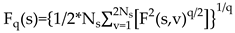
Additionally, the -th order overall fluctuation function is expressed as
Next step, when the values of varies, we can get the power-law relation between and in Eq. (17)

Finally, the multifractal scaling exponent and multifractal spectrum could be defined similarly with that of above MF-DFA.
1.3. The Effective Multifractality
According to the references [58,61], the total multifractal spectrum could be intricately divided into three parts: the non-linear and linear correlation, and the PDF. This decomposition is captured by the Eq. (18).

It is important to emphasize that both the linear correlation component and the nonlinear correlation component represent temporal correlations [2,5]. Specifically, the linear correlation component is attributed to finite-size effects [54,63]. Furthermore, it is noteworthy that indicating the linear correlation component, can be computed by semi-analytical formulas of an explicit form, offering a comprehensive quantitative characterization of this phenomenon [39]. A type of computational deviation stemming from the sample number constraints is defined as the finite-size effect in reference [26]. In essence, smaller time series sizes lead to greater computation deviations. To mitigate the impact of sample size limitations, especially for small sample sizes (<10000), it is necessary to calculate and exclude the linear correlation component from the true multifractality. Consequently, the true multifractality, denoted as , which encompasses the nonlinearity component , and the PDF component , is determined[40,59,61].
To depict the spectrum of multifractality, it is important to conduct an analysis that involves both the elimination of the linear correlation component stemming from the sample size limitations (sample size < 10000 points) and the decomposition of the remaining two effective parts [59,61,62]. This quantitative analysis can be achieved through the creation of two new series: the shuffled and the surrogated time series. The shuffled time series is generated through the shuffled original series. During the process, the temporal correlations are disrupted, while the probability distribution remains unaltered [43,61].
The creation of surrogate data is accomplished through a two-stage procedure. Initially, the process ensures that the surrogate data matches the original volatility time series in terms of probability distribution, which is executed through a transformation technique as described in reference [49]. Subsequently, the surrogate time series is manipulated to include linear correlations by applying an improved version of the amplitude-adjusted Fourier transform (IAAFT), as detailed in reference [59]. To gain a thorough grasp of the surrogate time series construction process, it is recommended that readers refer to the comprehensive explanation in the reference [26].
1.4. Machine Learning-Three Learners
Overall, we selected and combined three learners(XGBoost, LightBGM and CatBoost) from machine learning to form our stacking regression model. Therefore, the introduction of machine learning is based on three researches which are respectively done by Chen T , Guestrin C[54]; Ke G, Meng Q, Finley T[64]; Prokhorenkova L, Gusev G, Vorobev A[65].
XGBoost is a scalable tree boosting system, which firstly use tree boosting in a nutsheel to regularize learning objective:
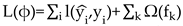 where , is the loss function, is the predicted value, is the target value, and are regularization parameters, is the number of trees, and represents the square of the output score on each tree's leaf nodes (equivalent to L2 regularization) .
Then, the system add ft to minimize objective and use second-order approximation to quickly optimize the objective in the general setting, the corresponding optimal is:
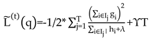
In the final stage, it is necessary to scale the newly added weights and perform column sampling to prevent overfitting (similar to random forests). XGBoost also includes a split finding algorithm, where the basic greedy algorithm enumerates all possible splits, calculates the gain for each split, and then selects the split with the maximum gain. The approximate algorithm, on the other hand, proposes candidate split points by mapping continuous features into bins and then aggregating statistics to find the optimal solution. In summary, XGBoost introduces a new sparse-aware algorithm and weighted quantile sketch, where caching access patterns, data compression, and partitioning are key, thus enabling the solution of real-world scale problems with minimal resources.
LightGBM is an efficient Gradient Boosting Decision Tree (GBDT) algorithm proposed by Ke et al. at the NIPS conference in 2017. It addresses the efficiency and scalability issues associated with high-dimensional features and large datasets by introducing two innovative techniques: Gradient-based One-Side Sampling (GOSS) and Exclusive Feature Bundling (EFB). The GOSS technique excludes data instances with small gradients, using only the remaining instances to estimate the information gain, thereby significantly reducing the amount of data processed while maintaining the accuracy of information gain estimation. The EFB technique reduces the number of features by bundling mutually exclusive features that rarely take non-zero values simultaneously, such as one-hot encoded features in text mining. LightGBM safely bundles these exclusive features together, constructing the same feature histograms from feature bundles as from individual features through a carefully designed feature scanning algorithm, thus reducing the complexity of histogram construction from O(#data×#feature) to O(#data×#bundle), where #bundle is much smaller than #feature, significantly accelerating the training of GBDT. Experimental results show that LightGBM is over 20 times faster in training on multiple public datasets while achieving nearly the same accuracy as traditional GBDT. These achievements not only demonstrate the superior performance of LightGBM in handling large-scale datasets but also provide new directions for the optimization of GBDT algorithms.
CatBoost introduced two algorithmic improvements: ordered boosting and an innovative algorithm for handling categorical features, corresponding to the Ordered mode and Plain mode (built-in ordered TS standard GBDT algorithm). For the Plain mode, multiple random permutations are first used to calculate gradients and TS, evaluate candidate splits, update the support model to construct decision trees, and then a complexity comparison and analysis with the standard GBDT algorithm is performed, culminating in the greedy construction of high-order feature combinations. CatBoost identified and analyzed the problem of prediction shift, proposing ordered boosting and ordered TS as solutions, and demonstrated superior performance in multiple benchmark tests.
1.5. Predictive Methodology Overview
To investigate how freight rates can help predict Brent oil prices in different periods, we employed the following methodology across four distinct periods (Period I-IV). In Table 1, each of these periods corresponds to a significant global event that profoundly affected both freight rates and oil prices.
For each of these periods, we employed the same predictive approach to understand the effect of multifractal features on forecasting oil prices. Specifically, the freight rates (BDTI) were utilized alongside different feature sets to predict Brent oil prices, with the following steps:
Direct Prediction Using BDTI: As a baseline, we predicted Brent prices using only BDTI data.
Addition of Crisis Period Indicator: We added an indicator for the crisis period to account for the impact of significant events (e.g., the financial crisis or the pandemic) on market dynamics.
Addition of Multifractal Features: Multifractal features extracted using the Multifractal Detrended Fluctuation Analysis (MFDFA) method were included to capture complex market behaviors.
Combination of Crisis Indicators and Multifractal Features: Both crisis indicators and multifractal features were included to examine their combined effect on prediction accuracy.
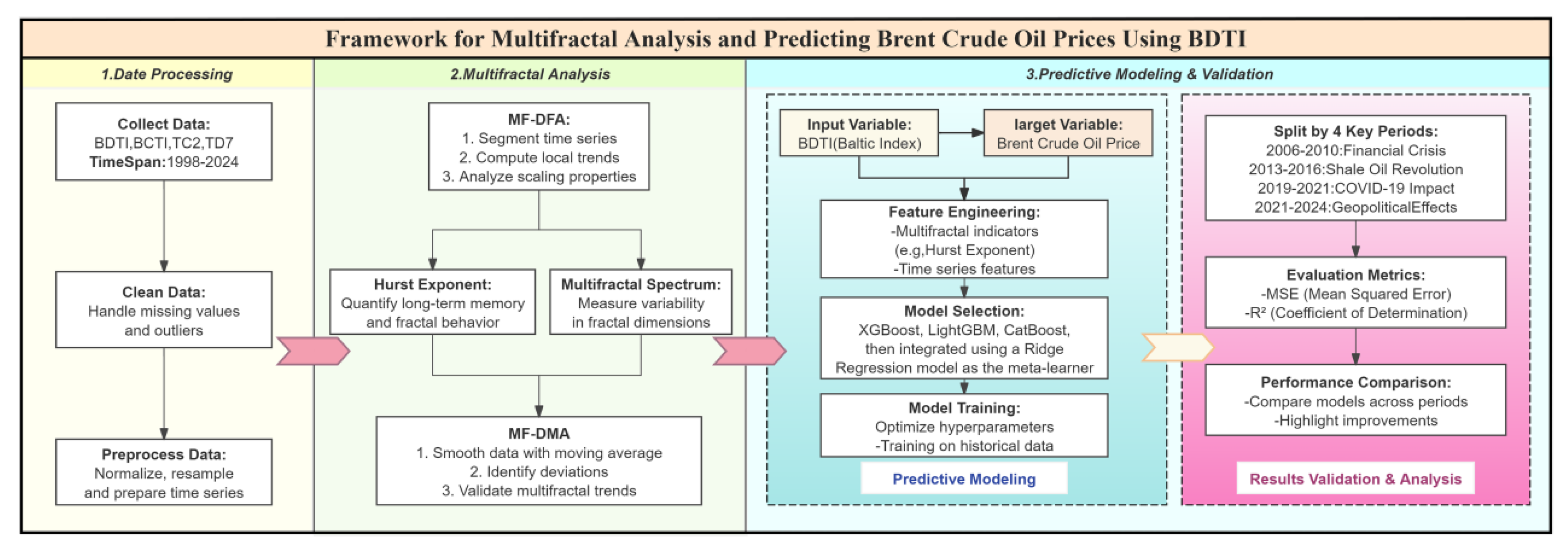
To provide a clear visual representation of the methodology, the following flowchart outlines the framework for multifractal analysis and predictive modeling using the Baltic Dirty Tanker Index (BDTI) and its application to Brent crude oil price prediction. This framework includes three key components: data processing, multifractal analysis, and predictive modeling and validation.
Figure 1.
Framework for Multifractal Analysis and Predictive Brent Crude Oil Prices Using BDTI. This visual representation complements the detailed methodology described above, offering readers an intuitive understanding of the step-by-step process adopted in this study, particularly how multifractal indicators and machine learning models are integrated for predictive modeling across the four structural break periods.
2. Data Description
The Baltic Clean Tanker Index (BCTI) is a widely tracked benchmark that measures the cost of shipping clean petroleum products, such as refined oil, on specific routes within the Baltic region [2,7,10,14]. It serves as a vital indicator for gauging freight rates and understanding the supply and demand dynamics within the clean tanker market. The BCTI's fluctuations influence various economic sectors, making it an essential tool for industry stakeholders, analysts, and investors seeking insights into energy market trends and shipping conditions. Therefore, we pay great attention to the BCTI and specific route of TC2 from Continent to USAC with clean tanker size of 37,000mt.
Similarly, The Baltic Dirty Tanker Index (BDTI) is a vital benchmark that assesses the cost of shipping dirty petroleum products, including crude oil, on selected routes within the Baltic region. It serves as a key indicator for understanding freight rates and evaluating the supply and demand dynamics within the dirty tanker market. A specific route of TD7 from North Sea to Continent with dirty tanker size of 80,000mt is selected to analyze.
The sample for daily BCTI and BDTI covers the period from Jan 28, 1998 to Jan 12, 2024. The sample size includes 6413 and 6358 points separately, which is enough for multifractal models [36,37,38,39,40,41]. However, the data for BCTI TC2 is 5014 points as the data begins from March 4, 2004. The data of BDTI TD7 includes 6234 points as we could not get the records for year 2023. The statistics results of sample time series are listed in Table 2. Figure 2 describes the BCTI and BDTI of the sample observations. There are big volatilities in the year 2008 under global financial crisis, in the year 2020 when the COVID-19 break out and in the year 2022 when geographic conflict happened. Figure 3 records the BCTI and BDTI logarithmic changes (that is ), which is widely applied to calculate daily volatilities and the returns often help to decrease non-stationarities though it is not required in multifractal methods [12,39].
3. Analysis of Results
3.1. Multifractality in Dirty and Clean Tanker Freight Rate Returns
The Hurst exponent is a measure that characterizes the rate at which the root-mean-square (RMS) deviation of a time series expands as the size of the observational window (i.e., the scale) grows, revealing the monofractal nature of the data [11,28,33,34,35]. In the context of a multifractal time series, the localized variations, or the RMS deviations, exhibit significantly large values for segments coinciding with periods of high fluctuation, and similarly, they show significantly small values for segments during periods of low fluctuation [32,33,34]. The q-order Hurst exponent is calculated by examining the slopes of the regression lines that relate the q-order RMS to the scale of the observation [36,37,38,39,40,41]. Figure 4(a) to (d) on the left illustrate that for multifractal time series, these slopes vary depending on the value of q. The distinction between the q-order RMS for positive and negative fluctuations is more pronounced at smaller segment widths than at larger ones. This is because smaller segments are more sensitive to the local variability within a specific period, whereas larger segments encompass multiple periods and tend to average out the differences in fluctuation magnitude. As q increases, the q-order RMS for a multifractal time series generally decreases, as shown on the right side of Figure 4(a) to (d). Both BCTI and BDTI returns exhibit multifractal characteristics, indicating that their fluctuation patterns are not uniform across different scales and require a more nuanced analysis to understand their underlying dynamics [12,43].
3.2. Multifractal Characteristics of Tanker Freight Fluctuation Under Structural Breaks
The logarithmic return of BCTI and BDTI and the specific routes in Figure 2 suggests that there exist big fluctuations in year 2008, year 2020 and year 2022 with events of financial crisis, COVID-19 and geographic conflict, which is in accordance with the references [7,9,12,46]. According to references, big events such as global financial crisis can lead to structural breaks in time series [45,47,48], we divide the sample data BDTI into two parts: period I from Jan 28, 1998 to Dec 01, 2010 and period II from Dec 02, 2010 to Jan 12, 2024 to delve into the changing external factors’ effects on the multifractalities.
The study of multifractal time series often involves various scaling exponents, among which the q-order Hurst exponent is prominent. However, the local Hurst exponent has proven advantageous in detecting specific time points of structural change within a time series [45,48,49,50], [58,59]. This local perspective aligns with q-order Hurst values for extreme fluctuations, correlating positively or negatively depending on the q value's sign. The utility of the local Hurst exponent is particularly evident when financial time series experience sudden disturbances. It pinpoints how these shocks modify the series' inherent scale-invariant features on a localized level [23,24,25,26,27]. Visualized through histograms, the temporal variations of the local Hurst exponent offer a probability distribution of these changes (illustrated in Figure 5 (e) for the first period and (f) for the second period). Complementing this, the multifractal spectrum – delineated by the parameters and captures the breadth of multifractality within the series (depicted in Figure 5 (e) for the first period and (f) for the second period). An increasing spectrum breadth denotes growing structural disparities between periods marked by minor and major fluctuations [25,26,27,28]. The research employs multifractal spectrum width as a measure of multifractality level, which, according to results presented in Figure 4 (e) and (f), confirms strong multifractality in both examined periods of the Baltic Dry Index (BDTI) returns. These findings align with previous research outlined in references [17,18], solidifying the observed characteristics of the market across different analytic methodologies. From Figure 5 (a) and (c), both the BCTI and BDTI markets are with multifractal characteristics though they are different from the specific routes of TC2 and TD7 in Figure 5 (b) and (d).
3.3. Temporal Dynamics of Tanker Freight Market Complexity with MF-DMA Method
In Figure 6 (a), the multifractality from PDF is , while the total multifractality from the three parts is . The multifractality from linear correlation and PDF are , so the multifractality from the non-linear correlation . The true multifractality. The results in Figure 6 (a)-(f) are listed in Table 3.
The multifractality analysis of the Baltic Clean Tankers market in Figure 6 (a) reveals significant insights into its dynamics. A multifractality value of 0.90 for the original data points to a highly complex market with pronounced multifractal behavior due to strong correlations at various time scales. A lesser, but still substantial, multifractality value of 0.61 in the surrogated data indicates that multifractality persists without temporal correlations, suggesting that price change distributions inherently contribute to market complexity. The shuffled data's multifractality value at 0.48, the lowest observed, illustrates the crucial role of temporal ordering in market behavior. These values collectively attest to the market's intricate and nonlinear interaction across scales [43].
The multifractality analysis for the Baltic Clean Tankers in Figure 6 (a) and (b), inclusive of the specific 37000 tonnage route, elucidates distinct market dynamics. The original data for the entire market and the targeted route yield high multifractality values of 0.9 and 0.86 respectively, underscoring considerable multifractal behavior. However, subsequent surrogated and shuffled data yield diminished multifractality values of 0.61 and 0.48 for the broader market, and 0.39 and 0.23 for the specific route, respectively. These reductions upon data modification suggest inherent temporal organization as a key contributor to multifractality [26,27,28,43]. The analysis underscores the influence of data structure on the assessment of market complexity and multifractal characteristics.
The multifractal analysis of the Baltic Dirty Tankers market data in Figure 6 (c) reveals varying degrees of market complexity. An original multifractality value of 0.58 indicates a moderate complex market structure with self-similarity across time scales. The surrogated data's 0.52 multifractality value suggests that nontrivial scaling behavior persists even after the removal of some structural correlations. This denotes inherent complexity within the price change distribution itself [14,26,27,28]. A notably lower multifractality value of 0.28 in the shuffled data emphasizes the importance of chronological order, indicating that temporal organization significantly contributes to the market’s multifractal nature [43].
The multifractal analysis for the Baltic Dirty Tankers market in a specific route TD7 at the 80000-tonnage level in Figure6 (d) exhibits a high degree of market complexity, with original data yielding a multifractality value of 1.03. This denotes a rich multifractal structure and extensive self-similarity across temporal scales. Upon surrogate treatment, multifractality is markedly reduced to 0.5, indicating a diminished multifractal behavior upon the exclusion of certain structural and temporal correlations. Further declines to a multifractality value of 0.28 in the shuffled data underscore the pivotal role of temporal sequencing in fostering multifractal properties.
3.4. Predictive Applications: Using BDTI to Predict Brent Oil Prices
3.4.1. Understanding a Complexity for the Specific Periods and Motivation for Predictive Modeling
The comparative assessment of the Baltic Dirty Tankers from the specified periods of 1998 to 2010 and 2010 to 2023 in Figure 6 (e) and (f) may provide valuable insights into the temporal changes in multifractal nature and complexity within the market dynamics. The original multifractality value of 0.72 in the first period decreases to 0.60, suggesting a potential reduction in complexity and multifractal behavior. For the period of 1998 to 2010, the surrogated data yields a multifractality value of 0.62, indicating a decrease in complexity compared to the original data; similar for the period from 2010 to 2023. The shuffled data provides additional insights into the temporal changes in multifractality [26,43]. For the period of 1998 to 2010, the shuffled data yields a multifractality value of 0.35, reflecting a notable reduction in complexity compared to the original and surrogated data. Likewise, for the period from 2010 to 2023, the value further decreases to 0.29, signaling a continued decrease in complexity during the later period. Overall, the period from 2010 to 2023 exhibits higher multifractality values across all data types, indicating stronger multifractal nature and greater complexity [16,26,27,28].
These findings prompted our interest in understanding the underlying driving factors behind this marked increase in market complexity post-2010. To gain deeper insights, we apply a novel predictive approach using freight rates (BDTI) to predict Brent oil prices during distinct periods, aiming to explore the predictive power of freight rates in different market phases.
Traditionally, most studies have focused on forecasting freight rates based on oil price movements, which aligns with the conventional economic logic that oil prices drive downstream costs, including shipping. However, freight rates can be highly responsive to immediate changes in supply-demand dynamics, vessel utilization rates, and macroeconomic shifts, making them potentially valuable indicators for predicting oil prices as well. Thus, in this study, we take an innovative stance by attempting to predict oil prices from freight rates, with the intention of providing additional insights and decision-making tools for governments, businesses, and individual investors, especially during periods of significant market volatility and complexity.
3.4.2. Case Study: Prediction for Period III (2019-01-01 - 2021-01-01)
The choice of Period III (2019-01-01 to 2021-01-01) as the initial focus for analysis does not carry any special significance. In this study, we consider all four structural break periods to be equally important. Thus, selecting any of them as the starting point for analysis would have been equally valid. Period III was simply chosen at random as the first period to examine.
The predictive process was performed using Baltic Dirty Tanker Index (BDTI) as the main feature, and the following additional features were systematically introduced to improve prediction performance:
Crisis Period Indicator: An indicator variable was introduced to capture the effect of the 2020 COVID-19 pandemic, particularly between December 2019 and June 2020. This indicator took the value of 1 during the crisis and 0 otherwise, to help the model account for the dramatic market shifts.
Multifractal Features: Multifractal characteristics of the BDTI time series were extracted using the MFDFA method. We computed the Hurst exponent for various q-values (ranging from -5 to 5) to quantify the complexity and self-similarity within the time series.
To combine these features for predicting Brent oil prices, we employed a stacking regression model, consisting of the following base learners:
XGBoost: Capable of handling high-dimensional feature spaces and mitigating overfitting, XGBoost was used with 300 estimators, a learning rate of 0.01, and a maximum depth of 3.
LightGBM: Known for its efficient handling of large datasets, LightGBM was configured similarly to XGBoost, to provide complementary strengths in feature learning.
CatBoost: Particularly effective in dealing with categorical features and reducing preprocessing requirements, CatBoost was employed with 300 iterations and a learning rate of 0.01.
The predictions from these base learners were then integrated using a Ridge Regression model as the meta-learner. This stacking approach allows the model to capture a diverse range of data patterns and interactions, improving the robustness of predictions.
The resulting predictions for Period III are illustrated in Figure 7, where multiple models are compared against the actual Brent oil prices. The models include:
Predicted_Direct: Predictions made using only the BDTI data.
Predicted_Time_Indicator: Incorporating the crisis time indicator to assess the effect of the COVID-19 pandemic.
Predicted_Multifractal: Including multifractal features derived from the BDTI to understand the impact of market complexity.
Predicted_Multifractal_Indicator: Utilizing both the crisis indicator and multifractal features to determine their combined influence.
While the Predicted_Direct model shows some deviations, particularly during major disruptions, the inclusion of multifractal features (Predicted_Multifractal) allows the model to better capture the intricate market dynamics, resulting in predictions that align more closely with the actual price trends. The Predicted_Multifractal_Indicator model demonstrates the best performance, especially during the high-volatility period in early 2020 when the COVID-19 pandemic caused a sharp drop in oil prices.
3.4.3. Predictive Results and Analysis for Period I - IV
Following the same methodology as applied in Period III, we conducted predictive modeling for Periods I, II, and IV, with the results summarized as follows:
Period I (2006-01-01 - 2010-12-31): The 2008 Global Financial Crisis had a profound effect on both freight rates and oil prices. Figure 8 shows the predictive results, indicating that the inclusion of multifractal features and crisis indicators significantly improved prediction accuracy compared to the direct approach.
Period II (2013-06-30 - 2016-06-30): During the 2014 Shale Oil Revolution, the predictive model that included multifractal features outperformed the direct prediction, as shown in Figure 9. The Predicted_Multifractal_Indicator model captured the complex fluctuations caused by shifts in the energy supply landscape more effectively.
Period IV (2021-01-01 - 2024-01-12): The 2022 Russia-Ukraine conflict introduced significant geopolitical uncertainty. Figure 10 illustrates that the Predicted_Multifractal_Indicator model again provided the best fit, with reduced error margins and greater alignment with actual price movements, highlighting the value of multifractal features during periods of high volatility.
3.4.4. Robustness Analysis of Prediction Methods
Above, we presented several intuitive figures that provide a visual comparison of the predictive performance of different models across the four periods. Now, we proceed to a more detailed quantitative analysis to corroborate these visual observations with empirical metrics. Specifically, we focus on the predictive accuracy as measured by the Mean Squared Error (MSE) and R² values, which offer critical insights into the effectiveness of incorporating multifractal features and crisis indicators into the forecasting models.
Figure 11 presents the Mean Squared Error (MSE) values for both the training and test sets across all periods, demonstrating the improvement in predictive accuracy after incorporating multifractal features. As shown in the figure, the inclusion of these features significantly reduces the MSE values across all four periods, with the greatest improvements observed in Periods II, III, and IV. This suggests that the predictive models benefited substantially from the added complexity of multifractal characteristics, especially in the post-2010 periods where market dynamics became increasingly intricate.
Figure 12 displays the R² scores for both the training and test sets, providing insights into the proportion of variance explained by the models. The predictive models with multifractal features exhibit substantially higher R² values compared to the direct prediction models. Specifically, for Periods II, III, and IV, the Predicted_Multifractal_Indicator model achieves R² values close to or exceeding 0.9, indicating a strong fit to the actual data. Interestingly, the enhancement in predictive performance is less pronounced for Period I, suggesting that the multifractal characteristics during this earlier period were less influential compared to the more recent periods. This aligns with our previous observations that post-2010 periods exhibited greater multifractality and complexity, thereby benefiting more from the incorporation of multifractal features.
To provide a more comprehensive understanding, Figure 13 illustrates the substantial percentage improvements in MSE and R² when multifractal features are incorporated into the predictive models for each period. For instance, during Period II, the R² for training improves by approximately 182.54%, and the R² for testing by 167.62%, highlighting a dramatic enhancement in model performance when multifractal features are added. Similarly, Period III shows an 88.60% improvement in training R² and a 117.14% increase in testing R², emphasizing the importance of capturing complex dynamics during high volatility phases, such as those triggered by the COVID-19 pandemic. Notably, the improvements in Periods II, III, and IV are significantly greater compared to Period I, which only shows modest gains, reinforcing the notion that market dynamics after 2010 became more intricate and multifaceted. This distinct difference in performance can be attributed to increased globalization, advancements in technology, and heightened geopolitical sensitivity after 2010, all contributing to more complex and unpredictable market interactions. These findings underscore that the multifractal characteristics are especially relevant for capturing the nuances of post-2010 market behavior, making the predictive models significantly more effective for later periods.
Such findings are critical, as they highlight the evolving nature of the oil market and underscore the importance of adapting predictive methodologies to account for changes in market structure and dynamics. The superior performance of models incorporating multifractal features during periods of heightened market complexity suggests that traditional linear models may be insufficient for capturing the nuanced behaviors of modern financial markets. By utilizing multifractal analysis, stakeholders can achieve a deeper understanding of market dynamics and enhance their decision-making processes, particularly during times of instability.
4. Discussion of Results
From the discussion, one may conclude that this study successfully unravels the multifaceted complexity of the Baltic Tanker Freight market using multifractal analysis techniques and advanced machine learning models. By integrating the Baltic Dirty Tanker Index (BDTI) as a leading indicator, we demonstrate that freight rates can effectively predict Brent oil prices, particularly during heightened market volatility caused by global crises such as the 2008 Financial Crisis, the 2014 Shale Oil Revolution, the COVID-19 pandemic, and the Russia-Ukraine conflict. The findings reveal that multifractal characteristics, such as the generalized Hurst exponent and multifractal spectrum, significantly enhance the predictive accuracy of the models, outperforming traditional approaches that rely solely on linear or unidirectional relationships [7,9]. Moreover, the stacking regression framework combining XGBoost, LightGBM, CatBoost, and Ridge Regression validates the robustness of the proposed methodology, aligning closely with contemporary machine learning advancements [26,62,63,64]. These results provide actionable insights for policymakers, energy companies, and investors, emphasizing the utility of multifractal analysis in managing systemic risks and navigating energy market volatility [4,6].
Comparison of the findings with those of other studies confirms the progressive advantage of integrating multifractal analysis with predictive modeling. Previous research has largely focused on forecasting freight rates based on oil prices, reflecting a conventional perspective of oil price-driven costs in shipping [17,18]. However, this study advances the discussion by demonstrating that BDTI provides valuable information for predicting Brent oil prices. This finding aligns with recent studies that highlight the sensitivity of freight rates to immediate supply-demand imbalances and macroeconomic shocks [74]. Unlike earlier studies that overlooked nonlinear dynamics, the inclusion of multifractal features offers a substantial improvement in capturing complex market behaviors. Thus, the predictive performance achieved in this study reflects methodological progress compared to traditional econometric models or linear approaches, which often fail under volatile conditions [12,18].
Nevertheless, there are limitations to the current study that warrant consideration. First, while the study leverages BDTI and multifractal features, it does not account for other exogenous factors such as regional economic policies, environmental regulations, or vessel fleet dynamics, which may further influence oil and freight markets [8]. Second, the analysis is constrained to the Baltic indices (BDTI and BCTI), which, although significant, may not fully represent global tanker market dynamics. Third, the use of historical data assumes that past patterns remain valid predictors for future trends, which may not hold during unprecedented disruptions or structural market changes [19,33]. Finally, the reliance on machine learning models, though effective, introduces the risk of overfitting, particularly when applied to smaller or less volatile datasets [51,52].
To address these limitations, several potential solutions can be proposed. Expanding the dataset to include additional variables such as global trade volumes, bunker fuel prices, or geopolitical risk indices may enhance the robustness of the models [19,21]. Incorporating real-time data streams or satellite-based tracking of vessel movements could also improve predictive accuracy [52,53]. Furthermore, the application of hybrid methods, combining deep learning approaches like Long Short-Term Memory (LSTM) networks with multifractal analysis, could address the limitations of traditional machine learning models.
Research questions that could be asked include whether integrating additional market indicators, such as energy derivatives or macroeconomic indicators, could further refine predictive outcomes [14]. One important future direction of this research is to explore the interplay between multifractality and emerging market phenomena, such as carbon emissions trading and the adoption of alternative fuels in shipping. Moreover, investigating the applicability of multifractal analysis in other energy markets, such as natural gas or LNG freight rates, may provide deeper insights into the broader dynamics of energy transportation [16,19]. These experimental research results will hopefully serve as useful feedback information for future iterations of predictive frameworks.
In conclusion, this study demonstrates the significant potential of multifractal analysis and machine learning in accurately forecasting energy prices during periods of high volatility. The findings not only advance the theoretical understanding of tanker freight markets but also provide practical tools for stakeholders to manage uncertainty and enhance decision-making. By successfully integrating multifractal features and advanced predictive models, this study offers a robust framework that can serve as a foundation for future research. Moving forward, further refinements and broader applications of the proposed methodology may uncover additional insights into the intricate relationships shaping global energy markets, paving the way for more resilient and adaptive forecasting strategies.
5. Conclusions
This study utilizes MF-DMA methodology to unravel the multifaceted nature of the Baltic Tanker freight market. Initial findings suggest an overarching multifractal nature within the market, with total multifractality reaching up to 0.90 in the Clean Tankers market. This complexity arises partly from a fat-tailed probability distribution (0.48) and non-linear correlations (0.29), indicating sophisticated temporal organization and inherent volatility as core components of market behavior. A closer examination of a specific route (TC2, 37,000-tonnage) shows that the market retains its multifractal attributes, albeit with reduced magnitudes upon data manipulation. This consistent reduction in multifractality values—evident upon shuffling and surrogating—reinforces the significant contribution of temporal arrangement to the market's complex structure. The world clean tanker market reflects a tight supply-demand balance, with freight rates fluctuating significantly in response to external changes.
In the case of the Dirty Tankers market, the study highlights moderate complexity, with an original multifractality value of 0.58, diminishing under surrogate and shuffled scenarios. This suggests that chronological sequencing is crucial for preserving multifractal properties in this segment. This assertion is further substantiated by focusing on specific routes like TD7 (80,000-tonnage), where multifractality peaks at 1.03 but declines markedly when temporal and structural correlations are disrupted.
The transition in multifractal dynamics between 1998–2010 and 2010–2024 reflects a shift from crisis-induced market behaviors to diversified and complex dynamics influenced by technological advancements, regulatory changes, and environmental policies.
Building on these findings, the study proposes a novel predictive framework that integrates the Baltic Dirty Tanker Index (BDTI), multifractal features, and crisis period indicators to forecast Brent oil prices during periods of heightened volatility. An analysis of four major global events—the 2008 Financial Crisis, the 2014 Shale Oil Revolution, the COVID-19 pandemic, and the Russia-Ukraine conflict—illustrates how external factors influence market dynamics and energy prices. The advanced machine learning models employed, including stacking regression with XGBoost, LightGBM, CatBoost, and Ridge Regression, enhance the robustness and reliability of predictions. These methods highlight the potential of freight rates as leading indicators for energy markets, providing actionable insights for policymakers and market participants.
In conclusion, this study combines multifractal analysis and predictive modeling to provide a comprehensive framework for understanding and navigating the complexities of the Baltic Tanker freight market. By revealing the evolving multifractal dynamics and demonstrating the predictive power of freight rates, the research underscores the importance of integrating multifractal characteristics into forecasting models. The findings offer practical implications for strategic decision-making, operational resilience, and risk management in the shipping and energy industries. Future studies should build on this framework by incorporating additional datasets, refining predictive algorithms, and exploring the interplay between multifractality and other market indicators to further enhance prediction accuracy and application scope.
Author Contributions
Conceptualization, F.C., H.J. and X.L.; methodology, Y.S.; software, F.C. and Y.S.; validation, F.C. and Y.S.; formal analysis, Y.S.; investigation, H.J. and K.P.; resources, X.L.; data curation, X.L.; writing—original draft preparation, Y.S., H.J. and K.P.; writing—review and editing, F.C. and X.L.; visualization, X.L.; supervision, F.C. and X.L.; project administration, X.L.; funding acquisition, F.C. All authors have read and agreed to the published version of the manuscript.
Funding
The National Social Science Fund of China (No. 23BJL020) supports our research.
Data Availability and Conflict of Interest Statement
The data that support the findings of this study are available from the third party named Clarksons (https://sin.clarksons.net/), but restrictions apply to the availability of these data, which were used under licenses for the current study and so are not publicly available.
Competing Interests
No: I declare that the authors have no competing interests as defined by Springer, or other interests that might be perceived to influence the results and/or discussion reported in this paper.
Declaration of generative AI and AI-assisted technologies in the writing process
During the preparation of this work the author(s) used Doubao in order to improve language and readability. After using this tool/service, the author(s) reviewed and edited the content as needed and take(s) full responsibility for the content of the publication.
References
- Adland, R.; Cullinane, K. The non-linear dynamics of spot freight rates in tanker markets. Transportation Research Part E: Logistics and Transportation Review. 2006, 42, 211–224. [Google Scholar] [CrossRef]
- Zhang, J.; Zeng, Q. Modelling the volatility of the tanker freight market based on improved empirical mode decomposition. Applied Economics. 2017, 1223823. [Google Scholar] [CrossRef]
- Sun, X.; Haralambides, H.; Liu, H. Dynamic spillover effects among derivative markets in tanker shipping. Transportation Research Part E: Logistics and Transportation Review. 2019, 122, 384–409. [Google Scholar] [CrossRef]
- Gao, Y.; Zhang, L. The Impact of Geopolitical Events on Oil Market Dynamics: A Multifractal Analysis. Energy Economics 2017, 64, 48–56. [Google Scholar]
- Monge, M.; Romero Rojo, M.F.; Gil-Alana, L.A. The impact of geopolitical risk on the behavior of oil prices and freight rates. Energy. 2023, 269, 126779. [Google Scholar] [CrossRef]
- Zhang, Z.; Wang, Y.; Xiao, J.; Zhang, Y. Not all geopolitical shocks are alike: Identifying price dynamics in the crude oil market under tensions. Resources Policy. 2023, 80, 103238. [Google Scholar] [CrossRef]
- Khan, K.; Su, C.W.; Tao, R.; Umar, M. How often do oil prices and tanker freight rates depend on global uncertainty? Regional Studies in Marine Science. 2021, 48, 102043. [Google Scholar] [CrossRef]
- Cheong, S.S.; Kim, Y.D. The Impact of Environmental Regulations on the Shipping Industry: A Review. Sustainability 2019, 11, 371. [Google Scholar]
- Chen, J.; Zhao, R.; Xiong, W.; Wan, Z.; Xu, L.; Zhang, W. Influencing factors of crude oil maritime shipping freight fluctuations: A case of Suezmax tankers in Europe–Africa routes. Maritime Business Review. 2023, 8, 48–64. [Google Scholar] [CrossRef]
- Bai, X. Tanker freight rates and economic policy uncertainty: A wavelet-based copula approach. Energy. 2021, 235, 121383. [Google Scholar] [CrossRef]
- Abouarghoub, W.; Nomikos, N.K.; Petropoulos, F. On reconciling macro and micro energy transport forecasts for strategic decision making in the tanker industry. Transportation Research Part E: Logistics and Transportation Review. 2018, 113, 225–238. [Google Scholar] [CrossRef]
- Chen, F.; Miao, Y.; Tian, K.; Ding, X.; Li, T. Multifractal cross-correlations between crude oil and tanker freight rate. Physica A 2017, 474, 344–354. [Google Scholar] [CrossRef]
- Michail, N.A.; Melas, K.D. Quantifying the relationship between seaborne trade and shipping freight rates: A Bayesian vector autoregressive approach. Maritime Transport Research. 2020, 1, 100001. [Google Scholar] [CrossRef]
- Gavriilidis, K.; Kambouroudis, D.S.; Tsakou, K.; Tsouknidis, D.A. Volatility forecasting across tanker freight rates: The role of oil price shocks. Transportation Research Part E: Logistics and Transportation Review. 2018, 118, 376–391. [Google Scholar] [CrossRef]
- Regli, F.; Nomikos, N.K. The eye in the sky – Freight rate effects of tanker supply. Transportation Research Part E. 2019, 125, 402–424. [Google Scholar] [CrossRef]
- Gavalas, D.; Syriopoulos, T.; Tsatsaronis, M. COVID–19 impact on the shipping industry: An event study approach. Transport Policy. 2022, 116, 157–164. [Google Scholar] [CrossRef]
- Shi, W.; Li, K.X.; Yang, Z.; Wang, G. Time-varying copula models in the shipping derivatives market. Empirical Economics. 2017. [Google Scholar] [CrossRef]
- Siddiqui, A.W.; Basu, R. An empirical analysis of relationships between cyclical components of oil price and tanker freight rates. Energy. 2020, 200, 117494. [Google Scholar] [CrossRef]
- Bai, X.; Lam JS, L. Freight rate co-movement and risk spillovers in the product tanker shipping market: A copula analysis. Transportation Research Part E: Logistics and Transportation Review. 2021, 149, 102315. [Google Scholar] [CrossRef]
- Zhang, X.; Podobnik, B.; Kenett, D.Y.; Stanley, H.E. Systhmic Risk and Causality Dynamics of the World International Shipping Market. Physic A. 2014, 415, 43–53. [Google Scholar] [CrossRef]
- Khan, K.; Su, C.W.; Khurshid, A.; Umar, M. The dynamic interaction between COVID-19 and shipping freight rates: A quantile on quantile analysis. European Transport Research Review. 2022, 14, 1–16. [Google Scholar] [CrossRef] [PubMed]
- Mantegna, R.N.; Stanley, H.E. Scaling behaviour in the dynamics of an economic index. Nature. 1995, 376, 46–49. [Google Scholar] [CrossRef]
- Mantegna, R.N.; Stanley, H.E. An Introduction to Econophysics, Cambridge University Press, Cambridge. 1999.
- Bouchaud, J.P.; Potters, M. Theory of Financial Risk, Cambridge University Press, Cambridge. 2000.
- Drożdż, S.; Kwapień, J.; Oświecimka, P.; Rak, R. Quantitative features of multifractal subtleties in time series. Europhys. Lett. 2009, 88, 60003. [Google Scholar] [CrossRef]
- Zhou, W.-X. Finite-size effect and the components of multifractality in financial volatility. Chaos, Solitons & Fractals 2012, 45, 147–155. [Google Scholar] [CrossRef]
- Di Matteo, A.; Pirrotta, A. Generalized differential transform method for nonlinear boundary value problem of fractional order. Communications in Nonlinear Science and Numerical Simulation. 2015, 29, 88–101. [Google Scholar] [CrossRef]
- Grech, D. Chaos, Alternative measure of multifractal content and its application in finance. Solitons & Fractals 2016, 88, 183–195. [Google Scholar] [CrossRef]
- Mandelbrot, B.B. The Fractal Geometry of Nature, Freeman, New York. 1982.
- Mantegna, R.N.; Stanley, H.E. Turbulence and Financial Markets. Nature. 1996, 383, 587–588. [Google Scholar] [CrossRef]
- Hurst, H.E.; Black, R.P.; Simaika, Y.M. Long-Term Storage: An Experimental Study, Constable, London. 1965.
- Castro e Silva, J.G. Moreira, Roughness exponents to calculate multi-affine fractal exponents. Physica A. 1997, 235, 327. [Google Scholar] [CrossRef]
- Peng, C.K.; Havlin, S.; Stanley, H.E.; Goldberger, A.L. Quantification of scaling exponents and crossover phenomena in nonstationary heartbeat time series. Chaos. 1995, 5, 82–87. [Google Scholar] [CrossRef]
- Kantelhardt, J.W.; Zschiegner, S.A.; Koscielny-Bundec, E.; Havlind, S.; Bunde, A.; Stanley, H.E. Multifractal detrended fluctuation analysis of nonstationary time series. Physica A 2002, 316, 87–114. [Google Scholar] [CrossRef]
- Yamasaki, K.; Muchnik, L.; Havlin, S.; Bunde, A.; Stanley, H.E. Scaling and memory in volatility return intervals in financial markets. Proc Natl Acad Sci U S A 2005, 102, 9424–9428. [Google Scholar] [CrossRef] [PubMed]
- Ihlen, E.A. Introduction to multifractal detrended fluctuation analysis in matlab. Front Physiol. 2012, 3, 00141. [Google Scholar] [CrossRef] [PubMed]
- Green, E.; Hanan, W.; Heffernan, D. The origins of multifractality in financial time series and the effect of extreme events. The European Physical Journal B 2014, 87, 1–9. [Google Scholar] [CrossRef]
- Grech, D.; Czarnecki, L. Multifractal dynamics of stock markets. Acta Phys. Polon. A. 2010, 117, 623–629. [Google Scholar] [CrossRef]
- Grech, D.; Pamuła, G. On the multifractal effects generated by monofractal signals. Physica A: Statistical Mechanics and its Applications 2013, 392, 5845–5864. [Google Scholar] [CrossRef]
- Arianos, S.; Carbone, A. Detrending moving average algorithm: A closed-form approximation of the scaling law. Physica A: Statistical Mechanics and its Applications 2007, 382, 9–15. [Google Scholar] [CrossRef]
- Gu, G.F.; Zhou, W.X. Detrending moving average algorithm for multifractals. Physical Review E 2010, 82, 011136. [Google Scholar] [CrossRef]
- Stanley, H.E.; Gabaix, X.; Gopikrishnan, P.; Plerou, V. Economic Fluctuations and Statistical Physics: The Puzzle of Large Fluctuations. Nonlinear Dynamics. 2006, 44, 329–340. [Google Scholar] [CrossRef]
- Kwapień, J.; Blasiak, P.; Drożdż, S.; Oświȩcimka, P. Genuine multifractality in time series is due to temporal correlations. Physical Review E. 2023, 107, 034139. [Google Scholar] [CrossRef]
- Zhang, Y. Investigating dependencies among oil price and tanker market variables by copula-based multivariate models. Energy. 2018, 161, 435–446. [Google Scholar] [CrossRef]
- Chen, F.; Tian, K.; Ding, X.; Li, T.; Miao, Y.; Lu, C. Multifractal characteristics in maritime economics volatility. International Journal of Transport Economics. 2017, 44. [Google Scholar] [CrossRef]
- Li, Y.; Yin, M.; Khan, K.; Su, C.W. The impact of COVID-19 on shipping freights: Asymmetric multifractality analysis. Maritime Policy and Management. 2023, 50, 2081372. [Google Scholar] [CrossRef]
- Buonocore, R.J.; Aste, T.; Di Matteo, T. Measuring multiscaling in financial time-series. Chaos, Solitons and Fractals. 2016. [CrossRef]
- Vogl, M. Controversy in financial chaos research and nonlinear dynamics: A short literature review. Chaos, Solitons and Fractals. 2022, 162, 112444. [Google Scholar] [CrossRef]
- Press, W.H.; Teukolsky, S.A.; Vetterling, W.T.; Flannery, B.P. Numerical recipes in FORTRAN: The art of scientific computing. Cambridge: Cambridge University Press.1996.
- Grobys, K. A multifractal model of asset (in)variances. Journal of International Financial Markets, Institutions and Money. 2023, 85. [Google Scholar] [CrossRef]
- Chen, T.; Guestrin, C. XGBoost: A Scalable Tree Boosting System. Proceedings of the 22nd ACM SIGKDD International Conference on Knowledge Discovery and Data Mining, 2016, 785-794.
- Ke, G.; Meng, Q.; Finley, T.; et al. LightGBM: A Highly Efficient Gradient Boosting Decision Tree. Advances in Neural Information Processing Systems 2017, 30, 3146–3154. [Google Scholar]
- Prokhorenkova, L.; Gusev, G.; Vorobev, A.; Dorogush, A.V.; Gulin, A. CatBoost: Unbiased Boosting with Categorical Features. Advances in Neural Information Processing Systems. 2018, 31, 6638–6648. [Google Scholar]
- Chen, T.; Guestrin, C. Xgboost: A scalable tree boosting system[C]//Proceedings of the 22nd acm sigkdd international conference on knowledge discovery and data mining. 2016: 785-794.
- Chen, F.; Miao, Y.; Tian, K.; Ding, X.; Li, T. Multifractal cross-correlations between crude oil and tanker freight rate. Physica A: Statistical Mechanics and its Applications 2017, 474, 344–354. [Google Scholar] [CrossRef]
- Li, T.; Xue, L.; Chen, Y.; Chen, F.; Miao, Y.; Shao, X.; Zhang, C. Insights from multifractality analysis of tanker freight market volatility with common external factor of crude oil price. Physica A: Statistical Mechanics and its Applications 2018, 505, 374–384. [Google Scholar] [CrossRef]
- Chen, F.; Yin, S.; Zhang, J.; et al. The interplay between multifractal characteristics and seasonal fluctuations within the LNG spot freight market: Insights, forecasting, and trading strategies. Nonlinear Dyn 2024. [Google Scholar] [CrossRef]
- Halsey, T.C.; Jensen, M.H.; Kadanoff, L.P.; Procaccia, I.; Shraiman, B.I. Fractal measures and their singularities: The characterization of strange sets. Phys Rev A. 1986, 33, 1141–1151. [Google Scholar] [CrossRef]
- Schumann, A.Y.; Kantelhardt, J.W. Multifractal moving average analysis and test of multifractal model with tuned correlations. Physica A. 2011, 390, 2637–2654. [Google Scholar] [CrossRef]
- Li, Q.; Fu, Z.; Yuan, N.; Xie, F. Effects of non-stationarity on the magnitude and sign scaling in the multi-scale vertical velocity increment. Physica A: Statistical Mechanics and its Applications. 2014, 410, 9–16. [Google Scholar] [CrossRef]
- Zhou, W.-X. The components of empirical multifractality in financial returns. Europhysics Letters 2009, 88, 28004. [Google Scholar] [CrossRef]
- Jiang, Z.Q.; Xie, W.J.; Zhou, W.X.; Sornette, D. Multifractal analysis of financial markets: A review. In Reports on Progress in Physics. 2019, 82, 125901. [Google Scholar] [CrossRef]
- Rak, R.; Grech, D. Quantitative approach to multifractality induced by correlations and broad distribution of data. Physica A: Statistical Mechanics and Its Applications. 2018, 508, 48–66. [Google Scholar] [CrossRef]
- Ke, G.; Meng, Q.; Finley, T.; et al. Lightgbm: A highly efficient gradient boosting decision tree. Advances in neural information processing systems 2017, 30. [Google Scholar]
- Prokhorenkova, L.; Gusev, G.; Vorobev, A.; et al. CatBoost: Unbiased boosting with categorical features. Advances in neural information processing systems 2018, 31. [Google Scholar]
- Zhang, X.; Bao, Z.; Ge, Y.E. Investigating the determinants of shipowners’ emission abatement solutions for newbuilding vessels. Transportation Research Part D: Transport and Environment. 2021, 99, 102989. [Google Scholar] [CrossRef]
- Schreiber, T.; Schmitz, A. Improved surrogate data for nonlinearity tests. Phys Rev Lett; 1996, 77, 635–638. [Google Scholar] [CrossRef]
- Morales Martínez, J.L.; Segovia-Domínguez, I.; Rodríguez, I.Q.; Horta-Rangel, F.A.; Sosa-Gómez, G. A modified Multifractal Detrended Fluctuation Analysis (MFDFA) approach for multifractal analysis of precipitation. Physica A: Statistical Mechanics and its Applications. 2021, 565, 125611. [Google Scholar] [CrossRef]
- Doğan, B.; Driha, O.M.; Balsalobre Lorente, D.; Shahzad, U. The mitigating effects of economic complexity and renewable energy on carbon emissions in developed countries. Sustainable Development. 2021, 29, 1–12. [Google Scholar] [CrossRef]
- Yang, M.; Lam, J.S.L. Operational and economic evaluation of ammonia bunkering – Bunkering supply chain perspective. Transportation Research Part D: Transport and Environment. 2023, 117, 103666. [Google Scholar] [CrossRef]
- Xie, W.J.; Wei, N.; Zhou, W.X. An interpretable machine-learned model for international oil trade network. 2023, 3, 103513. [CrossRef]
- Xue, L.; Chen, F.; Fu, G.; Xia, Q.; Du, L. Stability Analysis of the World Energy Trade Structure by Multiscale Embedding. Frontiers in Energy Research. 2021, 9, 729690. [Google Scholar] [CrossRef]
- Meza, A.; Koç, M. The LNG trade between Qatar and East Asia: Potential impacts of unconventional energy resources on the LNG sector and Qatar’s economic development goals. Resources Policy. 2021, 70, 101886. [Google Scholar] [CrossRef]
- Hu, W.; Zhang, X.; Wang, Y.; Chen, Z. Forecasting crude oil prices using reservoir computing models. Energy Economics 2024, 135, 106712. [Google Scholar] [CrossRef]
Figure 2.
Baltic Clean and Dirty Tanker Freight Rate Index.
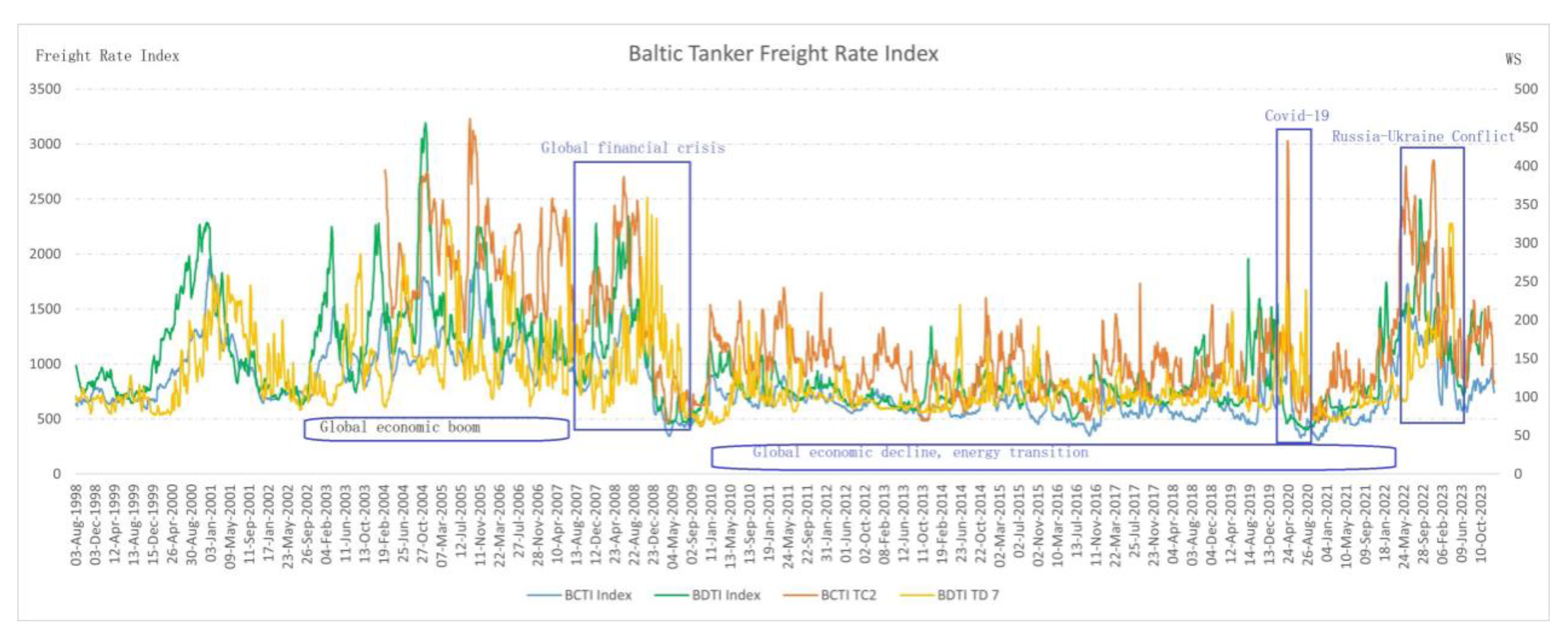
Figure 3.
Logarithmic Return of BCTI and BDTI.
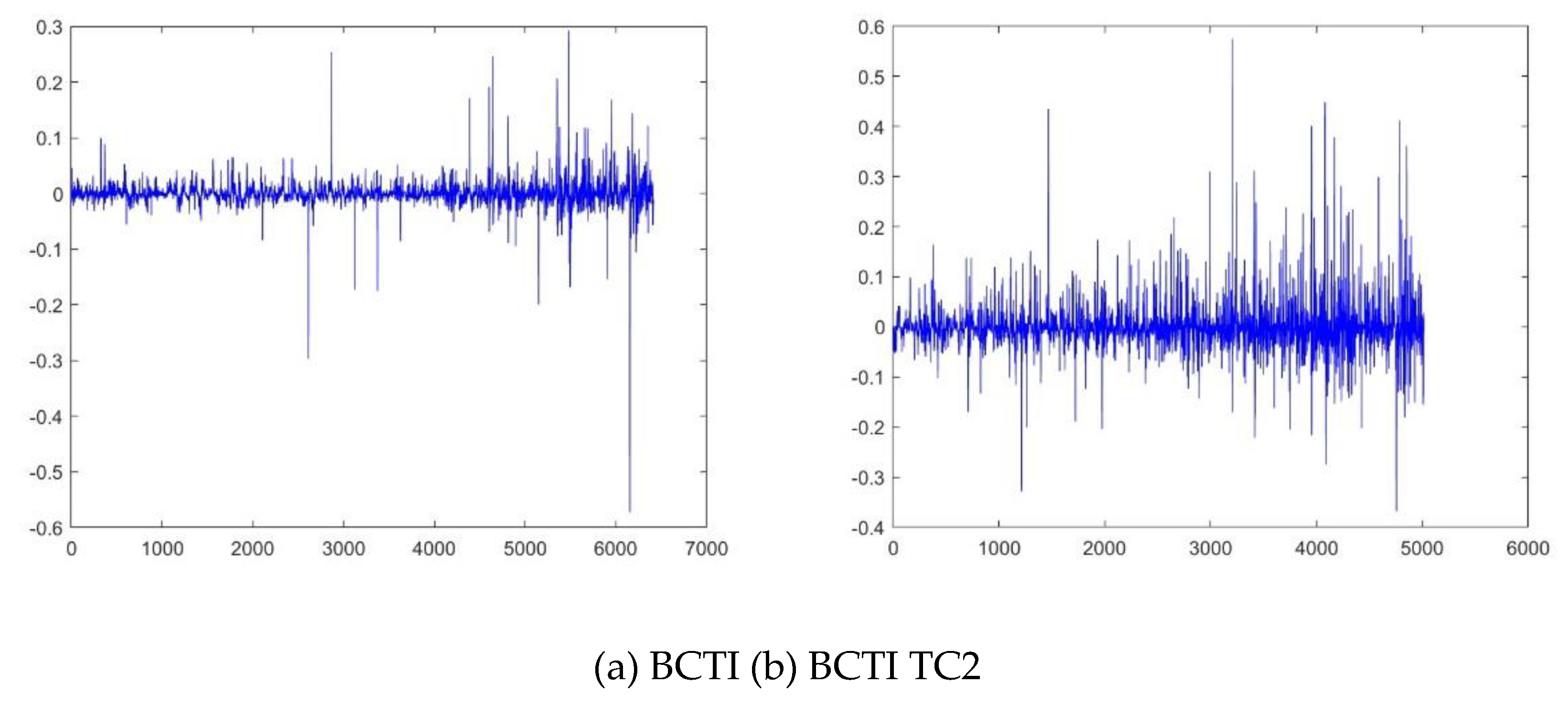
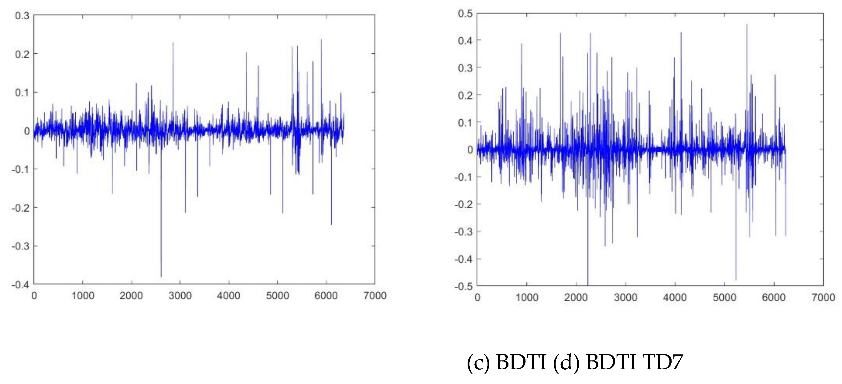
Figure 4.
Scaling function and Hurst exponent for BCTI return and BDTI return.
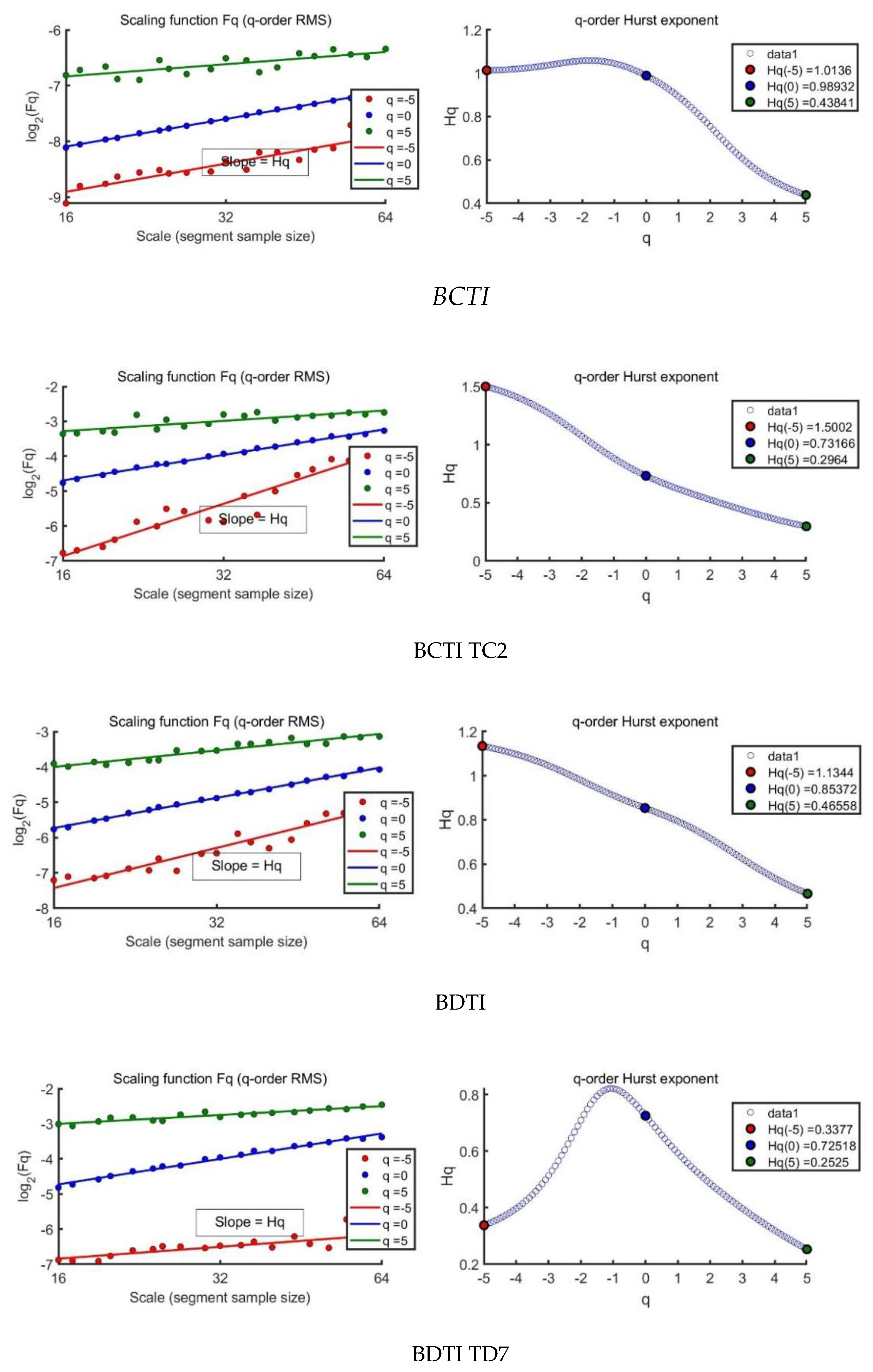
Figure 5.
Multifractal analysis of BCTI and BDTI return by MF-DFA2.
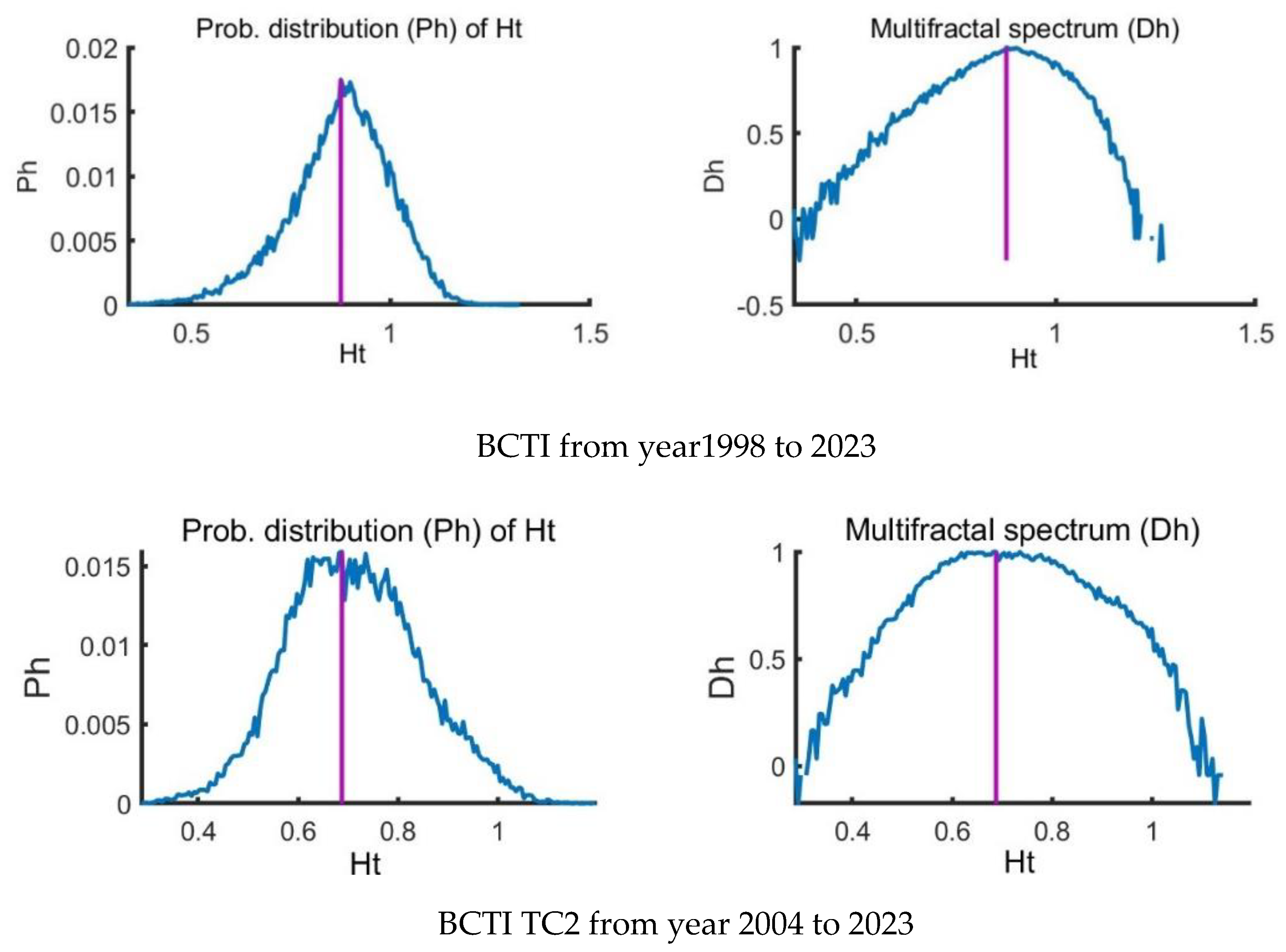
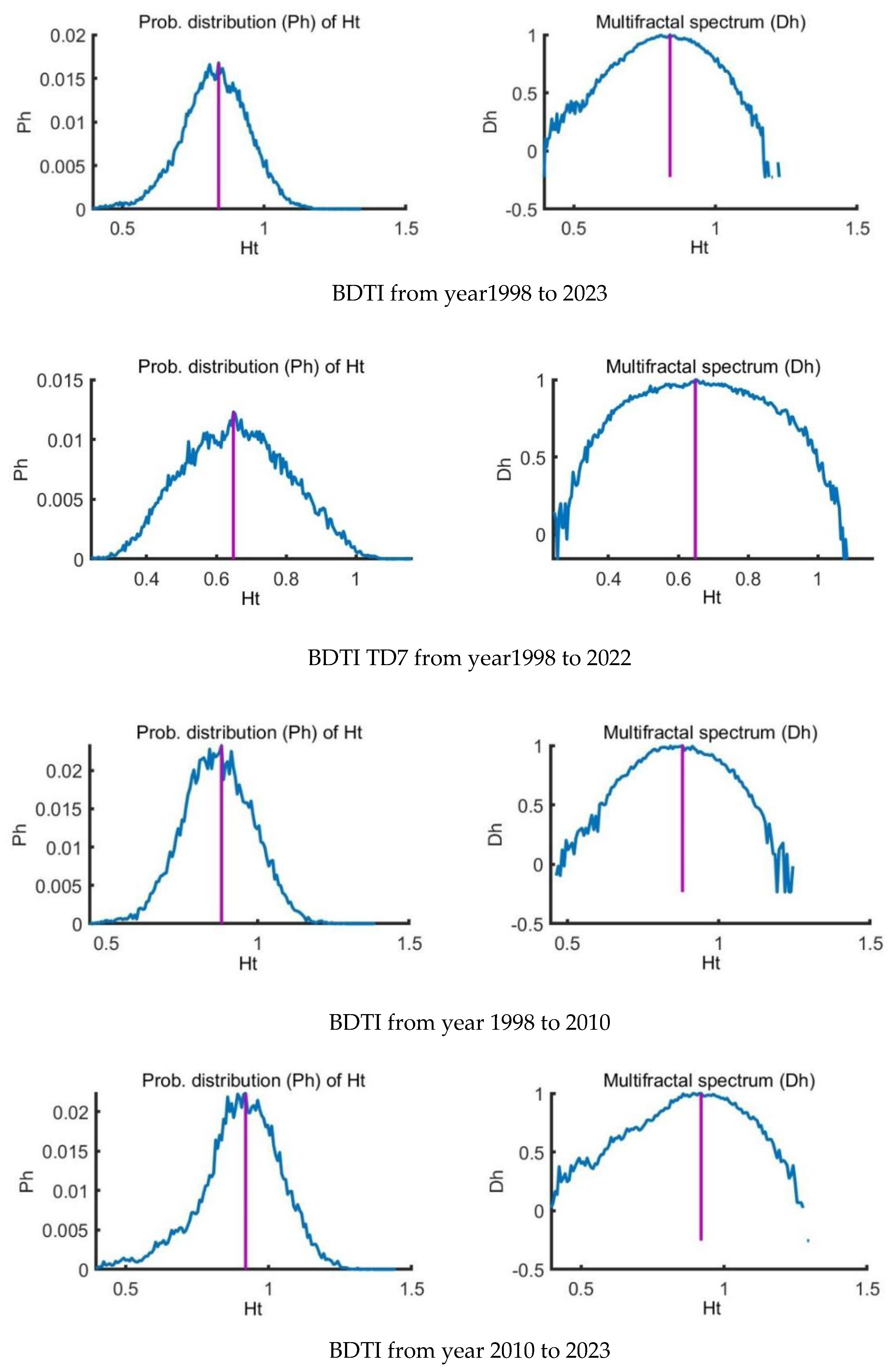
Figure 6.
The tanker freight rate’s multifractal sources by MF-DMA.
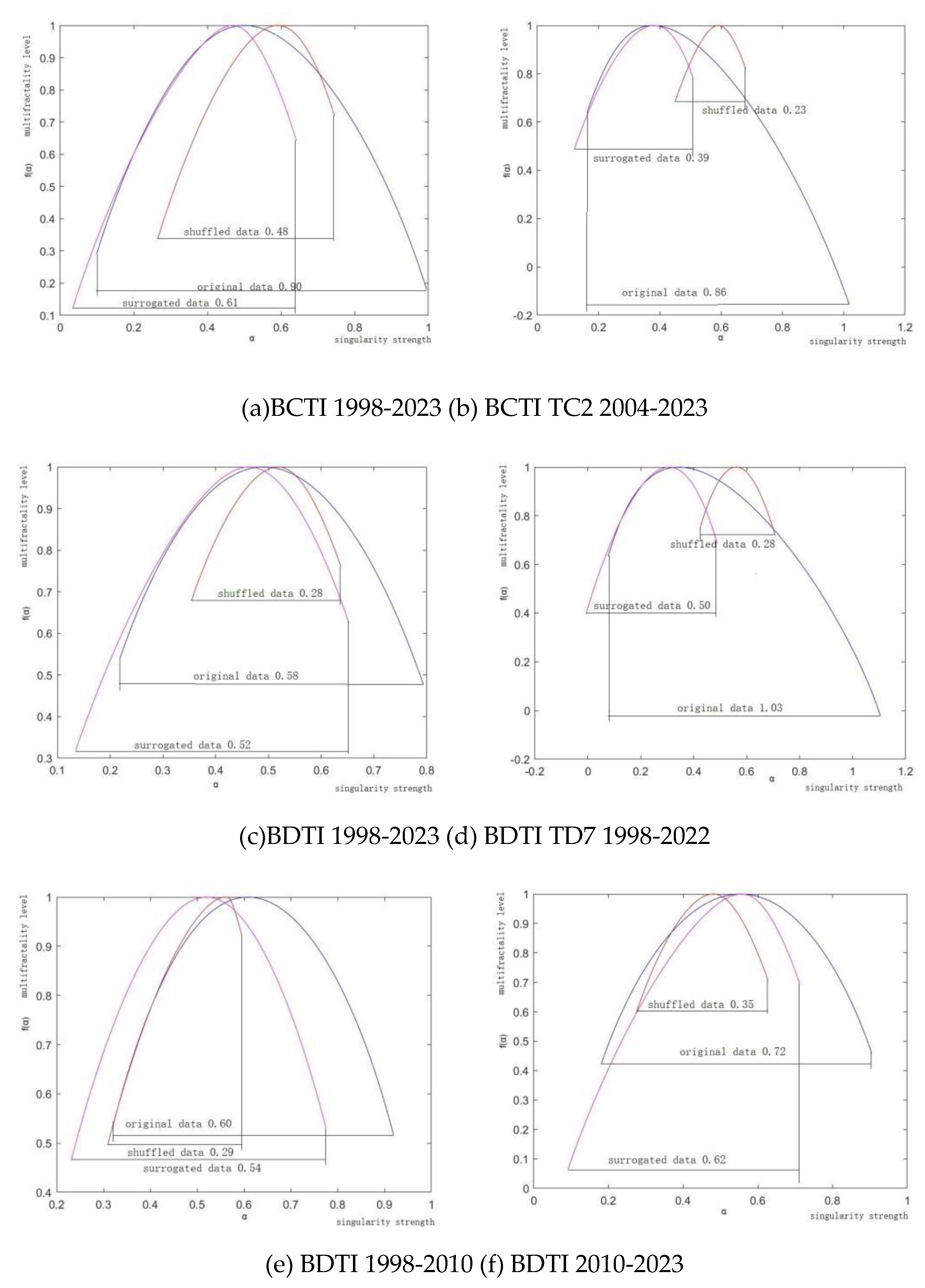
Figure 7.
Predictive Results for Brent Oil Prices during Period III (2019-01-01 to 2021-01-01) Using Various Models. It is evident that incorporating the crisis period indicator and multifractal features significantly enhances the model's prediction accuracy for Period III.
Figure 7.
Predictive Results for Brent Oil Prices during Period III (2019-01-01 to 2021-01-01) Using Various Models. It is evident that incorporating the crisis period indicator and multifractal features significantly enhances the model's prediction accuracy for Period III.
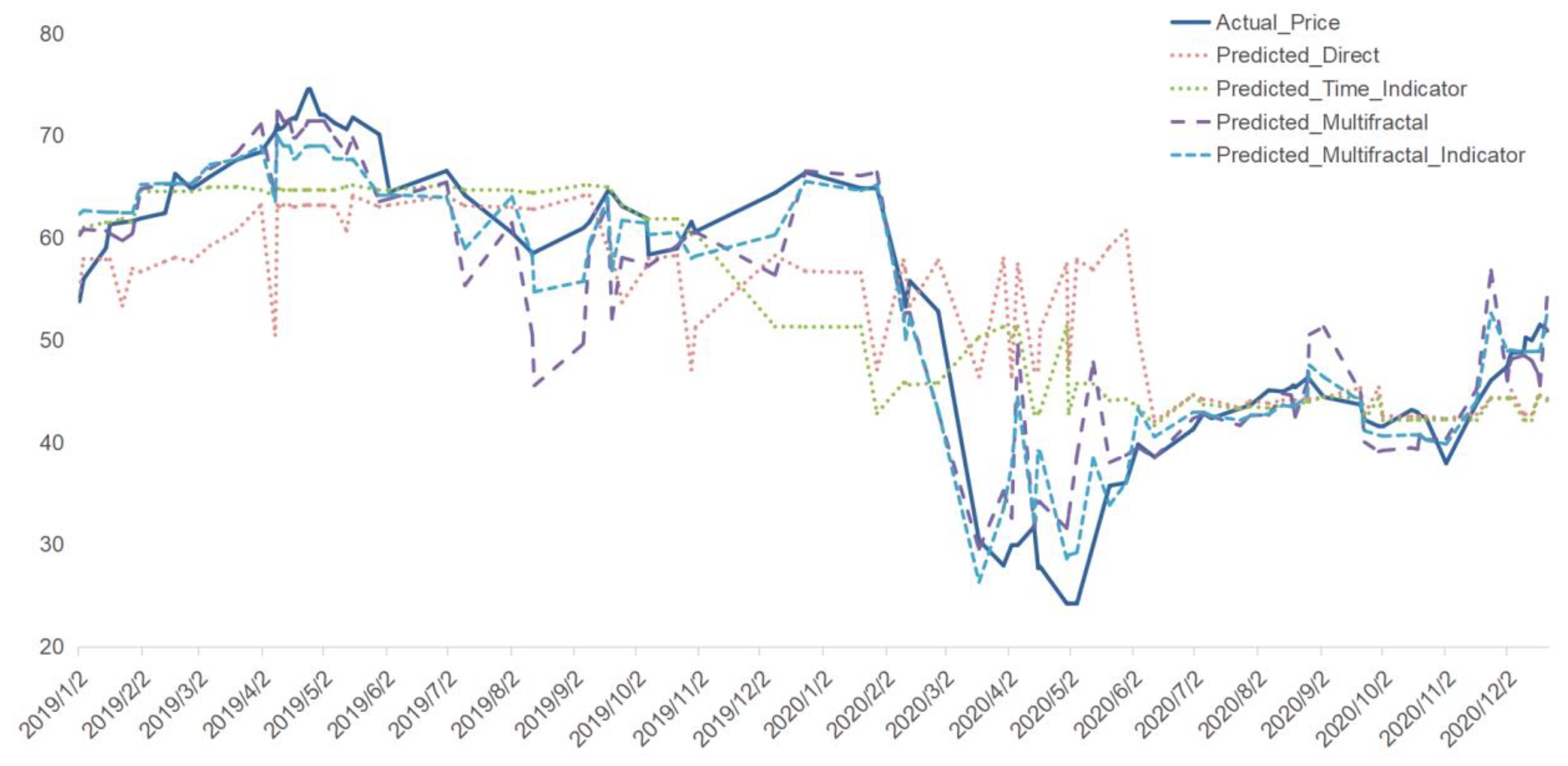
Figure 8.
Predictive Results for Brent Oil Prices during Period I.
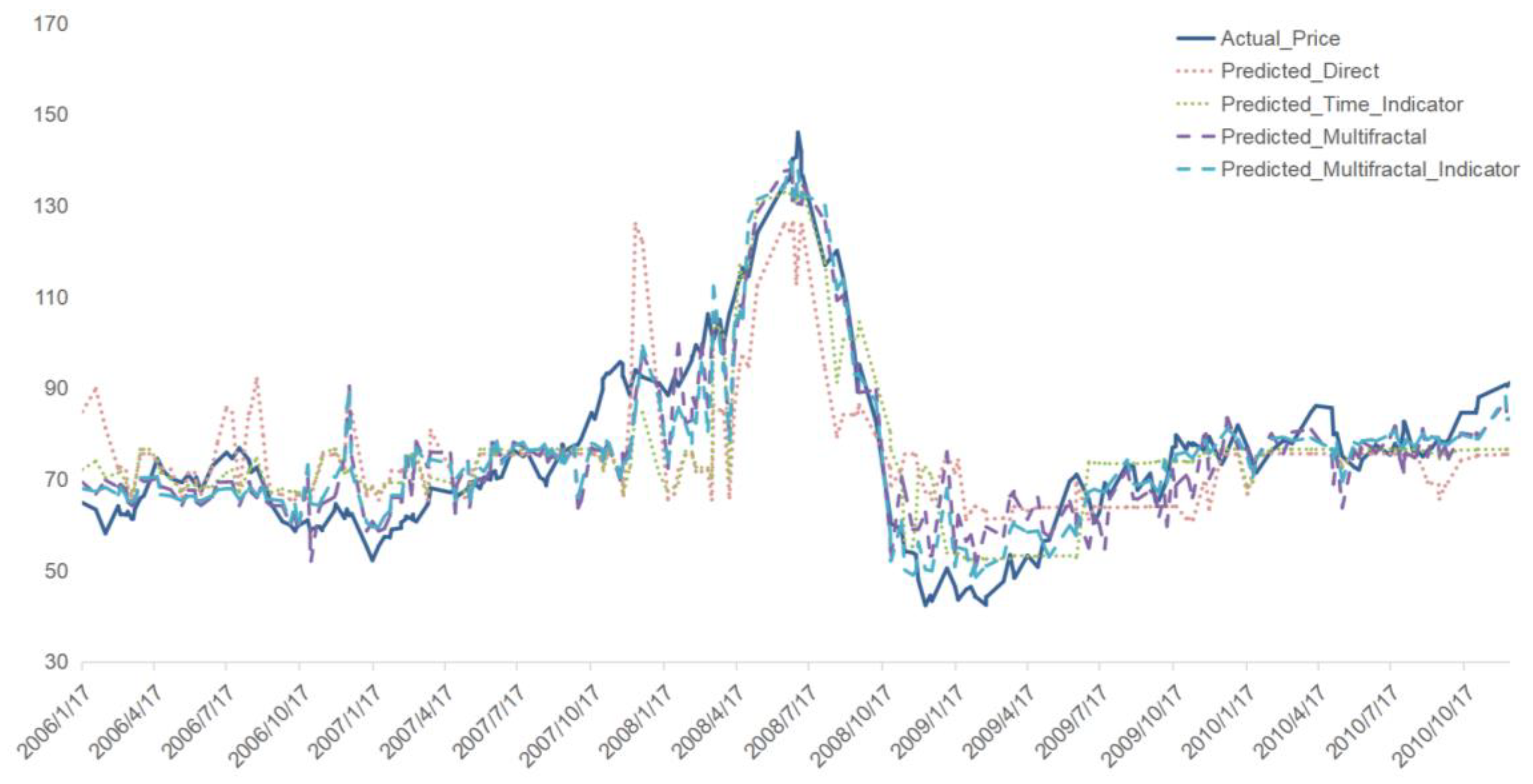
Figure 9.
Predictive Results for Brent Oil Prices during Period II.
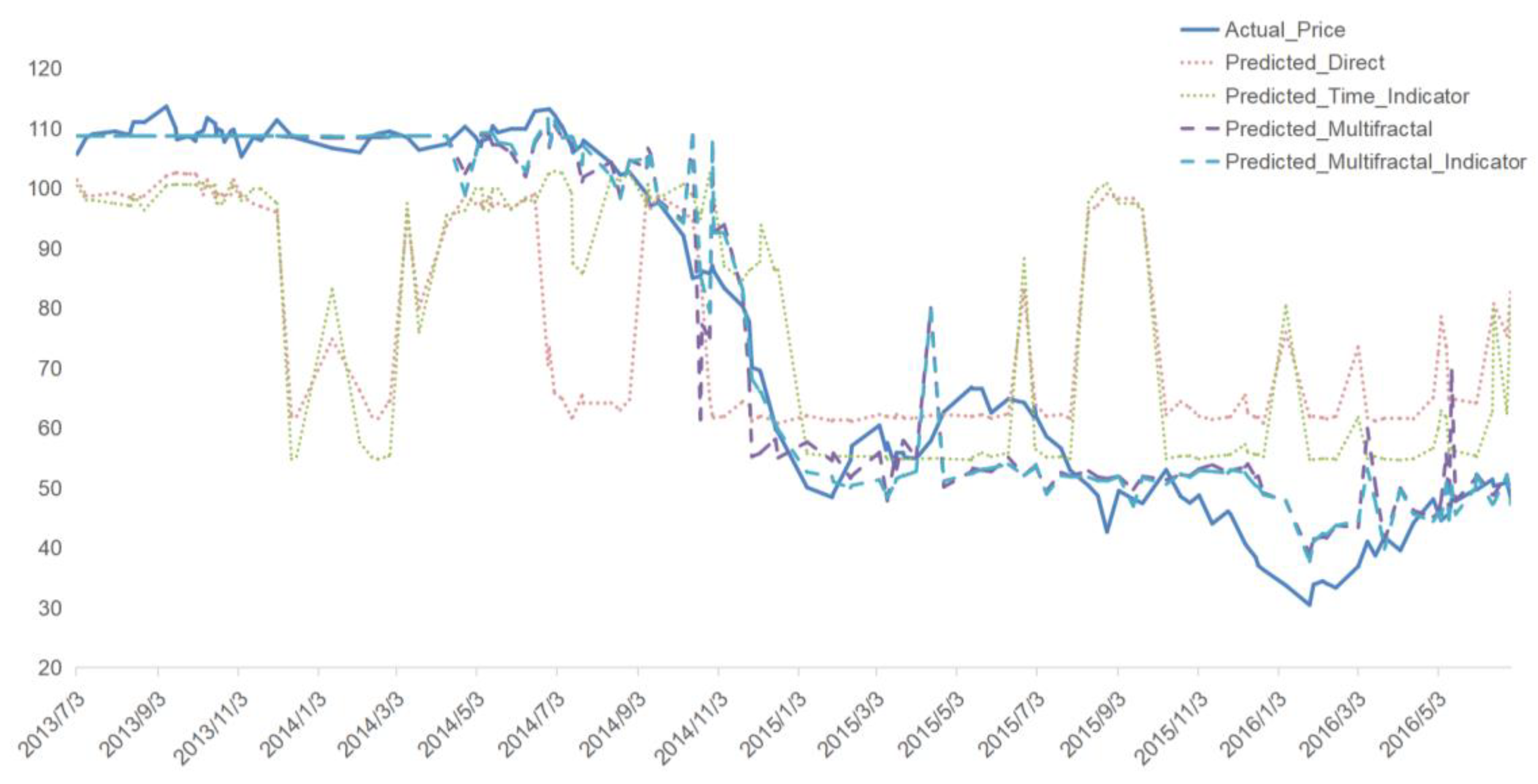
Figure 10.
Predictive Results for Brent Oil Prices during Period IV.
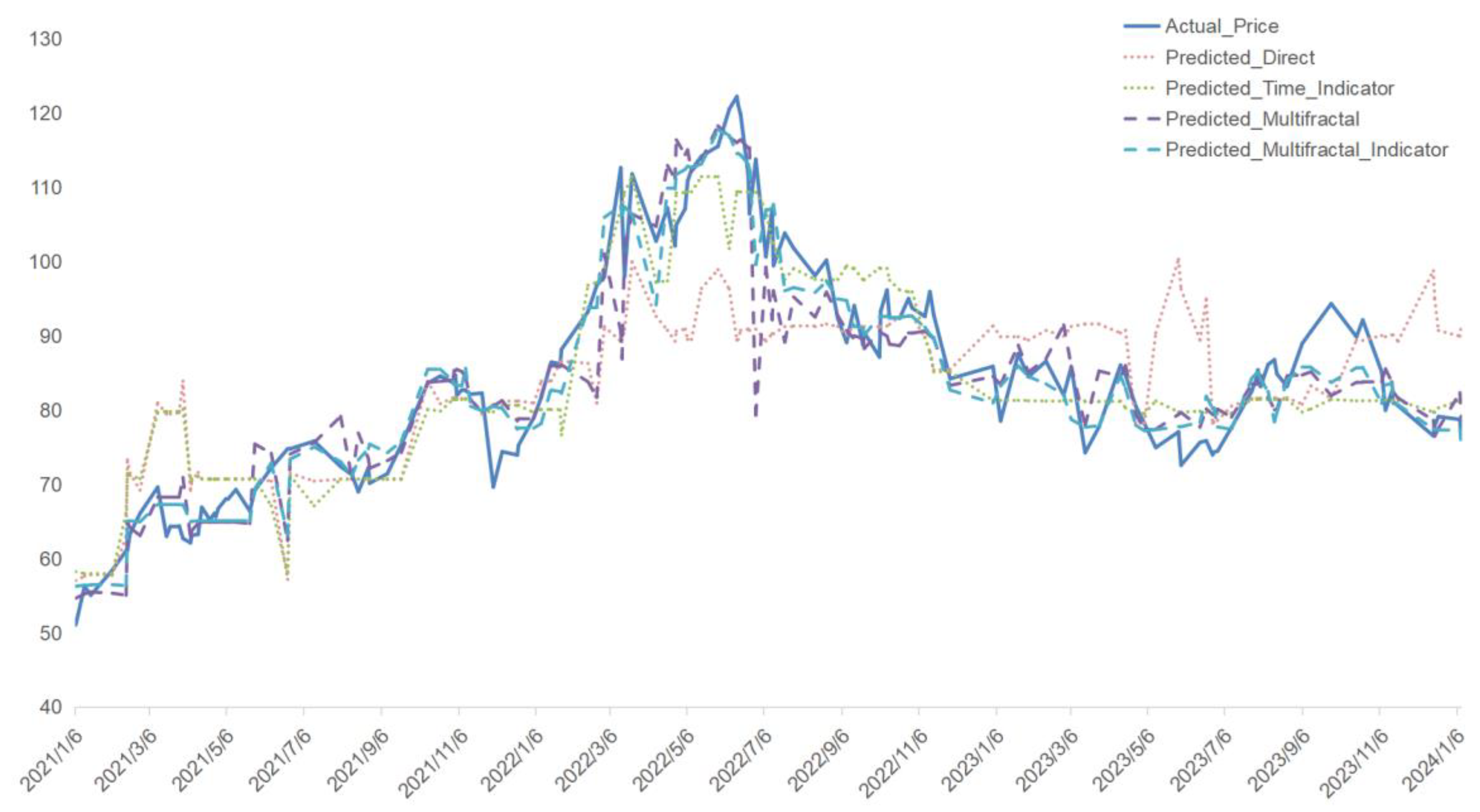
Figure 11.
MSE values for training and test sets across Period I-IV.
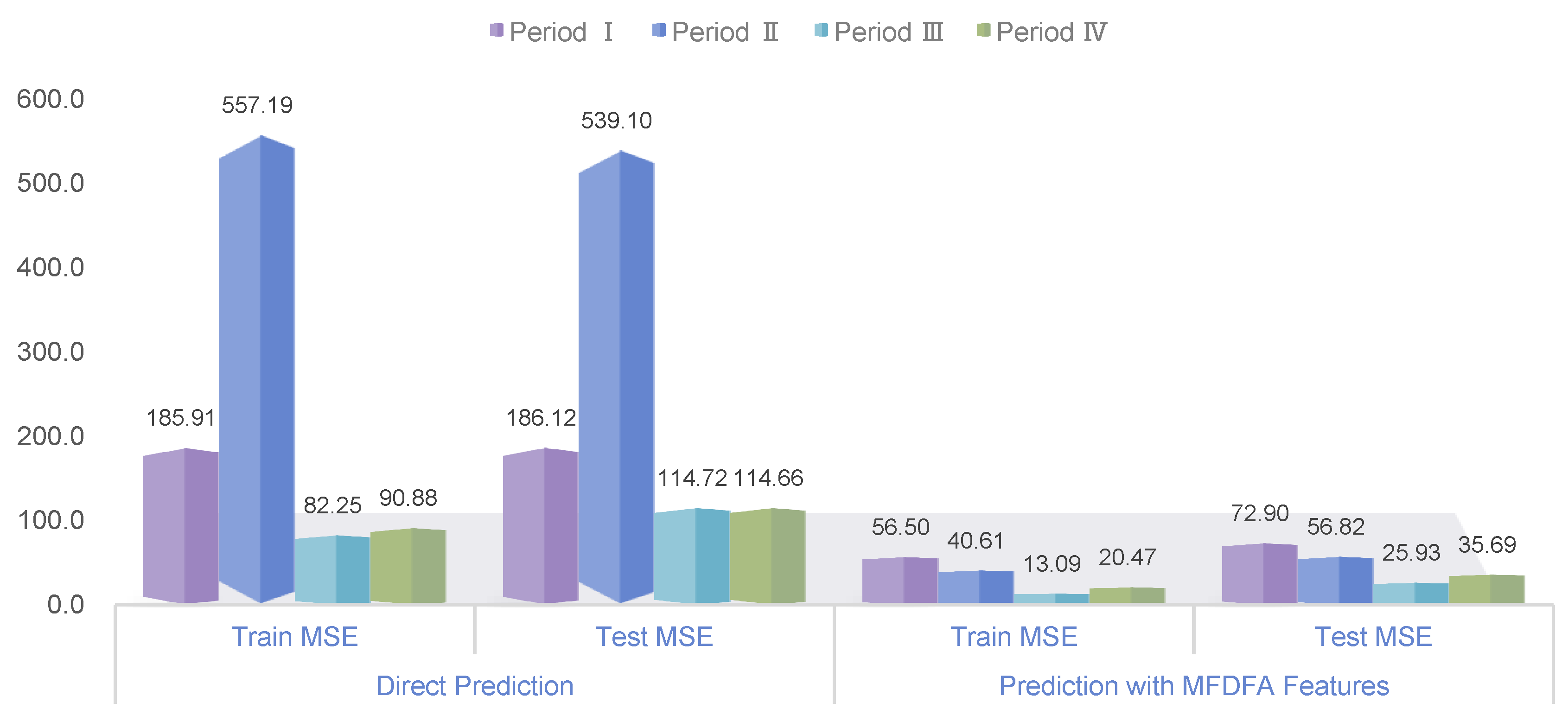
Figure 12.
R² scores for training and test sets across Period I-IV.
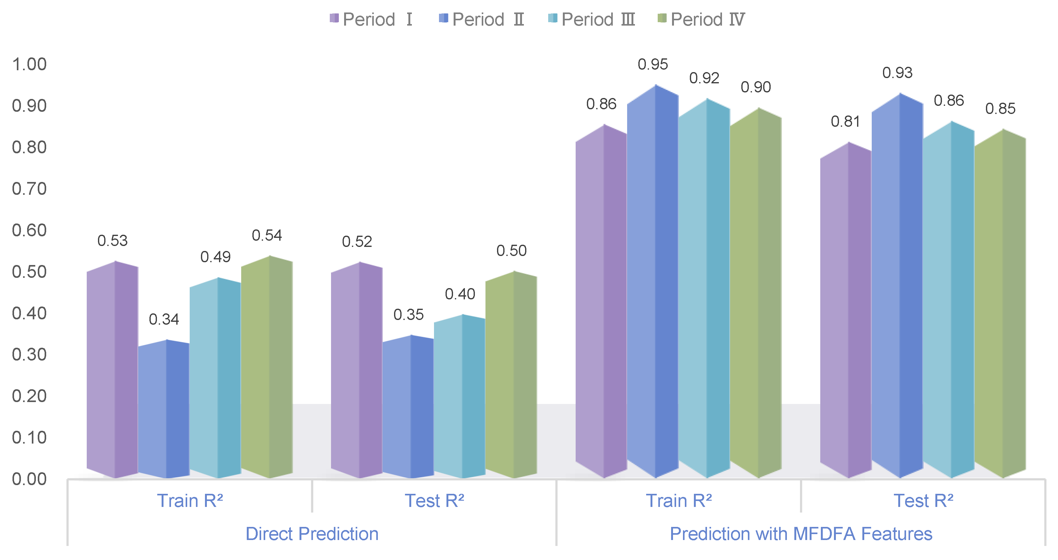
Figure 13.
Improvements in Mean Squared Error (MSE) and R² for Training and Testing Sets Across Four Periods After Incorporating Multifractal Features.
Figure 13.
Improvements in Mean Squared Error (MSE) and R² for Training and Testing Sets Across Four Periods After Incorporating Multifractal Features.
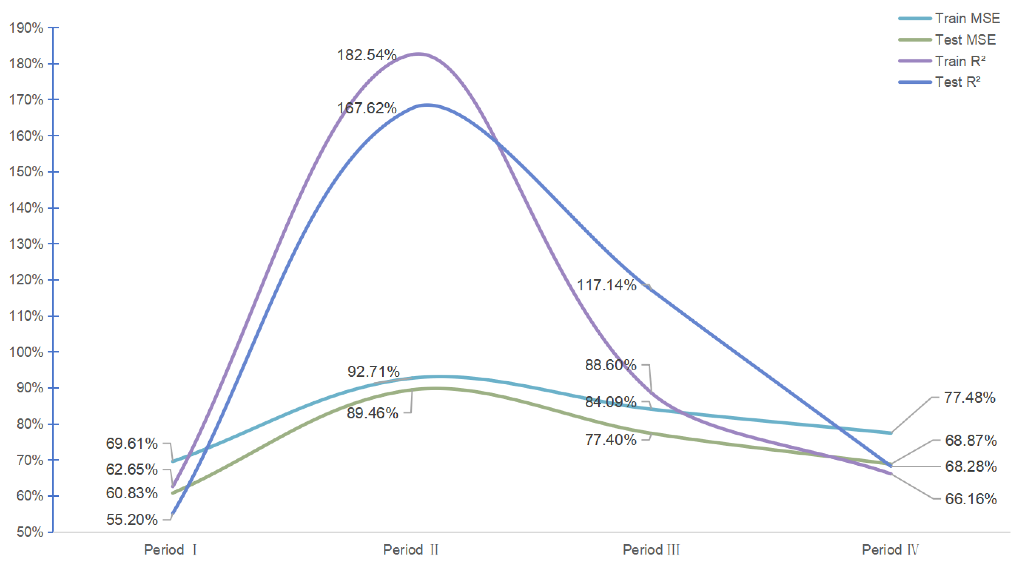

Table 1.
Distinct Historical Phases and Global Market Shifts.
| Period | Date Range | Global Event |
|---|---|---|
| Period I | 2006-01-01 - 2010-12-31 | 2008 Global Financial Crisis, which severely impacted financial markets worldwide. |
| Period II | 2013-06-30 - 2016-06-30 | 2014 Shale Oil Revolution, which altered the global energy supply. |
| Period III | 2019-01-01 - 2021-01-01 | COVID-19 pandemic, which led to unprecedented disruptions in global supply chains. |
| Period IV | 2021-01-01 - 2024-01-12 | 2022 Russia-Ukraine conflict, which introduced geopolitical uncertainty and significant energy price fluctuations. |
The table summarizes the four distinct periods analyzed, each characterized by major global events that significantly influenced financial markets. This table is used to provide context for understanding the complexities involved in the predictive modeling of Brent oil prices during these turbulent times.
Table 2.
Statistics of Tanker Freight Rate Returns.
| Series\Statistics | size | mean | Std. | Min. | Max. |
|---|---|---|---|---|---|
| BCTI | 6413 | 2.28e-05 | 0.02 | -0.57 | 0.29 |
| BCTI TC2 | 5014 | -2.37e-04 | 0.04 | -0.37 | 0.58 |
| BDTI | 6358 | 6.44e-05 | 0.02 | -0.38 | 0.24 |
| BDTI TD7 | 6234 | 8.27e-05 | 0.05 | -0.50 | 0.46 |
Table 3.
MF-DMA results for tanker freight rates.
| Title 1 | |||||
|---|---|---|---|---|---|
| BCTI | 0.90 | 0.48 | 0.61 | 0.29 | 0.77 |
| BCTI TC2 | 0.86 | 0.23 | 0.39 | 0.47 | 0.70 |
| BDTI | 0.58 | 0.28 | 0.52 | 0.06 | 0.34 |
| BDTI TD7 | 1.03 | 0.28 | 0.50 | 0.53 | 0.81 |
| BDTI 1998-2010 | 0.60 | 0.29 | 0.54 | 0.06 | 0.35 |
| BDTI 2010-2023 | 0.72 | 0.35 | 0.62 | 0.10 | 0.45 |
Disclaimer/Publisher’s Note: The statements, opinions and data contained in all publications are solely those of the individual author(s) and contributor(s) and not of MDPI and/or the editor(s). MDPI and/or the editor(s) disclaim responsibility for any injury to people or property resulting from any ideas, methods, instructions or products referred to in the content. |
© 2025 by the authors. Licensee MDPI, Basel, Switzerland. This article is an open access article distributed under the terms and conditions of the Creative Commons Attribution (CC BY) license (http://creativecommons.org/licenses/by/4.0/).
Copyright: This open access article is published under a Creative Commons CC BY 4.0 license, which permit the free download, distribution, and reuse, provided that the author and preprint are cited in any reuse.


