
Submitted:
12 February 2025
Posted:
12 February 2025
You are already at the latest version
Abstract
High pressure and temperature (PT) experimental charges are valuable systems made of minerals, often with quenched melt, and/or a fluid. They are synthesized to inform petrological solid-state, melt-forming and/or fluid-assisted processes occurring deep within the Earth. Here we explored the utility of phase mapping for analysis of high PT charges. We compared phase maps obtained with automated mineralogy software of scanning-electron-microscopes and developed an open-source software workflow. This generates phase maps from combined back-scattered-electron and 4-element maps. Phase maps were constructed for a sub-solidus assemblage, a charge containing a small percentage of melt, and a melting experiment that failed to reach thermal equilibrium. For the sub-solidus experiment, the phase map returned an accurate modal mineralogy. For the quenched melt experiments, the phase map located low abundance phases and identified best-suited targets for chemical analysis. Using modal mineralogy of sub-regions on maps and mutual neighboring relationships, the phase maps helped to establish equilibrium conditions and verify melting reactions inferred from mass balance. We propose phase maps as a valuable additional documentation tool for publishing high PT experiments, as they can help identify rare phases and discover reactions. We conclude with a set of recommended instrument settings for high-quality phase maps on small experimental charges.
Keywords:
experimental petrology
; phase mapping
; scanning electron microscope
; back-scattered-electron
; modal mineralogy
; melting reactions
; thermal gradient
; mass balance
; instrument
1. Introduction
High pressure and temperature (PT) experiments on chemical compositions relevant to key magmatic processes underpin the quantitative understanding of generation of melts and igneous differentiation [1,2,3,4,5]. They also contribute very important information about the role of critical fluids in the formation of rocks that are unusually enriched in incompatible elements, including mineralization [6,7,8,9,10]. At solid-state conditions, high PT experiments are the foundations for quantitative thermobarometry [11,12,13], allowing metamorphic petrologists to deduce PT conditions experienced by rocks that have been exhumed from the roots of mountain belts. High PT experiments also inform the partitioning of trace elements between phases and thereby provide the fundamental knowledge for geochemical modelling.
To a first order, high PT experiments conducted in large piston cylinders and multi-anvil devices become more technically challenging with increasing P and/or T conditions for a variety of reasons. At Ps above ca. 4 GPa and Ts substantially above the melting point of the system of the experimental charge, it is common for experiments to be unsuccessful due to malfunctioning of the equipment, lack of equilibration in the charge, excessive thermal gradient, or leakage or failure of the assembly containing the charge. Due to this technical difficulty, experimental gaps remain in our knowledge of melt generation processes. Successful experiments are therefore valuable, representing substantial investment of resources and time.
The key results obtained from high PT melting experiments are the modal abundances of the generated phases (solids, liquid, and where applicable fluid(s)), their compositions (in major and trace elements) and the stoichiometry of reactions that generated the liquid. In preparation for analysis, the recovered assembly is cast into a resin disc that is then ground to expose the charge and finely polished for electron-beam and further analysis. Experimental charges therefore cannot typically be investigated with transmitted light microscopy and are instead studied with electron-beam techniques, most notably scanning electron microscopes (SEM) and electron microprobe analyzers (EMPA). The use of electron beam analysis also addresses the generally small grain size (<50 microns) of phases constituting experimental charges.
The routine analytical approach is to first inspect the charge with SEM back-scattered-electron (BSE) detector images, with which phases of different composition (mean atomic number) are visualized in different grey scale levels. This allows the experimentalist to decide whether the experiment was likely successful and to identify representative targets for chemical analysis by EMPA. Once all measurable phases have been quantitatively analyzed and equilibrium has been established, the modal abundance can be calculated from the knowledge of the system starting composition and the compositions of the individual phases. This mass balance approach [14] is well tested and proven [15] but does carry some limitations for phases in low modal abundance (e.g., low degree partial melts) and for major elements (e.g., Ti) present at low concentrations and in cases where elements were lost to the capsule (e.g., Fe).
One further limitation of inspecting the charge with SEM BSE is that the resulting images are greyscale, making it difficult for the human eye to distinguish between subtly different shades of grey, potentially representing different phases that may have a very similar mean atomic number. In automated mineralogy applied to natural rocks or grain mounts, it has become routine to visualize the phase assemblage and mutual geometric grain contact relationships (liberation) with phase maps generated by combining SEM-BSE with SEM energy-dispersive-spectroscopy (EDS). This approach takes advantage of the SEM-BSE to define grains and their boundaries, and the SEM-EDS to distinguish phases of very similar BSE response and accessory phases of very different chemistry with the EDS spectra [16]. In modern SEMs configured for automated mineralogy, dedicated software provides a convenient workflow of acquisition of data, generation of elemental maps, and user-assisted production of phase maps, including for entire thin sections [17].
The aim of this study was to test the ability of SEM-based automated mineralogy to generate phase maps for experimental charges produced at 5 GPa on a moderately refractory model mantle composition, dominated by two oxides: MgO (38.2 wt%) and SiO2 (45.5 wt%) containing two silicate minerals (olivine and orthopyroxene) of near-identical mean atomic number. We evaluated the results of two commercial software solutions, tested SEM-BSE and SEM-EDS analytical settings and optimized an open-source software approach (image analysis pipeline) developed for measuring phase relationships in rock thin sections to the fine-grained experimental charges. Finally, we compared the resulting modal abundance estimates with the conventional mass balance approach and explored the utility of phase maps to extract value from an ‘unsuccessful’ high PT experiment.
2. Materials and Methods
Three experimental charges were investigated for this study. They were selected from a much larger isobaric 5 GPa suite of mantle peridotite melting experiments, which will be reported elsewhere alongside the experimental details. The experiments were conducted in a modified high-pressure, 500-tonne end-loaded piston cylinder at the Australian National University (ANU). Further information on the piston cylinder apparatus and assembly materials used in this study were reported elsewhere [13,18].
For this technical study, we selected one successful representative experiment each from above (UHP40) and below (UHP32) the solidus and included an additional ‘failed’ melting experiment (UHP21) that did not pass the thermal equilibrium test. In all cases, due to the simple ultramafic system composition (GKR-001, Table 1), only very few phases were expected: olivine, orthopyroxene, garnet, clinopyroxene, melt and possibly Cr-rich spinel. Observed phase relations were compared to those thermodynamically modelled with MAGEMin [19] based on the igneous dataset [20]. For EMPA analysis and imaging with SEM-BSE, the charges were prepared as follows: after the run, the recovered sample was mounted into epoxy and polished in water using 800- and 1000-grit sandpaper to expose the charge. After exposing a small section of the charge, polishing continued with 1200- and 2500-grit sandpaper to avoid sample loss and excessive mineral plucking during polishing. The final polishing stage was done with diamond pastes (6, 3, 1, and 0.25 μm). Before carbon-coating the samples, the quality of the polish was carefully assessed using a reflected light microscope.
The composition of the main phases (olivine, pyroxenes and garnet) was analyzed with standard EMPA protocol at the ANU and is listed in Table 1. For this study, the sole purpose of the chemical compositions was to calculate modal abundance via mass balance (Table 1). Petrological implications will be discussed with the full suite of experiments.
After EMPA analyses, the samples were investigated by SEM-BSE and -EDS at QUT’s CARF laboratory on a Tescan TIMA Field-Emission-Gun (FEG) SEM [17], equipped with three EDS detectors. After experimentation, the preferred setting for this project’s routine phase mapping imagery was as follows. For BSE (with Image Snapper), the acceleration voltage was 15 kV, at a beam intensity of 12.0, and with BSE scan setting S7 (100 μs/pixel). For EDS mapping, the acceleration voltage was 25 kV at a beam intensity of 19.9, and an X-ray count to 4,000. For the small experimental charges (typically ca. 1.2 x ca. 0.6 mm), the BSE acquisition took 40-90 minutes and the EDS maps 30-80 minutes. A series of exploratory scans were conducted to evaluate the influence of BSE scan speeds, EDS acquisition modes and EDS count rates on resulting phase map quality. One sample was additionally analyzed on a Hitachi SU7000 field emission SEM equipped with the Bruker AMICS automated mineralogy system at UQ Natural Resources Innovation Characterisation Hub (NRICH), again, exploring different combinations of BSE scan speeds and EDS acquisition modes for optimal phase maps on experimental charges.
In addition to the phase maps produced with the proprietary software of the SEMs, we devised an open-source software method for user-informed pixel classification that was optimized for fine-grained samples. The approach involved the following steps.
We began by acquiring scan setting S7 (100 μs/pixel) BSE images (25% overlap between frames) using the Image Snapper add-on in the MIRA3 software. The resulting tiles were stitched with the ImageJ2 software TrakEM2 plugin using globally optimized intensity-based registration [21] to achieve a high-quality alignment. Next, we acquired a separate TIMA experiment using the dot-mapping EDS approach (accelerating voltage 25 kV, pixel spacing 0.5 μm, dot spacing 1.5 μm and field width 100 μm) and generated individual elemental X-ray intensity maps. Considering the chemistry of the phases, four element X-ray K-line maps were found sufficient for phase recognition (Al for garnet, Ca for clinopyroxene, and Mg and Si to distinguish between olivine and orthopyroxene). These were auto-stitched in the TIMA project, manually selected within the interface, and sequentially exported at the original resolution without ancillary information (legend, scalebar, etc.).
The high-quality BSE montages were then used as fixed images for registration of the element X-ray K-line maps using control-point manual registration following a non-rigid transformation in BigWarp [22], a plugin extension of ImageJ2 [23]. The now co-registered montages (one BSE and 4 element X-ray layers) were imported into QuPath software [24] projects and stacked as multi-channel images. The ‘Interactive image combiner Warpy’ extension [25] was deployed to generate a virtual ‘overlay’ (not saved in the permanent memory). Next, each phase category present was annotated (12-15 polygons each) with the brush and wand tools. For this, the interactive combined viewer was used to identify the phase on the BSE image with reference to the multi-element X-ray intensity maps. Care was taken to annotate each defined grain on the BSE image exactly to the well-defined grain contour, avoiding annotating grain boundaries. Finally, the pixel classifier tool was deployed at ‘very high’ resolution (1 segmented pixel = 2 x 2 original pixels) using a random trees model. The resulting semantic segmentation maps were transferred to MatLab to obtain the phase maps, modal mineralogy [26], multiresolution association matrices [27], and adjacency (or accessibility) maps [28]. All QuPath projects, intermediate files, and maps are provided in the data repository (https://zenodo.org/records/14822997).
3. Results
3.1. Evaluating BSE Scan Speeds and EDS Acquisition Settings
For commercial high-throughput or large area applications of automated mineralogy, the SEM acquires a grid of adjacent frames with user-defined overlap. For each frame, the SEM first acquires a BSE image which is then pre-segmented into areas of similar greyscale (‘segments’). Algorithms then find representative points within these polygons for EDS acquisition – typically called EDS ‘dot’ maps. After acquisition of all the frames, their nominal stage x-y positions are used to construct the mosaic. Different options exist to merge grains of equal compositions along adjacent frames into phases. This is a significantly more economical approach for covering large area phase maps than a brute force high-spatial resolution grid EDS analysis (variably called ‘high resolution’ or ‘grid’ mapping, among others) but it relies on stable probe current delivered by the FEG [17]. Regardless, irrespective of the FEG-SEM instrument and proprietary phase mapping software used in this study (Tescan/TIMA and Hitachi/ Bruker AMICS), we found stitching errors in the BSE montages of at least some of the experimental charges. Mostly, they were small x-y offsets but in some cases, led to a repetition of features in the phase maps. The stitching errors reflect the rapid way in which the proprietary software generates BSE montages from nominal frame positions without intensity- and feature-based registration and without operator input. For academic research on high value targets, however, the time effort involved in producing the best possible BSE montages is trivial.
For this reason, we obtained grids of unstitched BSE frames on the Tescan TIMA MIRA3 instrument with wide (25%) areal overlap, that were individually read, accurately montaged, and registered. To find the fastest BSE scanning rate on this SEM still yielding acceptable results for phase mapping of our charges, we performed a series of tests on a small area of the finest-grained, sub-solidus charge UHP32. These experiments encompass unreasonably fast to excessively slow scanning rates and results are shown on Figure 1.
Qualitative visual inspection suggests that scan speed settings S3 to S5 are too fast, producing noisy BSE images with poorly resolved grain boundaries. At the slow scan speed end, settings S9 and S10 offer limited return on time investment over S8. For example, area scans performed in S9 take 2.9 times longer than in S8 and S10 scans take 9.1 times longer than in S8. Realistic scan speed rates were therefore judged to be S6 to S8. To more thoroughly evaluate the effects of scan speed setting on grain boundary identification and grey scale level differentiation, we extracted grey-scale intensity line profiles across sample UHP32. Figure 2 compares those obtained with BSE scan speed settings S6 through to S10.
The comparison shows that noise in scan speed setting S6 still obscures phase boundary definition but that scan speed settings S7 and S8 accurately locate phase boundaries. These two settings were therefore investigated further. Of note is that even with the slowest scan speed settings S9 and S10 (lowermost profiles in Figure 2), the overall BSE intensity of orthopyroxene is not distinguishable from that of olivine. This peculiarity of the charges studied here contributed to the dearth of BSE contrast. For quantitative evaluation of the most time effective accurate acquisition settings, individual phase maps were constructed with a permutation of BSE and EDS settings. A subset of the resulting phase maps is shown on Figure 3.
Two separate ground truth phase maps were generated. The first used a routine Tescan TIMA setting which combines fast BSE scanning (S4) with slow, high-spatial resolution EDS mapping (pixel spacing 0.5 μm). Despite substantial effort with selecting different combinations of element maps and phase map settings, it proved difficult to; (i) avoid generating artificial phases along grain boundaries (mixed pixels = ‘mixels’), (ii) define less jagged (binary) grain boundaries, and (iii) avoid excessive attribution of pixels to ‘holes’. The default spectral library search incorrectly attributed all olivine and orthopyroxene pixels to the ‘olivine’ class, while clinopyroxene pixels were split into ‘diopside’ and less abundant ‘actinolite’. Therefore, a custom library was built for the phases shown in Figure 3, which required testing and adding compositional rules and the ‘clinopyroxene mixels’ class. The second ground truth map was generated with the open-source software workflow combining the best BSE image with the high-resolution EDS elemental maps (a combination of Ca, Al, Si and Mg). This resulted in a crisp phase map, with realistic appearing grain boundaries, few holes and a lack of ‘mixels’. It also managed to discern many olivine-olivine grain boundaries due to their fine surface irregularities being classified as holes. Additional phase maps were then generated with the open-source software workflow for a permutation of BSE scan setting imagery (S7 to S9) and high-resolution and dot-mapping EDS element maps. Figures 3c and 3d compare the BSE S7 scan setting maps combined with the two EDS element maps. The visual comparison shows that they are indistinguishable to the human eye. They both show crisp grain boundaries (derived from the common BSE image). Finally, despite the much lower spatial resolution of the dot-based elemental maps, the resulting phase map (Figure 3d) appears indistinguishable from that obtained with the higher-quality high-resolution EDS map (Figure 3c).
For the final evaluation of preferred acquisition settings, the modal abundances (wt%) of the four rock forming minerals were calculated from pixel numbers on the phase maps and theoretical densities (olivine = 3.310; orthopyroxene = 3.338; clinopyroxene = 3.175; garnet = 3.600) for statistical comparison (Figure 4). Binary plots of BSE S7 and S8 with high-resolution EDS mapping modal abundances are compared to the BSE S10 with high-resolution EDS mapping ground truth modal abundance. This showed very good proportionality with both comparisons (Figure 4a) on the small representative area on sample UHP32 (Figure 3) with no statistical difference between the S8 and S7 BSE scan speeds. Binary plots of BSE S7 with high-resolution and dot EDS mapping were next compared to BSE S10 with high-resolution EDS. Again, this showed no statistical difference in the quality of the regression.
3.2. Phase Maps and Modal Mineralogy for Successful Experiments
The full phase map for sub-solidus sample UHP32 (Figure 5) made with the open-source software demonstrates a granular texture and a mode dominated by olivine and clinopyroxene. The frequency of pixels was used to determine the modes of the arbitrarily defined upper ‘Zone A’ and lower ‘Zone B’, the former with higher orthopyroxene abundance. The modes of both zones are displayed on the left-hand side in panels (a) and (b) of Figure 5. The comparison demonstrates that modally more abundant orthopyroxene in ‘Zone A’ is largely present at the expense of the compositionally similar clinopyroxene (Table 1). We note that the presence of orthopyroxene could be overlooked when inspecting ‘Zone B’ under real-time BSE on an EMPA, recalling that it has an indistinguishable BSE greyscale from olivine (Figure 2).
In the successful melt-present experiment UHP40, the open-source software generated phase map (Figure 6) again reveals some phase differentiation, with the upper layer (‘Zone A’) richer in orthopyroxene and melt and poorer in clinopyroxene and the lower, melt-poor layer (‘Zone B’) much more similar in mode to the subsolidus sample (Figure 5). Like in sample UHP32, the presence of orthopyroxene is largely at the expense of clinopyroxene and, to a lesser extent, garnet. The association matrices show that all phases are in contact with each other, but with a clearly defined preferred association of melt, garnet and clinopyroxene, which will be elaborated later.
3.3. Phase Map for Experiment Which Did Not Experience Thermal Equilibrium
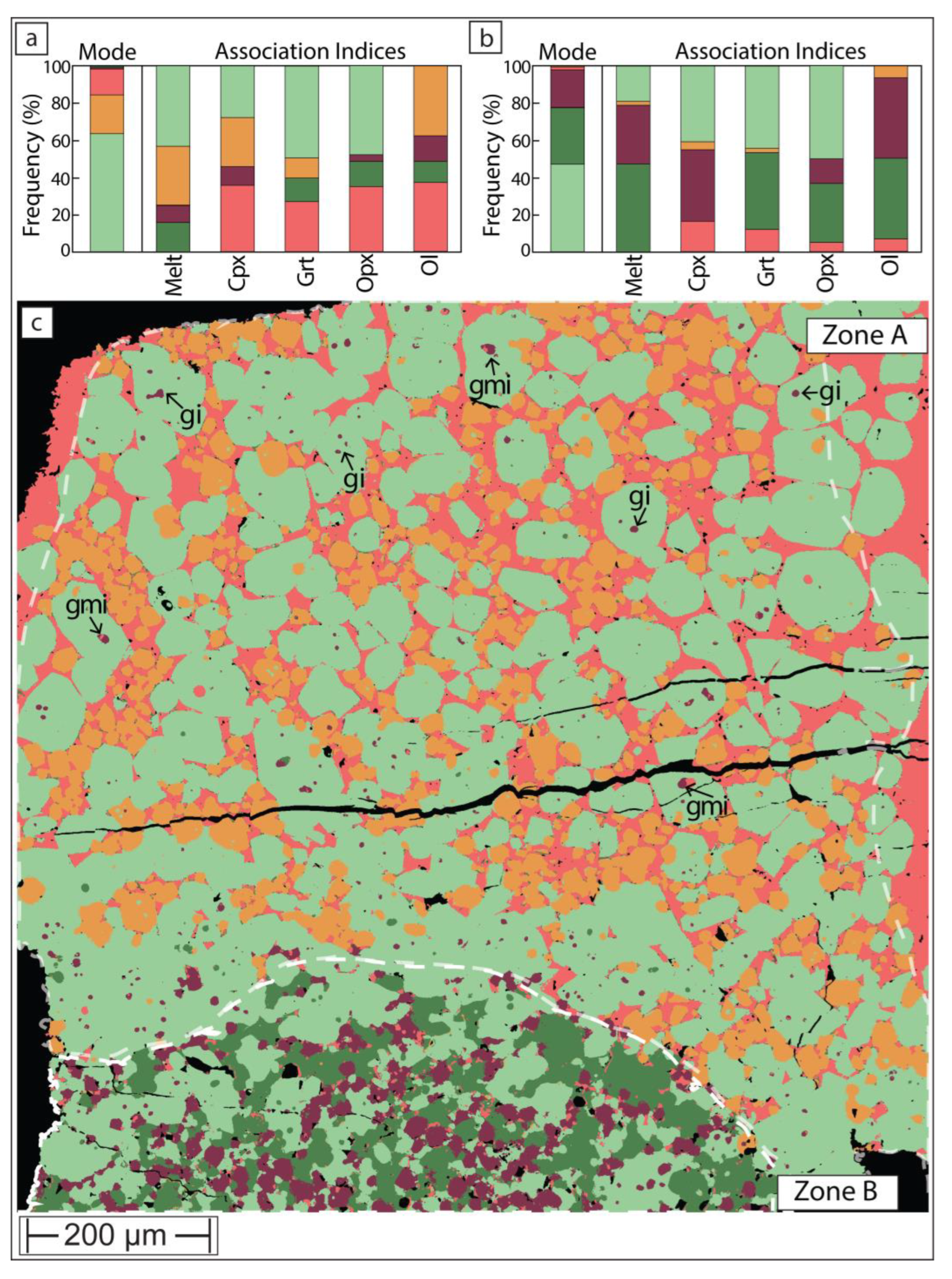
Sample UHP21 experienced heterogenous thermal conditions across the charge. In this instance, the bottom of the charge reached a lower temperature than the top. In experiments above the solidus, such as here, this is typically visualized in BSE with a strong contrast in melt distribution and a pronounced preferred spatial distribution of phases. In the case of UHP21, the bottom of the charge is both brighter and darker in BSE due to the high abundance of garnet (bright) and clinopyroxene (dark), while the bulk of the charge is composed of olivine, orthopyroxene and melt that formed at more elevated temperature.
On the phase map produced with the open-source software method (Figure 7), the charge can be separated into two zones. The cooler temperature ‘Zone B’ is composed predominantly of olivine, clinopyroxene and garnet with very little melt (2.3 wt%) and even less orthopyroxene. By contrast, the upper ‘Zone A’, which occupies the bulk of the charge, is mostly composed of olivine, orthopyroxene and melt (14 wt%). In the interpreted higher temperature ‘Zone A’, rare garnet (1 wt%) only exists as small inclusions in much larger olivine grains and clinopyroxene (0.9 wt%) is largely confined to inclusions within olivine in proximity to ‘Zone B’. Some clinopyroxene also exists along orthopyroxene-melt grain boundaries, where it likely formed as a quench product from the melt.
The distribution of these phases suggests that the charge formed over a temperature window that covers a major melt forming reaction. This predominantly consumed clinopyroxene and garnet and produced peritectic orthopyroxene. The stoichiometry of this reaction at 5 GPa in lherzolite composition KR4003 was thermodynamically modelled [29] as follows:
0.31 olivine + 1.7 clinopyroxene + 0.19 garnet = 1 melt + 1.2 orthopyroxene,
This appears in good qualitative agreement with the distribution of phases in the map of sample UHP21 and illustrates that ‘failed’ experiments exposing thermal gradients may contain value in terms of verifying reactions that are normally calculated based on mass balance [30] rather than microstructural observations.
Figure 7.
Phase maps of sample UHP21, for color key see Figure 6. For statistical purposes (modal abundance and phase association), the map was subdivided into ‘Zone B’, representing lower temperature and a melt- and orthopyroxene-rich ‘Zone B’. Garnet and garnet-melt inclusions in olivine are annotated with ‘gi’ and ‘gmi’, respectively.
4. Discussion
The discussion is structured into two sections, the first delving deeper into the utility of phase maps to investigate high PT experimental charges and the second focusing on instrument settings for generating phase maps suitable for experimental charges.
4.1. Insights from Phase Maps of High PT Charges
Beginning with the subsolidus sample UHP32, the modal abundance estimated from its phase map (Figure 5) compares very well with that obtained from mass balance (Table 1). The two estimates correspond closely (Figure 4c) and yield a regression slope of 0.9972 with an r2 of 0.9987. This demonstrates that although the phase map is obtained from a 2-dimensional slice through the charge, it is a valid representation of the overall system and of the phase chemistries, which inform the modal mineralogy obtained via mass balance. More importantly, the very good agreement between the methods is a strong test of the accuracy of the starting composition. The production of synthetic rock system compositions can involve many steps that include multiple weighing and handling of powders with associated uncertainties. The tight agreement between the two independent methods of estimating modal mineralogy confirms the accuracy of the starting composition and the EMPA phase chemistry. Furthermore, the agreement in modal mineralogy also confirms the isochemical nature of the experiment, at least for the major rock forming oxides. Namely, it is not uncommon for high T experimental charges to lose redox-sensitive species (e.g., Fe) to the assembly, resulting in undesired unintentional change in the system chemistry, see e.g., [31]. Independent modal abundance estimate agreement warrants against loss or gain of major system components.
A final strength of phase maps is that they can be used to quantify mineral associations. This is an active research field in mineral processing, liberation and exploration [32] whereas in metamorphic and igneous petrology, mineral association matrices have traditionally been used to test local equilibrium e.g., [33]. The spatial information contained in computed phase maps can be used to calculate quantitative information about mutual mineral (or phase) contacts. For sub-solidus sample UHP32, the mineral association matrix (Figure 5) confirms that all four rock forming minerals are in mutual contact. In both the upper and lower ‘Zones A’ and ‘B’, pixels of the most abundant mineral olivine are in contact with all other minerals with no clear preferences. By contrast, ortho- and clinopyroxene are in preferential contact, sharing more pixel boundaries than could be expected from modal abundance. The surprisingly uneven distribution of ortho- and clinopyroxene across ‘Zone A’ and ‘B’ could have two mutually inclusive reasons. First, very minor heterogeneity in the starting mixture (e.g. Ca) could cause significant changes in pyroxene modes, considering the overall similarity in chemistry of both pyroxenes. Secondly, at the PT conditions of these experiments, ortho- and clinopyroxene have near-identical entropies and very similar enthalpies [34], meaning that the minimum energy of the system is insensitive to the ratio of the pyroxenes.
Turning next to sample UHP 40, we note that the agreement between mass balance and phase map-derived modal abundance is inferior (Table 1 and Figure 4c). The modal abundance estimates agree well for the two most abundant phases (olivine and clinopyroxene) but diverge for garnet, orthopyroxene and melt. This is most likely explained by the unrepresentativeness of the 2-dimensional exposure through the charge. According to mass balance, this experiment produced 7.7 wt% melt, yet the phase map only identified 3.4 wt%. This is almost certainly due to heterogeneous distribution of melt, which tends to coalesce towards the edges of charges, in this case underrepresented in the exposed surface of the charge. Instead, the phase map overestimates orthopyroxene and garnet. However, the effort to produce a phase map (ca. 3 hours SEM instrument time and ca. 3 hours work for segmentation) is still justified because of the clarity with which phases can be targeted for EMPA analysis. With respect to charge UHP40, the power of the phase map (Figure 6) is illustrated with two examples. First, within ‘Zone B’, melt is in very low abundance, but the phase map can guide the analyst to the largest ‘films’ or pools of it ahead of operating the EMPA. Second, the phase map illustrates that in ‘Zone B’, there are only very few grains of orthopyroxene (3.1 wt% modal abundance) while the BSE greyscale indistinguishable olivine is in much higher modal abundance (49.2 wt%). Such a low proportion of orthopyroxene would almost certainly have been missed based on BSE inspection alone. Thus, the availability of a phase map allows precise planning of EMPA spot selection, ensures all present phases are analyzed, and can save EMPA instrument time.
Finally, the phase map of UHP40 demonstrates gradation in mineralogy, principally, from a clinopyroxene-rich and very orthopyroxene-poor ‘Zone B’ at the bottom of the charge to an orthopyroxene-rich and clinopyroxene-poorer top left ‘Zone A’. This change in mineralogy is suggestive of melt-producing reaction (1), incongruently consuming clinopyroxene and generating peritectic orthopyroxene. This is supported by the phase association matrix. In both ‘Zones A’ and ‘B’ (Figure 6), clinopyroxene is dominantly in contact with melt, closely followed by garnet. The persistence of the melt + clinopyroxene + garnet spatial association thus suggests that melt migration was not excessive in this experiment. Namely, had melt mostly percolated towards the top of the charge away from the original site of melting, the preferential spatial association would not be expected.
Thermodynamic modelling of the GKR-001 system shows that at 5 GPa, 16.6 wt% melt forms over a temperature window of only 16°C. As can be seen from the corresponding modal abundance plot (Figure 8), over this melt generation interval, modelled clinopyroxene abundance in the solid drops from 32.2 wt% to 0 wt%, while orthopyroxene abundance increases from 0.5 wt% to 16.6 wt%. Modelling also predicts a more modest rate of garnet consumption compared to clinopyroxene, compatible with the phase distribution of ‘Zone A’ in Figure 6. Thus, although a small thermal gradient existed across the UHP40 charge, this was less than 16°C, as melt is already present at the bottom of ‘Zone B’ while some clinopyroxene persists on the top of ‘Zone A’. The rapid change in mineralogy and melt productivity over a very narrow temperature range seen in charge UHP40 illustrates the difficulty of experimentally determining the exact solidus of lherzolitic to mildly refractory peridotite at high P [35].
The final point of discussion concerns the ‘failed’ experiment UHP21. In this charge, the bottom ‘Zone B’ apparently resided close to the solidus (Figure 7), with similar modal abundances as in ‘Zone B’ of the successful experiment UHP40 (Figure 6). However, the bulk of the charge experienced substantially higher temperature with no clinopyroxene and hardly any garnet remaining. This suggests that in zone ‘A’, melting proceeded beyond the clinopyroxene-out reaction (Figure 8) that consumed all three remaining minerals. The stoichiometry of this type of reaction at 5 GPa in lherzolite composition KR4003 was thermodynamically modelled [29] as follows:
0.29 olivine + 0.47 orthopyroxene + 0.24 garnet = 1 melt
Because the clinopyroxene-consuming reaction (1) produces a lot of orthopyroxene (‘Zone A’ of Figure 6) in the GKR-001 system, reaction (2) apparently exhausted garnet before orthopyroxene was consumed. Therefore, as can be seen with annotations ‘gi’ on phase map of the ‘failed’ experiment (Figure 7), most garnets are preserved as non-touching inclusions within olivine. This suggests that the temperature in that part of the capsule did not reach that of the garnet-out reaction [29]:
0.30 garnet + 0.70 olivine = 1 melt
In other instances, garnet coexists with touching melt as olivine inclusions (labelled ‘gmi’ on Figure 7), suggesting the consumption of formerly touching pyroxene + garnet inclusions. Regardless of the intricacies of these inclusions and potential melting reactions, this example demonstrates that experiments that failed from the perspective of equilibrium because they formed over an undesirably wide temperature range, may still contain value. Their thermal disequilibrium creates microstructures that can help testing melting reactions hypothesized from mass balance.
4.2. Working Towards Optimized Operating Procedures for High-Quality Phase Maps of Experimental Charges
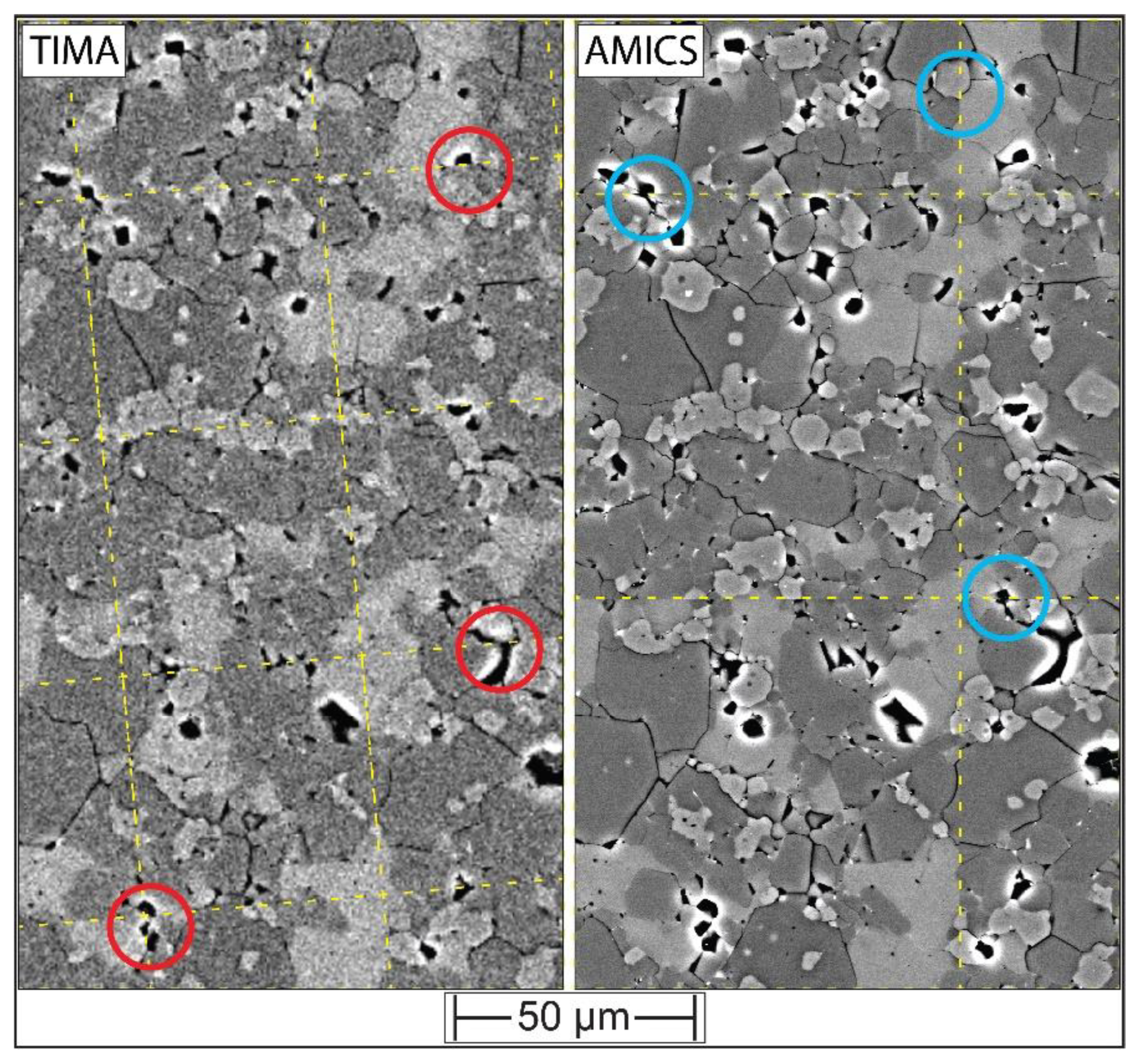
For a wider uptake of phase mapping of experimental charges, it is desirable for proprietary automated mineralogy solutions (e.g., Tescan TIMA, Bruker AMICS, Oxford Instruments AZtecMineral, Thermo Scientific Maps, etc.) to generate suitable phase maps without the need for external image analysis. This study obtained phase maps with two commercial systems, both of which returned accurate modal abundance estimates but also contained some artefacts, most commonly small x-y translation errors on the stitched mosaics. In Figure 9, such SEM-BSE montage registration offsets are illustrated for TIMA (red circles on a fast acquisition BSE) and AMICS (cyan circles on a slow acquisition BSE). They are caused by stage drift and can be compounded by lens distortion and poor beam alignment e.g., [36].
The frame offsets are minor and would not impact most automated mineralogy projects. However, misaligned mosaic inputs can negatively affect the ability of computer-assisted segmentation and classification into objects [37] because mineral grains that extend across poorly registered frames have unnatural straight boundary segments, right angles, or jagged contacts with neighboring grains. The misalignments in the simple x-y translation mosaics can be fixed offline with external post-analysis image processing e.g., [38]. However, this is only possible when the original overlapping frames are available (an example of a fixed AMICS montage is provided in the data repository). Regardless, when setting up a phase mapping project it is desirable to minimize stage travel and to find a good balance between the size of the filed of view versus spatial resolution and distortion. This may require some preliminary experimentation on a given SEM-EDS.
Figure 9.
Backscattered electron montages output from TIMA (left) and AMICS (right) software for the same area on sample UHP32. The dashed yellow lines trace the boundaries of adjacent frames. The circles in red (TIMA) and cyan (AMICS) show the locations of small ‘stitching’ errors.
Figure 9.
Backscattered electron montages output from TIMA (left) and AMICS (right) software for the same area on sample UHP32. The dashed yellow lines trace the boundaries of adjacent frames. The circles in red (TIMA) and cyan (AMICS) show the locations of small ‘stitching’ errors.
With both systems used in this study, the common observation was that the best phase maps were generated by combining relatively slow BSE scan rates with the ‘dot-mapping’ EDS approach. While it might, at first, seem counterintuitive to dedicate more time to the BSE acquisition, the consistent finding was that a high-quality BSE scan results in better initial segmentation and definition of fewer polygons that needed to be investigated for EDS analysis. For example, on the Bruker AMICS system, the phase map shown in Figure 10 was obtained in 11 minutes and 46 seconds combining 32 μs dwell BSE with dot EDS mapping. Using 16 and 8 μs BSE dwells with dot EDS mapping increased the acquisition times to 13 minutes and 7 seconds and 16 minutes and 27 seconds, respectively. This is because the faster BSE scans identified more watershed ‘segments’ (polygons) than necessary, thereby inflating the number of dot EDS analysis points. Furthermore, the faster dwell time BSE-based phase maps also showed more jagged and pixelated grain boundaries. On the Tescan TIMA, we found that 32 and 100 μs BSE dwell times resulted in quality BSE maps, while even longer dwell times offered no further advantage (Figure 2 and Figure 3). On AMICS, we also compared dot-mapping EDS with high-resolution or matrix mapping at very close pixel spacing (0.5 μm) and found no advantage, despite the substantially longer acquisition time (e.g., 122 minutes for a phase map the size shown in Figure 10). In summary, for the relatively small areas occupied by experimental charges, it is practical to obtain high-quality BSE imagery as the basis for rapid dot EDS mapping.
In terms of phase identification, we found that on both systems used, it is desirable to build up a bespoke mineral library rather than relying on reference to the system provided (large) mineral database. Because experimentalists generally have a good idea of the expected phases present in their charges, the comparison of EDS spectra with large reference databases is unnecessarily cumbersome. Furthermore, the reference libraries often contain multiple entries for solid-solution series (e.g., Mg- versus Fe-olivine) which can lead to unnecessary overcomplication when classifying pixels into phases. However, building a bespoke phase library does rely on the operator having a good understanding of EDS spectra and spectral interferences.
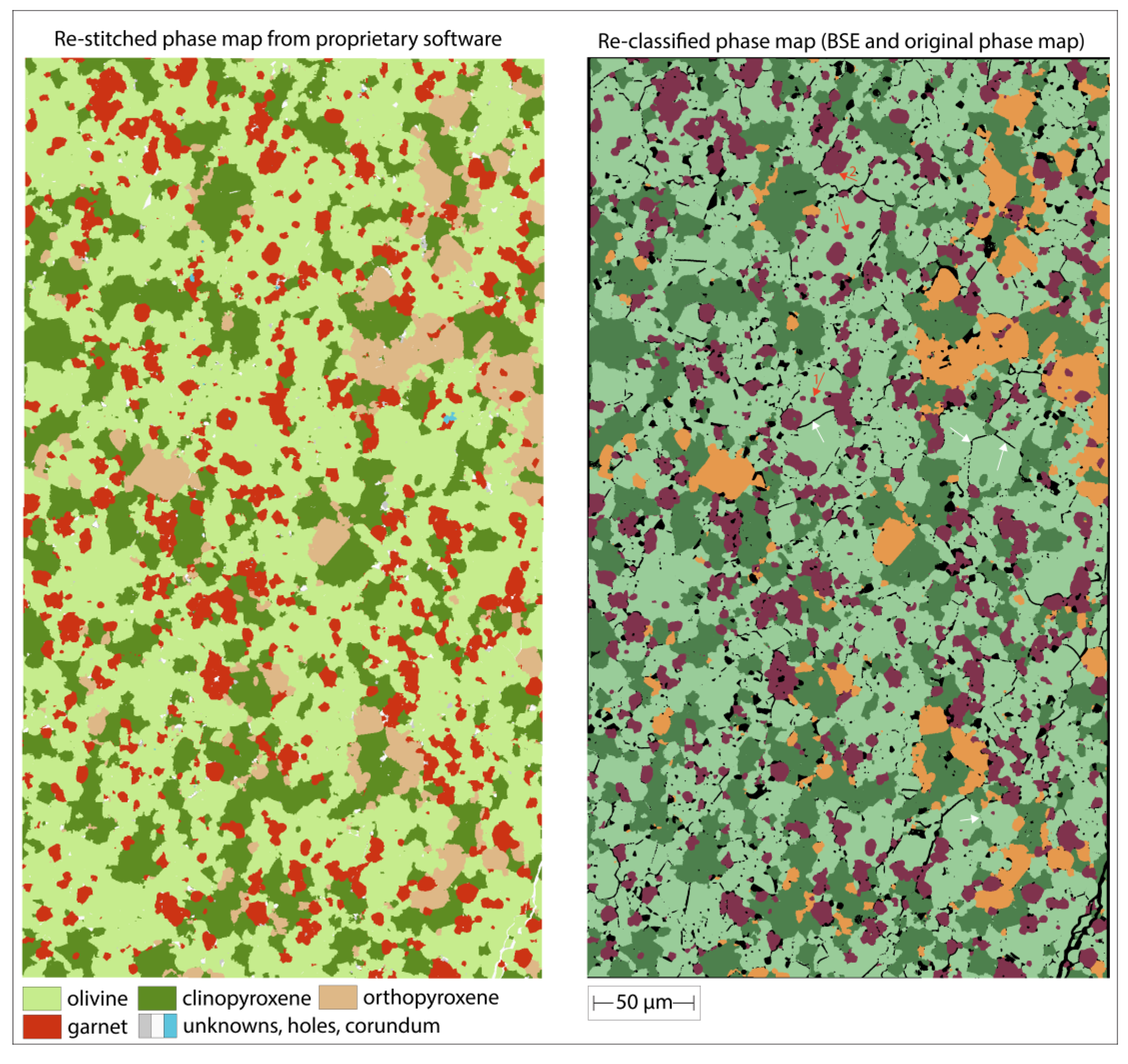
Figure 10.
The left panel shows re-registered phase map made with transformation matrix (intensity-based registration) from exported overlapping Bruker AMICS BSE frames applied to exported phase map frames. The right panel shows new phase map generated with annotations in QuPath on combined Bruker AMICS BSE and phase maps. The color scheme follows Figure 3. Note the better definition of grain boundaries of the same phase (white arrows) on the right-hand side phase map as well as the better distinction between included and adjacent phases (red arrows highlighting garnet-olivine relationships).
Beyond applications to experimental charges, the user-driven phase mapping open- source software workflow proposed here likely also has applications for petrographic thin sections. In most academic research projects, the investigator will have spent considerable time and effort inspecting the sample with a petrographic microscope before progressing to the SEM-EDS. Through optical microscopy, the investigator will thus have established the mineralogy of the rock forming phases as well as identified most of the accessory phases, unless the sample is very fine-grained or mineralogically very complex. This knowledge is pre-requisite for annotating and training the pixel classifier in our open-source workflow. The additional information from EDS spectra on rare or very finely grained accessory phases can then be used to identify the phases for which optical mineralogy did not yield conclusive answers. Thus, a user-driven approach is more likely to avoid erroneous misidentification of phases from a generic SEM-EDS spectral library. Such misattributions could, for example, arise from EDS spectral artefacts or from combining unrelated spectra of low integrated signals from adjacent unrelated pixel groups.
One final difference between instrument software generated phase maps and the user annotated workflow presented here concerns boundaries between grains of the same phase. For such comparison, we re-registered an instrument generated phase map to correct for the small x-y offsets shown in Figure 9. This resulted in improved stitching (Figure 10a) but the classified mineral pixels yielded a phase map that looks ‘flatter’ than the microstructure of experimental charge. When the same phase map was stacked with the original BSE layer and then annotated in QuPath (Figure 10b), the resulting phase proportions expectedly remained unchanged, but the microstructure appeared more realistic. Namely, the monolithic background of olivine in Figure 10a is broken up into subgrains, separated by narrow boundaries of pixels attributed to ‘holes’ (Figure 10b, white arrows). With a clearer appreciation of subgrains, it is also easier to identify included minerals versus interstitial grains (red arrows on Figure 10b). The improved representation of microstructure stems from a combination of factors. First, we used the BSE layer in QuPath to define the annotations. It contains much more structural detail than the EDS element maps that underpin the instrument-generated phase map. Second, we carefully applied the brush and wand tool to classify pixels to the exact edge of grains or subgrains. Third, we used classification trainers at high pixel resolution.
Notwithstanding the utility of pixel-based classification for obtaining modal abundance and determining association matrices (Figure 5–7), a true analysis of micro-structure requires grouping all pixels of a single grain into an object. This information yields additional insight into mutual contact relationships of actual mineral grains and sub-grains as well as melt films and pockets (where present). Namely, even though the microstructure of the pixel-classified phase map on Figure 10b looks realistic, it contains no actual information about which pixels belong to individual grains, for example, of olivine. Merging of pixels belonging to one object requires additional crystallographic information, typically obtained with electron-back-scattered-diffraction (EBSD) [39] or multi-angle cross-polarized light microscopy [40]. Only with such information is deeper analysis of mineral and melt fabrics possible, for example, to establish crystal preferred orientation, topotaxic growth or eutectic crystallization e.g., [41]. Thus, additional data layers (e.g. EBSD) may further benefit phase mapping of experimental charges.
Other additional data layers that could be integrated with phase maps are trace element maps obtained with high spatial resolution instruments. Due to the fine-grained nature of high PT experimental charges, it is difficult to obtain low-detection limit analysis for trace elements from conventional spot analysis, for example, with laser ablation. Full trace element maps have already been shown to yield improved trace element partitioning between melts and solids in high PT charges [42]. When combined with phase maps, all pixel locations of a phase can be pooled and their collective trace element signal can be quantified to obtain lower detection limits e.g., [43], opening the prospect of better partition coefficients for trace elements that are in low abundance.
5. Summary
This study explored the utility of phase maps for characterization of high PT experimental charges, with the following summarized findings:
- Due to their small sizes, it is feasible to obtain high quality BSE and EDS imagery for high PT experimental charges, requiring reasonable SEM instrument time (ca. 3 hours). This effort is modest in relation to the production of the experiment and analysis of phase chemistry on the EMPA.
- Phase maps of experimental charges give readers more tangible and complete evidence of phase equilibrium and phase relations than microphotographs of representative areas alone.
- Phase maps generated with commercial automated mineralogy software are suitable to document phase relationships within charges, constrain modes, test for equilibrium, and identify EMPA analysis targets.
- For charges with phases in low abundance, user-assisted phase mapping holds greater promise for obtaining accurate modal abundance estimates than those generated with current proprietary software.
- In the studied sub-solidus charge, the system chemistry calculated from the phase map corresponded very well with the nominal chemistry and demonstrated closed system.
- Mutual pixel neighborhood relationships (quantified as association indices) can be used to verify the plausibility of mass balance-derived reaction equations.
- Phase maps have the potential to add retrospective additional value to historic experimental charges.
- In the future, when combined with high spatial resolution trace element geochemical maps, phase maps have potential to improve counting statistics for low abundance trace elements.
Author Contributions
Conceptualization, B.S.K. and M.A.A.Z.; methodology, M.L., M.N. and M.A.A.Z.; software, M.A.A.Z.; validation, M.L. and M.N.; formal analysis, all; investigation, R.F.R.; writing—original draft preparation, B.S.K., R.F.R., and M.A.A.Z.; writing—review and editing, all; visualization, M.A.A.Z., B.S.K., and R.F.R.; supervision, G.M.Y. and B.S.K.; project administration, B.S.K. and G.M.Y.; funding acquisition, B.S.K. and G.M.Y. All authors have read and agreed to the published version of the manuscript.
Funding
This research was funded by the Australian Research Council, grant number DP220100136. R.F.R. received an international student Research Training Program PhD scholarship from the Australian Government.
Data Availability Statement
The full input images, intermediate files (images and metadata), and output phase maps are provided as QuPath projects (https://zenodo.org/records/14822997). The workflow to re-stitch AMICS software image tiles can be found as a commented script ‘imageJ_stack_matthew_v3.py’.
Acknowledgments
We acknowledge David Clark’s assistance in the high-pressure experimental petrology laboratories at ANU. EMPA analyses were supported by the Centre for Advanced Microscopy, an advanced imaging facility under Microscopy Australia, funded by the Australian National University and Australian State and Federal Governments. We thank Jeff Chen, Frank Brink, Corinne Frigo and Eric Lochner for their assistance with quantitative WDS analyses of these experiments. We thank Eligiusz Gugula for technical input on phase mapping. NewSpec Pty Ltd, Hitachi High-Tech, Bruker and The University of Queensland Centre for Microscopy and Microanalysis are thanked for access to Hitachi SU7000 FE-SEM with Bruker EDS detectors and AMICS software.
Conflicts of Interest
The authors declare no conflicts of interest.
References
- Walter, M.J., 1998. Melting of garnet peridotite and the origin of komatiite and depleted lithosphere. Journal of petrology, 39(1), pp.29-60. [CrossRef]
- Canil, D., 1991. Experimental evidence for the exsolution of cratonic peridotite from high-temperature harzburgite. Earth and Planetary Science Letters, 106(1-4), pp.64-72. [CrossRef]
- Takahashi, E., Shimazaki, T., Tsuzaki, Y. and Yoshida, H., 1993. Melting study of a peridotite KLB-1 to 6.5 GPa, and the origin of basaltic magmas. Philosophical Transactions of the Royal Society of London. Series A: Physical and Engineering Sciences, 342(1663), pp.105-120. [CrossRef]
- Eggler, D.H., 1979. Experimental igneous petrology. Reviews of Geophysics, 17(4), pp.744-761. [CrossRef]
- Green, T.H., 1980. Island arc and continent-building magmatism—A review of petrogenic models based on experimental petrology and geochemistry. Tectonophysics, 63(1-4), pp.367-385. [CrossRef]
- Newton, R.C. and Manning, C.E., 2010. Role of saline fluids in deep-crustal and upper-mantle metasomatism: insights from experimental studies. Geofluids, 10(1-2), pp.58-72. [CrossRef]
- Ezad, I.S., Blanks, D.E., Foley, S.F., Holwell, D.A., Bennett, J. and Fiorentini, M.L., 2024. Lithospheric hydrous pyroxenites control localisation and Ni endowment of magmatic sulfide deposits. Mineralium Deposita, 59(2), pp.227-236. [CrossRef]
- Ezad, I.S., Saunders, M., Shcheka, S.S., Fiorentini, M.L., Gorojovsky, L.R., Förster, M.W. and Foley, S.F., 2024. Incipient carbonate melting drives metal and sulfur mobilization in the mantle. Science Advances, 10(12), p.eadk5979. [CrossRef]
- Song, W., Xu, C., Veksler, I.V. and Kynicky, J., 2016. Experimental study of REE, Ba, Sr, Mo and W partitioning between carbonatitic melt and aqueous fluid with implications for rare metal mineralization. Contributions to Mineralogy and Petrology, 171, pp.1-12. [CrossRef]
- London, D., 1992. The application of experimental petrology to the genesis and crystallization of granitic pegmatites. The Canadian Mineralogist, 30(3), pp.499-540.
- Brey, G.P. and Köhler, T., 1990. Geothermobarometry in four-phase lherzolites II. New thermobarometers, and practical assessment of existing thermobarometers. Journal of Petrology, 31(6), pp.1353-1378.
- Nickel, K.G. and Green, D.H., 1985. Empirical geothermobarometry for garnet peridotites and implications for the nature of the lithosphere, kimberlites and diamonds. Earth and Planetary Science Letters, 73(1), pp.158-170. [CrossRef]
- Sudholz, Z.J., Yaxley, G.M., Jaques, A.L. and Brey, G.P., 2021. Experimental recalibration of the Cr-in-clinopyroxene geobarometer: improved precision and reliability above 4.5 GPa. Contributions to Mineralogy and Petrology, 176, pp.1-20. [CrossRef]
- Albarede, F. and Provost, A., 1977. Petrological and geochemical mass-balance equations: an algorithm for least-square fitting and general error analysis. Computers & Geosciences, 3(2), pp.309-326. [CrossRef]
- Pertermann, Maik, and Marc M. Hirschmann. "Partial melting experiments on a MORB-like pyroxenite between 2 and 3 GPa: Constraints on the presence of pyroxenite in basalt source regions from solidus location and melting rate." Journal of Geophysical Research: Solid Earth 108, no. B2 (2003). [CrossRef]
- Schulz, B., Sandmann, D. and Gilbricht, S., 2020. SEM-based automated mineralogy and its application in geo-and material sciences. Minerals, 10(11), p.1004. [CrossRef]
- Hrstka, T., Gottlieb, P., Skala, R., Breiter, K. and Motl, D., 2018. Automated mineralogy and petrology-applications of TESCAN Integrated Mineral Analyzer (TIMA). Journal of Geosciences, 63(1), pp.47-63. [CrossRef]
- Farmer, N. and O'Neill, H.S.C., 2024. The use of MgO–ZnO ceramics to record pressure and temperature conditions in the piston–cylinder apparatus. European Journal of Mineralogy, 36(3), pp.473-489.
- Riel, N., Kaus, B.J., Green, E.C.R. and Berlie, N., 2022. MAGEMin, an efficient Gibbs energy minimizer: application to igneous systems. Geochemistry, Geophysics, Geosystems, 23(7), p.e2022GC010427. [CrossRef]
- Holland, T.J., Green, E.C. and Powell, R., 2018. Melting of peridotites through to granites: a simple thermodynamic model in the system KNCFMASHTOCr. Journal of Petrology, 59(5), pp.881-900. [CrossRef]
- Cardona, A., Saalfeld, S., Schindelin, J., Arganda-Carreras, I., Preibisch, S., Longair, M., Tomancak, P., Hartenstein, V. and Douglas, R.J., 2012. TrakEM2 software for neural circuit reconstruction. PloS one, 7(6), p.e38011. [CrossRef]
- Bogovic, J.A., Hanslovsky, P., Wong, A. and Saalfeld, S., 2016, April. Robust registration of calcium images by learned contrast synthesis. In 2016 IEEE 13th international symposium on biomedical imaging (ISBI) (pp. 1123-1126). IEEE.
- Schindelin, J., Arganda-Carreras, I., Frise, E., Kaynig, V., Longair, M., Pietzsch, T., Preibisch, S., Rueden, C., Saalfeld, S., Schmid, B. and Tinevez, J.Y., 2012. Fiji: an open-source platform for biological-image analysis. Nature methods, 9(7), pp.676-682. [CrossRef]
- Bankhead, P., Loughrey, M.B., Fernández, J.A., Dombrowski, Y., McArt, D.G., Dunne, P.D., McQuaid, S., Gray, R.T., Murray, L.J., Coleman, H.G. and James, J.A., 2017. QuPath: Open source software for digital pathology image analysis. Scientific reports, 7(1), pp.1-7. [CrossRef]
- Chiaruttini, N., Burri, O., Haub, P., Guiet, R., Sordet-Dessimoz, J. and Seitz, A., 2022. An open-source whole slide image registration workflow at cellular precision using Fiji, QuPath and Elastix. Frontiers in Computer Science, 3, p.780026. [CrossRef]
- Acevedo Zamora, M.A. and Kamber, B.S., 2023. Petrographic microscopy with ray tracing and segmentation from multi-angle polarisation whole-slide images. Minerals, 13(2), p.156. [CrossRef]
- Koch, P.H., 2017. Particle generation for geometallurgical process modeling (Doctoral dissertation, Luleå tekniska universitet).
- Kim, J.J., Ling, F.T., Plattenberger, D.A., Clarens, A.F. and Peters, C.A., 2022. Quantification of mineral reactivity using machine learning interpretation of micro-XRF data. Applied Geochemistry, 136, p.105162. [CrossRef]
- Tomlinson, E.L. and Kamber, B.S., 2021. Depth-dependent peridotite-melt interaction and the origin of variable silica in the cratonic mantle. Nature Communications, 12(1), p.1082. [CrossRef]
- Walter, M.J., Sisson, T.W. and Presnall, D.C., 1995. A mass proportion method for calculating melting reactions and application to melting of model upper mantle lherzolite. Earth and Planetary Science Letters, 135(1-4), pp.77-90. [CrossRef]
- Pertermann, M. and Hirschmann, M.M., 2003. Anhydrous partial melting experiments on MORB-like eclogite: phase relations, phase compositions and mineral–melt partitioning of major elements at 2–3 GPa. Journal of Petrology, 44(12), pp.2173-2201.
- Lund, C., Lamberg, P. and Lindberg, T., 2015. Development of a geometallurgical framework to quantify mineral textures for process prediction. Minerals engineering, 82, pp.61-77. [CrossRef]
- Lanari, P. and Engi, M., 2017. Local bulk composition effects on metamorphic mineral assemblages. Reviews in Mineralogy and Geochemistry, 83(1), pp.55-102. [CrossRef]
- Tomlinson, E.L. and Holland, T.J., 2021. A thermodynamic model for the subsolidus evolution and melting of peridotite. Journal of Petrology, 62(1), p.egab012. [CrossRef]
- Lesher, C.E., Pickering-Witter, J., Baxter, G. and Walter, M., 2003. Melting of garnet peridotite: Effects of capsules and thermocouples, and implications for the high-pressure mantle solidus. American Mineralogist, 88(8-9), pp.1181-1189. [CrossRef]
- Ali, A., Zhang, N. and Santos, R.M., 2023. Mineral characterization using scanning electron microscopy (SEM): a review of the fundamentals, advancements, and research directions. Applied Sciences, 13(23), p.12600. [CrossRef]
- Acevedo Zamora, M.A.A., Caulfield, J.T., Laupland, E., Kamber, B.S. and Allen, C.M., 2025, January. Mineral Separate Microanalysis with Intelligent Spot Placement, Manual Edition, and Simulation: Two Correlative Microscopy Prototypes for Relating Zircon Texture, Age, and Geochemistry. In 13th Asia Pacific Microscopy Congress 2025 (APMC13) (p. 280). ScienceOpen.
- Ogliore, R.C., 2021. Acquisition and Online Display of High-Resolution Backscattered Electron and X-Ray Maps of Meteorite Sections. Earth and Space Science, 8(7), p.e2021EA001747. [CrossRef]
- Nowell, M.M. and Wright, S.I., 2004. Phase differentiation via combined EBSD and XEDS. Journal of microscopy, 213(3), pp.296-305. [CrossRef]
- Acevedo Zamora, M.A., Schrank, C.E. and Kamber, B.S., 2024. Using the traditional microscope for mineral grain orientation determination: A prototype image analysis pipeline for optic-axis mapping (POAM). Journal of Microscopy. [CrossRef]
- Xu, H., Zhang, J., Yu, T., Rivers, M., Wang, Y. and Zhao, S., 2015. Crystallographic evidence for simultaneous growth in graphic granite. Gondwana Research, 27(4), pp.1550-1559. [CrossRef]
- Bussweiler, Y., Gervasoni, F., Rittner, M., Berndt, J. and Klemme, S., 2020. Trace element mapping of high-pressure, high-temperature experimental samples with laser ablation ICP time-of-flight mass spectrometry–Illuminating melt-rock reactions in the lithospheric mantle. Lithos, 352, p.105282.
- Acevedo Zamora, M.A.A., Kamber, B.S., Jones, M.W., Schrank, C.E., Ryan, C.G., Howard, D.L., Paterson, D.J., Ubide, T. and Murphy, D.T., 2024. Tracking element-mineral associations with unsupervised learning and dimensionality reduction in chemical and optical image stacks of thin sections. Chemical Geology, 650, p.121997. [CrossRef]
Figure 1.
Details extracted from BSE frames obtained on sample UHP32, exposing olivine, clinopyroxene, garnet and orthopyroxene. The 8 images were obtained with increasingly slow scan speeds (S3 to S10, reflecting 1, 3.2, 10, 32, 100, 320, 1000, and 3200 μs/pixel). Note that grain boundaries are becoming substantially clearer from S5 to S8, but that further improvement from S8 to S10 relates to diminishing greyscale ‘noise’ within phases rather than sharpness of grain contacts. Also shown for comparison is a phase map (bottom right corner).
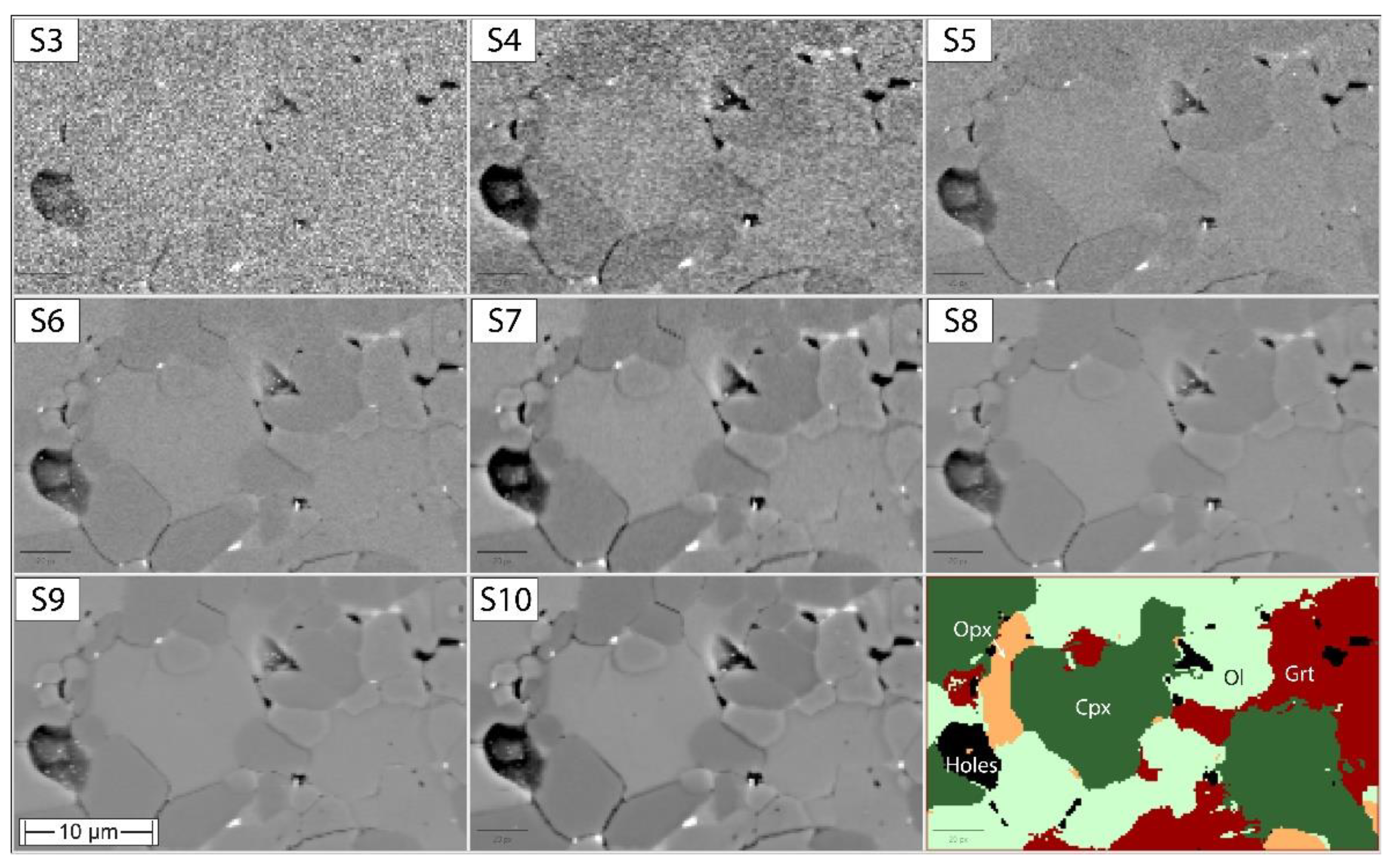
Figure 2.
BSE intensity profiles (16-bit) across orthopyroxene, garnet, olivine and clinopyroxene peridotite assemblage of UHP32, shown as a phase map on the top panel. In all BSE intensity profiles, the scan speed setting of interest (red traces S6, S7, S8 and S9) was compared to the slowest speed setting S10 (as a grey line).
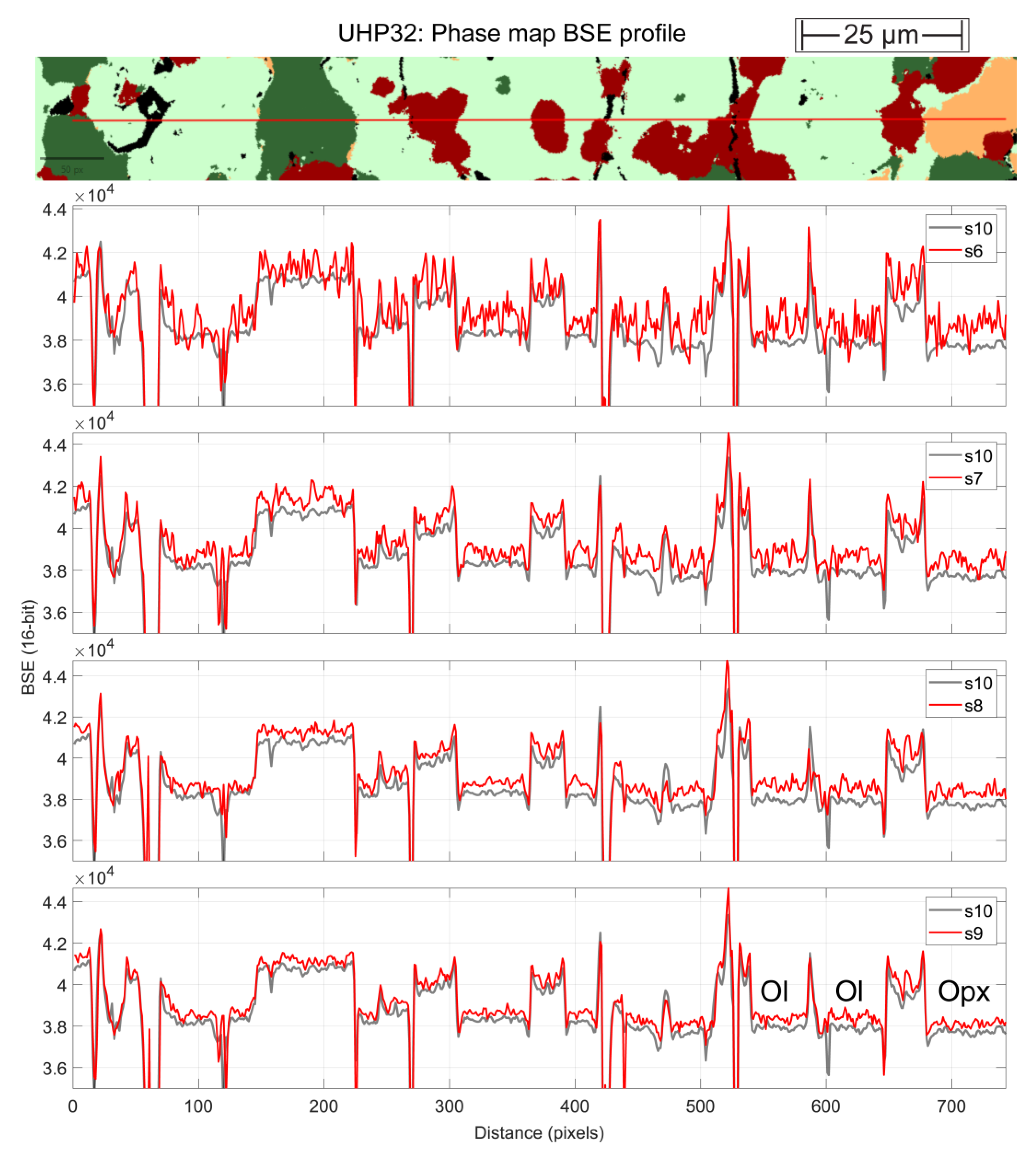
Figure 3.
Small area phase maps on sample UHP32. (a) was obtained with the proprietary TIMA software combining fast BSE scanning with high-resolution EDS mapping. (b) was obtained with the open-source software approach developed for this study combining the slowest scan speed (S10) BSE image with high-resolution EDS mapping. The areas shown in Figure 1 and Figure 2 are indicated with open grey boxes. (c) and (d) both used BSE images obtained with scan speed S7 but were combined with high-resolution (c) and dot mapping (d) EDS acquisitions.
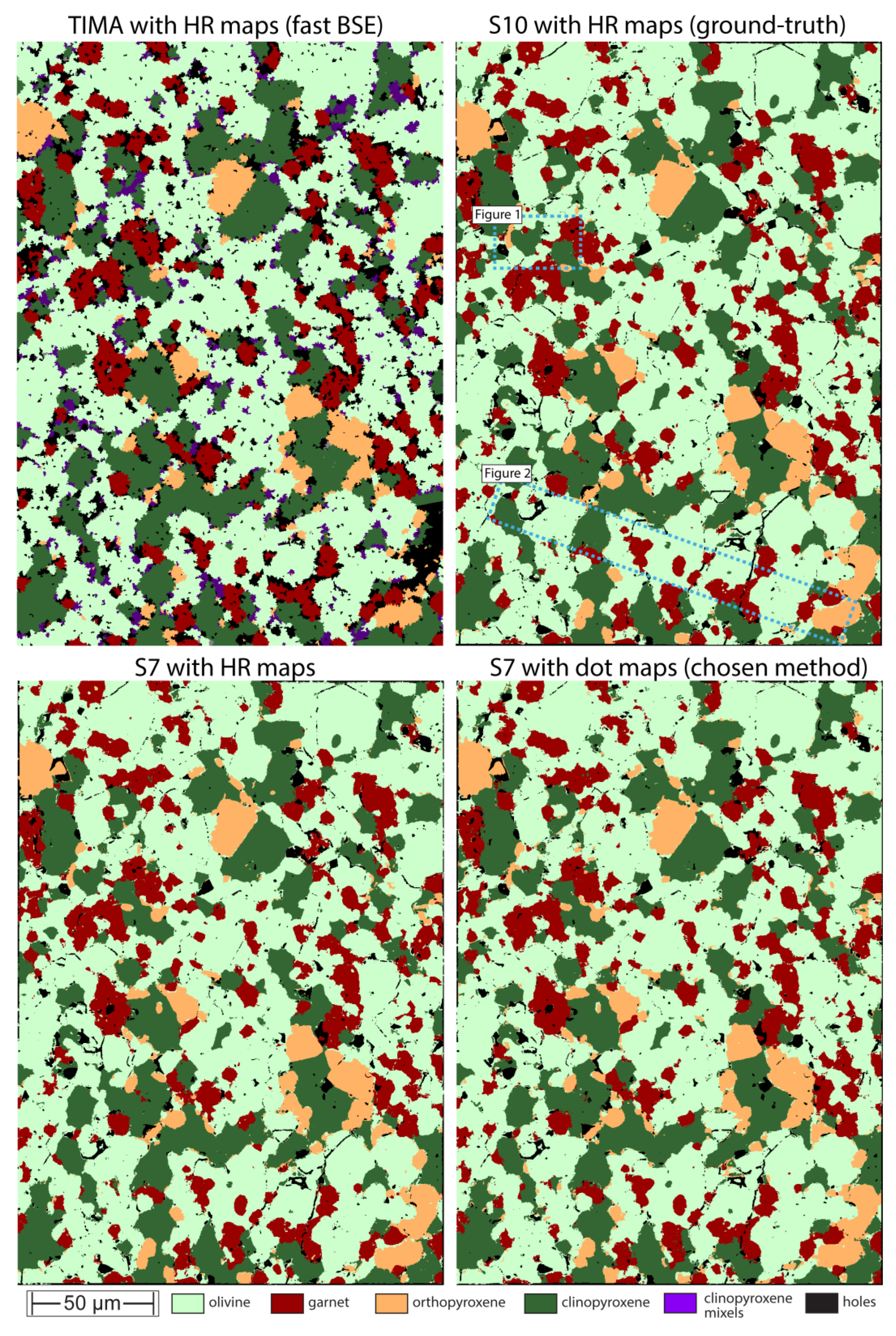
Figure 4.
Linear regressions of various estimates of modal abundance (all by wt%). Panels (a) and (b) use data for small trial area on sample UHP32 (see Figure 3). Both panels show the ground-truth BSE S10 with high-resolution EDS (Figure 3b) on the x-axis and faster acquisitions on the y-axes. Panel (c) shows modal abundance estimates for the full charge area for samples UHP32 (see Figure 5 for full phase map) and UHP41 (see Figure 6 for full phase map). The x-axis shows mode by mass balance and the y-axis mode by phase map (BSE S7 with EDS dot mapping).
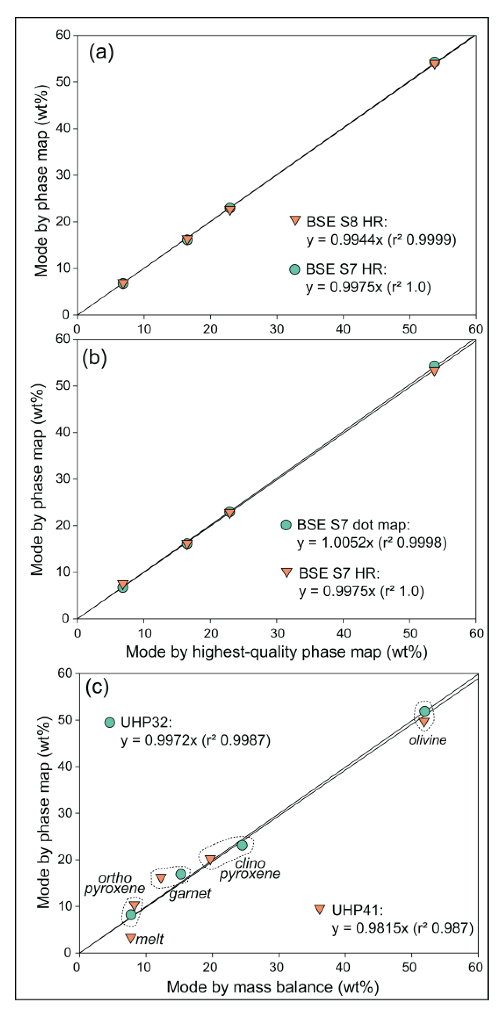
Figure 5.
Modes, phase associations and phase map of sample UHP32. (a) and (b) show mode and mutual phase associations in ‘Zone A’ and ‘Zone B’, respectively, of the phase map (c). Same color scheme as Figure 3.
Figure 5.
Modes, phase associations and phase map of sample UHP32. (a) and (b) show mode and mutual phase associations in ‘Zone A’ and ‘Zone B’, respectively, of the phase map (c). Same color scheme as Figure 3.
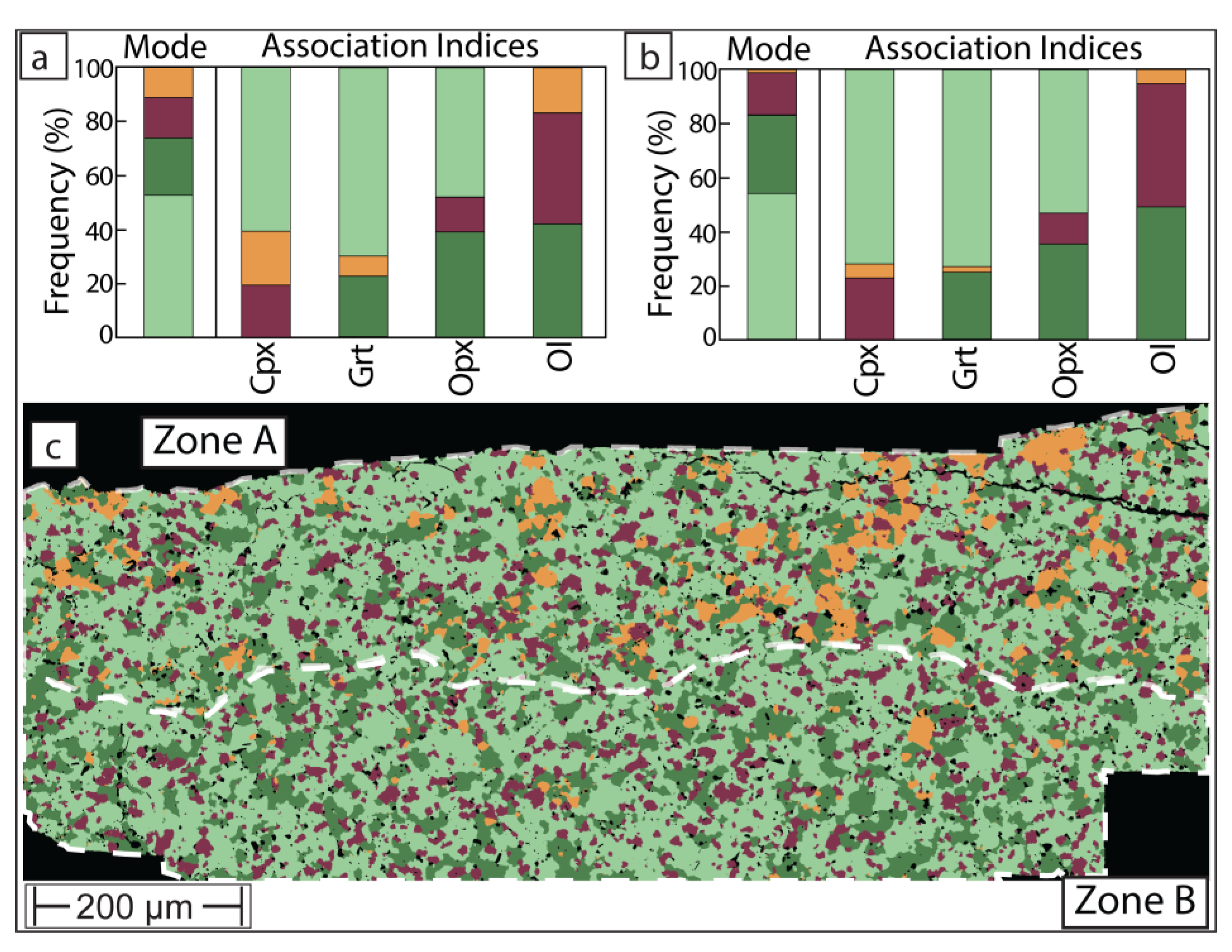
Figure 6.
Modes, phase associations and phase map of sample UHP40. (a) and (b) show mode and mutual phase associations in ‘Zone A’ and ‘Zone B’, respectively, of the phase map (c). Minerals shown in same color scheme as Figure 3 with the addition of melt in rose red.
Figure 6.
Modes, phase associations and phase map of sample UHP40. (a) and (b) show mode and mutual phase associations in ‘Zone A’ and ‘Zone B’, respectively, of the phase map (c). Minerals shown in same color scheme as Figure 3 with the addition of melt in rose red.
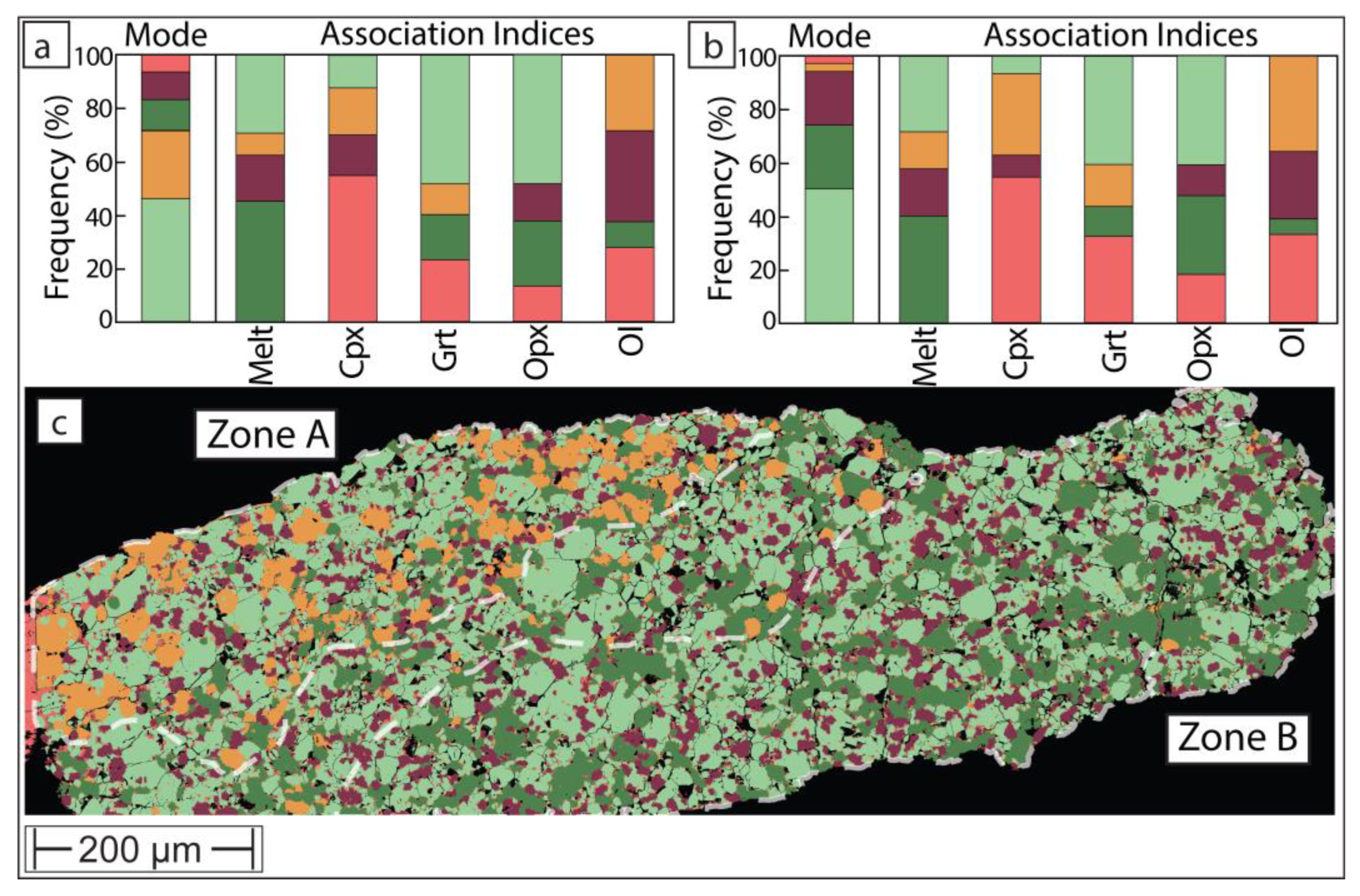
Figure 8.
Thermodynamically modelled wt% modal abundance of pyroxenes and garnet in GKR-001. The x-axis shows melt fraction (wt%) generated over 23°C and the y-axis shows modal abundance of minerals in the solid residue (olivine not shown). Over a very narrow temperature interval of 16°C, this system is modelled to produce 16.6 wt% melt (x-axis) at the expense of clinopyroxene, while also crystallizing copious peritectic orthopyroxene.
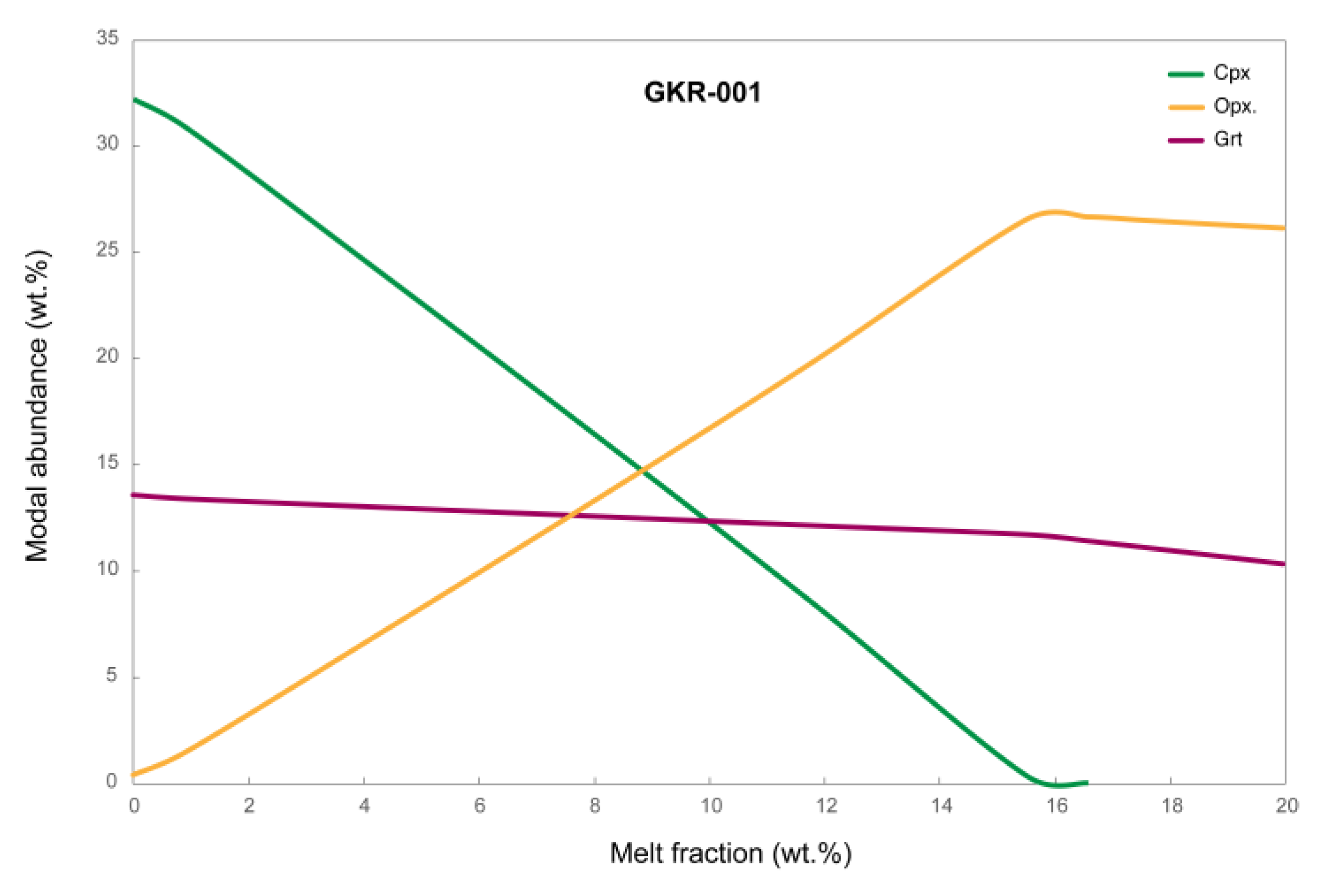

Table 1.
Composition of the starting mixture (GKR-001) and run products.
| GKR-001 | UHP32 | ||||
| Ol (32)2 | Opx (17) | Cpx (30) | Grt (23) | ||
| SiO2 | 45.52 | 40.83 (23)3 | 56.36 (22) | 55.03 (23) | 42.37 (28) |
| TiO2 | 0.07 | 0.08 (06) | 0.04 (01) | 0.04 (01) | 0.21 (07) |
| Al2O3 | 4.41 | 0.17 (20) | 2.55 (17) | 2.67 (09) | 22.70 (60) |
| Cr2O3 | 0.32 | 0.09 (02) | 0.28 (02) | 0.30 (03) | 1.29 (23) |
| FeOt | 7.11 | 8.80 (16) | 5.18 (08) | 4.57 (15) | 5.66 (16) |
| MnO | 0.15 | 0.14 (01) | 0.13 (02) | 0.15 (02) | 0.21 (03) |
| MgO | 38.18 | 49.97 (37) | 33.15 (59) | 25.50 (31) | 22.48 (20) |
| NiO | 0.10 | 0.08 (03) | 0.06 (02) | 0.05 (01) | bdl |
| CaO | 3.96 | 0.30 (15) | 2.62 (68) | 11.53 (43) | 5.07 (26) |
| Na2O | 0.09 | 0.03 (00) | 0.07 (02) | 0.24 (01) | bdl |
| K2O | 0.01 | bdl1 | bdl | bdl | bdl |
| Total | 99.90 | 100.39 | 100.40 | 100.05 | 99.99 |
| Mg# | 90.54 | 91.01 | 91.94 | 90.87 | 90.76 |
| Mode (wt.%) Mass balance Phase map |
|
51.95 51.87 |
7.74 8.19 |
24.48 23.07 |
15.23 16.86 |
| UHP40 | |||||
| Ol (22) | Opx (29) | Cpx (29) | Grt (27) | Melt (07)4 | |
| SiO2 | 41.10 (22) | 56.12 (43) | 54.74 (26) | 42.85 (23) | 46.74 (97) |
| TiO2 | bdl | 0.03 (01) | 0.03 (01) | 0.15 (03) | 0.24 (07) |
| Al2O3 | 0.15 (02) | 3.11 (34) | 3.12 (12) | 22.71 (36) | 8.90 (1.0) |
| Cr2O3 | 0.10 (01) | 0.32 (03) | 0.35 (02) | 1.36 (22) | 0.44 (04) |
| FeOt | 8.21 (13) | 4.93 (09) | 4.56 (14) | 5.22 (16) | 11.11 (02) |
| MnO | 0.13 (01) | 0.12 (01) | 0.15 (01) | 0.20 (02) | 0.17 (01) |
| MgO | 50.24 (28) | 32.98 (32) | 26.74 (56) | 22.71 (24) | 18.00 (1.2) |
| NiO | 0.02 (01) | 0.03 (01) | 0.02 (00) | bdl | bdl |
| CaO | 0.28 (01) | 2.56 (18) | 9.79 (69) | 4.95 (22) | 13.95 (07) |
| Na2O | 0.02 (01) | 0.07 (01) | 0.21 (02) | bdl | 0.45 (02) |
| K2O | bdl | bdl | bdl | bdl | 0.01 (00) |
| Total | 100.32 | 100.24 | 99.69 | 100.15 | 100.00 |
| Mg# | 91.50 | 92.26 | 91.27 | 90.27 | 74.27 |
| Mode (wt.%) Mass balance Phase map |
51.84 49.78 |
8.24 10.37 |
19.66 20.22 |
12.23 16.24 |
7.69 3.38 |
1 bdl = below detection limit. 2 Number of analyses. 3 Standard deviation of “n” analyses of each phase in each experimental run product. 4 Melt composition was normalized to 100 %.
Disclaimer/Publisher’s Note: The statements, opinions and data contained in all publications are solely those of the individual author(s) and contributor(s) and not of MDPI and/or the editor(s). MDPI and/or the editor(s) disclaim responsibility for any injury to people or property resulting from any ideas, methods, instructions or products referred to in the content. |
© 2025 by the authors. Licensee MDPI, Basel, Switzerland. This article is an open access article distributed under the terms and conditions of the Creative Commons Attribution (CC BY) license (http://creativecommons.org/licenses/by/4.0/).
Copyright: This open access article is published under a Creative Commons CC BY 4.0 license, which permit the free download, distribution, and reuse, provided that the author and preprint are cited in any reuse.


