
Submitted:
11 February 2025
Posted:
12 February 2025
You are already at the latest version
Abstract
Comprehensive investigations were conducted on numerical methods for simulating high–pressure water jet in air impacting on a flat plate. The primary focus was on the influence of numerical methods on the impact pressure exerted on the flat plate. Taking into account the principal characteristics of high–pressure water jets in air, the Eulerian multiphase model was selected as the foundational approach for simulating multiphase flows. Firstly, two turbulence treatment methods were investigated, revealing that the mixture turbulence model method yields superior results compared to the per–phase turbulence model method. Subsequently, the effects of turbulence models on the impact pressure were examined. Two two–equation turbulence models (the realizable k–ε model and the SST k–ω model), widely employed in engineering, and a four–equation turbulence model (the SST k–ω–φ–α model) were comparatively analyzed. It was observed that the SST k–ω–φ–α model yields more accurate results in the vicinity of the stagnation point. The influences of the inlet boundary condition were also explored. It was determined that the inlet turbulence condition derived from a hydraulic diameter–based empirical formula, as provided in the commercial CFD software ANSYS Fluent, is unsuitable for numerical simulations of high–pressure water jets in air. Subsequently, the influence of bubble diameters in the secondary phase (air) was scrutinized. Results indicated that as the bubble diameter diminishes, the impact pressure likewise decreases. However, once the bubble diameter reaches a certain size, it exerts almost no effect on the impact pressure. Finally, it was also verified that surface tension has no effect on the impact pressure of high–pressure water jets in air when the nozzle exit is not so far from the flat plate.
Keywords:
numerical simulation
; high–pressure
; water jet
; turbulence model
; impact pressure
1. Introduction
High–pressure water jets have been successfully applied in various fields such as rock breaking[1], coal mining[2], vessel cleaning[3], machining and cutting[4], among others. In these engineering applications, the primary advantage lies in the high impacting pressure generated by high–pressure water jets on target objects, without inducing adverse factors such as high temperature, sparks, dust, and fragment splashing. Gaining an understanding of the characteristics of high–pressure water jets in air can facilitate their more effective utilization.
Leu et al. [5] conducted an analysis of the anatomy of high–pressure water jets in air, dividing the entire jet into three distinct regions: the initial (potential core), main (water droplet), and final (diffused droplet) regions. Jiang et al. [6] captured the entire structure of the high–pressure water jet flow instantaneously using a high–speed camera. They analyzed the overall morphology and velocity characteristics, subsequently reclassifying the flow structure from the conventional three regions into five regions: the potential core region, stripped droplet region, primary shear region, secondary shear region, and diffused droplet region. The principal characteristic of high–pressure water jets in air is that, under the strong action of shear stress at the interface, the flow structure gradually transforms from a continuous jet to a discrete flow dominated by droplets. During this process, due to momentum exchange between water and air, the water is decelerated while the air is accelerated. Rajaratnam et al. [7] investigated the flow field of very high velocity water jets in air using LDA (Laser Doppler Anemometry). They found that the velocity at the centerline of the jet remains approximately constant at U0 (inlet velocity) within an axial distance from the nozzle of about 100D (where D is the nozzle diameter), and then decreases continuously to about 0.25U0 at an axial distance of 2500D. Rajaratnam et al. [8] also measured the water distribution along the axis of high–velocity jets. Their measurements revealed that the water concentration on the axis of the jet decreased rapidly with the axial distance, falling to about 5% at 100D and 2% at 200D. It is evident that, due to the significantly lower density of air compared to water, a high degree of air entrainment into the jet will dramatically reduce the jet's kinetic energy, despite the air having the same velocity as the water phase. Furthermore, the impact pressure on the plate, which results from the transformation of the jet's kinetic energy, will inevitably decrease significantly. From an application perspective, the pressure distribution on the plate is the most critical aspect. Therefore, greater attention should be directed towards scenarios where the nozzle is not too far from the targets.
Experiment is a commonly employed method for investigating the characteristics of high–pressure water jets. Leach et al. [9] investigated the overall characteristics of high–pressure water jets using short–exposure optical photography and X–ray photography. They also measured the distribution of impact pressure on a flat plate and analyzed it theoretically. In their experiments, the distance from the nozzle exit to the flat plate was 76D. Additionally, the effect of nozzle shape was also examined in detail. Guha et al. [10] conducted experimental studies on the pressure distribution on a flat plate (with the distance from the nozzle exit to the flat plate being 43D) for the purpose of designing an efficient cleaning system. They measured the pressure distributions and found that the pressure along the radial direction can be expressed by a Gaussian distribution. Moreover, the stagnation pressure on the flat plate decreases linearly with axial distance.
Numerical simulation is another widely used method by many researchers to investigate the characteristics of high–pressure water jets. Liu et al. [11] employed the multiphase volume of fluid (VOF) method in conjunction with the standard k–ε turbulence model to simulate the dynamic characteristics of an abrasive jet from a very fine nozzle. Guha et al. [10,12] conducted a simulation for high–pressure water jet flow using the Eulerian multiphase model in combination with the standard k–ε turbulence model and standard wall functions. By introducing a novel model for mass and momentum transfer, they achieved favorable results compared to the experimental findings of Leach et al. [9]. Liu et al. [13] comparatively investigated the impingement capability of high–pressure submerged and non–submerged water jets using the renormalization group (RNG) k–ε turbulence model. They found that the velocity in the submerged water jet is significantly lower than that in the non–submerged water jet at the same nozzle pressure.
The flow of high–pressure water jets in air is complex. Numerical simulation involves multiple challenging issues, including the establishment of multiphase flow models, the selection of turbulence models, and the handling of turbulence in multiphase flows, among others. To the best of the authors' knowledge, there has been no specialized study on the details of numerical methods in numerical studies concerning high–pressure water jets. This work focuses on the impact pressure on a flat plate and comprehensively investigates the numerical methods for simulating high–pressure water jets in air. The model formulation and implementation are briefly described in the subsequent section. Subsequently, the results are presented and discussed. Some conclusions are presented in the final section.
2. Model Formulation and Implementation
The high–pressure water jet in air is a typical gas–liquid multiphase flow. There are three conventional models that can be used for the numerical simulation of gas–liquid multiphase flows: the volume of fluid (VOF) model, the mixture model, and the Eulerian multiphase model.
The VOF model is suitable for problems where the gas and liquid phases do not penetrate each other and have clear interfaces. Conversely, the mixture model is appropriate for flows in which the gas and liquid mix well. Evidently, the problem of a high–pressure water jet in air impacting on a flat plate does not fall into these two categories. The Eulerian multiphase model can solve complex multiphase flows and is a suitable choice for the problems we need to address in this work. When the Eulerian multiphase model is applied to isothermal, incompressible, viscous, and turbulent two–phase flows, its governing equations consist of the continuity equations, the momentum equations, and the turbulence transport equations.
The Eulerian multiphase model used in the ANSYS Fluent CFD package is constructed based on the following assumptions:
1. All phases share a single pressure.
2. The continuity equations and the momentum equations are solved for each phase.
3. The turbulence model can be applied to the mixture or for each phase.
For the flow of high–pressure water jets in air, there is no mass exchange among the phases. Large velocities result in high Reynolds number (Re) and Weber number (We), rendering the effects of surface tension and wall lubrication insignificant and thus negligible. Moreover, due to the relatively small distance from the nozzle exit to the target, the gravitational force is also excluded.
Based on the aforementioned assumptions and simplifications, the governing equations can be written as follows.
2.1. Continuity Equations
For phase q, the continuity equation takes
where , are the volume fraction, density and velocity of phase q, respectively.
2.2. Momentum Equations
The momentum equation for phase q can be written as
where P is the pressure, is the turbulent dispersion force, and is an interaction force between phase p and q. represents the stress–strain tensor of phase q and can be written as
in which and are the shear and bulk viscosity of phase q.
The interaction force between phase p and q is simply modeled as
here represents the interphase exchange coefficient of momentum. For gas–liquid flow, it can be modeled as the general form:
where and are the density and diameter of the bubbles or droplets of the secondary phase, p. is the interfacial area. f is the drag function. is the particulate relaxation time, which is defined as
Many definitions for the drag function are adopted by different researchers. In this work, the Schiller and Naumann model is used. In this model, the drag function is
where and are drag coefficient and relative Reynolds number, respectively. They are defined as
and
Several methods have been provided for calculating the interfacial area. In this work, the symmetric model is selected. The interfacial area is calculated as
2.3. Turbulence Dispersion Force
The turbulent dispersion force can be treated as an interfacial momentum force in the phase momentum equations ( in Eqn. 2). Alternatively, its effect can be modeled by introducing a turbulent diffusion term into the phase continuity equations. The continuity equation for phase q can be written as
where the turbulent dispersion term must satisfy the constraint of
The diffusion coefficient is estimated from the turbulent viscosity as
In this work, the adjustable parameter = 1.0.
2.4. Turbulence Models
In ANSYS Fluent, three methods are available for the treatment of turbulence within the Eulerian multiphase model: the mixture turbulence model method, the dispersed turbulence model method, and the per–phase turbulence model method.
In the mixture turbulence model method, different substances are treated as a single mixture, and turbulence quantities—such as turbulence kinetic energy, turbulence energy dissipation rate, and specific dissipation rate—are computed based on this mixture.
The density, molecular viscosity, and velocity vectors of the mixture are determined using the following equations:
For turbulence models, by substituting all quantities of single–phase flow with those of the mixture, the calculation methods and corresponding constants for each term in the turbulent transport equations for multiphase flow are completely consistent with those of single–phase flow. For instance, the turbulent transport equations for the SST k–ω–φ–α turbulence model are presented below. This turbulence model, an elliptic blending–based model previously developed by the author, has demonstrated a strong capability in simulating jet heat transfer.
Regarding the realizable k–ε turbulence model and the SST k–ω turbulence model, as they have already been described in detail elsewhere, they will not be elaborated upon here. Interested readers can refer to the ANSYS Fluent help documentation for further information.
The dispersed turbulence model method is applicable when there is clearly one primary continuous phase and the rest are dispersed, dilute secondary phases. In the flow of high–pressure water jets in air, this situation is clearly not met.
In the per–phase turbulence model method, a set of turbulence transport equations are solved for each phase. When turbulence transfer among phases plays a dominant role, it is an appropriate choice. For the flow of high–pressure water jets in air, the per–phase turbulence model method is feasible. However, due to the complex construction and lengthy description of this method, it will not be described in detail here. Those interested can refer to the help documentation of ANSYS Fluent.
2.5. Model implementation
The ANSYS Fluent CFD package was adopted as the computing platform. In the present work, three turbulence models, namely the realizable k–ε turbulence model, the SST k–ω turbulence model, and the SST k–ω–φ–α turbulence model, were used to simulate the high–pressure impinging water jet flow. The realizable k–ε model and the SST k–ω model are embedded models within ANSYS Fluent and can be directly utilized. The user–defined scalar (UDS) functionality of ANSYS Fluent was employed to implement the SST k–ω–φ–α model [14].
The governing equation system, which comprises the multiphase form of continuity equations, momentum equations, and turbulence transportation equations, was solved using a pressure–based coupled algorithm. The convection terms in the momentum equations and turbulence transportation equations were discretized using the second–order upwind scheme. The gradients and derivatives were evaluated using the least squares cell–based method.
3. Results and Discussion
3.1. Computational Model
The problem of a high–pressure water jet issuing from a circular nozzle and flowing in air, which vertically impinges on a flat plate, was simulated in the present work. The computational model was constructed based on the experiment conducted by Leach et al. [9], which was used to verify the numerical results. Considering the axisymmetric characteristics in both geometry and physics, the problem was simplified to an axisymmetric model. The schematic view of the model geometry and relevant boundary conditions is shown in Figure 1(a). Here, D = 1 mm represents the diameter of the inlet, which is also the diameter of the circular nozzle. L = 76D denotes the distance from the inlet (nozzle exit) to the flat plate. H = 25D indicates the lateral dimension of the computational region.
Numerous studies have demonstrated that the nozzle geometry significantly affects the jet flow [2,9,15]. In this work, as a precursor, the water flow within the nozzle was simulated, and the flow quantities at the nozzle outlet were extracted and applied to the inlet of the computational model. The nozzle geometry and relevant boundary conditions are shown in Figure 1(b).
Different wall treatment methods were employed for various turbulence models. Specifically, for the SST k–ω–φ–α model, , , , , and , were applied. The automatic near–wall treatment method was employed for the SST k–ω model [16]. For the realizable k–ε model, the enhanced wall treatment method was utilized. At the outlet, the static pressure was set to zero.
The fluid materials consist of water and air. Their physical properties are listed in Table 1. We have attempted different methods where either water or air was set as the primary phase separately, and found that calculations often exhibited instability when air was used as the primary phase. Consequently, in all subsequent simulations, water was selected as the primary phase.
The influences of various factors on the calculation results were investigated. For the convenience of comparative analysis and explanation, a case was selected as a reference. The results of the reference case showed good agreement with the experimental results of Leach et al. [9]. The relevant information of the reference case is listed in Table 2. In the subsequent analysis, unless otherwise specified, when analyzing the influence of a single factor, the other factors remain completely consistent with the reference case.
3.2. Effect of Turbulence Treatment Method
Two turbulence treatment methods, namely the mixture turbulence model method and the per–phase turbulence model method, were investigated. It should be noted that the SST k–ω turbulence model was adopted here because it can be used directly without additional processing in the CFD solver. Other related settings were identical to those of the reference case. The distributions of pressure on the flat plate simulated by different methods are shown in Figure 2.
It was clearly observed that, in the region near the stagnation point, the mixture turbulence model method over–predicts the pressure, whereas the per–phase turbulence model method under–predicts it. Overall, the result of the mixture turbulence model method is slightly superior. Additionally, considering the simplicity and ease of use of the method itself, the mixture turbulence model method was chosen in this work to simulate the impinging flow of high–pressure water jets in air.
3.3. Effect of Turbulence Models
In the flow of a high–pressure water jet in air, turbulence plays a crucial role. Accurately calculating turbulence will determine the success or failure of the simulation. It is well known that different turbulence models have their own advantages and applicable ranges. Finding and examining turbulence models with good simulation results for high–pressure water impinging jet flows is of great significance in engineering.
Three turbulence models were considered: the realizable k–ε model, the SST k–ω model, and the SST k–ω–φ–α model. In the computations, except for the turbulence models, all other conditions were identical to those of the reference case. The distributions of pressure on the flat plate simulated by different turbulence models are shown in Figure 3. It was shown that the SST k–ω–φ–α model yields good stagnation pressure compared with the experimental results of Leach et al. [9]. Both the SST k–ω model and the realizable k–ε model over–predict the pressure near the stagnation point. There is a slight difference between them. Specifically, near the stagnation point of the jet, the SST k–ω model exhibits faster pressure decay. In areas where the pressure is about to recover to ambient pressure, the difference among the three turbulence models is small.
In most applications of high–pressure water jets, the pressure distribution near the stagnation point plays the key role; therefore, the SST k–ω–φ–α model is worth recommending.
3.4 Effect of Inlet Boundary Condition
It is known that inlet boundary conditions are crucial in numerical simulations. When using turbulence models for simulation, if the real inlet turbulence conditions are unknown, a common approach is to estimate them using some characteristic parameters. In practice, the turbulent kinetic energy (k) is usually calculated from the turbulence intensity (I) as
where U is the mean velocity at the inlet.
There are two commonly used methods to estimate the turbulence specific dissipation rate (ω). One method is based on the hydraulic diameter (HD) of the inlet, and the other is based on the ratio of turbulent viscosity to molecular viscosity of the fluid (VR). The estimation formulas for these two methods are as follows:
Here, Cμ = 0.09.
We examined the influence of two different inlet conditions on the results. In Case 1, the hydraulic diameter HD = 1 mm was used to calculate ω, and in Case 2, the ratio of turbulent viscosity to molecular viscosity of the fluid VR = 10 was used to calculate ω. Other quantities are the same in these two cases. Specifically, the mean velocity U = 340 m/s, I = 0.05, φ = 0.6, α = 1.0. All quantities were assumed to be uniformly distributed at the inlet.
Figure 4 shows the computational results. As a comparison, the results of the reference case are also included. It can be seen that inlet conditions have a significant influence on the calculation results. Especially in Case 1, where the turbulence specific dissipation rate is given based on the hydraulic diameter of the inlet, the impact pressure near the stagnation point is severely underestimated. The result of Case 2 is slightly better, but there is a drawback: the value of the ratio of turbulent viscosity to molecular viscosity of the fluid relies heavily on experience.
3.5. Effect of Bubble Diameter of the Secondary Phase
When a high–pressure water jet enters the air, under the strong action of shear force, the water will form small water droplets near the interface between water and air. These small water droplets further break down to form water mist [6]. The interaction between small water droplets and air is an important factor in the exchange of momentum between the two phases. The diameter of water droplets has a significant impact on the interfacial forces between the phases. In this work, air was selected as the secondary phase, meaning we assumed the presence of air bubbles rather than water droplets near the interface between water and air. From a numerical simulation perspective, this approach is acceptable. Because the interaction between the two phases is ultimately introduced into the momentum equation in the same way, i.e., as an interfacial force. Due to the lack of detailed information on the size of air bubbles, we roughly assumed that the size of air bubbles is uniformly distributed in the flow field.
The influence of different diameters of air bubbles on the computational results was investigated, and the results are shown in Figure 5. As observed, when the diameter of the air bubble is relatively large, the pressure near the stagnation point is relatively high. The pressure decreases as the diameter of the air bubble decreases. When the diameter of the bubble decreases to a certain size (such as 10-6 m), the pressure almost doesn’t change with the decreasing size of the bubble. The diameter of 10-5 m yields good results compared to the experiment. It should be pointed out that larger diameter bubbles were not simulated in the present work because the calculation becomes unstable when the bubble diameter is larger.
3.6. Effect of Surface Tension Force
In many problems involving different fluid interfaces, surface tension may have a significant impact on the flow. However, in the problem of a high–pressure water jet in air impacting on a flat plate with a short stand–off distance, due to the large velocity, the Weber number, We = ρLU2/σ, is very large, meaning the surface tension force is very small relative to the inertial force, thus the effect of surface tension can be neglected. To verify this assertion, two cases were considered. In the first case, the influence of surface tension was taken into account during the numerical simulation (surface tension coefficient σ = 0.072 N/m); in the second case, the influence of surface tension was not considered (σ = 0).
Figure 6 shows the comparison of the computational results. It can be seen that surface tension has almost no effect on the impact pressure distribution of high–pressure water jets.
4. Conclusions
Based on Eulerian multiphase flow model, the impact pressure of high–pressure water jet in air impinging on a flat plate was numerically simulated. The methods of turbulence treatment, the effects of different turbulence models, the effects of different inlet boundary conditions, the influence of the bubble diameter of the secondary phase, and the unimportance of surface tension were thoroughly investigated. The results led to the following conclusions:
(1) The mixture turbulence model method not only has simple governing equations and is easy to use, but also can yield good results, making it suitable for simulating high–pressure water jets.
(2) Comparatively, the SST k–ω–φ–α model yielded the best results. Both the realizable k–ε model and the SST k–ω model over–predicted the pressure near the stagnation point. The SST k–ω model exhibits faster pressure decay in the region near the jet's stagnation point.
(3) It is recommended to simulate the high–pressure water jet flow based on the inlet boundary conditions given by the real nozzle flow. If the real condition is not known, it is acceptable to provide the turbulence inlet boundary condition based on the empirical ratio of turbulent viscosity to molecular viscosity.
(4) The bubble diameter of the secondary phase has an influence on the impact pressure of high–pressure water jets. As the bubble diameter decreases, the impact pressure also decreases. However, when the bubble diameter decreases to a certain size, it has almost no effect on the impact pressure.
(5) Surface tension has almost no effect on the impact pressure of high–pressure water jets.
The main focus of this work is to investigate several key factors that affect the numerical simulation of high–pressure water jets in air impinging on a flat plate. The obtained results can provide guidance for the engineering application of numerical simulation of high–pressure water jets.
Author Contributions
Conceptualization, X.Y. and L.Y.; methodology, X.Y.; software, X.Y.; validation, L.Y.; writing—original draft preparation, X.Y.; writing—review and editing, L.Y.; project administration, L.Y.; funding acquisition, L.Y. All authors have read and agreed to the published version of the manuscript.
Funding
This research was funded by the National Key R&D Program of China (Grant No. 2022YFC3800904) and the Natural Science Foundation of Shenzhen, China (Grant No. 20220809155933002).
Data Availability Statement
Data are contained within the article.
Conflicts of Interest
The authors declare no conflicts of interest.
References
- Liu, F.; Wang, Y.; and Huang, X. Cutting efficiency of extremely hard granite by high–pressure water jet and prediction model of cutting depth based on energy method. Bull Eng Geol Environ 2024, 83. [Google Scholar] [CrossRef]
- Chen, L.; Cheng, M.; Cai, Y.; Guo, L.; Gao, D. Design and optimization of high–pressure water jet for coal breaking and punching nozzle considering structural parameter interaction. Machines 2022, 10. [Google Scholar] [CrossRef]
- Liu, L.; Xu, X.; Meng, Z.; Lv, H.; Liu, F. Exploration on application of high pressure water jet cleaning technology. MATEC Web Conf 2021, 353. [Google Scholar] [CrossRef]
- Szada–Borzyszkowska, M.; Kacalak, W.; Banaszek, K.; Pude, F.; Perec, A.; Wegener, K. Assessment of the effectiveness of high–pressure water jet machining generated using self–excited pulsating heads. Int J Adv Manuf Technol 2024, 133, 5029–5051. [Google Scholar] [CrossRef]
- Leu, M.C.; Meng, P.; Geskin, E.S. Tismeneskiy, L. Mathematical modeling and experimental verification of stationary waterjet cleaning process. J Manuf Sci Eng 1998, 120, 571–579. [Google Scholar] [CrossRef]
- Jiang, M.; Wang, F.; Yuan, M.; Liu, Y.; Xiong, J.; Niu, Y.; Long, Z. Analysis of the whole main structure morphological evolution and velocity distribution characteristics of a high–pressure water jet by an imaging experiment. Measurement 2023, 214. [Google Scholar] [CrossRef]
- Rajaratnam, N.; Rizvi, S.A.H.; Steffler, P.M.; and Smy, P.R. An experimental study of very high velocity circular water jets in air. J Hydraul Res 1994, 32, 461–470. [Google Scholar] [CrossRef]
- Rajaratnam, N.; Albers, C. Water distribution in very high velocity water jets in air. J Hydraul Eng 1998, 124, 647–650. [Google Scholar] [CrossRef]
- Leach,S. J.; Walker, G.L.; Smith, A.V.; Farmer, I.W.; Taylor, G. Some aspects of rock cutting by high speed water jets [and Discussion]. Philosophical Transactions of the Royal Society of London. Series A, Mathematical and Physical Sciences 1966, 260, 295–310.
- Guha, A.; Barron, R.M.; Balachandar, R. An experimental and numerical study of water jet cleaning process. J Mater Process Tech 2011, 211, 610–618. [Google Scholar] [CrossRef]
- Liu, H.; Wang, J.; Kelson, N.; Brown, R.J. A study of abrasive waterjet characteristics by CFD simulation. J Mater Process Tech 2004, 153-154, 488–493. [Google Scholar] [CrossRef]
- Guha, A.; Barron, R.M.; Balachandar, R. Numerical simulation of high–speed turbulent water jets in air. J Hydraul Res 2010, 48, 119–124. [Google Scholar] [CrossRef]
- Liu, H.-x.; Shao, Q.-m.; Kang, C.; Gong, C. Impingement capability of high–pressure submerged water jet: Numerical prediction and experimental verification. J Cent South Univ 2015, 22, 3712–3721. [Google Scholar] [CrossRef]
- Yang, X.L.; Liu, Y. An improved k–ω–φ–α turbulence model applied to near–wall, separated and impinging jet flows and heat transfer. Comput Math Appl 2018, 76, 315–339. [Google Scholar] [CrossRef]
- Urazmetov, O.; Cadet, M.; Teutsch, R.; Antonyuk, S. Investigation of the flow phenomena in high–pressure water jet nozzles. Chem Eng Res Des 2021, 165, 320–332. [Google Scholar] [CrossRef]
- Menter, F.; Ferreira, J.C.; Esch, T.; Konno, B. The SST turbulence model with improved wall treatment for heat transfer predictions in gas turbines. In Proceedings of the International Gas Turbine Congress 2003, Tokyo, Japan, 2–7 November 2003. [Google Scholar]
Figure 1.
The schematic view of the model geometry and relevant boundary conditions.
Figure 2.
Comparison of the effects of turbulence treatment methods.
Figure 3.
Comparison of the effects of turbulence models on the pressure distribution.
Figure 4.
Comparison of the effects of inlet boundary conditions on the pressure distribution.
Figure 5.
Comparison of the effect of bubble diameter of the secondary phase on the pressure distribution.
Figure 5.
Comparison of the effect of bubble diameter of the secondary phase on the pressure distribution.
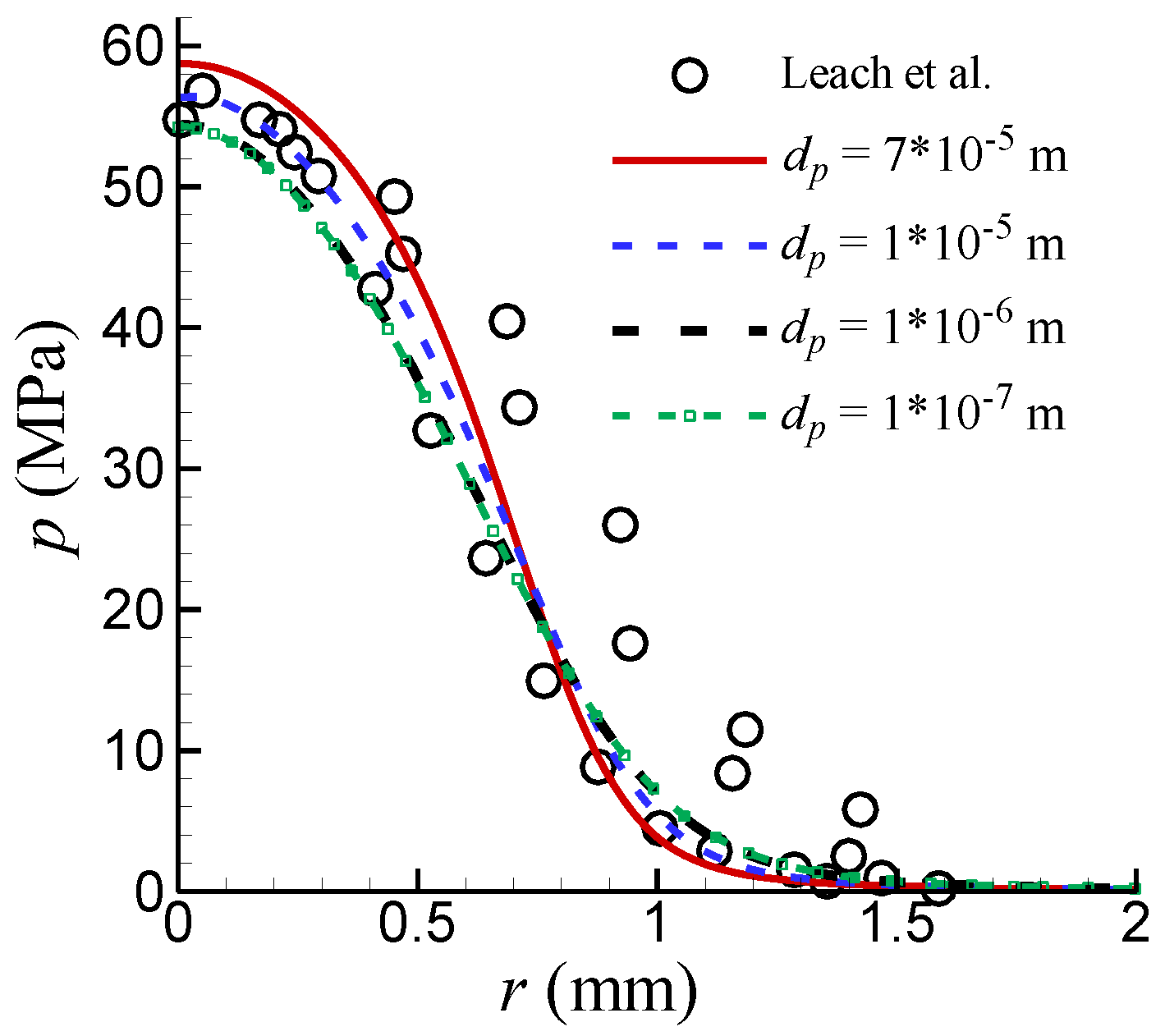
Figure 6.
Comparison of the effect of surface tension on the pressure distribution.
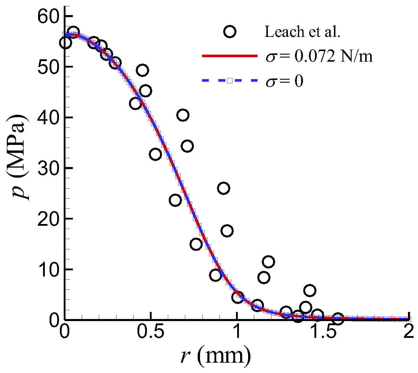

Table 1.
The physical properties of fluids.
| Fluid | Density (kg/m3) | Viscosity [kg/(m⸳s)] |
|---|---|---|
| water | 998 | 0.001 |
| air | 1.225 | 0.00001 |
Table 2.
The information of the reference case.
| Turbulence model | Turbulence treatment Method | Mean inlet velocity | Bubble diameter of secondary phase | Inlet condition |
|---|---|---|---|---|
| SST k–ω–φ–α | Mixture | 340 m/s | 1.0e-5 m | From a nozzle |
Disclaimer/Publisher’s Note: The statements, opinions and data contained in all publications are solely those of the individual author(s) and contributor(s) and not of MDPI and/or the editor(s). MDPI and/or the editor(s) disclaim responsibility for any injury to people or property resulting from any ideas, methods, instructions or products referred to in the content. |
© 2025 by the authors. Licensee MDPI, Basel, Switzerland. This article is an open access article distributed under the terms and conditions of the Creative Commons Attribution (CC BY) license (http://creativecommons.org/licenses/by/4.0/).
Copyright: This open access article is published under a Creative Commons CC BY 4.0 license, which permit the free download, distribution, and reuse, provided that the author and preprint are cited in any reuse.


