
Submitted:
10 February 2025
Posted:
11 February 2025
You are already at the latest version
Abstract
This work presents a toy universe grounded in classical logic, elementary natural arithmetic, and a touch of topology. The universe’s space is modeled as a finite, closed, discrete 3-torus with an additional non-spatial dimension of a carefully selected size. Each point within this space contains a fixed-size string of two-state elements, each possessing an ontological character. A few recurring patterns are observed across these layers: one based on the Euclidean distance from a central point, the second following a sinusoidal bit mask relative to the same point, the third is a unique ray marking a privileged direction, and the fourth is a spiral path. These patterns are dynamic, relocating after interactions, but keeping most data the same, displaced relative to the other layers. Time in this universe is discrete. Electric charge is represented by a single bit, weak charge by two bits, and color charge by three bits. The linear motion dynamics of the universe are dictated by a radial line of bits, while the rotational one, by an orthogonal spiral of bits. Gravity is interpreted as an extension of the static electromagnetic force, where a certain charge combination acts as a graviton, resulting in a super deterministic model reliant on a few input parameters. The unit of energy is the layer itself, which groups as particles, either localized or similar to photons, using a fundamental collapse mechanism. Particles leave behind a trace of their momentum onto the lattice. This allows for interactions with subsequent waves, leading to patterns that resemble quantum self-interference and opening a door for falsifiability of the model. This constructive approach establishes a universal cellular automaton framework. Foundationally, this work is in line with 't Hooft's cellular automaton interpretation of Quantum Mechanics.
Keywords:
cellular automaton
; non-locality
; emerging gravity
; unification
1. Introduction
Wheeler [1] coined the aphorism "it from bit." By this, he meant that anything physical—any it—derives its existence from discrete binary choices, or bits. This supports the notion that information has an ontological nature. The concept suggests that physics, particularly quantum physics, isn’t about reality itself but is rather our best description of observed phenomena. However, the nature of information remains elusive, especially regarding its physical or ontological aspects. In this study, the significance lies in conceptualizing the "bit," together with its update rules, as a two-state ontological entity.
In parallel, throughout his life, von Weizsäcker was primarily concerned with understanding the unity of physics. For decades, he and his collaborators pursued the idea of a quantum theory of binary alternatives (the so-called ur theory)—a unified quantum framework in which spinorial symmetry groups give rise to the structure of space and time. Aufbau der Physik [2] was primarily intended to provide an overview and update of this endeavor.
In this regard, cellular automata (CAs) are mathematical idealizations of physical systems in which space and time, an evolution parameter, are discrete. Their attractiveness comes from the notion that simple rules can lead to really complex behavior, tending to long and interesting evolutions.
An alternative representation of the universe is developed in this work using the cellular automaton paradigm. The theme has been explored for a long time (see [3,4,5,6,7,8,9,10,11,12] for example). However, these studies generally remain in the abstract realm or present very limited models. Here, a full 3+1 core specification is posited. Although it is a qualitative analysis for the time being, the model is amenable to immediate computational investigation. We are not asserting that the universe operates strictly as a cellular automaton (CA), but rather positing it as a convenient framework. Specifically, the representation of fundamental physical laws through a CA finite state machine facilitates computational inquiries. Kiefer, in [13], argues in favor of such a solution, stating that unless the spacetime structure is fundamentally discrete and the total number of degrees of freedom in the world is finite, the question of whether a given theory is the final one will remain undecidable, leaving an enduring ignorabimus.
Just classical logic and plain natural math, that is, bits manipulation, along with a hint of topology, are used in the dynamics, making up a constructive approach.
The greatest serendipity in modern physics is arguably the almost simultaneous discovery of the Schrödinger equation and the Born rule, which together provided the mathematical framework and probabilistic interpretation that revolutionized our understanding of the quantum world. While Schrödinger’s equation offered a deterministic description of wave-like behavior, it was Max Born’s insight that the wave function represents probabilities on ensembles that bridged theory with experimental reality. This unexpected combination not only shifted physics from a classical to a quantum worldview but also laid the foundation for countless technological advances and philosophical shifts about the nature of reality (see [14,15,16,17,18]).
The motivation behind this initiative stems from the challenge of reconciling Quantum Mechanics and General Relativity, the two fundamental pillars of physics, into a hypothetical theory of quantum gravity (see [19,20]). According to the author, this challenge arises from the presence of imaginary numbers in both Schrödinger’s equation and the spacetime metric, despite their usefulness as powerful tools. Unfortunately, these very tools have created an epistemological barrier that continues to exist today.
It follows, to be clear, that, at the foundational level, this work aligns with ’t Hooft’s cellular automaton interpretation of Quantum Mechanics. It is an attempt to identify what he calls the Ontological States (OS) [12], including their embedding in General Relativity.
Finally, the reader will be delighted when she/he sees that purely intuitive arguments are used, leaving out obscure concepts.
The paper is organized as follows: Section 2 begins with the foundational stage, defining the 3D space and time. Section 3 then introduces the bubble—the fundamental information-based element of the model. Section 4 and Section 5 define particles, along with a description of their initial formation state. The light frame and the Finite State Machine (FSM) are presented in Section 6. Section 7 illustrates bubble interactions and explores the role of charge conjugation, while Section 8 discusses the context of entropy. Section 9 provides key results. Concerns about undecidability are expressed in Section 10, while Section 12 succinctly contemplates the bridge between the model and the QM formalism, and Section 11 outlines potential future directions. Finally, Section 13 offers a summary and a synthetic interpretation of the model.
2. Space and Time
Let L be a huge natural odd number ( is the number of bits needed to represent this number). Space is represented as a cluster of cells arranged in a 3-torus topology, creating a finite, closed, and discrete structure. This configuration ensures that each edge of the space seamlessly wraps around to connect with the opposite edge, maintaining continuity across the system. Additionally, an extra, non-spatial dimension forms a layered structure consisting of layers (the extra 1 is to recover a required pair symmetry, since L is odd), with each layer containing cells.1
Time is treated as unidirectional and discrete, progressing in uniform steps. The extra dimension W can be visualized as extending through these layers, connecting them in a consistent, closed progression over time.
The seamless wrapping of trigonometric functions, such as the sine function, across the three dimensions of the torus enhances continuity, allowing smooth transitions and interactions among entities. This approach supports the potential emergence of charge quantization and other fundamental properties through the systematic evolution of the system.
Space is endowed with memory, recording the visits of the particles, a property that will be further explored in the next section and in Section 7.4.
2.1. The Cell Structure
Each cell contains the same amount of information characterized by a bit string formatted as shown in Table 1.
The input and output ports of each cell are conceptually linked through an FSM. This design choice emphasizes simplicity, as it operates using natural numbers and straightforward logical rules, steering clear of complex mathematical constructs. By prioritizing an ontological approach, we focus on the essential properties and relationships inherent to the system, rather than the computational power of a Turing machine [21] attached to each cell. This ensures a more intuitive understanding of the system’s behavior and maintains clarity in its foundational logic.
2.1.1. Physical Properties
The more intuitive variables are grouped here.
-
Charge ()Defined by bits q, , , , , . Charge encompasses various discrete properties associated with the particles, derived from specific bit values that define their interactions. They are the main responsible for the emergence of forces.
-
Pole (p)This bit designates a privileged direction, serving as a foundational entity closely associated with the emergent property of momentum.
-
Meta-pole ()This bit marks the path of a spiral orthogonal to the pole line. This spiral is the driver of spatial rotations and polarization.
-
Affinity (a)Groups bubbles into particles, facilitating the aggregation of smaller units into more complex entities. Affinity is essential for the formation of composite structures; without it, only a holistic universe would emerge. It is also responsible for the emergent phenomenon of entanglement and characterizes the track left by the particles in self-interference.
2.1.2. Wavefront Shaping
This set of variables and constants forms the mechanism for nearly perfect spherical wave propagation (with discrete constraints).
-
Euclidean distance (d)The Euclidean distance, d, is recorded in the cell during initialization to allow precise spherical propagation.
-
Sine mask (s)This bit represents a sine wave mask with a fixed two positive half-periods amplitude (number of points). It serves as the basis for wave-like behavior in the system. Electromagnetic collapse only happens when this bit is true.
-
Sine timing ()This natural number guides the evolution of the sine mask, functioning as an independent time variable for sine oscillations (arc).
-
Sine phase ()A bit indicating the sign of the sine wave.
-
Wavefront tick (t)A clocking mechanism based on the propagation of light, governing the timing of events related to the movement of wavefronts. It is a light step counter. This long natural provides a temporal reference for activities that depend on the spread of information or interactions.
2.1.3. Operational Variables
This model is intrinsically nonlocal, relying on mechanisms that extend beyond conventional spatial limitations. To support this nonlocality, it employs a very rapid timing system that ensures seamless coordination across the lattice. The variables defined below are essential components of this framework, managing the dynamics of relocation, internal processes, and wavefront propagation.
-
Relocation offset ()This natural vector determines the reissue address, guiding the position where an element is reallocated within the system. This variable controls the adjustment needed to realign or reposition bubbles in the lattice. The displacements follow the general rulewhere:For an odd L, the coordinate of the central point is:
-
Housekeeping tick (k)This long natural2 is an atemporal clocking mechanism, used for maintaining internal processes. It operates in coordination with the main temporal evolution, ensuring the system’s consistency and managing important tasks.
-
Collapse flag ()A bit indicating the occurrence of collapse in the interaction. It is used the warn the components of a particle that a collapse occurred (see Section 6).
-
Frequency (f)This counter reflects the number of superposed bubbles with a common affinity.
2.2. The Host Lattice
The space described above is occupied by three coexisting 3D-Euclidean spatial lattices made of cells each, repeated in W layers (that is, cells total), serves as an absolute inertial reference frame. All cells within each layer pulsate in unison, incrementing alternately a couple of evolution counters (k and t) and exchanging information with their seven neighbors (six in dimensions x, y, and z , and one in dimension W, which facilitates the transfer of information between lattices and detects interactions). This exchange occurs alternately, ensuring time homogeneity is recovered every two clock ticks, grouped in four passes (see further details below), thus configuring a cellular automaton.
The distance between cells along the three spatial axes corresponds to the fundamental quantity X in the real world. The arithmetic employs L as a modulus in most calculations.
The three lattices mentioned above are referred to as main, draft, and mirror. The main lattice is the current lattice used in interactions; draft is the modified data; and mirror is used in comparisons of bubbles in different W addresses, being modifiable too. A cell is capable of modifying its own draft and mirror cells, but not itself.
3. Fundamental Patterns
3.1. Definition of Bubble
A bubble is an expanding spherical wavefront of information organized across cells within a common layer. Spherical propagation is determined by comparing the Euclidean distance d, precomputed and stored in each cell, to the evolution parameter t.
3.2. Relocation and Orphans
Bubbles are re-emitted either immediately after an interaction or through wrapping. When the bubble is reissued, the previous wavefront continues to propagate until it fades through wrapping. In this state, the bubble is referred to as an orphan, meaning it has affinity disabled, but is still capable of non-collapsing interactions. In this case, for the outer cells, set during the relocation step (see Section 6.5). The orphan does not interact with photons, because , but interacts with gravitons (see definition in Section 4.3). Neutral orphan pairs do not interact electromagnetically.
A bubble can only be relocated to a point on its active surface. This guarantees that the speed of light will never be violated. Since wavefront propagation is guided by Euclidean distance information pre-assigned to each cell, when a bubble is re-emitted due to interaction with other bubbles, all pertinent cell information must be shifted to the new position determined by the variable . This ensures that the bubbles are relatively displaced with respect to each other. The final operation sets at the center cell of the relocated pattern. Relocation is the main consequence of an interaction.
3.3. Charges and Motion Patterns
Charges, or more precisely, fundamental charge fragments, are constant-valued bits that govern the interactions among bubbles. Their properties draw inspiration from the Standard Model of particle physics.
The electric charge q is associated as ever with attraction/repulsion, while the weak charge with its two bits and , or chirality, is associated with congruence. Since the universe is closed, the addition of an extra bit guarantees this sense of congruence. The sector with , will be called Orbis,while the sector with will be called Umbra. On the other hand, the three color charges , , enforce the strong force structure. Color codes are , , , , , , , for neutral, red, green, antiblue, blue, antigreen, antired and anti-neutral, respectively. Let signature be . A bubble is matter M if , or antimatter , otherwise. Also, it is neutral N, if or anti-neutral , if . The definition will be used in the practical implementation [22].
The two path patterns formed by bits p and , or pole and meta-pole, defined during initialization, complement the interaction quantities. One is a linear distribution, while the other is a spiral path.
3.4. Sine Amplitude
Each layer contains an embedded sine amplitude, represented by a spherical mask formed by the s bits, within its cell structure (see Section 2.1). This is a uniform spherical distribution of points modulated by the sine function from 0 to radians, that is, a full period. For superimposing bubbles, the sine amplitude is independent of the primary timing variable t, using instead, which relates to photons and other bosons whose frequencies are multiples of the fundamental cycle (see Figure 1).
The sign of this amplitude, the bit, which flips at the end of each half-cycle of the sine pattern, governs the appropriate behavior, essentially electromagnetic interference and resonances, enforcing the harmonic character of the natural law.
3.5. The Speed of Light and the Size of the Universe
We can now state the following constraint on the fundamental quantities:
where c is the speed of light and is the number of ticks per frame. Estimates for the values of X and L(truncated to a natural) are taken from Appendix A
and
where is the Planck length. From this, we calculated the size of the universe as (the Grand Cube diagonal).
4. Particles
Bubbles form the composite structure of particles, which can be studied through experimental physics. A particle is characterized not only by the proximity of its bubbles but mainly by the fact that most of these bubbles share the same affinity value a.
Two superposing bubbles can form a pair if they share a common affinity value, (see rule in Section 6.2.1). When two bubbles form a pair, the action of their weak or strong charges (but not the electric charge) is inhibited if they are complementary. Both bubbles are reissued in an interaction involving a pair. In general, the combinations formed correspond to boson fragments. A bubble that does not form a pair is called a singleton.
4.1. Fermions
A particle is classified as a fermion when its structure contains more than just paired kinematic components. Fermions typically exhibit a balanced average of bubbles with identical charges (the up quark is a specialized pair treated below), sustained through dynamic charge quantization (see Section 11.1). Additionally, fermions often include pairs that act as propellers, facilitating movement. Overall, fermions form a small, undetectable volume, "punctiform" cloud of bubbles, surrounded by concentric orphans created through frequent re-emissions, thus establishing their field.
Quark confinement originates from the prioritization given to color cohesion and quark-gluon interaction over other forces. In contrast, within an atom, electrons naturally distribute around the nucleus according to spherical harmonic distributions.
4.2. Bosons
A particle is classified as a boson if all its component bubbles form superposed pairs. Specific types of pairs that fulfill this criterion include a photon fragment and other gauge-boson fragments. Each of these roles involves a pair structure where some or all charge bits differ except for the bit, that is, they are sectorial particles.
The defining characteristic of a photon is that all its pairs are superposed at the same point. In contrast, for other bosons, such as the and Z bosons, in which the pairs form a "punctiform" cloud of multiple islands of superposing pairs, somewhat similar to the behavior observed in fermions.3
4.3. Specialized Pairs
The golden rule for specialized pairs is that, unlike bosons, they do not form multi-pairs, giving them a fermionic character.
Neutrino and antineutrino pairs, and , possess color values and , respectively. Inter-sector neutrino fragments are unique in that they do not interact via the weak force, rendering them sterile in this sense. The small mass of neutrinos is the sum of their two components and additional contributions from propellers (relativistic mass).
The up quark fragments u exhibit equal, nontrivial colors and a positive charge in the case of Orbis.
A distinct kinematic role of a pair is that of a propeller, which continuously repositions other bubbles, forming the fundamental mechanism for inertia and motion. The propeller adds to the relativistic mass of the propelled fermion.
Finally, pairs that exhibit all complementary charge characteristics are termed gravitons. These pairs can operate in both Orbis and Umbra.4. Each graviton pair has a fixed, absolute, oscillation frequency of 2, corresponding to their fundamental resonance in this dual framework. Gravitons contribute to the static interactions in both sectors. Without the graviton, matter from Umbra would appear entirely inert, and gravity would not exist. The mechanism by which gravitons contribute to gravitational interactions is further elaborated in Section 11.2.
5. Initial State
5.1. Overview
Let S be the total number of states resulting from the combination of all cell values, all positions in the lattice and all bubbles. Assume there is an endless period loop with definite net Shannon-like entropy [23] that corresponds to the real world. This very, very long cycle, technically a Poincaré cycle, must ideally include the initial state, ensuring no loss of information (see Section 8). Among the countless possibilities, we choose the following platonic solution for the initial state problem described below.
The initial state sets up the configuration of all cells within the lattice. At , when all bubbles are superposed at the center (, , L/2), this state is referred to as the singularity.
Additionally, the same initialization procedures are mirrored on the draft lattice, ensuring consistency and coherence across both structures.
Although high-level functions and real numbers are used in defining initial states, this does not violate the foundational approach of using natural numbers exclusively in the dynamic process. The real-number values and functions serve only as intermediaries for calculation, while the resulting natural number values are assumed to be imprinted directly onto the space structure by fiat. This approach preserves the integrity of a natural-number-based dynamics, grounding the system’s evolution firmly within the discrete structure of the lattice.
5.2. Miscellaneous Procedures
First, the vector is initialized with the appropriate Cartesian positive coordinates (). These values remain constant but accompany the bubble during relocation. Additionally, the time counters t and k are initialized to zero. The vector is set to zero.
The weak charge is defined as and , while the electric charge is given by . The color is determined as . Finally, all bubbles are initialized as . These choices result in a very regular pattern of charge distribution.
This and the following pattern creation is then replicated across all layers in dimension W.
5.3. Computing the Euclidean Distance
The Euclidean distance is a function of the spatial coordinates given by
This justifies, once again, the need to adopt an odd value for L: a central point is necessary for this pattern to be properly defined.
Algorithm A1 in Appendix B shows how to apply this formula.
5.4. Computing the Sine Cloud
The same applies to the root sinusoidal mask, which is given by Algorithm A2 in Appendix B. Note that this gives a full cycle with positive values. In a 3-torus, the sine function will wrap around seamlessly in all three dimensions, ensuring that there are no discontinuities. This property allows for a continuous representation of various physical phenomena across the toroidal structure. Each dimension can be thought of as a periodic loop, where values of the sine function are confined within a range that recurs indefinitely.
It is shown in Figure 2 two shells with points distributed following the sine pattern.
5.5. Computing the Auxiliary Reference Bases
The pole is a bit used to enforce linear motion, while the meta-pole bit is used to enforce spatial rotation. To generate the pole and meta-pole points, it is necessary to calculate an auxiliary set of three orthogonal vectors , or base. The first base vector is tied to the poles’ initialization, the second has to do with the meta-poles, while the third will be used to define a plane to be used to build a 3D spiral that defines the meta-pole bits themselves. Note that the bases are temporary data used to initialize the pole and meta-pole bits, which, yes, are part of the automaton. Each basis will be used to initialize one layer in the W dimension.
To ensure a consistent and uniform initialization of the pole direction, each cell’s pole base vector must be configured to span steradians on the last shell (radius ), guided by Algorithm A3 in Appendix B. On the other hand, the generation of vectors for each cell aims to ensure that they are orthogonal to the direction. This ensures that the momentum aligns with the rotational dynamics without interfering with the rotational direction defined by .
If the is not aligned along a principal axis (e.g., not parallel to the x-axis, y-axis, or z-axis), the vector can be chosen using a simple cross product with a fixed axis to ensure orthogonality. For example, is not along the z-axis, set the momentum vector as: . If the base vector is along the z-axis, the x-axis can be used instead to define the meta-pole: as: . After computing the orthogonal vector, the two vectors are normalized and then used to calculate , completing the orthogonal basis.
5.6. Building the Canonical Spiral
The canonical spiral is defined in the canonical reference frame . It is a modified Archimedean spiral whose z coordinate increases as the angle increases. The following equations are used to calculate its points:
The canonical spiral (see Figure 3) is then copied to each base defined above using a rotation matrix , which transforms points from the canonical frame to the new reference frame. It is constructed using the rows , , and :
To rotate a point in the canonical frame to the new reference frame, compute:
5.7. Activating the Pole and Meta-Pole Bits
Vector is then used to mark the pole bits p from the center to the target point, following the well-known Bresenham 3D line algorithm. The points forming the spiral identify the cells that must have their meta-pole bit activated.
These spiral patterns, parametrized across all layers, induce the emergence of light polarization.
6. The Light Frame
Conceptually, this universal cellular automaton works based on instances of a Finite State Machine connecting the bits of neighboring cells. The light frame is divided into four steps: convolution, diffusion, relocation, and transport.
6.1. Definitions
To give support from now on, let us define the following natural constants related to the light frame and interactions:
-
DIAGDefined as , this constant measures the diagonal length of the 3D lattice. It is useful for determining maximum interaction distances within the lattice.
-
RMAXDefined as , it represents half the diagonal length of the lattice, setting a maximum radius a bubble can achieve before wrapping itself.
-
FMAXSet to , this constant represents the maximum number of superimposed bubbles that can coexist in the lattice. It ensures that the amplitude of the sine wave mask remains meaningful by limiting the interaction between overlapping bubbles. This is crucial for maintaining the integrity of the wave propagation and preventing distortions caused by excessive overlapping. It is used for consistency check only, and is supported by the Sampling Theorem [24].
-
CONVOLUTIONRepresents the convolution window, defined as W. This constant determines the range in which the initial convolution process is performed during the light cycle.
-
DIFFUSIONDefined as , this constant specifies the maximum diffusion range along the W dimension during a collapse event. It acts as a preparatory step for relocation if any collapse bit is true at the start, then by the end, all layers are aware of an imminent collapse.
-
RELOCATIONThis constant, defined adding ticks to the diffusion step, specifies the region dedicated to bubble relocation after initial interactions and diffusion have taken place. It ensures that any necessary adjustments to the positions of particles are made.
-
TRANSPORTThis constant, defined by adding ticks to the relocation step, complement the relocation process in the event of parallel transport.
- FRAME This constant holds the same value as , but its semantics differ. It represents the total duration of the light step, encompassing all phases: convolution, diffusion, transport, and relocation.
6.2. Interaction principles
Before considering the light frame itself, let us discuss a few guiding principles adopted.
6.2.1. Aggregation and Dissolution
As bubbles interact, they may aggregate by sharing a common affinity, thereby forming particles. The general rule is: the smallest affinity value prevails. For instance:
When particles dissolve, they assume their layer indices:
If the interaction is between a singleton and a pair, then the pair takes the affinity of the singleton.
6.2.2. Charge Conjugation
Charge conjugation is a principle that governs interactions between bubbles in the CA. Charges impose specific constraints on one another, ensuring that interactions occur in well-defined ways, ultimately aiming for neutrality.
Neutrality can be defined either for an isolated bubble or for a pair of bubbles. For electric charge, represented by a single bit, neutrality can only be established for a pair of bubbles with opposite charges, resulting in net neutrality. Since an isolated bubble contains only one electric bit, neutrality cannot be defined in such a case.
For weak charge, represented by two bits, neutrality arises from how the pair of weak bits combine to determine handedness in both the Orbis and Umbra sectors.
In the case of the strong force, which utilizes three bits, inner neutrality corresponds to the state 000, while inner anti-neutrality corresponds to 111. A pair of bubbles with complementary color bits (e.g., 101 and 010) also exhibits net neutrality.
The general rule for interactions is then that the resulting combination of charges must achieve a neutral state.
6.2.3. Static Interaction
The static interaction, namely the Coulomb and magnetic forces, happens through the direct alignment with a graviton. When the graviton interacts with an electron, it is reissued at that point. That is, the graviton is a central piece in a static interaction. Gravitons are reissued along the way of a singleton, active or orphan, increasing the probability of interacting with an electron in that region, becoming one of its propellers (see Section 7.2.1 for more details).
6.2.4. Pair x Singleton Interaction
An interaction filtered by the conditions pole x pole or meta-pole x meta-pole, and sine x sine provokes collapse. In the other cases, the interaction is triggered by the singleton’s pole.
6.3. Convolution
Convolution is the first step in the light frame. It contains the main interaction rules. During this phase, the mirrored image of the main lattice generated in the swapping phase is used as follows. Each site is compared to its neighbor in dimension W, in a circular fashion. One important condition is that the cells must be active wavefront cells (). Algorithm A4 in Appendix B shows the main logic adopted. Also during this step, as the pairs are being identified and stacked, the angle that selects the sine point density is incremented accordingly (frequency).
In the convolution step, the formation (or reformation) of particles occurs.
The comparisons are divided into two main groups: the bubbles are superimposing, or the bubbles have distinct origins.
6.3.1. Superposing Bubbles
Two overlapping bubbles can form a pair if they satisfy the following conditions:
- They both have frequency equal to one, .
- Their combination is not forbidden by these rules:
The formation of multi-pairs is made during this step too. Pairs are allowed to superpose if they satisfy these rules:
Net charge calculation and affinity fusion, implicit in the formulas, are done as necessary, seamlessly.
6.3.2. Distinct Bubbles
A number of potential interactions may occur when the bubbles are distinct. The algorithm referred to above shows schematically how it happens for most cases.
If two singletons have opposite charges, we have annihilation, with both bubbles being re-emitted from the contact point and their affinity receives its default value.
If the two singletons share the same affinity, but have different charges, then the singleton whose pole is the contact point is reissued from the contact point. The other bubble is reissued from the parallel-transported pole.
If the charges of two singletons are equal and the pole of the first bubble hits any point of the active surface of the second bubble, then we have fermionic cohesion. The bubbles receive the same affinity; the first bubble is re-emitted from the contact point, while the second from its meta-pole.
6.4. Diffusion
This phase propagates states across the W dimension if necessary. A non-trivial relocation offset is used to reposition the bubble in the 3D space, and the bit is utilized during the traversal of all layers in the W dimension. If any bit is true at the start, then by the end, all collapse bits will be true for all bubbles sharing a common affinity. The spread of the collapse bit in the W dimension is necessary for identifying all fragments that compose a collapsing particle.
6.5. Relocation
The final part of the light step addresses bubble relocation itself. Bubbles shift in specific directions (north, west, down) until they have completed their relocation process. During this phase, the parallel transport mechanism of inertia is finalized, ensuring the bubbles undergo their last relocation.
When the relocation is complete, bubble variables are prepared for the next cycle. If the time frame completes, the k counter resets to zero, preparing the system for the next iteration. At the conclusion of the process, all vectors will have a null value.
6.6. Main Lattice Updating
After each tick of the k clock, the modified data in draft must be transferred at once to the main lattice. First, if the k counter is within the window, the draft lattices are shifted in the W dimension to disalign them from the current draft lattices to convolute.
The current lattices then receive the content of their draft lattices. Also, at the beginning of the evolution step, the mirror lattices are massively updated with the current lattices’ content, thereby preparing the system for comparisons in the W dimension (Section 6.3).
7. Interaction Details
Some aspects of the interactions detected during the convolution step will now be elucidated.
7.1. Parallel Transport
Inertia is acquired by a parallel transport mechanism. It happens between two bubbles with the same affinity and trivial vectors when the pole of one bubble hits the surface of the other bubble. First, the bubbles have , then .
Both fragments relocate to their own pole until , and then the bubble 2 relocates by to the parallel transported position.
The propeller naturally emerges as a pair in order to avoid static interaction; this formation is not externally enforced but results from intrinsic system dynamics. It represents a fragment of a photon, where the pair exhibits symmetric charges. This symmetry effectively bypasses the priority of interactions mediated by forces such as the Coulomb force.
Furthermore, when a multi-pair photon interacts in this manner—acting as a propeller—a specific pair detaches from the photon to become a distinct propeller. This detachment facilitates subsequent processes, including inertia and relocation within the lattice framework.
7.2. Charge Combination
The weak charge bit separates the interactions into two groups: same-sector and inter-sector. We will first describe the same-sector () cases and later the inter-sector case in what follows.
7.2.1. Coulomb Interaction
Coulomb attraction and repulsion occur in two steps: a) the p bit of an orphan of the first electron hits an active cell of a graviton. If they are aligned or antialigned (checking their x vectors), the graviton is reissued from the contact point, carrying the affinity of the orphan, in this case W; b) then, the p bit of the second electron, which was aligned with the graviton, hits an active cell of the graviton being reissued, carrying the affinity of the singleton, that is, it becomes a propeller with the correct direction.
7.2.2. Magnetic Interaction
The magnetic case involves the meta-pole instead of the pole p. These interactions are valid for interactions between electrons, quarks, and W bosons.
The emphasis of propellers on the pole rather than the meta-pole significantly influences the resulting propeller: the faster the particle moves, the more likely it is to be perpendicular to its direction of motion.
7.2.3. Neutrino Interactions
Let be a pair of complementary electrical bits. A neutrino fragment is a pair of bubbles with charge content , while an antineutrino fragment is a pair with both bubbles having charge . (Anti)neutrino fragments interact with (right)left-handed particles only.
This final rule applies to all weak sectorial interactions, determining the disintegration nature of this force.
7.2.4. The Up Quark and Down Quark Fragments
We can behold possible combinations of color properties between pairs of bubbles in the table of Fig. Figure 4. (Anti)quark fragments have non-trivial color and are marked as q or , (anti)neutrinos are and , gluons are g, and photons are . Since half the gluon fragments are right-handed, they are shown as photons. The cells marked as blue, if having both quarks with electrical charge , may form an up quark fragment.
An up quark (u) can be any of the +R+R, +G+G or +B+B fragment pairs, while a down quark (d) can be any of the -R, -G or -Bsingle fragments. When we combine three of these quark fragments into a proton fragment uud, we get an uncompensated color. The matter end of the gluon may fit this lack, but in return it generates an antimatter end, and so on, in a dynamic balance. Naturally, it follows that the electron fragment must be -N,-N,-N.5 An important remark fits here: the quantity of up quark fragments in each sector is crucial in defining an upper limit for the production of protons and, consequently, atoms.
7.2.5. Symmetry Breaking after Singularity
At the singularity (initial state), all bubbles overlap, necessitating an additional interaction rule to achieve separation. The adopted rule is as follows:
During the convolution step, if a spatial address contains two overlapping bubbles with fully symmetric charges, the bubbles are re-emitted from their respective poles. This process rapidly disperses the singularity, facilitating the separation of Orbis from Umbra. Let us call this segregation.
7.2.6. Singularization
The counterpart to segregation is singularization. In the distinct case, partners with fully complementary charges are re-emitted from a single pole. This mechanism helps to enforce the emergence of a Poincaré cycle by adding a temporal symmetry to the model.
7.3. Collapse
The destruction of a particle due to annihilation or light-matter interaction is performed during the light step, but only in the annihilation case, the affinity properties will be redefined to their default values.
where w represents the index of the W dimension. Bubbles are now raw material for the formation (or recreation) of new particles in this case.
7.4. Self-Interference
As mentioned earlier, space has a memory that records the paths taken by the particles, contributing to the phenomenon of self-interference, similar to what occurs in the double-slit experiment [25]. The approach used here was initially proposed by Sciarretta in [11], utilizing punctiform stochastic particles.
The core idea is to leave a trace of the particle’s lifetime in the lattice as their fragments, or bubbles, move through space, propelled by inertia agents, the propellers. This trace is materialized by the last affinity value a and the last sine phase left in the lattice.
During the convolution step, the properties of new and old bubbles are compared. If a normal cohesion results. Rather, if , only the new bubble is reissued. This disturbs the dynamics of the fermion, resulting in detectable interference patterns.
Notice that this mechanism works just for singletons, or fermion fragments, not for pairs.
8. Entropy Considerations
8.1. Shannon-Like Entropy
Shannon entropy provides a measure of the randomness or disorder in a system. For a 3D cellular automaton, it quantifies the uncertainty associated with the system’s states. The formula for Shannon entropy, as introduced by Shannon [23], is:
where H represents the entropy, is the probability of observing a particular state i, and denotes the base-2 logarithm.
8.2. Defining the State Function
In practice, calculating entropy based on the exact configuration of the entire system is impractical due to the negligible probability of repeated configurations. To address this, we define a state function that selects specific properties of interest to represent the state of a cell. These properties include:
- Spatial Position: The coordinates of the cell within the lattice.
- Charge: A physical property of the cell.
These variables are combined into a single numerical value representing the cell’s state. Each unique combination of these variables corresponds to a distinct cell state.
For simplicity, the entropy computation considers only the central cell in each layer (W) of the 3D lattice. If the cell does not belong to a pole, its state defaults to zero.
The total number of possible states is calculated as:
where L represents the lattice size along each dimension.
8.3. Defining the Era
Entropy is computed over a defined era, which represents a segment of the system’s evolution. Assume a Poincaré cycle estimated as P light steps () is known, and the entropy graph consists of bars. The era is defined as:
8.4. Calculating Entropy
Entropy is calculated using Equation (9) following these steps:
- Collect State Occurrences: Save the state of the central cell in each W-layer at the end of every light step ().
- Count State Frequencies: Record how often each state appears within the lattice over the duration of an era.
- Determine Probabilities: Divide the count of each state by the total number of states (N) to compute its probability .
- Compute Entropy: Apply Shannon’s formula (Eqn. 9) to compute the entropy H.
The resulting entropy values provide insights into the complexity and evolution of the automaton, uncovering patterns and emergent behaviors. Specifically, they help identify the presence of a Poincaré cycle and determine whether information loss prevents the system from returning to its initial state.
9. Results
To illustrate the concepts discussed thus far, we have developed a few practical examples.
9.1. A charge Conjugation Study
A small program (see Ref. [22], file combine.c) was created to check the combination of charges. A total of fragments, with their charges evenly distributed, were randomly combined in several million attempts and the averages tabulated. It was assumed that only ’hydrogen atoms’ are formed.
Since the strong force dominates, a probability value of 0.001 was assigned to the search for up quarks and 0.999 to gluons. These values were calculated based on the smallest possible set of charges. The search was conducted in four stages. First, gluons and up quark fragments were targeted (fragments of electrons were also included, as their existence depends on the number of generated up quarks). Next, photons and neutrinos were sought, followed by fragments of the W and Z bosons, and finally, anti-atoms were examined.
The results can be seen in Table 2. The leftover, that is, the bubbles that could not form a pair or a singleton, reveals a highly ionized environment, that will be attenuated by inter-sector interactions, resulting in an increase in the photon count. These data resemble roughly a few simple ’atoms’, while the photon fragments could form a few multiple pair photons. One can then speculate that the unmatched quark fragments could form mesons or virtual quarks or even contribute to dark matter (50% + 25%), and that the Umbra contains more antimatter than Orbis. All in all, it makes sense as a toy universe.
Unfortunately, one key figure for model validation, represented by the proton-electron mass ratio, appears in this simple analysis with a value of just 1187 for both sectors, rather than the empirical value of (CODATA [26]).
9.2. Computing the Poincaré Cycle
A highly simplified simulated implementation of the FSM CA is being developed (see Ref. [22]). Although dimensionally small, it will eventually be fully operational, incorporating all the rules. This model will enable the calculation and visualization of its Poincaré cycle in a straightforward manner.
At first glance, in a closed system like this, entropy is expected to initially increase, followed by a phase of consistent decrease, marking the completion of a full Poincaré cycle. Using the definitions provided in Section 8, an entropy plot for the model can be generated.
The following section discusses potential challenges and limitations of this approach.
10. Undecidability and Long-Term Dynamics
A critical challenge in our model is understanding its long-term dynamics, particularly the determination of a Poincaré cycle. However, the computational complexity underlying its dynamics introduces significant undecidability concerns, especially when scaling the model to larger sizes. Due to its richness, this CA can be computationally equivalent to a Turing machine [27]. This equivalence means that certain questions about its evolution, such as predicting whether the system will eventually return to an initial state (a Poincaré cycle) or stabilize, are undecidable [28]. Specifically, determining if the given initial configuration will lead to periodicity or chaotic evolution cannot be resolved algorithmically. Moreover, increasing the grid size by scaling L (the linear dimension of the CA grid) exponentially enlarges the configuration space, significantly compounding the complexity of detecting periodic or other predictable behaviors [29].
In the broader context of cellular automata, the interplay between undecidability and long-term periodic behavior becomes even more intricate when considering multiple interacting systems, such as parallel CA grids or random walks (an ergodic process). For instance, in the case of n independent random walkers on a three-dimensional toroidal lattice of size L, the expected time for all walkers to simultaneously return to their initial positions scales approximately as
where the probability of a single walker returning to its starting point is approximately 34%, as shown by Watson [30]. This result underscores the scaling effects introduced by increasing the number of interacting entities, revealing how larger systems can give rise to emergent behaviors that are both complex and unpredictable [31].
The Pigeonhole Principle guarantees that the system will eventually revisit a previous state, as the number of possible configurations is finite [32]. This re-visitation implies that the CA must either stabilize (reach a fixed point) or enter a periodic cycle (a Poincaré cycle). However, the time required to detect periodicity can be exceedingly long, potentially growing exponentially with the grid size L. Although the limited scale of the implementation identified a Poincaré cycle, the undecidability of CA dynamics means that no general method can predict the cycle’s length or guarantee that it even exists [7].
10.1. Scaling and Emergent Dynamics
Going in the opposite direction, since this CA relies exclusively on local interactions, the periodicity observed in smaller grids is determined by localized patterns and their propagation rules. When scaling the grid from size L to (where k is a positive integer), these localized dynamics remain fundamentally unchanged. However, the larger grid introduces more potential for diverse local interactions, which can complicate the emergence of periodicity at the global level. If the periodicity observed in smaller grids results from stable, self-contained patterns, these patterns may replicate predictably in larger grids, leading to scalable periodicity. Conversely, the increased number of localized interactions in larger grids can result in new emergent structures that disrupt or modify periodic cycles.
Periodic boundary conditions enable patterns to propagate seamlessly across the grid edges, maintaining continuity in localized dynamics. However, the expanded grid size increases the likelihood of interactions between multiple localized structures, potentially altering overall dynamics. Scaling may also lead to longer periodic cycles as localized patterns traverse the larger grid. These extended cycles, while predictable locally, may exhibit more complex behavior over time.
The initial segregation Orbis x Umbra also contributes to a longer Poincaré cycle.
11. Conjectures and Prospects
This work represents the tip of the iceberg. The challenge now is to delve into the many conjectures that emerge from it, prove them, perhaps with minor adjustments.
Just a few examples are considered here.
11.1. Charge Quantization
A subtle "defect" in the CA model arises during its initialization (see Section 5). Attempting to define the pole lines as an isotropic distribution within the lattice’s discrete and "squared" constraints introduces asymmetries. This defect facilitates the emergence of quantization, analogous to charge quantization in physical systems. The discrepancy between the chosen dimension for the W dimension () and the number of isotropic directions creates a defect that acts as a useful artifact, enabling charge quantization. This quantization organizes the system into discrete states, reducing chaotic evolution and promoting periodic behavior. On smaller grids, it manifests as localized, stable patterns. When the grid size scales, these quantized states remain robust, supporting scalable periodicity and recurring cycles in larger grids.
A key mathematical underpinning of this quantization is the concept of the winding number. The winding number measures the total number of times a vector field winds around a point or axis, serving as a topological invariant. In the CA model, the defect-induced asymmetries can be associated with a nonzero winding number, which enforces the discreteness of the system’s state space.
To achieve charge quantization, and consequently the quantization of other fundamental properties, it is essential to introduce a mechanism that mimics the effect of a magnetic monopole. In the context of our discrete 3-torus model, this can be accomplished by ensuring that the property vector s exhibits non-trivial winding around at least one of the non-contractible loops of the torus. This behavior is analogous to the presence of a magnetic monopole, which, in conventional theories, enforces the quantization of electric charge [33].
11.2. Emergence of Gravity
The model posits that gravity arises as a residual effect of electromagnetic interactions, emerging naturally within the cellular automaton framework through the interplay of photons and gravitons. Acting as super photons, gravitons possess properties that allow them to mediate interactions across the two overlapping sectors of the toy universe, Orbis and Umbra. While ordinary photons are restricted to sector-specific interactions, gravitons provide a mechanism for fundamental connectivity in a universe otherwise marked by a strong separation between these domains. Through this dual-sector capability, gravitons redistribute energy and charge, contributing to phenomena analogous to dark matter.
However, their direct influence on distant masses diminishes due to the cancellation of antagonistic forces induced by their interactions. What remains is a residual, geometry-driven attractive force that underpins the emergent gravitational effect.
An additional factor in this framework is the gradual energy dissipation observed as photons travel great distances. This aging process, intrinsic to the cellular automaton, parallels photon redshift in its effect. As it propagates, an energetic photon suffers small interactions with errant singletons and electrons, without collapsing. Over time, this energy dissipation subtly shifts the light spectrum to a redder region.
11.3. Stochastic Behavior
The richness of the regular patterns that intersect to determine an interaction, combined with the large number of bubbles that form the particles, results in seemingly random outcomes, despite the deeply deterministic nature of the model.
11.4. The Hofer Effect
A particular challenge is to verify the Hofer effect, the expected tendency for all spins of a localized particle to align radially either inward or outward (spin up/down), as predicted in Hofer [34]. In that work, there is an explanation of how magnetic effects emerge from symmetry breaking of this spherical pattern, thereby supporting the Stern-Gerlach experiment.
11.5. Particle Zoo Panorama
As mentioned, this is a toy model still under construction, with aspirations to evolve into a full-fledged theory. It serves as a framework to speculate on the composition of known particles in light of the proposed model. In the discussion that follows, the fragments will be characterized by their charge content: . For example, we designate the fragment 100000 as and 001111 as , and so forth.
11.5.1. The Electron Neutrino
The electron neutrino is formed by a single [] pair and additional propellers. Yet the anti-electron neutrino uses the pair [].
11.5.2. The Electron
The electron is formed by a quantized number of fragments, a great number of electron neutrinos and a variable number of propellers. The positron, or anti-electron, uses fragments instead. These are for Orbis, in the case of Umbra, all bits are inverted.
11.5.3. The Muon Neutrino
The muon neutrino is formed as plus additional propellers. It is like an electron neutrino, but with a compensated antimatter part.
11.5.4. The muon
The muon Consists of a quantized number of fragments, a large number of muon neutrinos , and a variable number of propellers. The classical study conducted by Itô in [35] suggests that this configuration stabilizes at the second harmonic of the electron’s radial vibrational state.
11.5.5. The Tau Neutrino
The tau neutrino is formed as plus additional propellers. It is also like an electron neutrino, but with a compensated antimatter-enriched part.
11.5.6. The Tau
The tau is formed by a quantized number of fragments, a great number of tau neutrinos , and a variable number of propellers.
11.5.7. Leptons Decay
In the Standard Model (SM), the decay products typically include one neutrino or antineutrino. However, in our model, the large number of neutrinos are entangled, sharing a common affinity. When one neutrino interacts via the weak force, all other entangled neutrinos collapse to the same point. This phenomenon gives the appearance of a single, energetic neutrino, as the observable outcome remains indistinguishable, in agreement with the SM predictions.
11.6. Compound Particles Half-Lives
Protons, electrons, and electron neutrinos are composed exclusively of bubbles, without their corresponding anti-bubbles. This unique composition is a key factor in their exceptionally long half-lives, potentially making them stable. In contrast, particles containing both bubbles and anti-bubbles are significantly less stable. Their shorter half-lives result from the likelihood of annihilation events between bubbles and anti-bubbles within their structure, leading to their transient nature.
The neutron embeds lots of electron antineutrinos, which bind the negative charge to its inner proton. This explains the decay of the free neutron.
11.7. Heavier Quarks
The framework suggests that the other quarks follow the composition of leptons, with additional neutrinos and antineutrinos, besides a variable number of propellers.
11.8. The Abundance of Neutrinos
Despite the relatively small number of neutrinos observed in Table Figure 4, their large cosmic abundance can be understood in light of their extremely low mass, approximately five million times smaller than the mass of an electron. This characteristic allows neutrinos to exist in enormous quantities across the universe, even if their presence appears limited.
12. The Bridge
Of course, the ontological states () representing each configuration of the CA cells cannot form superpositions. But, an orthonormal set of ontological states can be used as a basis for a Hilbert space. Given a subsystem of the universal automaton, the general recipe is as follows: find a permutation operator as a matrix containing a single 1 in any row or column. Diagonalize it, obtaining the eigenvalues and eigenvector matrices. Identify a Hamiltonian matrix as the exponent in . Use the eigenvalue matrix to bring this Hamiltonian back to the ontological basis. Form linear combinations of the ontological states |A〉.
where is a quantum state or "template" and is a complex coefficient.
Now we are able to use the operator mechanics machinery, in particular the Schrödinger equation, to analyze it:
13. Discussion
13.1. Origins of the Model
A simplified model universe was constructed from fundamental principles using a minimal set of elements. According to ’t Hooft’s work (see [12]), such systems can correspond to a permutation operator, enabling their representation within a large Hilbert space. This connection implies that all the tools of quantum mechanics—including the Schrödinger equation—can, at least theoretically, be applied to analyze these systems, highlighting their inherently quantum-like behavior. In this framework, Born’s rule emerges naturally without requiring separate postulation, and quantum probabilities arise directly from the system’s structure. After a suitable change of basis, the Hilbert space accommodates superposition states, or "templates", derived from the automaton’s ontological states, functioning as an epistemic construct rather than a physical one. Consequently, violations of Bell-type inequalities are expected, stemming from the model’s intrinsic non-local characteristics, which parallel the non-locality underlying quantum entanglement (Bell [38]).
The proposed model is non-local under the light time basis, although being strictly local on the ticking basis of the clock and therefore no signaling is possible at any classical limit.
Notice that no pseudo random generator is used anywhere, resulting in a completely deterministic system.
The low level rules supporting the four known forces are implemented in an inseparable way. In terms of the number of bits used, the electric charge employs a single bit, the weak charge utilizes two bits, and the color charge involves three bits. The interactions also factor in charge conjugation and sine phase. Gravity is embedded in the electromagnetic interaction via a graviton, being general relativity due to the loss of bubbles by photons along the way (see also Assis [39]).
The evolved universe is made of two overlapping sectors, Orbis and Umbra, that do not interact electromagnetically in the usual way, but via gravitons and the weak force. This research explored the occurrence of Poincaré cycles in a modest computational model to reveal the cyclic nature of entropy.
13.2. Falsifiability of the Physical Model
A definitive experimental proof that an electron physically traverses two paths in the double-slit experiment would directly contradict the proposed model. Such a finding would demonstrate that self-interference arises not from recorded traces within a structured lattice, but from the electron’s simultaneous presence along both paths. Therefore, verifying this dual-path traversal would invalidate the core mechanism of trace-based interference and challenge the assumptions of this discrete lattice model. This testable aspect underscores the model’s scientific rigor, providing a clear criterion for falsifiability within the quantum framework.
13.3. Undecidability
The determination of Poincaré cycles in a finite CA provides valuable insights into the long-term dynamics of toy universe models. However, the undecidability of general CA behavior highlights the limitations of such analyses, particularly when scaling the model to larger sizes. While the periodicity of a smaller system may provide clues about the behavior of a larger system, the introduction of additional degrees of freedom and emergent phenomena makes direct projection challenging.
This interplay between undecidability and scalability reflects the richness and complexity of cellular automata as models for dynamic systems, including hypothetical universes.
13.4. Observers and Spacetime
As established, the spacetime of this model is inherently flat and regular. However, the spacetime perceived by observers and laboratory instruments appears curved, in accordance with the principles of General Relativity. How can this apparent discrepancy be reconciled?
The resolution lies in understanding the role of the propellers, which contribute both to motion and to mass. These interactions create a framework where observers, laboratory instruments, and the surrounding environment mutually influence one another. This interplay gives rise to the perception of relativity, despite the underlying flatness of the model’s spacetime. It can be said that clocks tick slower near masses, unveiling a ’timescape’ scenario [40].
An important philosophical implication emerges: this model leaves no room for solipsism. The interconnectedness of all components ensures that subjective perspectives are inherently tied to the dynamics of the system as a whole. Moreover, this framework suggests that relatively independent minds or observers could eventually form naturally anywhere within the system.
13.5. Conclusions
We are, therefore, facing an ontological,6 economic framework on a deep subatomic scale. Observable reality is approximate and emergent, possessing continuous space-time symmetries. The huge number of bubbles forming the particles — indeed a mini universe each — aided by the intrinsic non-locality, gives material support to superpositions and qubits. These rules can be refined, given sufficient computational power and programming support 7, and evaluated if they in fact allow building a predictive, falsifiable, bona fide, theory.
Looking ahead, several conjectures were proposed for future research, selected from a wide range of potential ideas.
Funding
The author declares that no funds, grants, or other support were received during the preparation of this manuscript.
Conflicts of Interest
The author has no relevant financial or non-financial interests to disclose.
Appendix A. Calculation of X and L
Estimates for the value of X, the distance between the cells and L (see Section 2), the granularity of the grid, will be developed in this appendix.
The diameter of the observable universe [41] is compared to the diagonal of the lattice
The average photon frequency of CMB [42] is
which, converted to energy, gives
The proton mass in Joules is
so, the number of average photons in a proton is
The Eddington number gives the number of protons in the universe.
Let us calculate the total contribution due to protons in terms of average photon
or
On the other hand, the number of photons in the universe is
which adds almost nothing to the total number due to protons
The wavelength of a single bubble in meters is
and the frequency of one bubble, in Herz reads
helping to find the number of bubbles in the average photon
So, the amount of bubbles due to all photons is
and
We then have
Using Eqn. (A1) and Eqn. (A2), we obtain
and
Assuming that Planck length is a valid length scale, let us recalculate for .
Then we obtain
and
Appendix B. Algorithms
Here are grouped the algorithms referenced in the text.
| Algorithm A1 Initializing Euclidean distance |
|
| Algorithm A2 Generate uniform points on sphere surface |
|
| Algorithm A3 Initialize pole vectors |
|
| Algorithm A4 Convolution algorithm - Part 1 |
|
| Algorithm A5 Convolution algorithm - Part 2 |
|
References
- Wheeler, J. Information, physics, quantum: the search for links. In Complexity, entropy and the physics of information; Zurek, W., Ed.; Addison-Wesley: Reading, MA, 1990. [Google Scholar]
- von Weizsäcker, C.F. The Structure of Physics; Springer: Dordrecht, 1985; Translated and expanded from the original German edition, which presents the foundational ideas of his Urtheorie. [Google Scholar]
- Zuse, K. Rechnender raum. Elektronische Datenverarbeitung 1967, 8, 336–344. [Google Scholar]
- Feynman, R. The character of the physical law; MIT, 1967.
- Gardner, M. The fantastic combinations of John Conway’s new solitaire game "life". Sci. Am. 1970, 223, 120–123. [Google Scholar] [CrossRef]
- Margolus, N. Universal cellular automata based on the collisions of soft spheres. In Collision-Based Computing; Adamatzky, A., Ed.; Springer: London, 2002. [Google Scholar]
- Wolfram, S. A new kind of science; Wolfram Media, 2002; pp. 23–60, 112, and 865–866.
- Fredkin, E. An introduction to digital philosophy. Int. J. Theor. Phys. 2003, 42, 189–247. [Google Scholar] [CrossRef]
- Elze, H. Action principle for cellular automata and the linearity of quantum mechanics. Phys. Rev. A 2014, 89, 012111. [Google Scholar] [CrossRef]
- Elze, H.T. Qubit exchange interactions from permutations of classical bits. Int. J. Quant. Info. 2019, 17, 1941003. [Google Scholar] [CrossRef]
- Sciarretta, A. A local-realistic model of quantum mechanics based on a discrete spacetime. Found. Phys. 2018, 48, 60–91. [Google Scholar] [CrossRef]
- ’t Hooft, G. The cellular automaton interpretation of quantum mechanics. In Fundamental Theories of Physics; van Beijeren, H.e.a., Ed.; Springer: Berlin, 2016. [Google Scholar]
- Kiefer, C. Gödel’s Undecidability Theorems and the Search for a Theory of Everything. International Journal of Theoretical Physics 2024, 63, 52. [Google Scholar] [CrossRef]
- Schrödinger, E. Quantisierung als Eigenwertproblem. Annalen der Physik 1926, 79, 361–376. [Google Scholar] [CrossRef]
- Born, M. Zur Quantenmechanik der Stoßvorgange. Zeitschrift für Physik 1926, 37, 863–867. [Google Scholar] [CrossRef]
- Jammer, M. The Conceptual Development of Quantum Mechanics; McGraw-Hill: New York, 1966. [Google Scholar]
- Weinberg, S. The Quantum Theory of Fields, Volume 1; Cambridge University Press: Cambridge, 1995. [Google Scholar]
- Dirac, P. The Principles of Quantum Mechanics, 4th edition ed.; Oxford University Press, 1958.
- Rovelli, C. Quantum Gravity; Cambridge University Press, 2004.
- Wald, R. General Relativity; University of Chicago Press, 1984.
- Turing, A. On computable numbers, with an application to the Entscheidungsproblem. Proceedings of the London Mathematical Society 1936, 2(42), 230–265. [Google Scholar] [CrossRef]
- Furtado Neto, A. It from bit - a concrete attempt, 2024. GitHub repository. https://github.com/automaton3d/automaton.
- Shannon, C. A mathematical theory of communication. The Bell System Technical Journal 1948, 27, 379–423. [Google Scholar] [CrossRef]
- Shannon, C.E. Communication in the Presence of Noise. Proceedings of the IRE 1949, 37, 10–21. [Google Scholar] [CrossRef]
- Feynman, R.; Leighton, R.; Sands, M. The Feynman Lectures on Physics, Volume 3: Quantum Mechanics; Addison-Wesley, 1965. See discussion on double-slit experiment in Chapter 1.
- CODATA. Value: electron mass, 2018. The NIST Reference on Constants, Units, and Uncertainty.
- Wolfram, S. Theory and Applications of Cellular Automata; World Scientific Publishing: Singapore, 1983. [Google Scholar]
- Gács, P.; Lovász, L.; Simonovits, M. On the Computation of the Evolution of Cellular Automata. Acta Informatica 1979, 11, 149–159. [Google Scholar]
- Toffoli, T.; Margolus, N. Cellular Automata Machines: A New Environment for Modeling. Nature 1980, 343, 87–93. [Google Scholar] [CrossRef]
- Watson, G.N. Three Triple Integrals. Quarterly Journal of Mathematics, Oxford Series 1939, 2, 266–276. [Google Scholar] [CrossRef]
- Hughes, B.D. Random Walks and Random Environments; Oxford University Press, 1996.
- Bernstein, J. The Pigeonhole Principle: A Problem Book in Mathematics; Princeton University Press: Princeton, NJ, 2007. [Google Scholar]
- Dirac, P. Quantised Singularities in the Electromagnetic Field. Proceedings of the Royal Society of London. Series A, Containing Papers of a Mathematical and Physical Character 1931, 133, 60–72. [Google Scholar]
- Hofer, W. Elements of physics for the 21st century. J. Phys.: Conf. Ser. 2014, 504, 012014. [Google Scholar] [CrossRef]
- Itô, D. Cohesive force of electron and Nambu’s mass formula. Prog. Theor. Phys. 1972, 47. [Google Scholar] [CrossRef]
- Elze, H.T. Qubit exchange interactions from permutations of classical bits. International Journal of Quantum Information 2019, 17, 1941003. [Google Scholar] [CrossRef]
- Rizzo, B. How perturbing a classical 3-spin chain can lead to quantum features. arXiv preprint arXiv:2012.15187 2020. [CrossRef]
- Bell, J. On the Einstein-Podolsky-Rosen paradox. Physics 1964, 1, 195–200. [Google Scholar] [CrossRef]
- Assis, A. Deriving gravitation from electromagnetism. Can. J. Phys. 1992, 70, 330–340. [Google Scholar] [CrossRef]
- Duley, J.A.; Nazer, M.A.; Wiltshire, D.L. Timescape cosmology with radiation fluid. Classical and Quantum Gravity 2013, 30, 175006. [Google Scholar] [CrossRef]
- Halpern, P.; Tomasello, N. Size of the observable universe. Advances in Astrophysics 2016, 1. [Google Scholar] [CrossRef]
- The ARCHEOPS Collaboration. The Cosmic Microwave Background Spectrum from the Full Focal Plane Observation of ARCHEOPS. Astronomy and Astrophysics 2003, 399, L19–L23. [Google Scholar] [CrossRef]
| 1 | Needless to say, this space structure resembles the classical Aether—a concept once used to explain the continuity of space, which in this model is achieved through a seamless, discrete topology. |
| 2 | In this context, "long" refers to a scale on the order of . |
| 3 | The Higgs boson could not be identified at this basic level. |
| 4 | Clearly, Orbis and Umbra coexist spatially. |
| 5 | This explains the fractional charge of quarks. |
| 6 | Ontology is actually an always receding rule marking the frontier of the unfathomable. |
| 7 | An implementation under development is accessible in Reference [22]. |
Figure 1.
Sine amplitude. The generation of multiple frequency sine amplitudes is achieved using an angle parameter that increments as the number of superposing bubbles are being detected, wrapping around the lattice. It so happens that only positive values are obtained. Notice that the amplitudes shown are actually a collection of points, forming a shell proportional to the sine. (see Section 3.4).
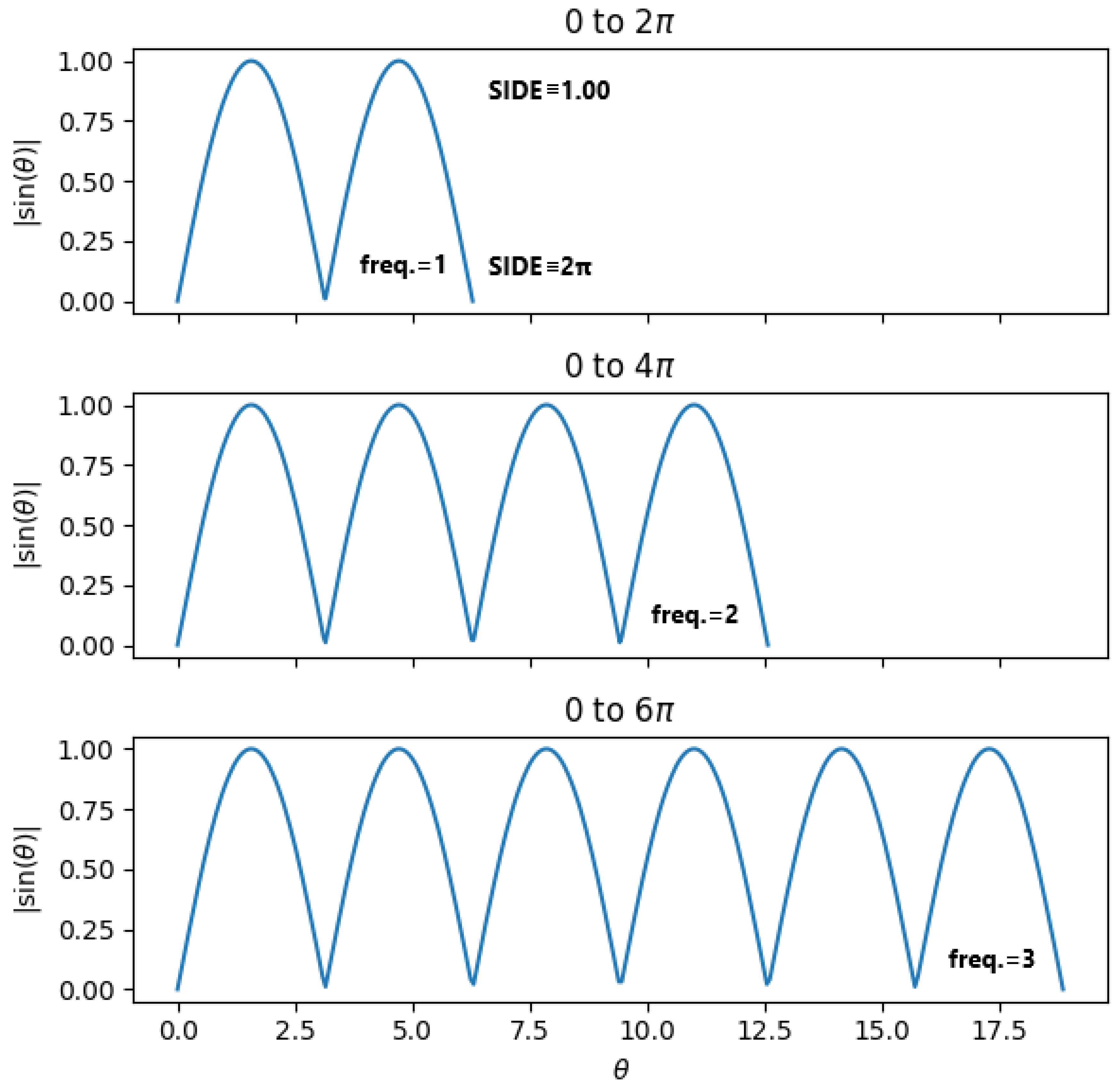
Figure 2.
Sine cloud. Two shells with points distribution proportional to the sine are shown here. The outer shell first octant was removed to expose the inner shell.
Figure 2.
Sine cloud. Two shells with points distribution proportional to the sine are shown here. The outer shell first octant was removed to expose the inner shell.
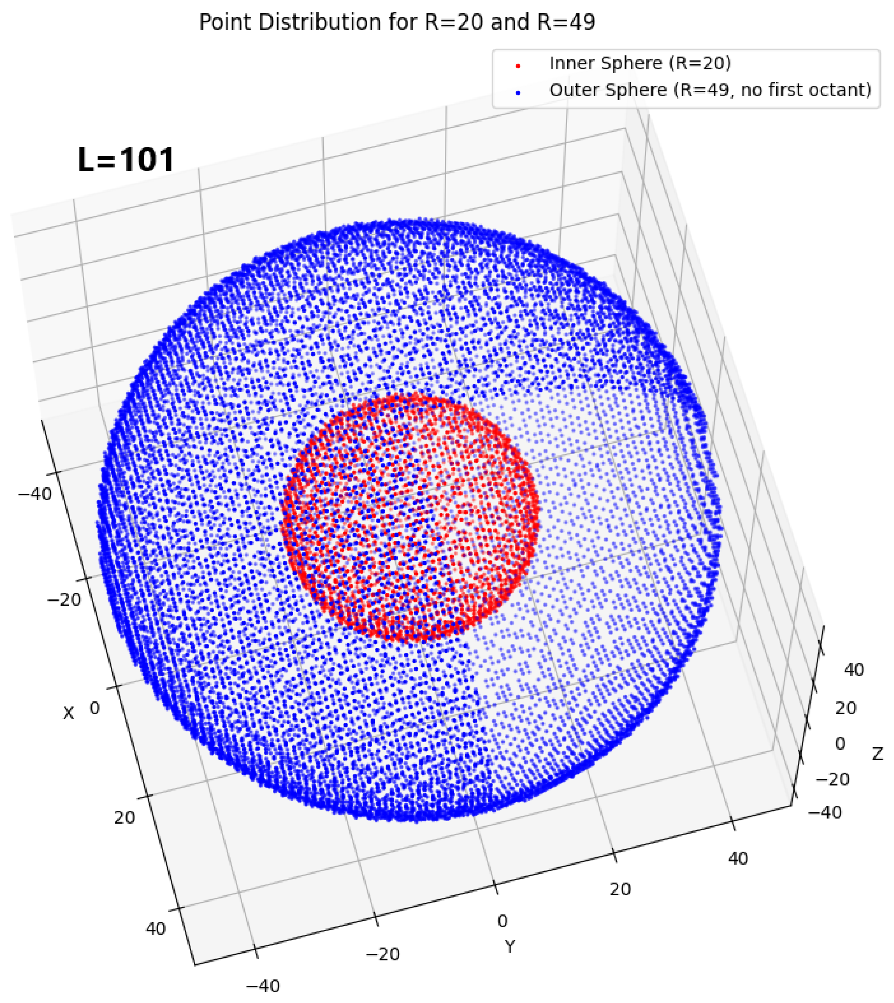
Figure 3.
The canonical spiral. The canonical Archimedean spiral spans an angle of radians. It is replicated across each base using a rotation matrix , inducing light polarization patterns.
Figure 3.
The canonical spiral. The canonical Archimedean spiral spans an angle of radians. It is replicated across each base using a rotation matrix , inducing light polarization patterns.
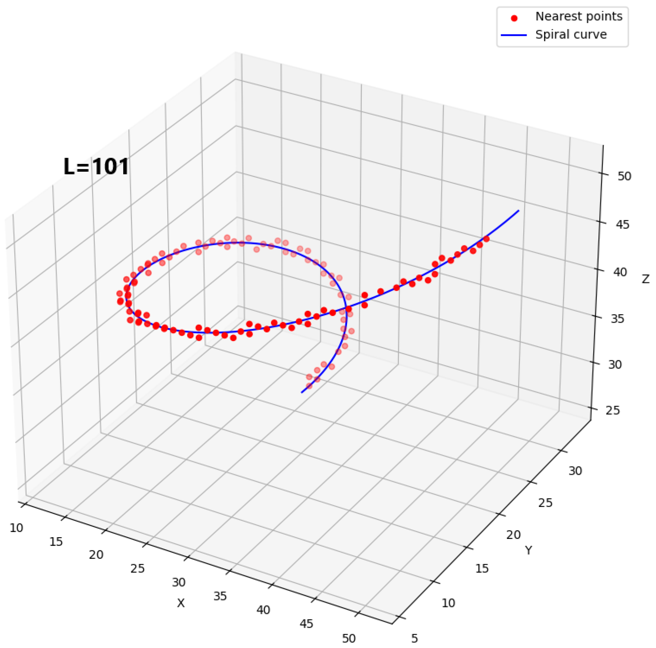
Figure 4.
Color combination. Possible combinations of colored fragments are shown, where (anti)quark fragments are marked q and , (anti)neutrinos are and , gluons are g, and photons are . Since half the gluon fragments are right handed, they are shown as photons. The cells marked as blue, if having electric charge , may form an up quark fragment in Orbis.


Table 1.
Cell structure.
| Name | Type | Symbol | Obs. |
|---|---|---|---|
| Physical properties | |||
| charge | B6 | ch | bits q, , , , , |
| pole | B | p | linear motion direction bit |
| meta-pole | B | rotation spiral bit | |
| affinity | N | a | groups bubbles into particles |
| position | V | spatial coordinates | |
| Wavefront | |||
| Euclidean distance | DN | d | for spherical constraint |
| sine mask | B | s | fixed half-period mask bit |
| wavefront tick | DN | t | light clocking |
| sine timing | DN | independent time for sine (arc) | |
| sine phase | B | a bit indicating the sign of the sine | |
| Operational variables | |||
| relocation offset | V | c | determines reissue address |
| housekeeping tick | DN | k | timeless clocking |
| collapse flag | B | hints collapse | |
| frequency counter | N | f | superposition counter |
The formatted bit string is valid for all cells, where N represents a natural number, DN a double natural number, V a three-dimensional natural vector, and B a boolean. The conventions for the values false and true for each charge bit are as follows: q: +, -; : [O]rbis, [D]ark; : [R]ight, [L]eft; : [B]lue, anti[]lue; : [G]reen, anti[]reen; : [R]ed, anti[]ed (see Section 2.1).
Table 2.
Charge combination
| Fragment | Type | Orbis | Umbra | Obs. |
|---|---|---|---|---|
| Gluon | Pair | 3,6760.0 | 3,6760.0 | |
| Up quark | Pair | 42.0 | 42.0 | |
| Down quark | Single | 10.0 | 10.0 | |
| Electron | Single | 31.0 | 31.0 | |
| Photon | Pair | 20.0 | 20.0 | |
| Graviton | Pair | 12.0 | 12.0 | |
| Z boson | Pair | 24,592.0 | 18,416.0 | |
| W boson | Pair | 6,122.0 | 12,294.0 | |
| Neutrino | Pair | 6,082.0 | 6,082.0 | |
| Antiup | Pair | 2.0 | 2.0 | |
| Antielectron | Single | 1.0 | 0.0 | |
| Antiquark | Single | 0.0 | 0.0 | |
| Leftover | Single | 24,624.0 | 24,620.0 | Adds to dark matter |
| Total | 196,602.0 | |||
A total of 196,608 bubbles were randomly combined into several million attempts in a small program focused on charges alone (See Section 9 for more details).
Disclaimer/Publisher’s Note: The statements, opinions and data contained in all publications are solely those of the individual author(s) and contributor(s) and not of MDPI and/or the editor(s). MDPI and/or the editor(s) disclaim responsibility for any injury to people or property resulting from any ideas, methods, instructions or products referred to in the content. |
© 2025 by the authors. Licensee MDPI, Basel, Switzerland. This article is an open access article distributed under the terms and conditions of the Creative Commons Attribution (CC BY) license (http://creativecommons.org/licenses/by/4.0/).
Copyright: This open access article is published under a Creative Commons CC BY 4.0 license, which permit the free download, distribution, and reuse, provided that the author and preprint are cited in any reuse.


