Climate Characterization and Prediction in Vulnerable Regions of the Ecuadorian Amazon

1. Introduction

Since the Earth’s formation, climatic variations have occurred, evidenced through paleoclimate, which were documented in the 19th century ([1]). Initially, scientists did not recognize differences between prehistoric and modern climates; however, geological evidence demonstrated that climate changes are natural processes of the climate system, which does not remain constant over time ([2]).

Current climate change, according to various sources, is primarily attributed to the increase in greenhouse gas (GHG) emissions since the Industrial Revolution, driven by human activities such as the burning of fossil fuels and deforestation ([3]). The UN indicates that these human activities are the main cause of global warming, which has caused an increase of approximately 1.0°C since pre-industrial levels, with projections suggesting an increase of up to 1.5°C between 2030 and 2052 ([4]). This global warming leads to a transformation in climatic zones, generating drier and less cold climates ([5]).

According to the IPCC [6], climate change is causing a series of impacts, such as intense droughts, water stress, heat waves, and negative effects on agriculture ([7]). It is estimated that climate exposures will double between 1.5°C and 2°C, which will expand the land area affected by these changes ([8]). Furthermore, climate change accelerates soil degradation, a non-renewable resource essential for food and raw material production ([9]). Soil regeneration is a slow process, and climate change intensifies the speed and magnitude of this degradation, leading to the emergence of new deterioration patterns ([10]).

Soil degradation has repercussions that transcend the Earth’s surface, as it affects both marine and freshwater systems and impacts people and ecosystems distant from the degradation sites ([11]). These effects represent a significant threat to global food security, given that climate change can alter soil organic matter, crops, vegetation, and increase water scarcity, which would negatively affect agricultural systems ([12]).

Regarding water resources, the effects of climate change vary depending on the region; while some areas experience increases in precipitation and runoff, others face significant reductions, exacerbating water scarcity and pressure on these resources. Additionally, temperature variation can affect water quality by increasing sediment, nutrient, and contaminant loads in river flows, altering water quality and aquatic ecosystems ([13]).

In the province of Orellana, specifically in the cantons of El Sacha and Loreto, there is a scarcity of research on climate change, which highlights the need to characterize the various climatic variables in these geographical areas over time. This analysis is crucial to understand local climate behavior, predict future changes, and make informed decisions in areas such as agriculture, water resource management, and natural disaster mitigation. Knowing local climatic conditions can help farmers select suitable crops, schedule planting and harvesting, and apply climate-adapted agricultural practices. Moreover, this knowledge is essential for managing the environmental impact of human activities and promoting more sustainable practices.

To carry out this characterization, methods of climatic data collection were used, along with the formulation of hypotheses, statistical tests, and the use of tools such as Python for graphical representation of the results. Furthermore, physicochemical and microbiological analyses of water, as well as physicochemical analyses of soil, were performed to determine if there are climatic differences between the cantons of El Sacha and Loreto and how climatic variables impact soil and water parameters. The study’s objective is to understand how these variables influence agriculture and the environment, providing a basis for more sustainable management strategies. It is expected that the research results will benefit policymakers, agricultural planners, and local communities, promoting sustainable practices and the preservation of natural resources.

Meteorology is a scientific discipline that studies the atmosphere and meteorological phenomena, such as rain, wind, and rainbows, as well as larger-scale phenomena, such as pressure systems and cyclones. These phenomena vary in duration according to their scale, from wind gusts lasting seconds to pressure systems that can last weeks. Key parameters in their analysis include air temperature, atmospheric pressure, relative humidity, wind speed and direction, and precipitation ([14,15]). The objective of meteorology is to understand atmospheric conditions and the processes that generate them, which is crucial for weather interpretation and forecasting ([16]).

Climatology, unlike meteorology, studies the temporal average of the atmospheric state in a region over extended periods, typically 30 years ([17,18]). It uses similar variables to meteorology, such as temperature and precipitation, to characterize the climate of a specific location ([19]).

The Earth’s climate system is composed of five subsystems: the atmosphere, the hydrosphere, the cryosphere, the lithosphere, and the biosphere, which interact dynamically, exchanging mass, energy, and momentum. This dynamic equilibrium generates the climate and gives rise to its inherent variability ([20,21]).

Climate change has been primarily driven by the increase in greenhouse gases (GHGs) due to human activities, such as the emission of carbon dioxide and methane. These gases intensify their impact on the global climate system ([22,23]). The effects of climate change include an increase in global temperature and alterations in precipitation patterns, affecting agriculture and water resources ([24,25]).

Water, vital for life, covers 70% of the Earth’s surface and exists in three states: solid, liquid, and gaseous. Climate change threatens both the availability and quality of water resources, exacerbating extreme weather events and altering aquatic ecosystems ([8,26]).

The research question guiding this study is: Are there statistically significant differences in the climatological variables (solar radiation, temperature, pressure, relative humidity, precipitation, wind speed, and wind direction) recorded between the geographical locations of El Sacha and Loreto?

2. Materials and Methods

This research employed a technical-explanatory and quantitative methodology, which combined the collection of historical meteorological data (1998-2021) with physical-chemical and microbiological analyses of water, as well as physical-chemical analysis of soils. The process was structured in two clearly differentiated phases: a field phase and an experimental phase, each with its specific procedures.

Firstly, during the field phase, water and soil sampling was carried out following protocols established by specialized entities. For soil sampling, the guidelines defined by the National Institute of Agricultural Research (INIAP) were applied. Likewise, water sampling was executed in accordance with Ecuadorian Technical Standards (NTE INEN), always in strict compliance with current environmental regulations in the country.

Subsequently, in the experimental phase, the collected data were processed and analyzed using advanced computational tools, including statistical software packages and programming languages. Descriptive and quantitative analyses focused on ensuring a precise and reliable interpretation of the information. It is important to note that water analyses were performed in specialized laboratories, while soil samples were processed externally in certified facilities for this type of study.

Additionally, to support the theoretical foundations of the research and ensure a rigorous approach, the PRISMA (Preferred Reporting Items for Systematic Reviews and Meta-Analyses) methodology was applied to conduct a systematic literature review. In this stage, an exhaustive search was performed in recognized databases, such as Web of Science, ACM, IESS, Scopus, among others. This initial search identified a total of 478 records. The inclusion criteria considered only articles in English published from the year 2020 onwards, while the exclusion criteria discarded publications prior to that date and undergraduate theses (see Figure 1).

After the purification and evaluation process, 58 relevant articles were identified and finally used as a theoretical foundation in this research. These documents represented a key source to consolidate the analysis and support the study’s conclusions.

This integrated approach combined established scientific methodologies with contemporary technologies, thereby ensuring the acquisition of accurate and representative results pertaining to climatic variables, water quality, and soil condition The research was carried out in the province of Orellana, situated in the northeastern region of Ecuador, within the Amazon basin. The study sites comprised the Agroforestal farm, located within the San José de Dahuano parish of the Loreto canton, and the Chela farm, situated in the urban parish of Joya de los Sachas, belonging to the canton of the same name.

The Loreto canton, established on August 7, 1992, encompasses an area of 214,637.51 hectares and is bordered to the north by the El Chaco canton, to the south by the Tena canton, to the east by the Francisco de Orellana canton, and to the west by the Quijos and Archidona cantons. This canton has a population of 24,579 inhabitants, distributed across five rural parishes and one urban parish, which serves as both the parish and cantonal administrative center. The San José de Dahuano parish, the focus of this study, incorporates 42 communities ([27]). The principal economic activities in Loreto encompass food services, mining and quarrying operations, followed by agriculture, livestock farming, aquaculture, silviculture, and fishing, among other pursuits (Figure 2).

Concurrently, the Joya de los Sachas canton is located to the northwest of Orellana province, bordering to the north the Lago Agrio and Cáscales cantons of Sucumbíos province, to the south the Francisco de Orellana canton, to the east the Shushufindi canton, also of Sucumbíos province, and to the west again the Francisco de Orellana canton. With a population of 67,732 inhabitants, this canton is composed of eight rural parishes: Enokanqui, Lago San Pedro, Pompeya, Rumipamba, San Carlos, San Sebastián del Coca, Tres de Noviembre, Unión Milagreña, and Joya de los Sachas, which functions as the cantonal administrative center. The prevailing economic activities encompass agriculture, hunting, silviculture, construction, and fishing ([28]).

2.1. Methodological Process for the Analysis of Climate Variables

2.1.1. Data Base Selection

Geostationary satellite data were employed for this research due to the absence of INAMHI meteorological stations within the study area (INAMHI, 2022). In accordance with the WMO Manual on the Global Data Processing and Forecasting System (2019), satellite-derived data are required to adhere to specific control criteria, including, inter alia, satellite operational status and a minimum threshold of observations. For the purpose of data acquisition, several platforms were utilized, including:

• National Solar Radiation Database (NSRDB): This database encompasses hourly and 30-minute meteorological data spanning from 1998 to 2021 for Ecuador, with a spatial resolution of 4 km by 4 km, accessible without charge via the NSRDB Viewer or API ([29]).
• NASA Giovanni: A web-based platform facilitating access to atmospheric data derived from remote sensing instruments with high temporal resolution. This platform offers a range of visualizations and analyses of parameters such as aerosols, atmospheric temperature and humidity, and precipitation, as well as output from assimilation models ([30]).
• Prediction of Worldwide Energy Resources (POWER): This resource provides satellite-derived data pertaining to solar energy and meteorology, which are of utility to industries such as agriculture. Solar and meteorological data are derived from models such as NASA’s MERRA-2 and are subject to daily updates ([31]).

These platforms furnished the requisite data for climatic analysis at the designated study locations, in compliance with the standards established by international bodies.

2.1.2. Data Download

In accordance with WMO guidelines (2017), the computation of climatic averages necessitates the availability of at least 80% of the data (24 out of 30 years), with no consecutive missing values spanning three years. Satellite-derived irradiance data and nighttime data are excluded due to the absence of corresponding terrestrial measurements and potential inaccuracies arising from stray irradiance. The data utilized encompasses the period from 1998 to 2021, employing a 24-hour interval.

To procure data from the NSRDB, access is gained to the viewer on NSRDB, whereby the study area is selected using GPS coordinates. Subsequently, the relevant dataset, parameters, and time interval are specified. Finally, an email address is provided to facilitate data delivery.

The utilization of the EarthData platform necessitates a registered EarthData account. The required time series, period, and coordinates are selected, and the appropriate parameters are designated. Data download is initiated upon clicking "Plot Data" and selecting the CSV file format.

Accessing the POWER platform involves navigating to POWER, selecting the "Agroclimatology" community, the temporal scale, and the relevant coordinates. Subsequently, the download format (CSV) is specified, the desired parameters are selected, and the pertinent information is retrieved upon clicking "Submit".

2.1.3. Data Processing, Sorting and Storage

All data downloads were executed in CSV format, thereby enabling subsequent data classification for processing purposes. For this undertaking, Microsoft Excel software was employed, which facilitates the importation of data from text-based files. This program allows for the selection of the appropriate delimiter for column separation, a crucial feature when dealing with substantial data volumes, thus ensuring their proper organization and management.

Subsequently, each of the variables corresponding to the 48-year data period was scrutinized to identify potential anomalies. During this review process, missing data were imputed, substituting those values that were unavailable. As an illustration, in the case of the NSRBD platform, wind speed values exhibiting gaps were comprehensively replaced with values obtained from NASA GIOVANNI, thereby ensuring data continuity and consistency for subsequent analyses.

2.1.4. Programming Language Selection

Python is a general-purpose programming language, recognized for its efficiency, manageability, and simplicity, which facilitates its learning and adoption. This language was developed in the early 1990s by Guido van Rossum, who incorporated features from previous programming languages. As a result, Python is widely used on various platforms and operating systems, standing out for its versatility. Furthermore, its development is under an open-source license approved by the Open Source Initiative (OSI), which allows its free distribution and use, even in commercial applications ([32]).

2.1.5. Data Description

The purpose of Box’s M test is to evaluate whether the covariance matrices of the dependent variables are homogeneous among the study groups. In this case, the result obtained was statistically significant (p= 0.000 < 0.05), which shows the absence of homogeneity in the covariance matrices. This implies that the variances and covariances of the dependent variables present significant differences between the analyzed locations (El Sacha and Loreto) and the considered periods (see Table 1).

Although this condition may represent a violation of one of the fundamental assumptions of MANCOVA analysis, it is possible to continue with the interpretation of Pillai’s trace. This statistic is recognized for its robustness against the lack of homogeneity in covariance matrices, which allows for the validation of the results under these conditions.

The Levene’s test is used to determine whether the variances of the dependent variables are equal among the different groups analyzed. In this case, the significance values (p < 0.05) obtained for all dependent variables show that the variances are not homogeneous. This result allows concluding that the observed differences between the locations and time periods have a statistically significant effect on the distributions of the climatic variables (see Table 2)

2.2. Process for Soil and Water Quality Analysis

The Table 3 shows the geographic coordinates of the sampling points, accompanied by the number of samples taken at each location. These points were distributed in the two studied locations, Loreto and Joya de los Sachas, covering both soil and water samples. This experimental design allows for detailed and representative analyses of the physicochemical and microbiological characteristics of both regions, allowing a comparative evaluation of the environmental conditions present in each one.

The table summarizes the methodologies employed within the laboratory for the analysis of the soil’s physicochemical parameters. Each technique implemented conforms to international standards, such as potentiometry, utilized for the determination of pH, and colorimetry, applied in the quantification of macronutrients. These methodologies are essential for the attainment of reliable and precise results, which is of paramount importance for the appropriate assessment of soil quality on the experimental farms. These procedures ensure analytical consistency and data comparability, thereby enabling a precise diagnosis of the edaphic conditions (see Table 3)

These processes ensure a comprehensive and exhaustive analysis of the collected samples, thereby enabling a precise evaluation of the soil’s physicochemical and microbiological properties. The application of techniques such as potentiometry, conductimetry, and the Bouyoucus method, inter alia, provides key data for comprehending not only the soil’s structure and composition but also its water retention capacity, pH levels, and the availability of essential nutrients. Concomitantly, the analysis of organic matter and micronutrients is of fundamental importance for evaluating soil fertility and its suitability for cultivation.

The integration of these methodologies facilitates a detailed characterization of soil conditions within the studied areas, thereby facilitating the identification of potential limitations or necessary interventions. Based on this information, more efficacious strategies can be formulated to enhance soil quality, optimize agricultural utilization, and safeguard the surrounding ecosystems. Furthermore, microbiological analysis complements the evaluation by furnishing information regarding the soil’s biological activity, a crucial aspect for comprehending decomposition processes and nutrient cycles that exert a direct influence on agricultural productivity and environmental sustainability (see Table 4).

Consequently, the implementation of these processes not only enhances the precision of environmental diagnoses but also promotes the development of more sustainable agricultural practices adapted to local conditions.

2.3. Water Sampling and Monitoring Process

The Table 5 presented herein includes the parameters employed in the physicochemical analyses of water, as well as the standardized analytical methods utilized for each. The methods enumerated are expressed in coded form, corresponding to international standards stipulated in current regulations. These methods are predicated on widely recognized procedures, including titrations, colorimetric assays, and spectrophotometries, which facilitate the precise measurement of various constituents present within the water, such as pH, sulfates, and arsenic, inter alia. This methodology ensures the reliability and precision of the results obtained, thereby ensuring adherence to the quality criteria established for monitoring purposes.

For the determination of hardness, 25 ml of sample were used, to which 1 ml of KCN, 2 ml of buffer with pH 10 and a pinch of Eriochrome black indicator T were added. Subsequently, it was titrated with EDTA, following the procedure described by APHA, AWWA and WPCF.

In the case of sulfates, the corresponding test was first selected in the equipment. Then, the sample was prepared, consisting of filling a one-inch square cuvette with 10 ml of sample up to the mark, to which a sachet of powdered Sulfaver reagent was added. The mixture was stirred in rotation and then the timer on the equipment was selected to start the reaction period. For the blank, a cuvette with 10 ml of distilled water was used. Once the reaction time was over, the outside of the blank cuvette was cleaned well and placed in the cuvette holder with the mark facing the front. Subsequently, the equipment was calibrated by selecting zero on the display. Finally, the cuvette with the sample was placed in the same way as the blank and the measurement was performed.

For the determination of iron, the corresponding test was selected and the sample was prepared by filling a cuvette with 10 ml of sample. Ferrover’s reagent powder was added and stirred in rotation. After mixing, if iron was present, an orange color was observed. The reaction period was selected on the instrument display. For the blank, 10 ml of distilled water was used. Once the timer beeped, the blank cuvette was placed and the instrument was calibrated by selecting zero. Then, the cuvette with the sample was placed and the measurement was performed.

For nitrites, the test was selected on the equipment and the sample was prepared with 10 ml in a cuvette. Then, the reagent was added and stirred in rotation. After stirring, the timer was selected, and if nitrite was present, the sample turned amber. For the blank, another cuvette with 10 ml of distilled water was used. Once the timer sounded, the cuvette was cleaned and placed in the equipment for calibration. Then, the sample was added and the measurement was performed.

The Table 6 presents the materials and equipment requisite for the microbiological analysis of water. Reagents, such as lactose broth, crystal violet, and Lugol’s solution, are of fundamental importance for the performance of staining procedures and microbiological assays, specifically in the identification of fecal coliform bacteria. These reagents facilitate the differentiation and precise observation of the samples. With respect to equipment, the incubator, laminar flow cabinet, and optical microscope are included, which are indispensable for the handling and analysis of the samples. This equipment ensures the appropriate conditions for bacterial isolation and observation, thereby ensuring the reliability and accuracy of the results obtained.

2.4. Process for Microbiological Analysis of Water

For this process, the standardized multiple-tube fermentation technique (Most Probable Number or MPN) from Standard Methods for the Examination of Water and Wastewater was used. This method is divided into two phases. In the presumptive phase, to determine the presence of coliform bacteria, the MPN technique, consisting of serial ten-fold dilutions, was employed. Prior to sample collection, materials were washed with neutral detergent and distilled water, and subsequently sterilized in a hot air oven. Flasks were autoclaved to ensure proper disinfection. Once the samples were stored in the laboratory refrigerator, the lactose broth was prepared, with necessary calculations made to accommodate the four samples. Two concentrations of lactose broth were used in this process.

The lactose broth was prepared using 5.2 grams of lactose broth medium in 200 mL of distilled water for 20 tubes of concentrated broth. For the single concentration, 5.2 grams of lactose broth medium were used in 400 mL of distilled water for 40 tubes. 500 mL and 300 mL flasks were used to prepare the broths, and inverted Durham tubes were placed inside to detect gas production. After preparing the broths, they were autoclaved for 15 minutes. Once cooled, the concentrations were separated using a test tube rack.

The concentrations were transferred to the UV fluorescence chamber. Before placing the material in the chamber, the surface was disinfected with a cloth and Lugol’s solution, and 75%-90% alcohol was sprayed onto the materials. Using a 10 mL manual pipette, 10 mL of sample were added to the concentrated broths, and 1 mL and 0.1 mL were added to the single concentrations using automatic pipettes. Although an inoculation loop could have been used, automatic pipettes were chosen for their practicality and efficiency.

In the confirmatory phase, after 48 hours, the presumptive fermentation tubes that showed gas production or heavy growth were examined. Tubes exhibiting these signs were gently agitated. In this phase, EC medium was prepared according to a specific composition. To prepare the EC medium, 2.96 grams of EC medium were dissolved in 80 mL of distilled water. The medium was dispensed into 10 mL tubes, and inverted Durham tubes were used to confirm gas production. After autoclaving the tubes, they were allowed to cool and marked with a marker to indicate the sample volume to be used. The inoculated tubes were incubated at 44.5°C for 24 hours. Gas production in EC medium within 24 hours or less was considered a positive reaction.

For bacterial identification using Gram staining, the streak plate method was used. This method is used to isolate aerobic and facultative anaerobic Gram-negative bacilli from clinical, water, and food samples, allowing for the isolation of coliforms using a selective medium for non-fastidious bacilli. In this process, a small amount of sample is inoculated onto a solid medium, such as nutrient agar, and a series of streaks is performed to obtain isolated colonies, which are incubated and observed to identify the bacteria present.

The steps for streak plating include sterilizing the platinum loop with a Bunsen burner, inoculating the sample onto the solid medium, and rotating the Petri dish to achieve a progressive and continuous distribution of the bacteria. This procedure is repeated until isolated colonies are obtained on the plate, which are incubated and observed for bacterial identification.

Finally, for Gram staining, a microscope slide was used, to which drops of distilled water were added. After heating the slide over the Bunsen burner, a colony was taken from the sample and stained with crystal violet, rinsing with running water. Subsequently, Lugol’s iodine was applied, followed by decolorization with acetone-alcohol and a rinse with running water. Finally, safranin was applied for 15 seconds, and the slide was observed under a microscope, where Gram-positive bacteria appeared blue and Gram-negative bacteria appeared red.

3. Experiments

3.1. Temperature in the Canton of Loreto

Between 1998 and 2021, characteristic thermal patterns were identified in the temperature records. During the initial period (1998-2003), temperatures consistently ranged between 23 °C and 25 °C, with recurrent increases in early August. In the 2004-2009 interval, marked fluctuations and anomalies in the sequence were evident, such as in 2005, when temperatures experienced a substantial increase during the months of July, August, and September. In 2007, temperatures rose at the beginning of the year but showed a progressive decrease towards the later months, while in 2009 the opposite behavior occurred, with increases towards the end of the year.

The period from 2010 to 2015 presented a relative return to stability, with thermal patterns similar to those observed during the early years. However, between 2016 and 2021, significant changes in temperature dynamics were detected. These included higher initial values and pronounced decreases after May, followed by a consistent increase from August onwards. These variations could be associated with climatic and environmental factors that influence seasonal patterns and with global climate change phenomena that require further study for their understanding (see Figure 3).

The ARIMA (Autoregressive Integrated Moving Average) model is widely used for time series forecasting due to its ability to analyze sequential data over time. In this case, its application is appropriate because monthly temperature is a set of data that follows a temporal behavior, which allows predicting future values from past relationships.

Likewise, this model is capable of capturing seasonal patterns and trends, which is fundamental in temperature prediction, since it presents annual variations associated with the seasons of the year. Through the adjustment of seasonal differences, ARIMA manages to model the dependence between past values and make more accurate predictions.

$${\Phi }_p\left(B\right){(1-B)}^d{Y}_t={\Theta }_q\left(B\right){ϵ}_t$$

(1)

In developed terms, the complete equation is expressed as:

$$(1-{\varphi }_{1}B-{\varphi }_2{B}^2-\cdots -{\varphi }_p{B}^p){(1-B)}^d{Y}_t=(1+{\theta }_{1}B+{\theta }_2{B}^2+\cdots +{\theta }_q{B}^q){ϵ}_t$$

(2)

The temperature prediction for the 2022-2025 period follows the general seasonal pattern observed in historical data, with lower temperatures during the middle of the year and higher values at the extremes. The predicted temperatures remain within the range of historical observations, without registering exceptionally high or low values compared to previous years. However, a pronounced peak is observed around August, similar to patterns from some previous years, as well as a significant decrease during June and July (see Figure 4).

The dispersion of the residuals remains constant over time, indicating the absence of evident problems of heteroscedasticity, that is, non-constant variance. This suggests that the variability of the model’s errors does not change significantly in different periods, which is a favorable indicator for the stability of the model. The homoscedasticity of the residuals is an important requirement in time series modeling, since it guarantees that the predictions have a uniform precision over time. In this sense, the ARIMA(2,1,2) model adequately captures the trend of the series, which indicates that the structure of the model is appropriate to describe the evolution of the data without the dispersion of the errors compromising its performance (see Figure 5).

The majority of the residuals are concentrated in values close to 0, which indicates that the model errors are well distributed and do not present a significant systematic bias. This behavior is a favorable sign, since it suggests that the model does not make consistent errors in a specific direction. In addition, the distribution of the residuals is approximately normal, although a slight deviation is observed in the extreme values (see Figure 6).

Most of the autocorrelation coefficients are within the confidence interval (shaded in blue), which suggests that the residuals do not exhibit significant autocorrelation (see Figure 7).

3.2. Pressure in the Canton of Loreto

During the period from 1998 to 2021, a notable variability in atmospheric pressure values is observed. In the first months of each year, the pressure remains within a range of 930 to 932 hPa. Between May and July, an increase towards values close to 934 hPa is recorded, without following a clearly defined pattern. In 1998, the pressure remains constant at 930 hPa during the first months, increasing to 932 hPa from May onwards. In 1999, greater variability is observed, with a significant increase in pressure between April and August, reaching levels above 934 hPa, and then decreasing in September (see Figure 8).

During the following years, atmospheric pressure remains relatively stable, with evident seasonal variations. Between 2004 and 2009, a gradual increase is observed in the first months of the year, with values ranging between 930 and 931 hPa, reaching 934 hPa in June and July, and subsequently decreasing in November. In the period from 2010 to 2016, the pressure remains between 930 and 931 hPa, registering significant increases in June and July. Finally, between 2016 and 2021, the pressure shows an upward trend, progressively increasing from March to July, reaching a maximum value of 935 hPa.

The prediction reveals a nearly constant atmospheric pressure throughout the year, with an approximate value of 932 hPa. This behavior notably contrasts with the seasonal variability recorded in historical data. The predicted value, close to 932 hPa, falls within the range of observed historical values, although it is more aligned with the typical averages of transition months, such as April-May and September-October, than with the extreme values recorded during periods of greater variability (see Figure 9).

3.3. Precipitation in the Canton of Loreto

An analysis of rainfall recorded between 1998 and 2021 was conducted. In 1998, the year began with rainfall exceeding 0.2 mm in January, which remained between 0.2 mm and 0.3 mm until May. Subsequently, a significant decrease below 0.1 mm was observed in June. In September, rainfall increased, reaching a maximum of 0.4 mm in November, before decreasing to 0.3 mm in December(see Figure 10).

The period from 2004 to 2009 showed considerable variability in rainfall, without following a defined sequence. For example, in 2004, rainfall began below 0.2 mm in January, reaching a maximum of more than 0.5 mm in April, and then stabilizing between 0.2 mm and 0.4 mm for the remainder of the year. Subsequent years showed similar patterns of variability.

Between 2010 and 2015, greater regularity in rainfall was identified, with values fluctuating between 0.2 mm and 0.4 mm during the first months of the year, and decreasing to levels between 0.1 mm and 0.2 mm in August. Finally, the period from 2016 to 2021 showed annual variability in rainfall, with values ranging from more than 0.2 mm to less than 0.5 mm, with recorded minimums between less than 0.1 mm and 0.2 mm.

The prediction shows a general decreasing trend in average monthly precipitation over the four years analyzed. In this regard, each successive year, such as 2023, 2024, and 2025, predicts slightly lower values compared to the initial year, 2022. This decrease occurs linearly, which reinforces the idea of a stable downward pattern.

Furthermore, although the prediction attempts to reflect the characteristic seasonal pattern, with higher values at the beginning of the year and lower values towards the middle, the fluctuations are significantly less pronounced in relation to the historical data. As a result, the peaks and troughs observed in the original data are smoothed, suggesting lower seasonal variability in future years. In other words, the differences between the wettest and driest months are expected to be less marked in the projected period.

On the other hand, the predicted values generally remain within the range of historical values observed between 2016 and 2021. However, as the prediction years progress, especially from 2023 onwards, the values tend to be located in the lower part of the historical range, approaching the minimums recorded in some of those years. This reinforces the idea of a gradual decrease and reduced variability in future rainfall(see Figure 11).

3.4. Relative Humidity of the Canton of Loreto

They presented values between 92.5% and over 85%. In 2003, humidity records remained above 90%, and in December 2000, the lowest humidity was reached, although it remained above 80%.

Between 2004 and 2009, a significant decrease was observed in 2005, with a recorded humidity of 65% in August, in contrast to other years that showed values between 80% and 90%. In 2007, initial humidity levels were lower, around 80%.

Between 2010 and 2015, relative humidity records were between 90% and 95% in August, although a general decrease fluctuating between 85% and 90% was observed. The year 2010 stood out for having the lowest humidity, around 75%.

In 2016 and 2017, humidity values remained constant between 90% and 95%. Finally, between 2018 and 2021, initial humidity levels ranged between 80% and 85%, but decreased in August and September, reaching values between 75% and 80%, before returning to initial levels during the remaining months (see Figure 12).

The prediction shows a slight downward trend in average monthly relative humidity over the four projected years. However, this decrease is less pronounced compared to that observed in the precipitation prediction. Similarly to the latter, the prediction tends to smooth out the seasonal fluctuations present in the historical data, implying less variability between months. In this context, the difference between the months with the highest and lowest relative humidity is notably smaller in the future estimates. Furthermore, the predicted values, while generally remaining within the range of historical values, tend to be positioned towards the lower end of that range, particularly in the later years of the projected period. This behavior suggests that the anticipated conditions would be slightly drier compared to the observed historical average (see Figure 13).

3.5. Radiation of the Canton Loreto

Between 1998 and 2003, solar radiation ranged from 165 W/m² to 210 W/m². During this period, a decrease in radiation was observed in May and June, reaching values below 160 W/m² and 180 W/m². However, between August and October, radiation increased, registering values between 220 W/m² and 240 W/m². On the other hand, between 2004 and 2009, the first months of the year presented radiation comprised between 160 W/m² and 210 W/m², with a decrease in June reaching levels between 190 W/m² and 150 W/m². From July onwards, radiation began to increase, ranging between 190 W/m² and 230 W/m² until December (see Figure 14).

During the period 2010-2015, solar radiation presented values between 140 W/m² and 220 W/m². Until June, it remained between 190 W/m² and 160 W/m², subsequently registering an increase between 220 W/m² and 240 W/m². In 2016, an average radiation of 210 W/m² was observed, in contrast to the values recorded in the remaining years, which remained between 150 W/m² and 185 W/m² until June. It is worth noting that in 2019 radiation reached a minimum of 140 W/m². Between July and October, radiation increased, reaching 220 W/m², with September standing out with similar values.

Unlike the predictions made for precipitation and relative humidity, the solar radiation projection shows a slight upward trend over the four years analyzed. This implies that, in general, marginally higher solar radiation values are anticipated in later years (2023-2025) compared to 2022. In this context, the prediction manages to capture the general seasonal pattern, characterized by lower values mid-year and higher values towards the end; however, the fluctuations are considerably less pronounced compared to the historical data (see Figure 15).

3.6. Wind Speed of the Canton Loreto

Between 1998 and 2003, wind speeds fluctuated between 2.4 m/s and 2.6 m/s during the first months of the year, except in 2001, when the speed began at 2.8 m/s and decreased to 2.4 m/s in May. From July until the end of October, speeds ranged from 2.8 m/s to 3.0 m/s, subsequently decreasing to values between 2.6 m/s and 2.2 m/s in the last two months of the year. However, in 2000, an unusual increase was recorded in December, reaching 2.8 m/s (see Figure 16)

In the period from 2004 to 2009, wind speed varied from 2.9 m/s to 2.4 m/s in January, with 2007 being the year with the highest values in this range. During the months of July to September, speeds fluctuated between 2.7 m/s and 2.8 m/s, showing a decrease from October to December. However, in 2006, an increase was observed in December, again reaching 2.8 m/s.

Between 2010 and 2015, speeds ranged from 2.4 m/s to 2.8 m/s, showing a progressive increase throughout the days/year. During the months of June to September, speeds were in a range of 2.6 m/s to 2.8 m/s. It is worth noting that in December 2015 a significant decrease was recorded, dropping to values below 1 m/s.

Finally, in the period from 2016 to 2021, speeds remained between 2.4 m/s and 2.7 m/s, progressively decreasing from March to May, reaching values between 2.4 m/s and 2.2 m/s. However, notable exceptions were observed: in 2016, the speed increased to 3 m/s in June, while in December 2021, high values were reached again.

The prediction reveals a slight upward trend in average wind speed over the four projected years. This suggests that wind speeds for 2023-2025 will be marginally higher compared to 2022. However, it is important to note that the slope of this trend is very gentle. The most prominent feature of the prediction is the notable attenuation of variability, both seasonal and interannual. The prediction lines exhibit a smooth and almost straight behavior, indicating that the model forecasts very little variation in wind speed throughout each year and between the different years of the projected period. In fact, a virtually constant speed is predicted throughout each year, with extremely slight changes.

Regarding the predicted values, these generally remain within the range observed in the historical years between 2016 and 2021, although they tend to be located in the mid-range of this range. The occurrence of extreme values, neither very high nor very low, is not anticipated, which reinforces the idea of relative stability in wind speed throughout the projected period.

3.7. Wind Direction of the Canton Loreto

In 1998, a predominant wind direction towards the west is observed, with speeds ranging between 2.7 and 2.9 km/h, and a frequency of less than 10%. A southwest wind direction is also identified, with speeds between 2.6 and 2.7 km/h, and a frequency of less than 20%. In this same year, a frequency of 50% is present with speeds varying between 2.2 and 2.3 km/h (see Figure 18)

On the other hand, in 2008, it is observed that the predominant wind direction was towards the southwest, with frequencies of 33.3% and speeds ranging from 2.2 km/h to over 2.7 km/h. In addition, a south wind direction was recorded, with a frequency of less than 33.3%, and speeds between 2.2 and 2.6 km/h.

In 2016, greater dispersion in wind speeds is observed. The most frequent direction was towards the southwest, with 33.3% and speeds varying between 2.2 and 2.5 km/h. Regarding the west direction, a frequency of less than 20% was recorded, with speeds between 2.8 and over 3 km/h.

Finally, in 2021, it is observed that the most frequent wind direction was towards the south, with a frequency of 50% and speeds ranging from 2.2 km/h to over 3 km/h.

3.8. Temperature of Joya de los Sachas County

From 1998 to 2003, a temperature variation was recorded, ranging between 23.5°C and 26.5°C during the months of April and May. Subsequently, in June and July, the temperature experienced a decrease, reaching 22°C. However, in August, there was an increase in temperature, which continued to rise until reaching 26°C in September. Between 2004 and 2009, in the year 2005, a significant increase in temperature in May was observed, reaching 28°C, compared to the other years, whose values did not exceed 26°C in that month (see Figure 19)

During the years 2004, 2006, and 2008, temperatures were lower, reaching 22°C in the months of July and August, not exceeding 26°C during the rest of the year. In 2009, the temperature remained constant, ranging between 23°C and 25°C throughout the year. From 2010 to 2015, the year 2010 was the hottest, with initial temperatures of 25.5°C in the first months and 24°C during the coldest months, from June to August. In the following years, until May, temperatures ranged between 24.5°C and 22.5°C. Between 2016 and 2019, the temperature did not exceed 26°C and remained below 23°C in the months of June and July. In contrast, in 2020, the temperature began at 25°C during the first months, subsequently decreasing to 24°C, then increasing again from July until reaching 27°C in September

While the prediction attempts to capture the general seasonal pattern, characterized by lower temperatures mid-year and higher temperatures at the extremes, the fluctuations are notably less pronounced compared to the historical data. The peaks and troughs are smoothed out, suggesting lower seasonal variability in the prediction.

The predicted minimum temperatures do not reach values as low as those observed in some historical years, and the peaks also do not exceed the recorded maximums. Generally, the predicted values remain within the range observed between 2016 and 2021, but tend to be located in the mid-to-high portion of that range. This indicates that slightly warmer temperatures are predicted on average compared to the historical average, although without reaching the highest peaks of some years. Furthermore, the prediction lines for the years 2022 to 2025 are very close to each other, reflecting that the model predicts extremely low variability between these years (see Figure 20)

3.9. Air Pressure in the Joya de los Sachas Canton

Between 1998 and 2003, atmospheric pressure exhibited cyclical behavior. Initially, values of 969.5 mbar were recorded, which progressively increased from May to August, reaching a maximum of 971.5 mbar. Subsequently, from September onwards, the pressure returned to the initial values. However, in the year 2000, an anomaly was observed, with a significant decrease in November to 968.5 mbar (see Figure 21).

During the period from 2004 to 2009, the pressure maintained stability at 969.5 mbar in the first months until April. From May, a sustained increase was evident, which lasted until September, again reaching a maximum of 971.5 mbar.

In the years 2010 to 2015, the pressure began at 969.5 mbar and showed a notable increase in the months of May to August. Particularly, July stood out with a maximum value of 971.25 mbar. Subsequently, in the following months, the pressure returned to the initial levels.

Finally, in the years 2016 and 2017, the initial pressure was 970 mbar. During the period from May to August, high values of 972 mbar were recorded, while, in the following months, a notable increase was observed, reaching between 974 and 978 mbar towards the end of the year

The atmospheric pressure prediction reveals a marked stability over time. Generally, the prediction lines exhibit an almost horizontal orientation, with a slight downward trend that is barely perceptible on the graph. It is worth noting that the prediction model fails to capture the characteristic seasonal pattern of the historical data, as the fluctuations associated with the seasons have almost completely disappeared. This behavior results in a projection that approximates a horizontal straight line.

The predicted values remain within the range of the historical data, although they tend to be located in the mid-to-lower part of that range. This behavior is especially evident when compared to the pressure peaks recorded in some previous years. Furthermore, the prediction lines corresponding to the different years (2022-2025) are practically superimposed, which demonstrates that the model predicts virtually nonexistent interannual variability (see Figure 22).

3.10. Precipitation in Joya de los Sachas Canton

Between 1998 and 2003, hourly data was collected for one day in a month, recording rainfall in January that ranged from 0.16 mm to 0.44 mm. In March 1999, a decrease was detected, reaching 0.21 mm, while in April an increase to 0.64 mm was observed. During the following months, the rainfall followed a pattern similar to the rest of the years, with August standing out as the month with the lowest rainfall, less than 0.1 mm (see Figure 23).

In the period between 2004 and 2009, significant variations in rainfall were identified, with high levels during most of these years. The year 2005 presented a decrease in rainfall, with August being the driest month with values less than 0.1 mm. In 2006, rainfall remained between 0.3 mm and 0.4 mm.

During the years 2010 to 2015, rainfall fluctuated between values greater than 0.2 mm and less than 0.4 mm, with a decrease to less than 0.3 mm in 2010 and a notable increase to more than 0.7 mm in March 2012. In the months of August and September, rainfall was between 0.2 mm and 0.1 mm.

Finally, between 2016 and 2021, a variation in rainfall was evidenced, with levels greater than 0.7 mm between January and April 2016, and lower values, between 0.3 mm and 0.1 mm, in August and September. During this period, rainfall ranged from 0.24 mm to 0.4 mm, except in 2018, when it decreased to 0.2 mm

The prediction reflects a slight downward trend in average monthly precipitation throughout the projected period, implying that slightly lower precipitation values are estimated in later years (2023-2025) compared to 2022. Furthermore, although the model attempts to reproduce the characteristic seasonal pattern—with higher precipitation towards the beginning and end of the year and lower precipitation in the central months—the fluctuations are notably less pronounced compared to historical data. In this regard, the peaks and troughs are attenuated, suggesting lower seasonal variability in the predictions.

Likewise, the estimated maximum precipitation is lower than historical peaks, while the predicted minimums exceed some of the lowest values recorded in the past. However, the forecasted values generally remain within the historical range observed between 2016 and 2021, although they tend to be located in the mid-to-lower part of that range. This indicates a prediction of slightly lower average precipitation compared to the historical average (see Figure 24)

3.11. Relative Humidity of Joya de los Sachas

From 1998 to 2003, it is observed that in 2001 the humidity is 75% in January, unlike the other years, where the humidity is between 82% and 95%. From March to July, the humidity remains between 92.5% and 95%. In the months of August and October, the humidities vary between 80% and 90%, and in the following months, they rise to levels above 90%, reaching between 90% and 95%. An exception occurs in the year 2000, where the humidity decreases to 80% in December.

In the years 2004 to 2009, the humidities remain above 85% and up to 95%, with general stability until May. However, in 2007, the humidity is less than 85% in January, and in February a humidity of less than 75% occurs. In the month of August, lower values are observed, with 60% in 2005, less than 75% in 2007, and 85% in 2009. In the other years, the humidity remains between 90% and 95%. Finally, from September to part of December 2006, the humidity remains below 90% (see Figure 25)

The prediction shows a slight downward trend in average monthly relative humidity over the four years. This implies that, generally, slightly lower relative humidity values are predicted in later years (2023-2025) compared to 2022. Although the prediction attempts to capture the general seasonal pattern—with higher humidity at the beginning and end of the year and lower humidity in the middle—the fluctuations are much less pronounced than in the historical data. The predicted humidity peaks are lower than the historical peaks, while the predicted minimums are higher than some of the minimums observed in the historical data. This behavior suggests that the prediction smooths out seasonal variability.

Regarding the predicted values, they generally remain within the range of historical values observed between 2016 and 2021, but tend to be located in the mid-to-lower part of that range. This suggests that, on average, slightly lower relative humidities are predicted compared to the historical average. Finally, the prediction lines for the different years (2022-2025) are very close to each other, indicating that the model predicts very low variability between these years (see Figure 26).

3.12. Radiation of Joya de los Sachas Canton

From 1998 to 2003, solar radiation is found to be between 220 and 188 W/m². During the months of May, June, and July, there is a decrease in values, ranging from 160 to 145 W/m². In the months of August, September, and October, greater solar radiation is observed, with values ranging from 220 to 240 W/m² (see Figure 27).

In the period from 2004 to 2009, variations are recorded in the months of January, February, March, and April, with radiation ranging from 150 to 220 W/m². In 2007, radiation of 140 W/m² stands out in the month of June, this being the lowest value of the period. In the months of August, September, and October of those years, an increase in radiation is observed, reaching up to 220 W/m².

In the period from 2010 to 2015, solar radiation is found to be between 130 and 217 W/m², with a notable variation in the month of January. In 2015, an increase is observed in February, with 180 W/m², unlike the other years, which show a decrease in radiation. The years 2016 and 2017 present a higher average of solar radiation.

In 2018, radiation of 110 W/m² is observed in June, while in 2019 an increase is recorded in June, reaching 130 W/m². Finally, in the years 2020 and 2021, the radiation shows less variation, remaining between 180 and 197 W/m² from January to August, and experiencing an increase in September, with values ranging from 219 to 220 W/m²

The prediction indicates a subtle upward trend in average monthly solar radiation across the projected four-year period, suggesting that slightly higher solar radiation levels are generally anticipated in 2023-2025 compared to 2022. While the prediction aims to reflect the typical seasonal cycle, characterized by lower solar radiation during the mid-year months and higher radiation at the beginning and end of the year, the observed variations are considerably less pronounced than those recorded historically. The troughs, or minimum radiation levels, are not as deep as those seen in previous years, nor do the radiation peaks reach the same heights. This smoothing effect suggests a reduction in predicted seasonal variability. In general terms, the predicted values remain within the historical range observed from 2016 to 2021, though they tend to cluster around the mid-range. Consequently, extreme high or low values are not anticipated, but rather intermediate values are projected (see Figure 28)

3.13. Wind Speed of the Joya de los Sachas Canton

From 1998 to 2003, wind speeds were consistently between 1.7 m/s and 1.8 m/s from April to June. However, speeds increased from July to September, reaching 2 m/s to 2.3 m/s. In the final months of the year, speeds decreased again, ranging from 1.8 m/s to 2.2 m/s. During the 2004-2009 period, January saw speeds between 1.8 m/s and 2.2 m/s, with increases up to 2.3 m/s observed through April. From June to September, speeds remained elevated, fluctuating between 2 m/s and 2.3 m/s (see Figure 29)

Between 2010 and 2015, wind speeds generally stayed between 1.8 m/s and 2 m/s year-round, except for 2014. In 2014, speeds ranged from 1.9 m/s to 2.4 m/s in the early months, with a drop to 1.4 m/s in November. August and September 2014 also saw higher speeds, reaching 2.2 m/s.

Finally, from 2016 to 2021, January wind speeds were between 1.70 m/s and 2 m/s. April and May saw a decrease to 1.6-1.7 m/s. Starting in June, speeds increased, reaching 1.8 m/s to 2.1 m/s.

The prediction indicates a subtle upward trend in average monthly wind speed across the four-year projection, suggesting marginally higher wind speeds are generally expected from 2023 to 2025 compared to 2022. However, this trend is minimal, implying that any increases in wind speed are unlikely to be substantial. Despite this slight upward inclination, the prediction essentially fails to capture the weak seasonal pattern present in the historical data. Indeed, seasonal fluctuations have been almost entirely eliminated, indicating a lack of significant intra-annual variability. The resulting prediction lines are nearly flat, further emphasizing the absence of seasonal trends in the forecast.

The predicted values generally fall within the range of historical data from 2016 to 2021, though they tend to cluster around the mid-range of that data. Extreme high or low wind speeds are not projected; instead, the model predicts more moderate, consistent values. Moreover, the prediction lines for the different years (2022-2025) are extremely close, almost overlapping, which clearly demonstrates that the model anticipates virtually no year-to-year variation, reflecting a uniform wind speed profile across these years (see Figure 30).

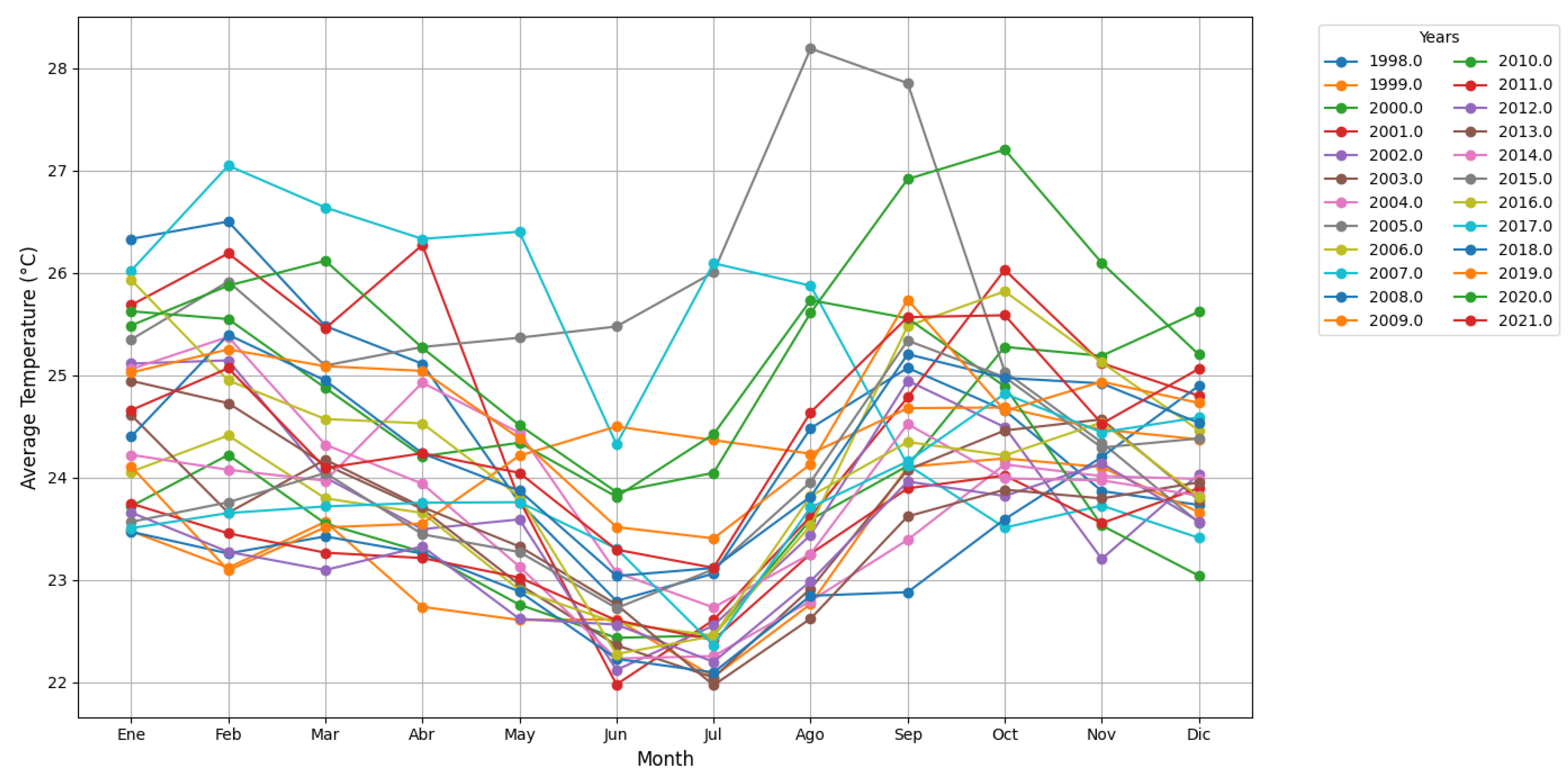
3.14. Wind Direction of the Joya de los Sachas Canton

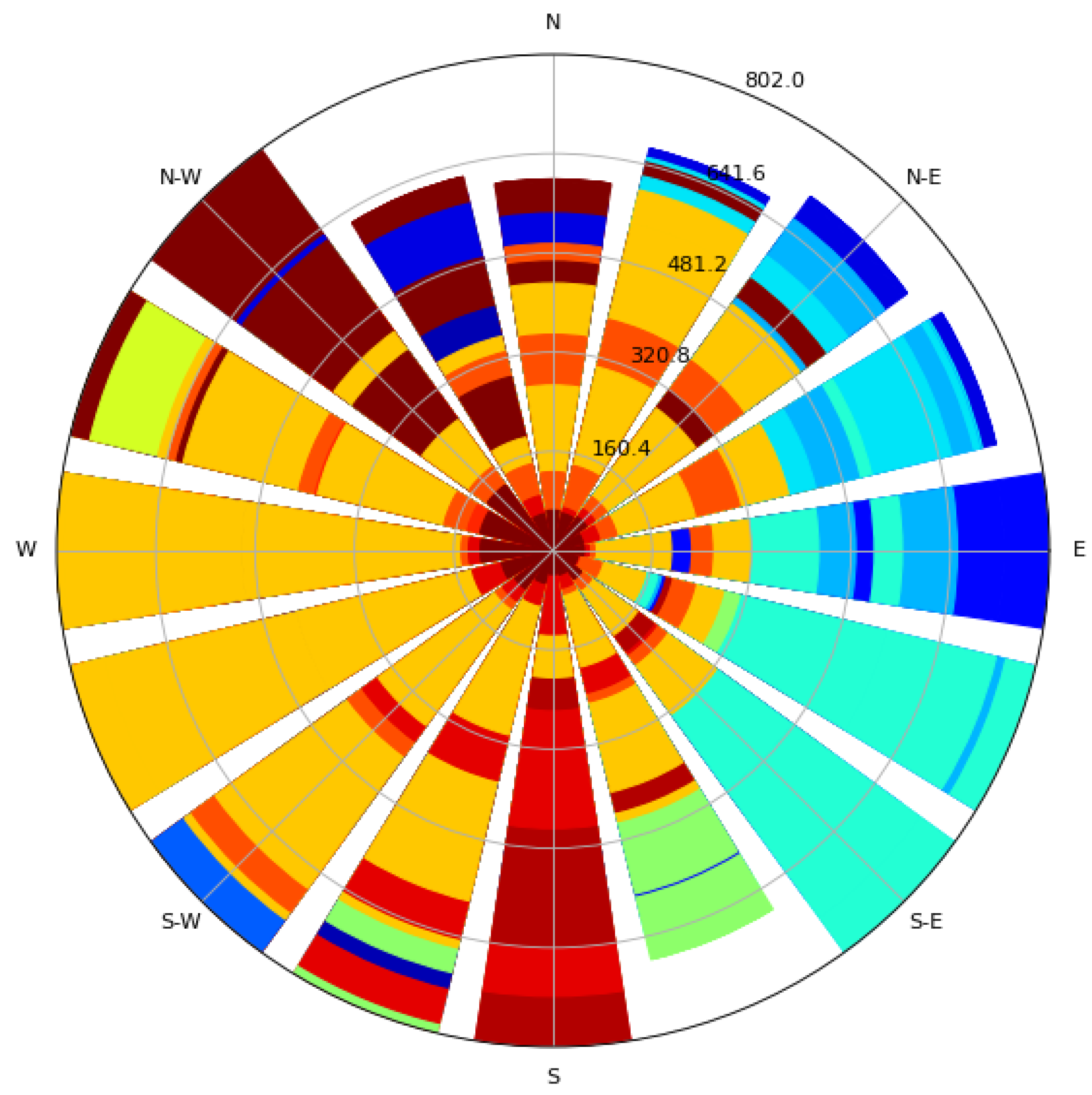
Between 1998 and 2003, the wind direction during the first month varied between 120° and 190°. From May to August, the direction consistently stayed between 220° and 240°, shifting to between 120° and 210° from October to December. During the 2004-2009 period, changes in wind direction are noticeable. A significant shift is seen in 2008, with the direction consistently at 240° from June until early October. In 2005, the wind direction remained remarkably stable between 140° and 160° throughout the year. 2007 saw a change in direction, varying from 150° to 190° (see Figure 31)

In 2010, the wind direction showed more rapid fluctuations, varying between 170° and 200°. In subsequent years, the directions started to stabilize, generally ranging from 220° to 240° from June to September. Between 2016 and 2021, and specifically in 2018, the wind direction began at 210°, contrasting with the other years, which started between 140° and 180°. This pattern highlights a distinct behavior in 2018 compared to other years in the period.

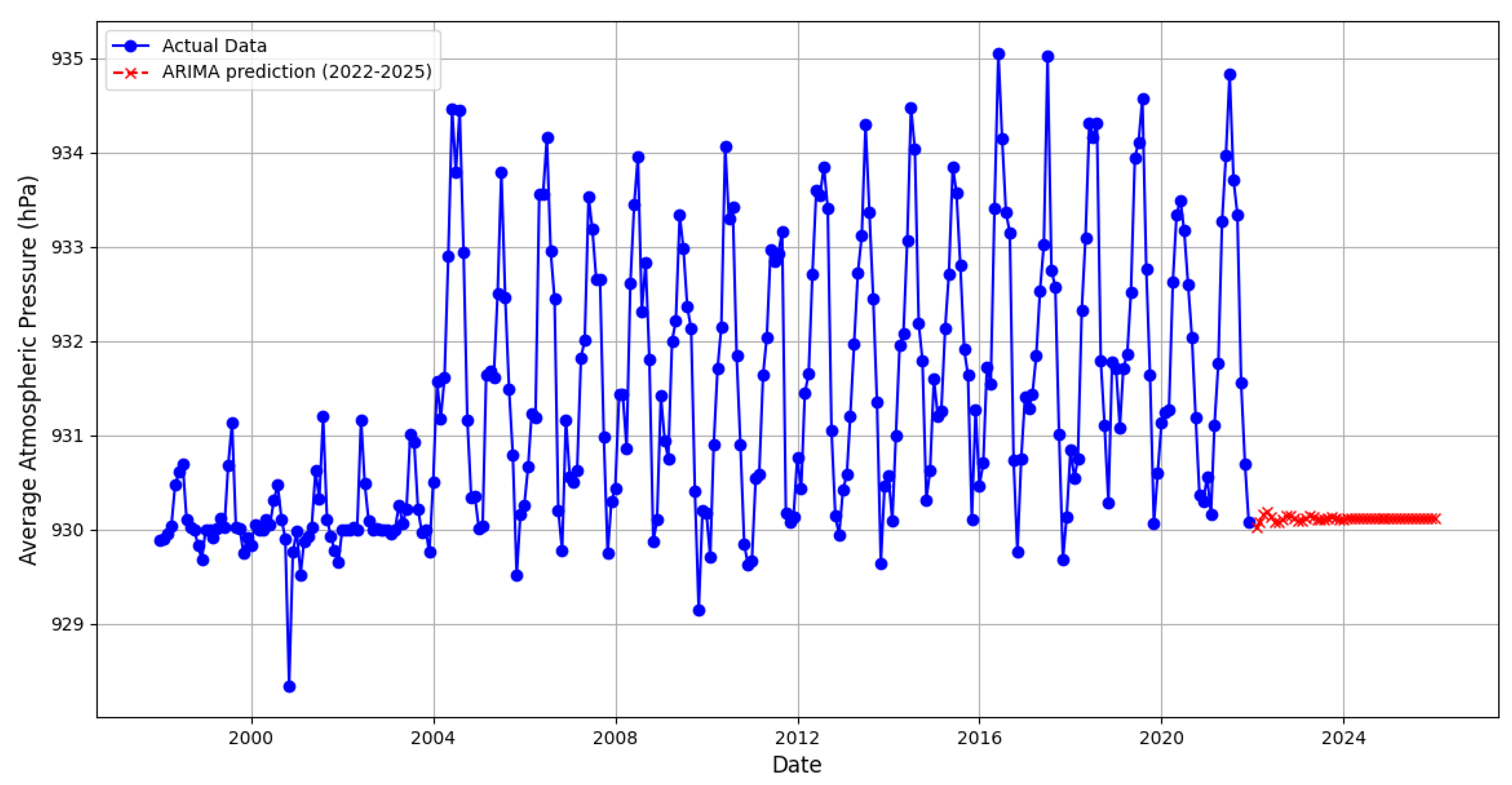
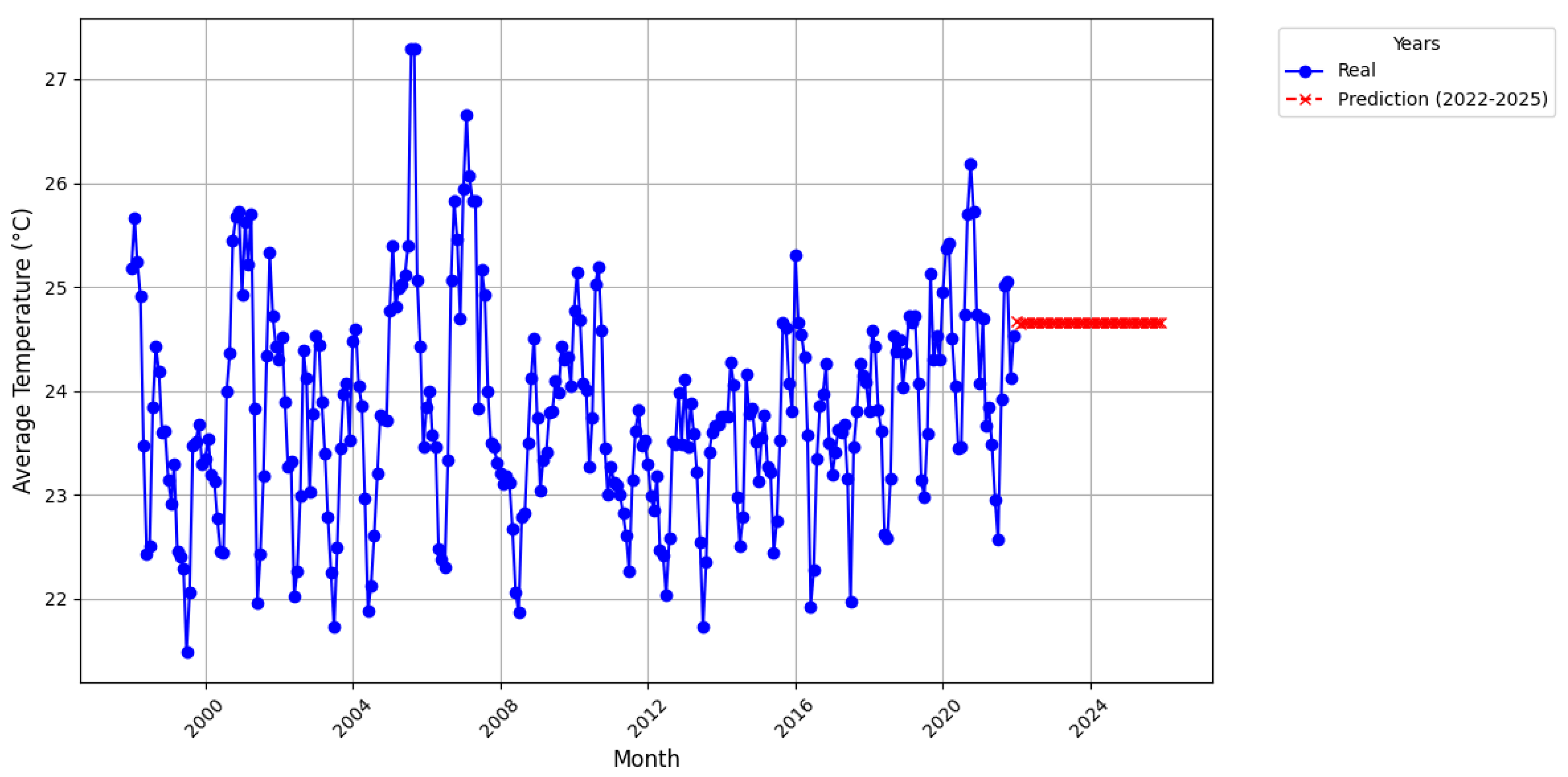
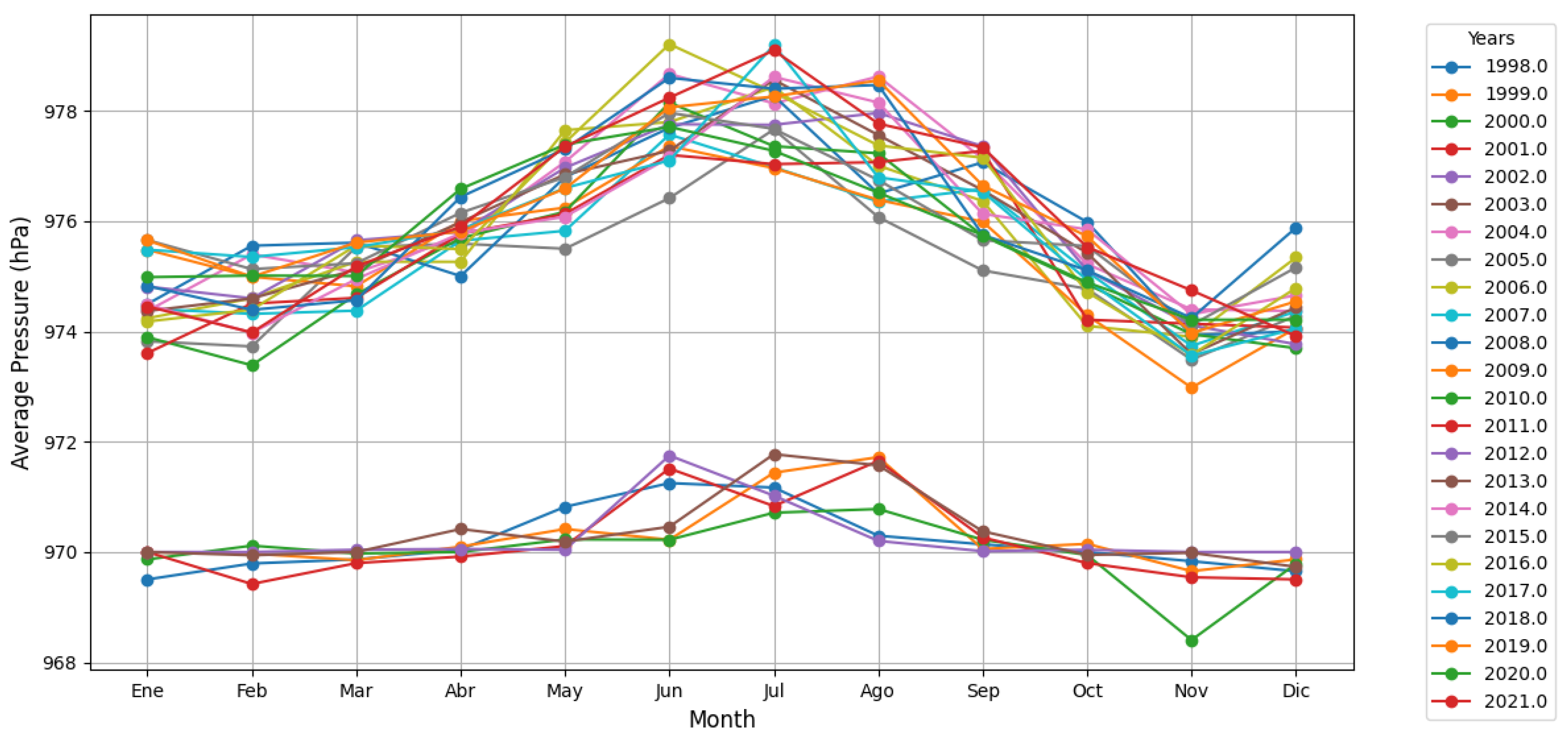
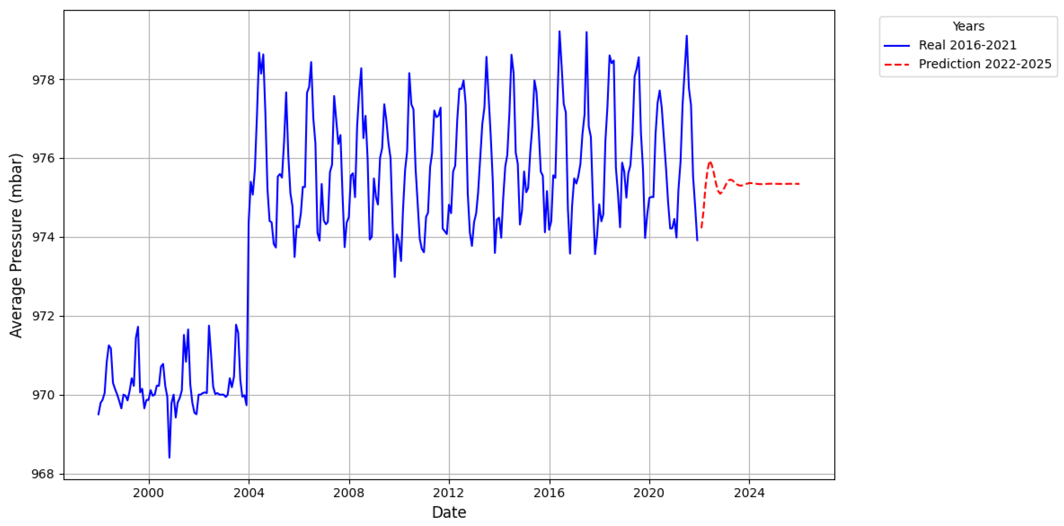
With regard to temperature, it is observed that El Sacha exhibits higher values than Loreto throughout all analyzed periods. Specifically, during the 2016-2021 period, El Sacha attains a maximum temperature of 24.5 °C, exceeding that recorded in Loreto. Concerning atmospheric pressure, this is likewise higher in El Sacha in comparison to Loreto. During the period spanning 2016 to 2021, El Sacha registers a maximum value of 976.0 mbar, which demonstrates a significant difference in the atmospheric conditions between the two localities (see Table 7).

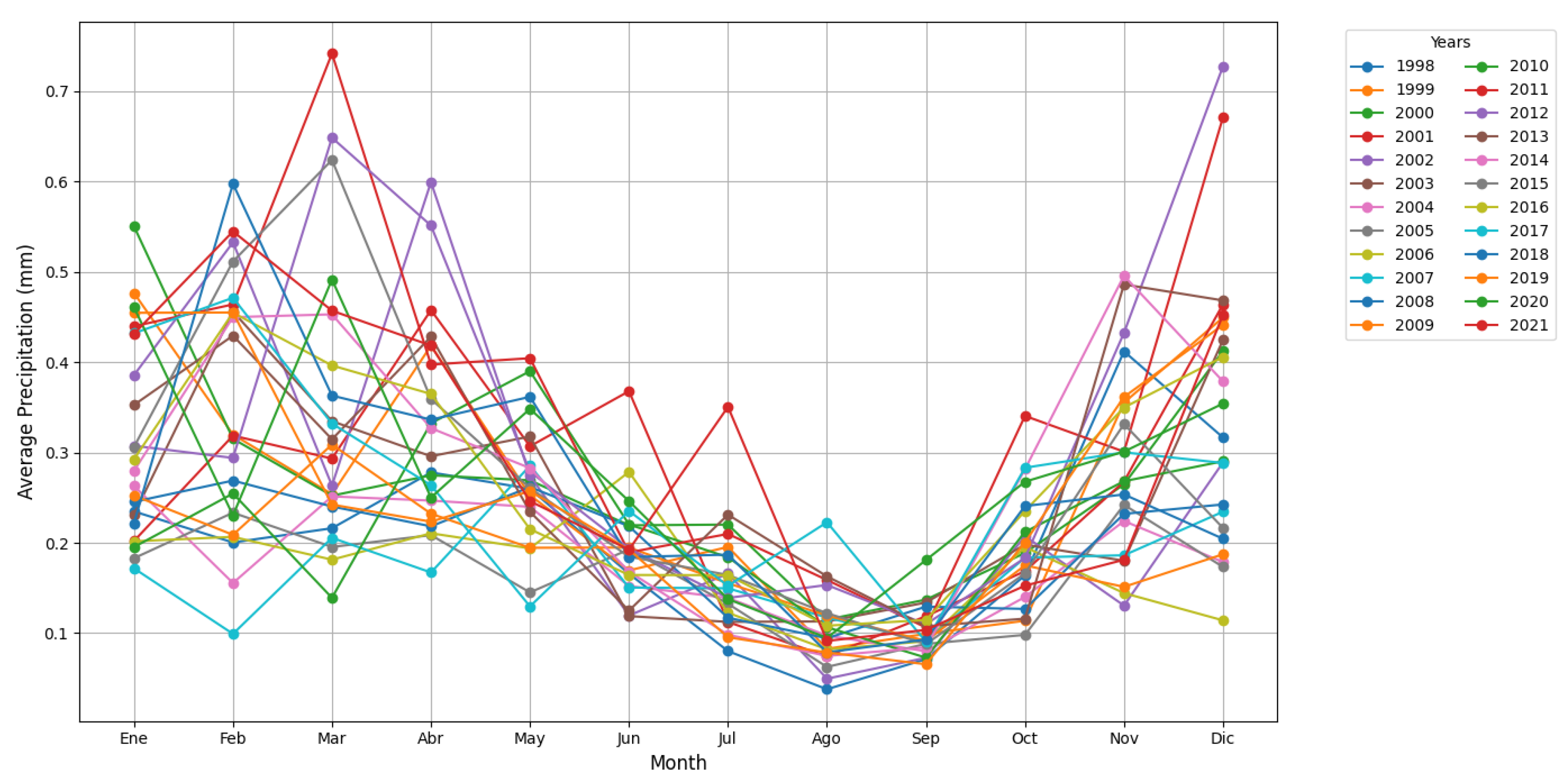
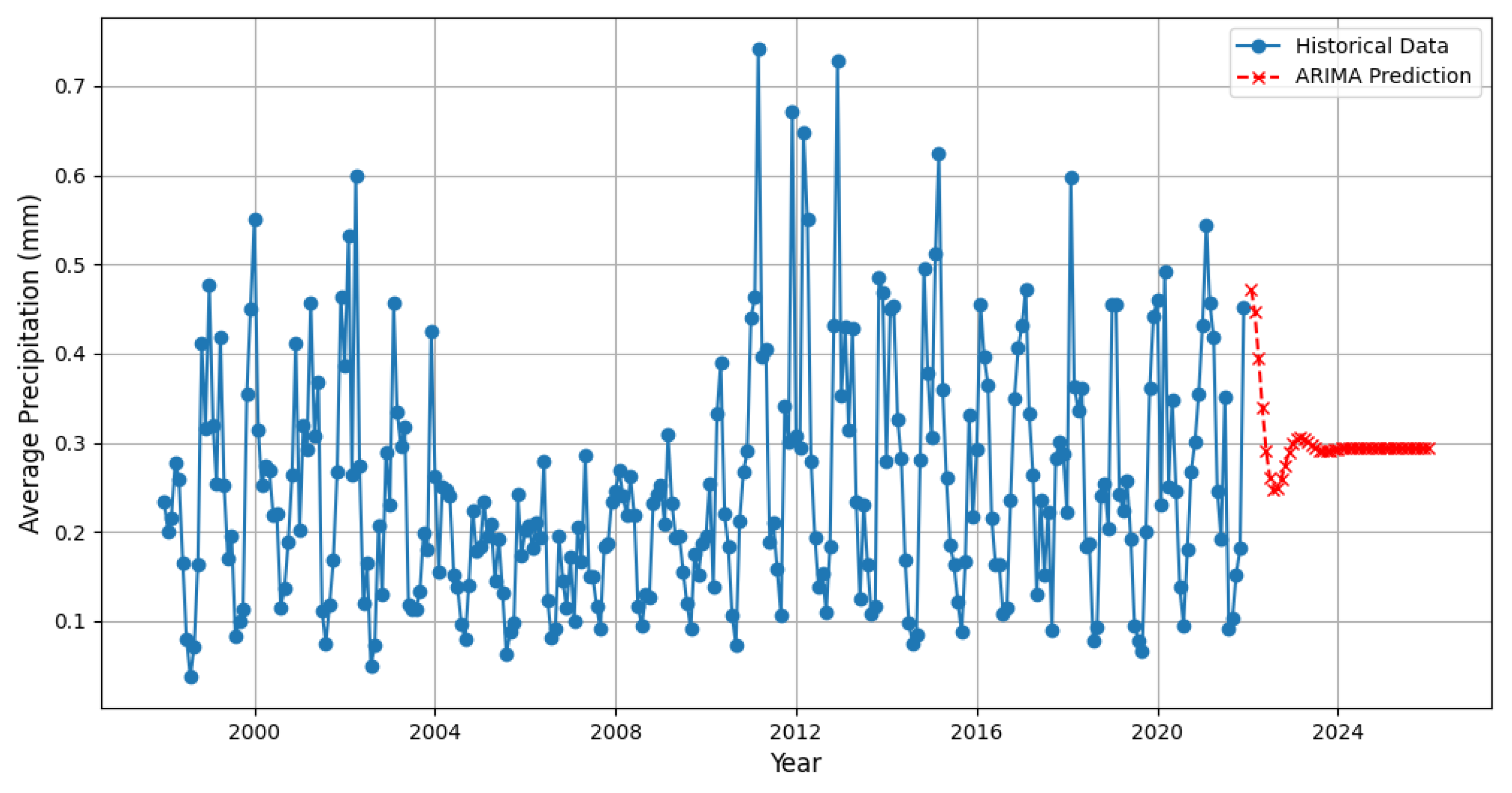
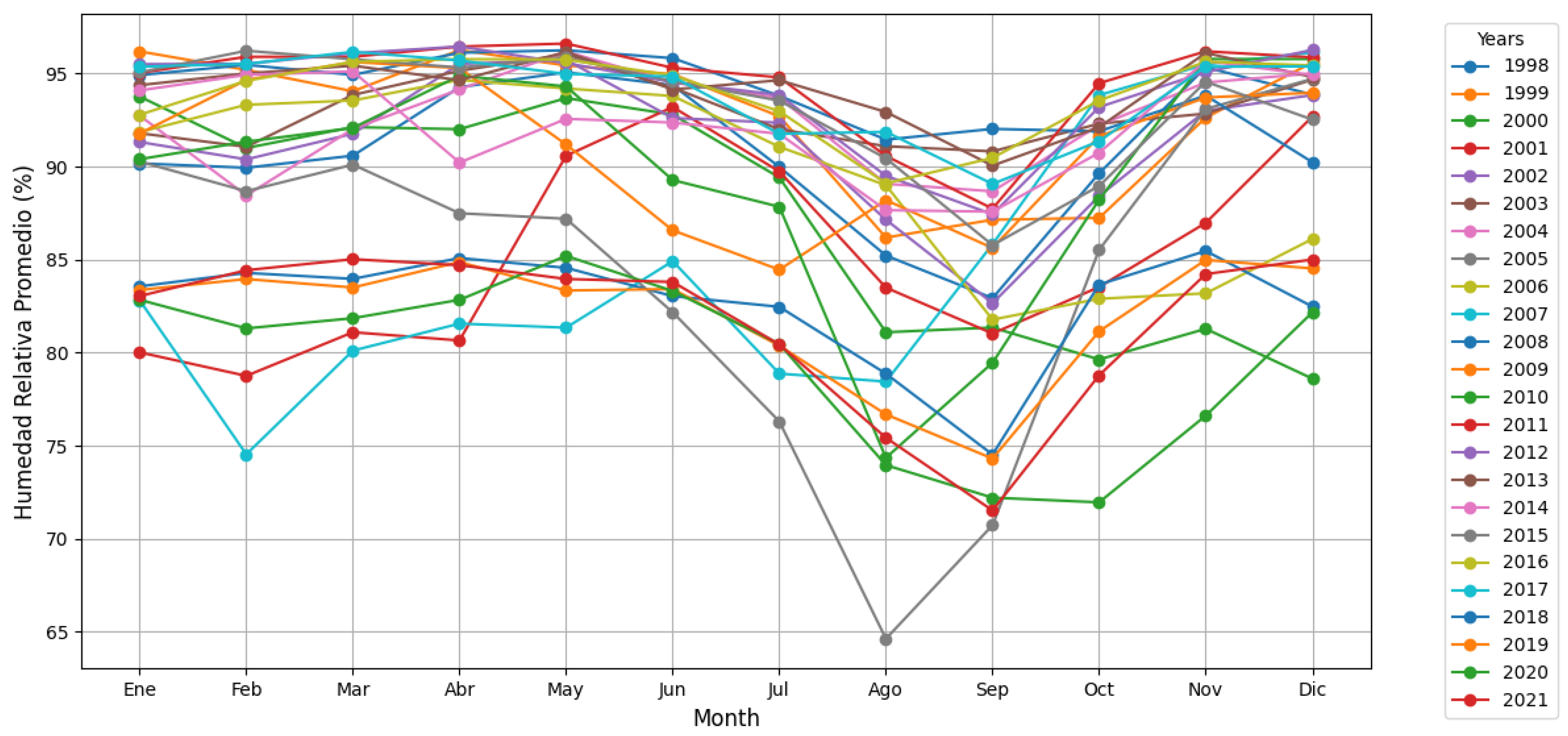
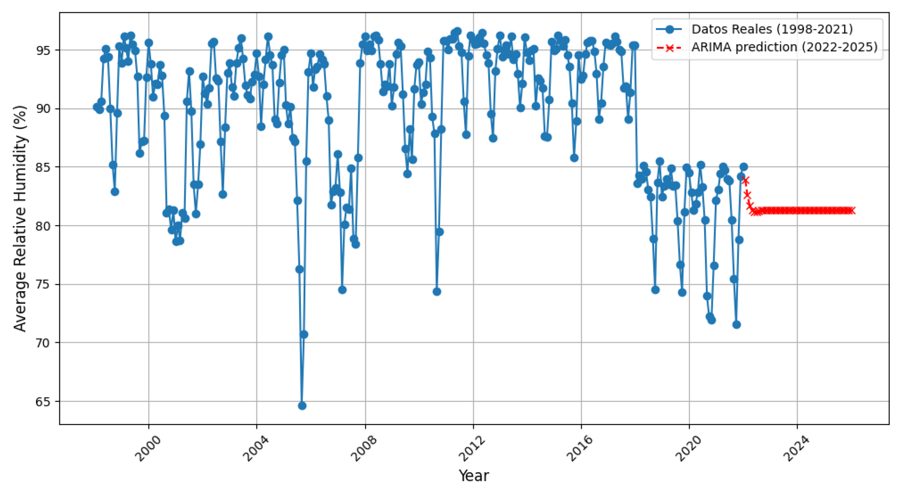
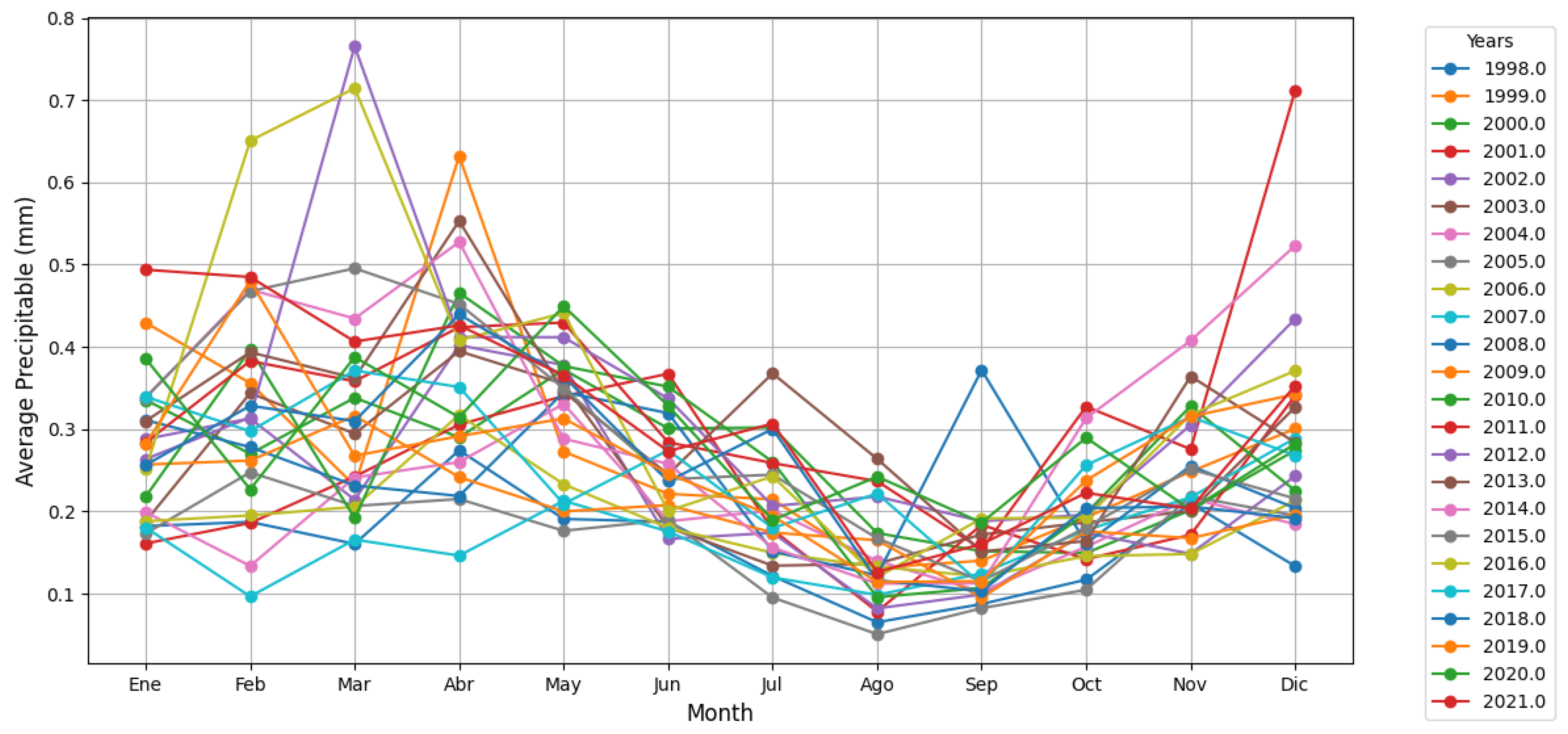
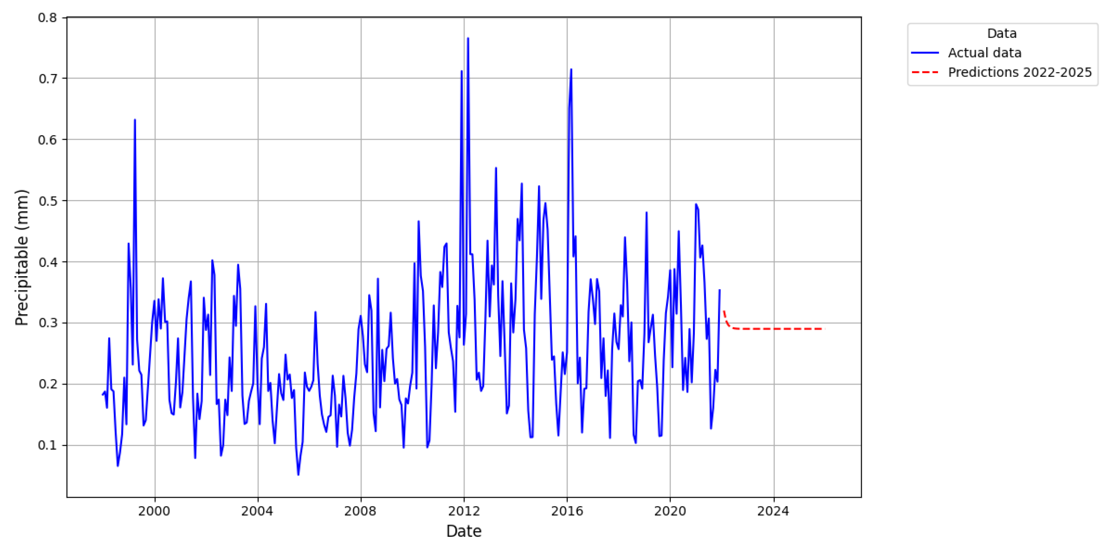
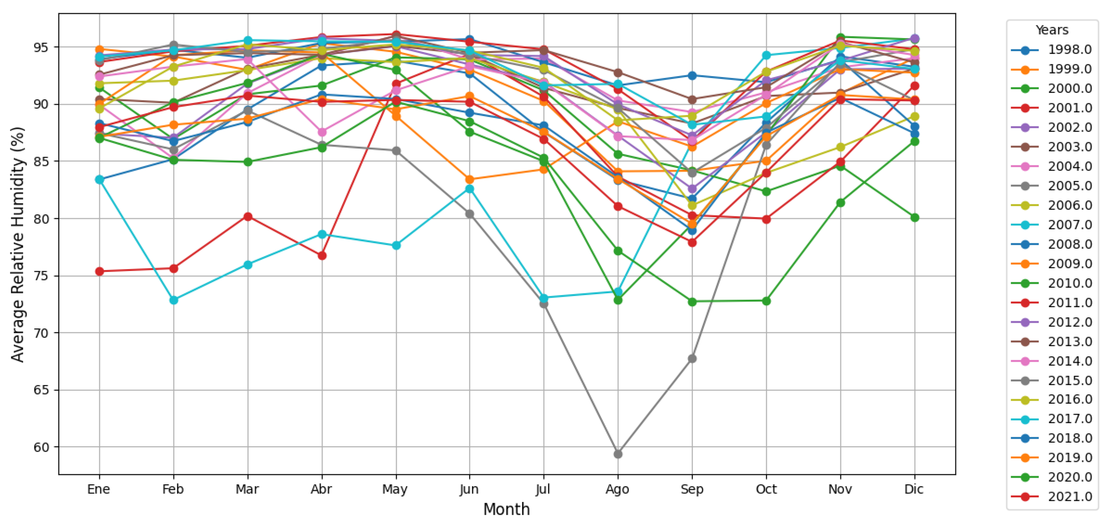
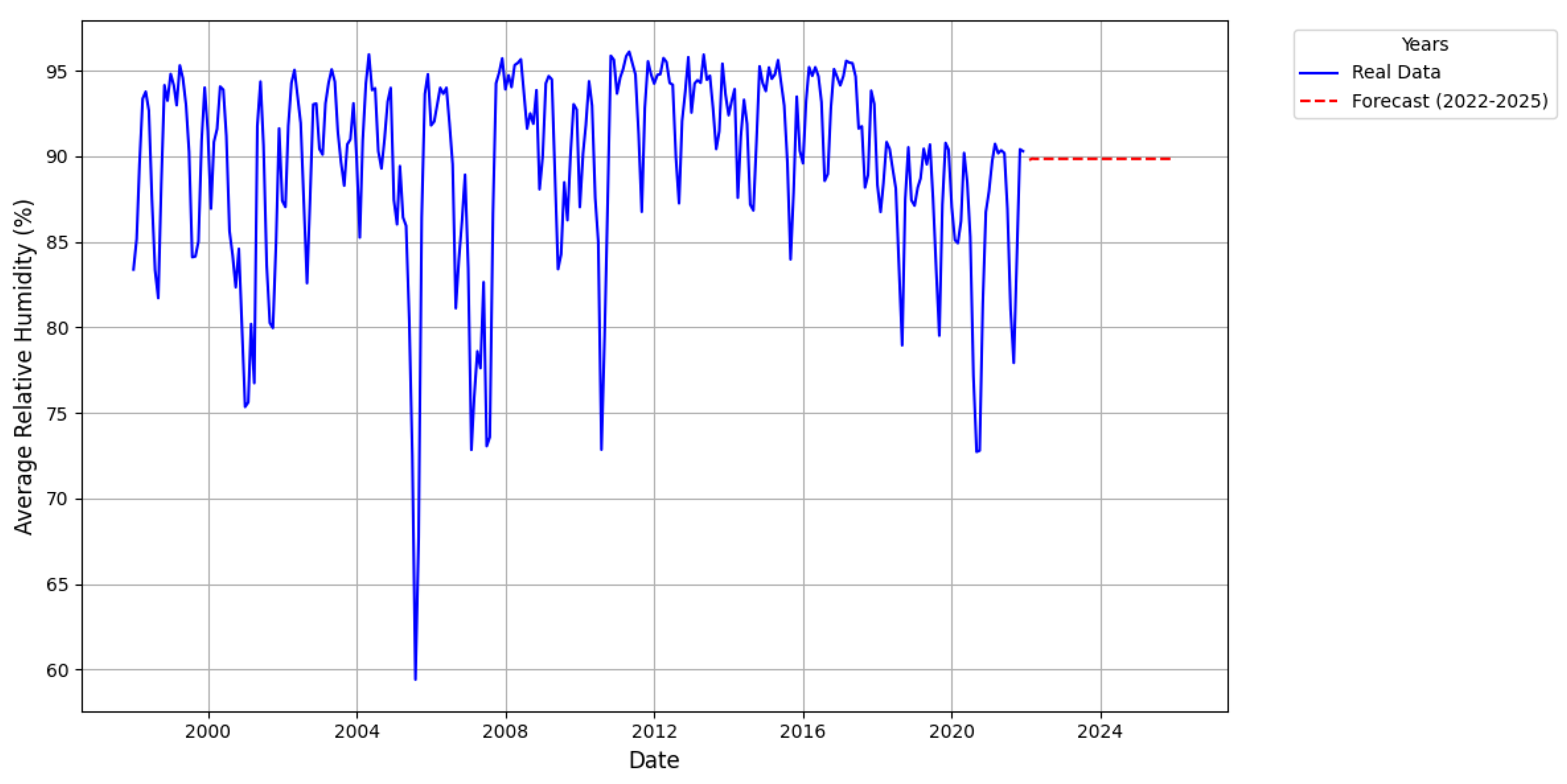
With regard to precipitation, it is observed that El Sacha exhibits a greater quantity of precipitation in comparison to Loreto throughout the majority of the analyzed periods. The period spanning 2010-2015 in El Sacha is particularly noteworthy, registering a value of 0.314 mm. Conversely, relative humidity is significantly elevated in El Sacha relative to Loreto. This phenomenon is particularly pronounced during the 2010-2015 period in El Sacha, with a recorded value of 92.2%. In contrast, Loreto registers its nadir in relative humidity during the 2016-2021 period, with a value of 85.6% (see Table 10).

Table 9. Temperature (°C) and Atmospheric Pressure (mbr)

Interaction effect	Temperature (°C)	Interaction effect	Pressure(mbr)
Loreto (2010-2015)	23.5 ± 1.01 a	Loreto (1998-2003)	930.1 ± 0.88 a
Loreto (1998-2003)	23.7 ± 1.32 b	Loreto (2004-2009)	931.6 ± 1.78 b
El Sacha (2010-2015)	23.8 ± 1.11 b	Loreto (2010-2015)	931.7 ± 1.79 b
El Sacha (1998-2003)	24.0 ± 1.41 c	Loreto (2016-2021)	932.0 ± 1.85 c
Loreto (2016-2021)	24.0 ± 1.10 c	El Sacha (1998-2003)	970.2 ± 1.19 d
Loreto (2004-2009)	24.1 ± 1.42 c	El Sacha (2004-2009)	975.6 ± 1.88 e
El Sacha (2004-2009)	24.3 ± 1.55 d	El Sacha (2010-2015)	975.7 ± 1.88 e
El Sacha (2016-2021)	24.5 ± 1.23 e	El Sacha (2016-2021)	976.0 ± 1.97 f

Table 9. Temperature (°C) and Atmospheric Pressure (mbr)

Interaction effect	Temperature (°C)	Interaction effect	Pressure(mbr)
Loreto (2010-2015)	23.5 ± 1.01 a	Loreto (1998-2003)	930.1 ± 0.88 a
Loreto (1998-2003)	23.7 ± 1.32 b	Loreto (2004-2009)	931.6 ± 1.78 b
El Sacha (2010-2015)	23.8 ± 1.11 b	Loreto (2010-2015)	931.7 ± 1.79 b
El Sacha (1998-2003)	24.0 ± 1.41 c	Loreto (2016-2021)	932.0 ± 1.85 c
Loreto (2016-2021)	24.0 ± 1.10 c	El Sacha (1998-2003)	970.2 ± 1.19 d
Loreto (2004-2009)	24.1 ± 1.42 c	El Sacha (2004-2009)	975.6 ± 1.88 e
El Sacha (2004-2009)	24.3 ± 1.55 d	El Sacha (2010-2015)	975.7 ± 1.88 e
El Sacha (2016-2021)	24.5 ± 1.23 e	El Sacha (2016-2021)	976.0 ± 1.97 f

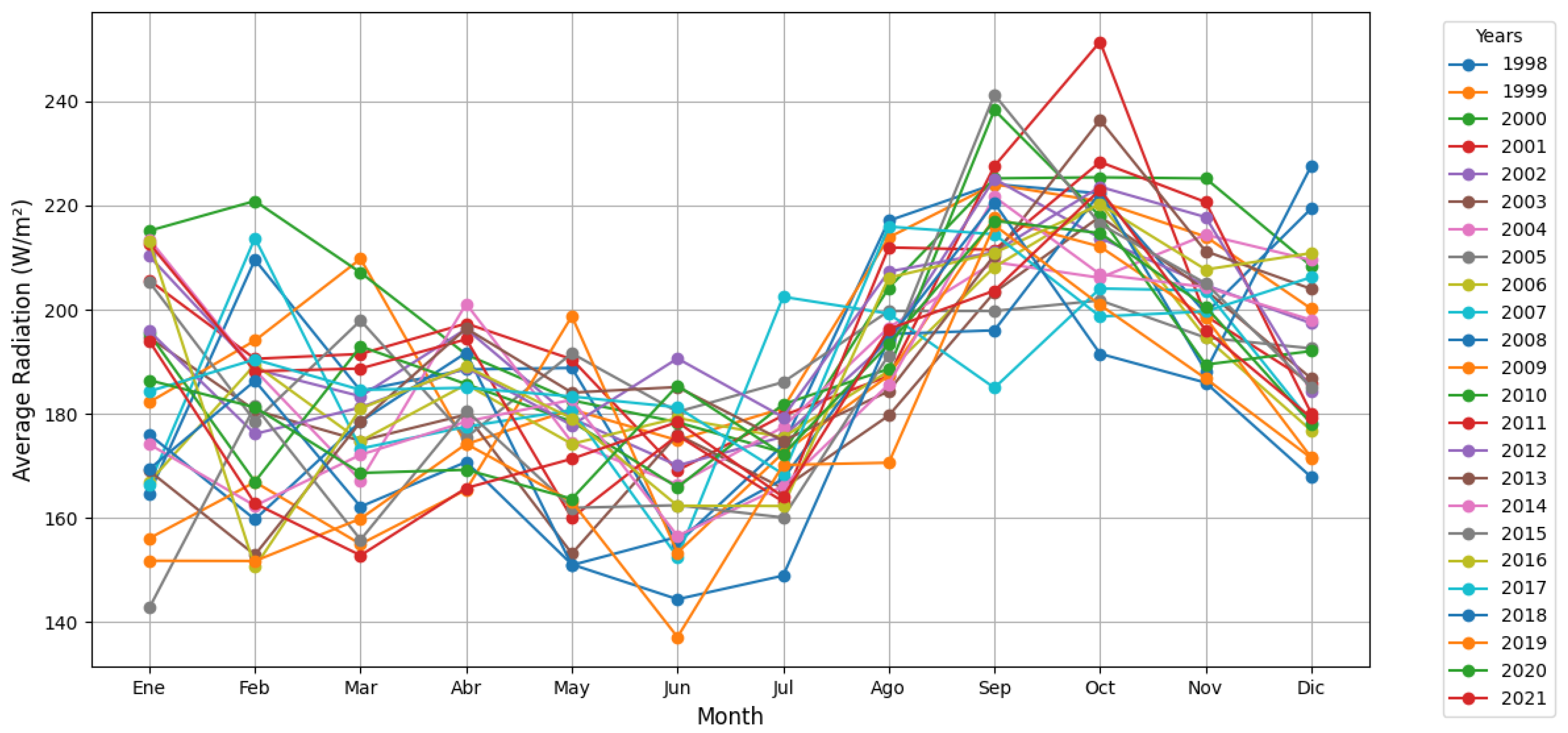
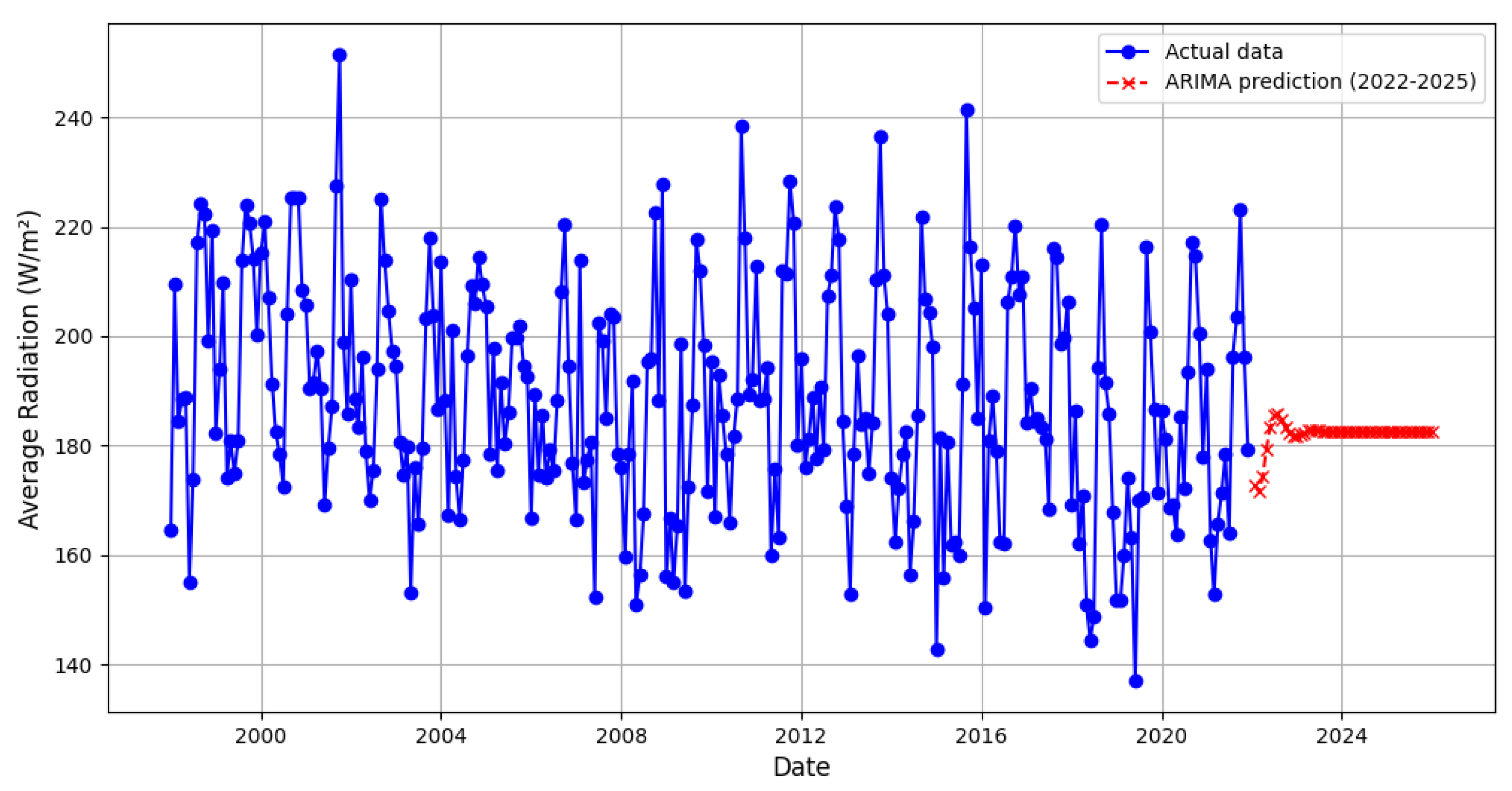
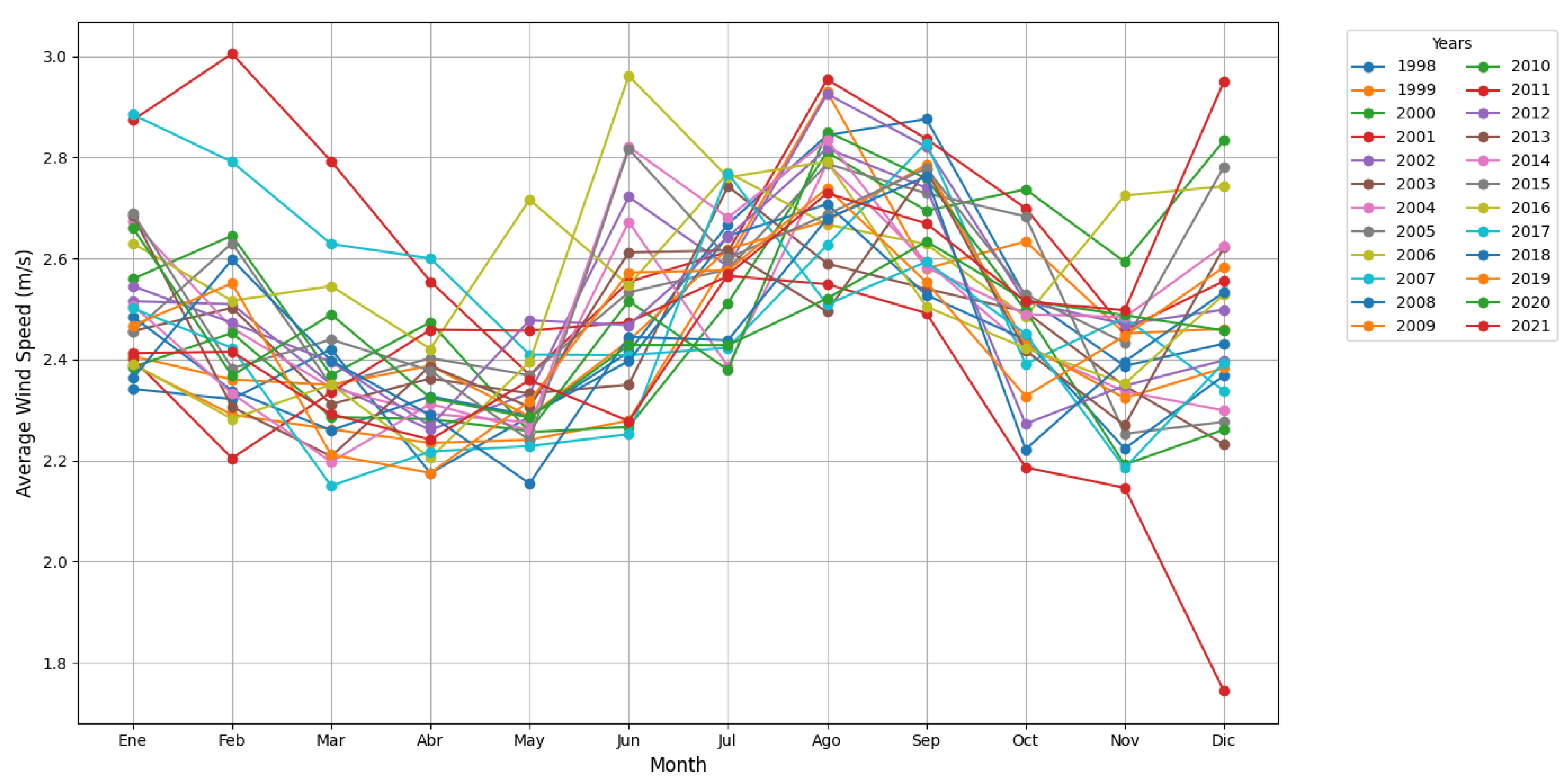
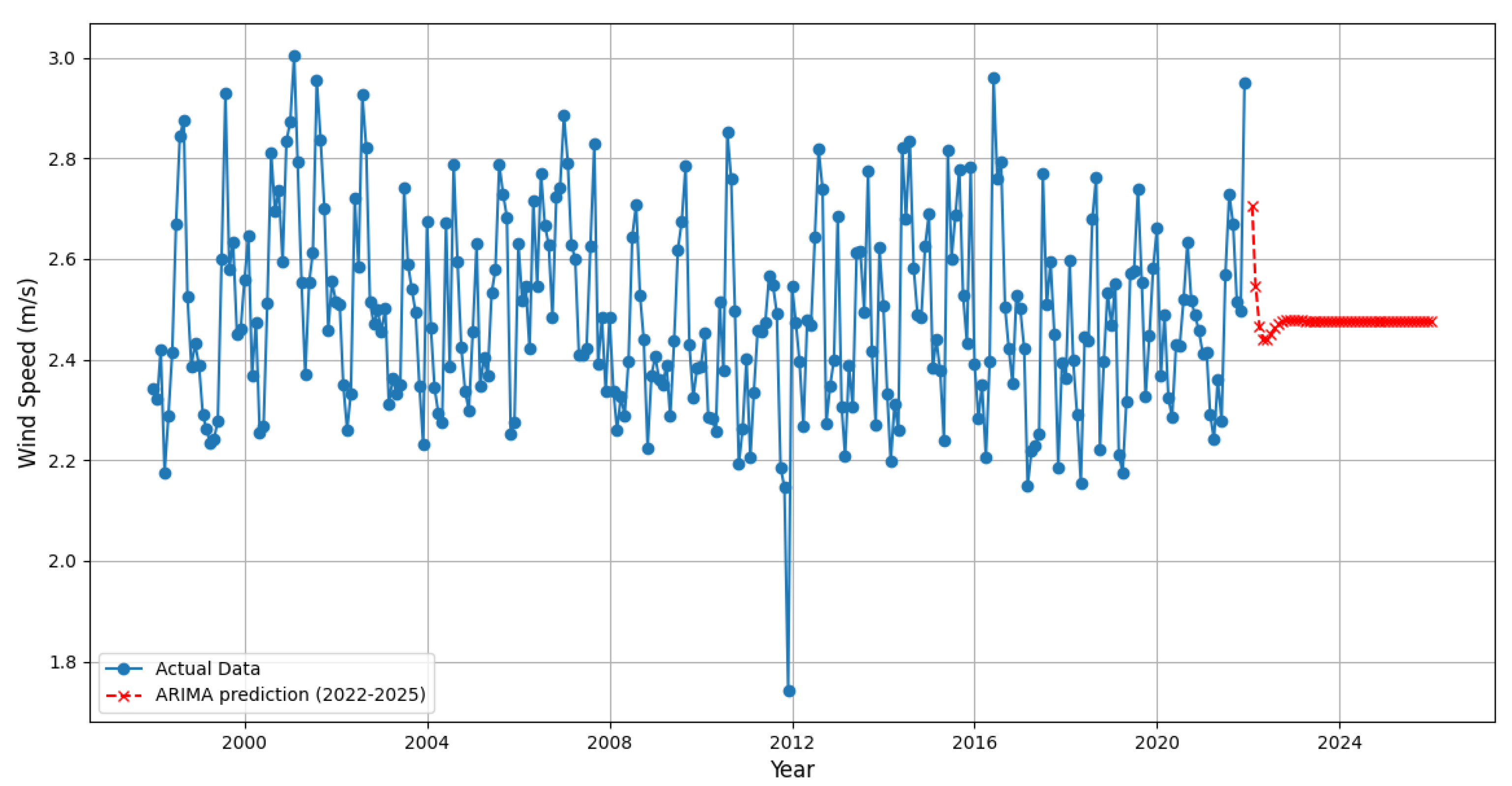
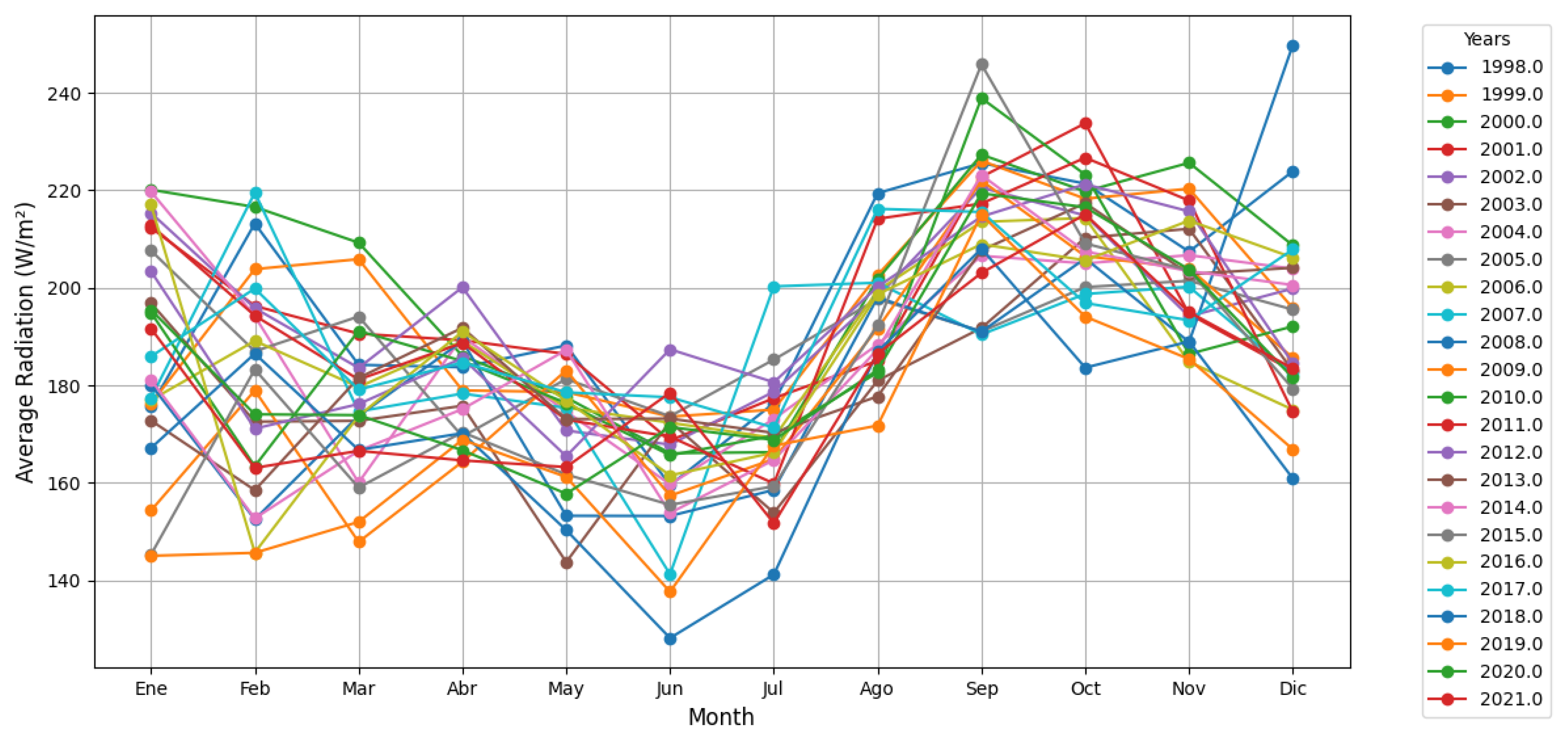
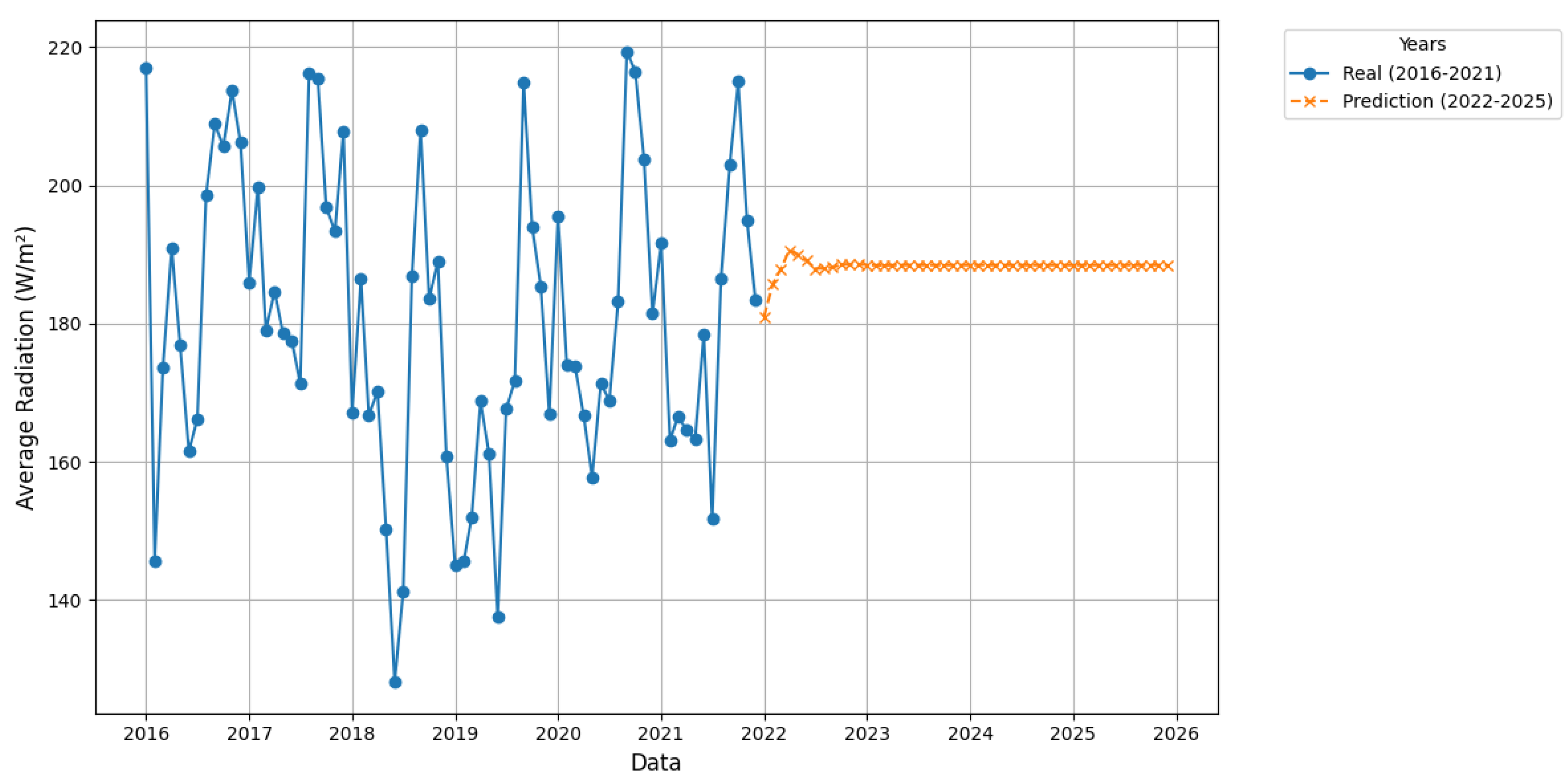
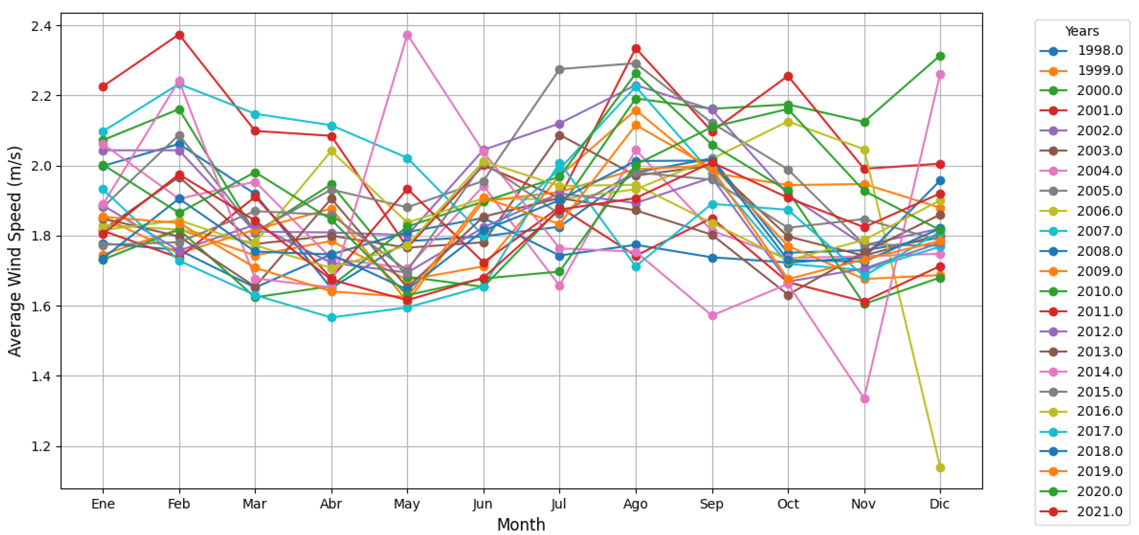
Solar radiation in the Loreto region exhibits elevated levels in comparison to El Sacha, particularly noteworthy between 1998 and 2003, with a mean value of 391.7 W/m². This phenomenon signifies a greater intensity of radiation in Loreto during the aforementioned period. With respect to wind speed, a similar tendency is likewise observed, with higher values recorded in Loreto, reaching up to 2.53 m/s between 1998 and 2003. Conversely, wind speeds in El Sacha are lower, with a maximum of 1.94 m/s within the same temporal interval. These data reflect a significant disparity in the climatic conditions of both zones, which may have implications for renewable energy analyses and other meteorological investigations (see Table 9).

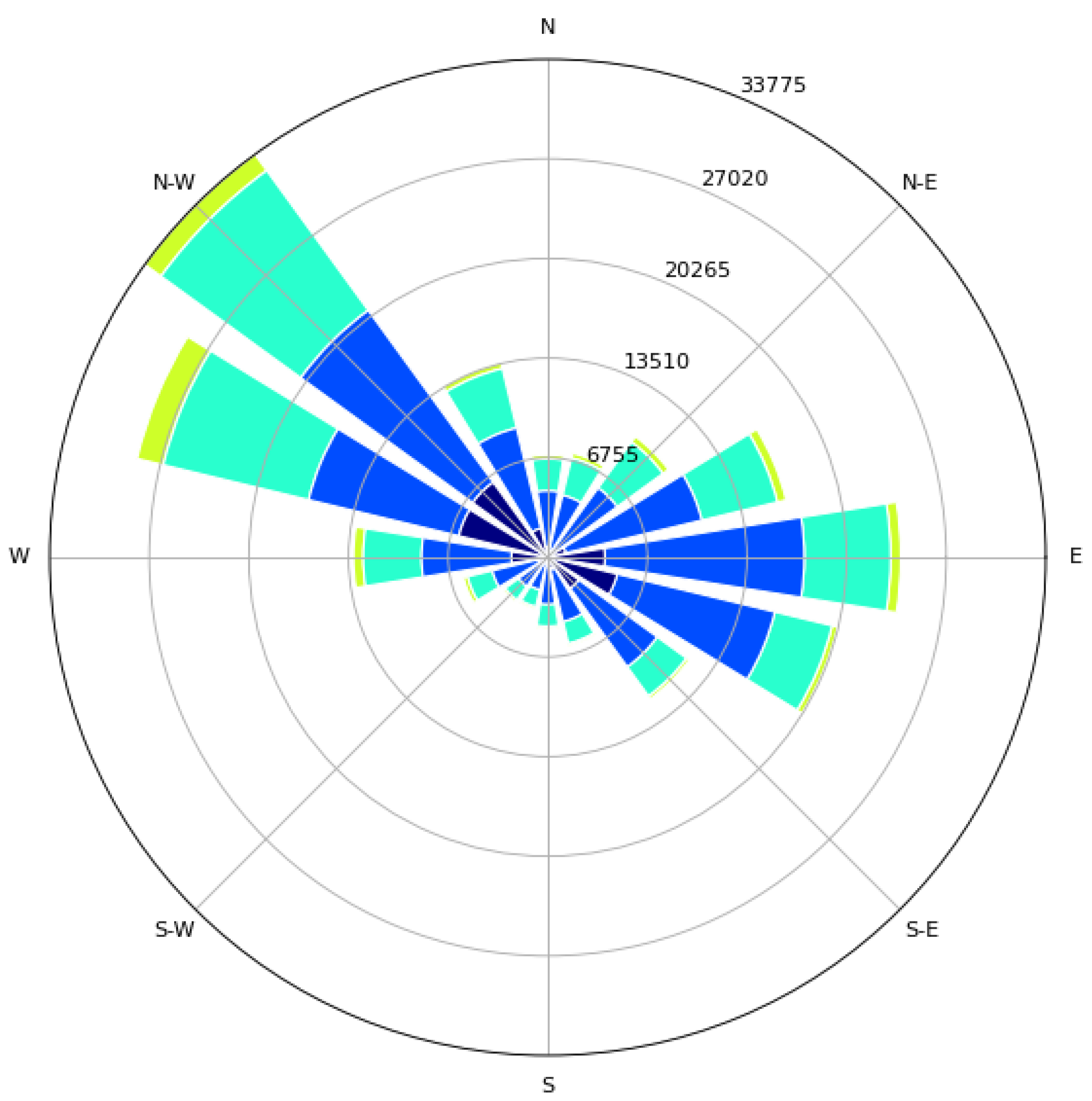
Wind direction exhibits greater variability at the Loreto station, where a range of 200.1° was observed during the period from 2010 to 2015. Conversely, at El Sacha, the wind direction demonstrates greater consistency, with a range fluctuating between 181.9° and 197.2°. This disparity suggests that, whereas Loreto experiences more pronounced fluctuations in wind orientation, El Sacha presents more stable conditions in this respect (see Table 12)

The soil pH in Loreto and Sachas is within the optimal range for the growth of most plant species. However, Loreto exhibits a slightly lower pH value in comparison to Sachas, although both values are conducive to plant development. With respect to NH4 (ammonium) concentrations, both soils are within the optimal range; however, Sachas demonstrates a higher ammonium concentration, which may be advantageous for plant growth, as ammonium serves as a significant nitrogen source.

With regard to phosphorus (P), Loreto demonstrates a deficient level, below the established optimal range, which may potentially limit plant growth in this area. Conversely, Sachas exhibits an adequate value for vegetative development. Potassium (K) concentrations are low in Loreto, which may restrict plant nutrition, whereas Sachas exhibits a higher concentration, albeit still outside the optimal range.

Concerning calcium (Ca) and magnesium (Mg), it is observed that Loreto’s soil possesses an insufficient calcium concentration, which may negatively impact plant health, while Sachas presents a more suitable value. With respect to magnesium, Loreto exhibits a slightly low value, although within the optimal range, whereas Sachas presents adequate concentrations. Furthermore, both soils exhibit low sulfur (S) concentrations, with the deficiency being more pronounced in Loreto, which may influence plant growth if these concentrations persist.

Micronutrient concentrations such as zinc (Zn), copper (Cu), iron (Fe), and manganese (Mn) are generally within optimal ranges in both soils. However, in Loreto, elevated iron and manganese concentrations are observed relative to Sachas, which may have implications for the uptake of these elements by plants. Finally, boron (B) concentrations are low in both samples, which may limit the efficacy of certain metabolic processes in plants.

With regard to organic matter (OM), Sachas is notable for possessing a significantly higher concentration compared to Loreto, which indicates a superior nutrient content and enhanced soil fertility (see Table 13)

With respect to the Al + H and Al (Aluminum + Hydrogen and Aluminum) parameters, both values are within the appropriate ranges for the soils under investigation, suggesting an optimal equilibrium of acidity and toxicity in both instances.

Conversely, the relationship between Ca/Mg, Mg/K, and (Ca+Mg)/K exhibits significant disparities between the Sachas and Loreto soils. The Sachas soil demonstrates a more balanced calcium-to-magnesium ratio, which is conducive to its stability. In contrast, in the Loreto soil, this ratio is less balanced, which could engender a less propitious environment for plant development.

Finally, upon analysis of the Exchangeable Bases, Sand, Silt, Clay fractions, and the soil texture classification, it is observed that the Loreto soil possesses a higher clay content, thus classifying it as a heavier soil. Conversely, the Sachas soil exhibits a greater silt content, indicative of a lighter texture, which consequently enhances aeration and water drainage, fundamental characteristics for optimal soil health (see Table 14).

The parameters of samples N9FL1, N10FL2, and N11FL3 fall within the permissible ranges for the majority of analyzed elements, including pH, electrical conductivity (EC), and nitrites. Nevertheless, certain exceptions have been identified, notably in the values corresponding to lead and fluoride, which do not attain the optimal levels stipulated according to quality criteria. This finding indicates the necessity of a more comprehensive review of these parameters to ensure conformity with environmental standards.

The values of pH, electrical conductivity (EC), and other key parameters are typically observed to fall within the permissible ranges stipulated by water quality regulations, indicating that the majority of water samples meet the minimum safety and health requirements for human consumption and other applications. These parameters are essential for assessing water suitability in terms of its acidity or alkalinity, electrical conductivity (which reflects the concentration of dissolved ionic species), as well as other factors that exert a direct impact on public health and industrial processes.

Notwithstanding this, certain samples exhibit elevated concentrations of lead and fluoride, which do not conform to the standards prescribed by quality regulations. Lead, even at low concentrations, can elicit significant toxic effects on human health, particularly in children and pregnant women, by impairing neurological development and inducing neurological disorders. Concurrently, fluoride, while demonstrating beneficial effects at low concentrations for dental health, can prove detrimental when present at elevated levels, predisposing individuals to conditions such as dental and skeletal fluorosis. These non-permissible values constitute a cause for concern, underscoring the necessity for continuous monitoring and, potentially, the implementation of remedial measures to mitigate these contaminants to safe concentrations.

The results derived from the analysis of water samples intended for human consumption and domestic use are essential for evaluating the quality of water available across diverse regions. The presented tables furnish a detailed analysis of the various samples, thereby enabling a clear comprehension of the status of key parameters in relation to the limits stipulated by sanitary and environmental regulations. This analysis not only facilitates the identification of parameters that adhere to established quality standards but also underscores those that fail to attain permissible levels, thus necessitating immediate intervention.

The presence of impermissible constituents, such as lead, fluoride, or other compounds present in excessive concentrations, may engender grave consequences for human health. In this context, protracted exposure to contaminants such as lead can induce damage to vital organs, while excessive fluoride can exert deleterious effects on skeletal and dental health. Consequently, intervention aimed at ameliorating water quality is not merely a technical consideration but rather an urgent imperative to forestall public health exigencies.

This type of exhaustive analysis is of paramount importance in ensuring continuous access to potable and safe water, a resource indispensable for human life and well-being. Furthermore, water quality exerts a direct influence on the prevention of waterborne illnesses, such as diarrheal diseases, which constitute a primary cause of morbidity and mortality in numerous regions globally. The availability of clean and safe water is inextricably linked to public health and quality of life, as it influences hygiene practices, food security, and the overall development of communities.

Likewise, a meticulous analysis contributes to the sustainability of water resources, which is of particular relevance within a context characterized by water scarcity and escalating pollution. Preserving water quality and guaranteeing its equitable distribution are endeavors that necessitate long-term strategic planning and the implementation of robust protection, treatment, and conservation measures (see Table 15).

Moreover, these analyses furnish those responsible for water management and public health with a critical instrument for informed decision-making. Precise information pertaining to water quality facilitates the formulation of appropriate policies, the identification of problematic locales, and the development of action plans for water treatment and purification. This encompasses the enhancement of distribution infrastructures, the adoption of advanced purification technologies, and the education of communities in appropriate water stewardship practices.

The parameters observed in samples N9FL1, N10FL2, and N11FL3 conform to the quality criteria stipulated for water intended for agricultural irrigation. Initially, the values of pH and electrical conductivity (EC), in conjunction with the sulfate concentration, are within the permissible limits defined for agricultural utilization. Moreover, the concentrations of heavy metals, including arsenic, iron, and chromium, are also within acceptable ranges.

These findings indicate that the physicochemical characteristics of the water under consideration are suitable for agricultural use, presenting no risk to crop production. The analyzed results of water samples obtained in Loreto (N9FV1, N10FV2, and N11FV3) reveal that all key water quality parameters comply with the established criteria for their use in agriculture and irrigation, according to international and local regulations.

Regarding pH, all samples remained within the optimal range for agricultural use, established between 6.5 and 8.5. The obtained values were 6.77, 7.14, and 6.65, respectively, which ensures the water’s suitability to guarantee that nutrients are accessible to plants, without risk of toxicity.

In terms of electrical conductivity (EC), which indicates the concentration of soluble salts in the water, the values were 47.63, 19.7, and 33.46, all within the permitted limits. This ensures that the water does not present a high concentration of salts, preventing potential salinity problems that could negatively affect crop growth.

Sulfate levels in the Loreto samples were 45, 54, and 41 mg/L, values significantly below the permissible limit of 250 mg/L. This indicates a low sulfate concentration in the water, which favors nutrient absorption by plants and eliminates the risk of toxicity.

Regarding heavy metals, such as arsenic, iron, chromium, copper, lead, and cadmium, it was observed that all levels remained below the established limits. Arsenic values were 0.016, 0.014, and 0.012 mg/L, well below the permissible limit of 0.1 mg/L. Iron levels were 0.24, 0.8, and 0.85 mg/L, all within the permitted limit of 5 mg/L. Furthermore, no levels of cadmium or lead were detected in the samples, which confirms the absence of risks associated with these toxic metals. Regarding chromium and copper, the values were 0.023, 0.04, and 0.5 for chromium, and 0.12, 0.18, and 0.18 for copper, which remained within acceptable levels, supporting the water’s safety in relation to heavy metals.

Finally, nitrite levels, which can be harmful in high concentrations, remained at low values. Nitrite concentrations were 0.1, 0.052, and 0.005 mg/L, all below the permissible limit of 0.5 mg/L, eliminating any risk of nitrite toxicity in the water intended for irrigation (see Table 16).

The results presented in the table indicate that all water parameters for irrigation in the Sacha sample conform to the permissible levels stipulated by the established quality criteria. Nonetheless, certain exceptions were identified wherein the values of some parameters approach the upper threshold of the permitted standards. Specifically, the pH in sample C11FL3 exhibited a value of 9.05, while the electrical conductivity (EC) in the same sample registered 198. These values, albeit within the established limits, necessitate continuous monitoring, as their exceedance could engender adverse effects on the agricultural utilization of the water, thereby altering the optimal conditions for irrigation.

The results largely adhere to the quality criteria established for agricultural water utilization, as evidenced by the analyzed parameters. The reported values are, in general terms, within the prescribed limits, thereby suggesting that the water may be employed safely for agricultural irrigation without presenting an immediate hazard to crops or soil. This finding is of considerable importance in regions where water quality may undergo significant variations due to factors of either natural or anthropogenic origin.

Notwithstanding, a singular instance was identified in sample C11FP3, wherein the copper content attained a value of 13, substantially exceeding the permissible limit of 0.2 stipulated by current regulatory frameworks. This elevated concentration constitutes a potential hazard to soil and plant health, inasmuch as excessive copper concentrations may engender toxicity in crops, negatively impact edaphic biodiversity, and, in the long term, alter the physicochemical properties of agricultural soil. Furthermore, the bioaccumulation of this metal could potentially culminate in adverse effects within the food chain should appropriate control measures not be implemented (see Table 17).

In this context, it is deemed a priority to institute more detailed and periodic monitoring of the copper concentration in irrigation water within this specific area. Furthermore, it would be pertinent to investigate the potential sources of contamination, which may encompass proximate industrial activities, the utilization of pesticides or fertilizers with elevated copper content, or even natural contributions originating from the soil or subsoil. Should the need arise, remedial measures, such as filtration systems or chemical treatments, could be implemented to mitigate copper concentrations within the water prior to its utilization in agricultural activities. These actions would serve to ensure the sustainability of agricultural practices and the preservation of ecosystem health in its entirety (see Table 18).

4. Discussion

The results obtained show significant differences between the localities of El Sacha and Loreto regarding climatic parameters, soil quality, and water. These variations have the potential to significantly influence ecological dynamics, agricultural activities, and public health conditions in both regions.

Regarding climatic conditions, it was observed that El Sacha registers higher temperatures and atmospheric pressures compared to Loreto. This can be attributed to factors such as geographic location, altitude, and specific microclimatic characteristics, which directly affect solar radiation, temperatures, and atmospheric pressure conditions. In particular, the increase in atmospheric pressure suggests a more enclosed environment, possibly associated with local wind and humidity patterns. These findings coincide with previous studies that have highlighted the influence of geographic factors on the regional climate([33])

In contrast, Loreto is characterized by higher solar radiation and higher wind speeds. These conditions, along with lower atmospheric pressure, point to a more dynamic meteorological environment. This scenario is favorable for the development of renewable energies, especially solar and wind sources, which represent strategic opportunities for energy diversification in the region. Furthermore, although El Sacha presents lower wind speeds, its directional stability could be exploited for small-scale renewable energy projects, such as passive ventilation systems or low-power wind turbines([34])

Regarding soil quality, the data reveal that El Sacha has greater fertility due to higher concentrations of organic matter and essential nutrients, such as potassium, calcium, and phosphorus. These factors favor agricultural development, particularly for crops with high nutritional demands. The soil texture, with a higher silt content, also contributes to better aeration and drainage, which is crucial for soil health and plant growth([35])

On the other hand, Loreto’s soils present greater agricultural limitations, derived from a higher clay content and reduced levels of key nutrients such as phosphorus and potassium. Although the high proportion of clay improves water retention, it can also hinder drainage and limit nutrient availability, which poses challenges for agricultural productivity. These observations are consistent with research conducted in other tropical regions, where clay soils require specific management strategies, such as the addition of organic amendments and balanced fertilizers([36])

Furthermore, concerning micronutrients such as boron and sulfur, worrying deficits were identified in both locations. These elements are essential for fundamental metabolic processes in plants, such as protein synthesis and the formation of cell structures. Prolonged deficiency of these nutrients could significantly compromise the yield of staple crops. Therefore, it is recommended to implement sustainable management programs that include regular soil monitoring and specific nutrient supplementation according to crop needs([37])

In Loreto and Sacha, a common seasonal pattern is observed, with higher temperatures at the beginning and end of the year and lower temperatures in the middle. However, predictions indicate that these fluctuations will be less pronounced, suggesting a reduction in future climate variability compared to historical data. This behavior could reflect a stabilization of temperatures in the region during the projected years (2022-2025). In Loreto, a temperature increase is predicted for August and a decrease for June and July, remaining within the historical range without extreme values. In Sacha, on the other hand, projected temperatures are slightly higher than the historical average, but without reaching the extreme peaks of previous years.

Regarding atmospheric pressure, in Loreto it remains almost constant at 932 hPa, which contrasts with the seasonal variability historically observed. This stability reflects a reduction in atmospheric variability, which could be associated with climate stabilization over time. In Sacha, little variability in pressure is also observed, with a slight downward trend, suggesting near-total stability in atmospheric pressure. This phenomenon could be related to global or regional changes in atmospheric dynamics.

Regarding precipitation, a decrease is projected in both Loreto and Sacha over the coming years, with less seasonal variability. This pattern suggests that the seasonality of rainfall will decrease in the coming years, which could be linked to climate changes affecting precipitation patterns in a more stable way. Although the decrease is gentler in Sacha, both regions agree that the frequency of extreme rainfall events will be lower, and average precipitation will tend to be located in the lower range of historical data.

Relative humidity also shows a slight decrease in Loreto, suggesting that the region will become drier over time, especially towards the later projected years (2023-2025). Seasonal fluctuations are smoothed, indicating less variability between months. In Sacha, the pattern is similar, with a tendency towards a gradual decrease in relative humidity. As in Loreto, seasonal fluctuations are attenuated, which could reflect a reduction in ambient humidity compared to historical patterns.

Regarding solar radiation, both sites show a slight increase in projected radiation for the coming years, with fewer seasonal fluctuations. This could indicate a trend towards a sunnier climate, with less pronounced variations than in the past. However, this smoothing of solar radiation fluctuations could be an indicator of changes in climate patterns affecting cloud cover or direct solar radiation in the regions.

Finally, regarding wind speed, a slight upward trend is projected in both Loreto and Sacha, but with minimal variability. This pattern suggests that wind speed will be more constant during the coming years, with a slight increase, but without drastic changes. The lack of seasonal and annual variability in wind speed could imply stability in atmospheric circulation patterns, with little influence from extreme events or meteorological phenomena that alter wind speed

5. Conclusions

The observed variations in temperature, solar radiation, and wind speed between the localities of El Sacha and Loreto underscore the need to adapt land use and energy exploitation strategies to the specific conditions prevailing in each region. These climatic discrepancies not only affect environmental dynamics but also directly influence the development potential of renewable energies and the sustainable management of natural resources.

Regarding soil quality, El Sacha presents a substantial advantage in terms of fertility and bioavailability of essential nutrients for agriculture. These edaphic attributes create a favorable environment for crops with high nutritional requirements, while Loreto faces limitations that require the implementation of specific strategies, such as chemical amendments and sustainable management practices. In this context, the adoption of sustainable agriculture techniques could mitigate the limitations present in Loreto and optimize the area’s agricultural productivity.

On the other hand, the analysis of water quality reveals that, while most samples conform to established standards for irrigation and human consumption, alarming concentrations of lead and fluoride were detected, along with elevated levels of copper in one discrete sample. These chemical anomalies underscore the need for continuous monitoring and the implementation of corrective measures aimed at ensuring environmental safety and public health.

The results obtained in this study are of utmost importance for the formulation and implementation of public policies focused on the sustainable management of resources in both localities. The disparities identified in climatic, edaphic, and hydric parameters emphasize the importance of differentiated approaches that promote environmental sustainability and improve human well-being holistically.

Longitudinal studies are recommended to facilitate a more comprehensive understanding of the underlying causes of the variations detected, particularly regarding water contamination. Furthermore, it would be pertinent to explore the application of innovative technologies in soil recovery and conservation, with the aim of maximizing agricultural potential and ensuring long-term sustainability in both regions.

In both areas, Loreto and Sacha, predictions for the 2022-2025 period indicate a general reduction in seasonal variability and a trend towards more stable conditions. Although a slight trend towards higher temperatures and solar radiation is anticipated, seasonal fluctuations are smoothed, suggesting that the coming years will be less extreme compared to previous periods. Humidity and precipitation also show a gradual decrease, with lower values than those historically observed, while atmospheric pressure and wind speed maintain a relatively constant behavior, with little interannual variability. These changes indicate a transition towards a more stable and less variable climate in both regions, which could have implications for environmental planning and resource management in these areas.

References

1. Hopcroft, P.O.; Valdes, P.J.; Calvin, K.; Bond-Lamberty, B.; Boers, N.; Ghil, M.; Stocker, T.F. Theoretical and paleoclimatic evidence for abrupt transitions in the Earth system. Environmental Research Letters 2022, 17, 093006. [Google Scholar] [CrossRef]
2. Adamo, N.; Al-Ansari, N.; Sissakian, V. Review of Climate Change Impacts on Human Environment: Past, Present and Future Projections. Engineering 2021, 13, 605–630. [Google Scholar] [CrossRef]
3. Das, A.K.; Sharma, A. Climate change and the energy sector. Advancement in Oxygenated Fuels for Sustainable Development: Feedstocks and Precursors for Catalysts Synthesis 2023, pp. 1–6. [CrossRef]
4. Huang, M.T.; Zhai, P.M. Achieving Paris Agreement temperature goals requires carbon neutrality by middle century with far-reaching transitions in the whole society. Advances in Climate Change Research 2021, 12, 281–286. [Google Scholar] [CrossRef]
5. Li, M.; Wu, P.; Sexton, D.M.; Ma, Z. Potential shifts in climate zones under a future global warming scenario using soil moisture classification. Climate Dynamics 2021, 56, 2071–2092. [Google Scholar] [CrossRef]
6. Yohannes, T.; Yu, J.; Jonah, K.; Oo, K.T.; Muleta, D.; Adem, K.; Geremew, T. A bibliographic review on anthropogenic climate change and drought. Environmental Science & Policy 2024, 160, 103830. [Google Scholar] [CrossRef]
7. Birthal, P.S.; Hazrana, J.; Negi, D.S.; Pandey, G. Benefits of irrigation against heat stress in agriculture: Evidence from wheat crop in India. Agricultural Water Management 2021, 255, 106950. [Google Scholar] [CrossRef]
8. Shi, X.; Chen, J.; Gu, L.; Xu, C.Y.; Chen, H.; Zhang, L. Impacts and socioeconomic exposures of global extreme precipitation events in 1.5 and 2.0 °C warmer climates. Science of The Total Environment 2021, 766, 142665. [Google Scholar] [CrossRef]
9. Sinha, A. ..; Chaubey, K.K..; Hariharan, S..; Dayal, D..; Bachheti, R.K..; Bachheti, A..; Pramanik, A.; Sinha, A.; Kumar Chaubey, K.; Hariharan, S.; et al. Second-Generation Bio-Fuels: Strategies for Employing Degraded Land for Climate Change Mitigation Meeting United Nation-Sustainable Development Goals. Sustainability 2023, Vol. 15, Page 7578 2023, 15, 7578. [Google Scholar] [CrossRef]
10. Roy, P.; Pal, S.C.; Chakrabortty, R.; Saha, A.; Chowdhuri, I. RETRACTED: A systematic review on climate change and geo-environmental factors induced land degradation: Processes, policy-practice gap and its management strategies. Geological Journal 2023, 58, 3487–3514. [Google Scholar] [CrossRef]
11. Thanigaivel, S.; Vickram, S.; Dey, N.; Jeyanthi, P.; Subbaiya, R.; Kim, W.; Govarthanan, M.; Karmegam, N. Ecological disturbances and abundance of anthropogenic pollutants in the aquatic ecosystem: Critical review of impact assessment on the aquatic animals. Chemosphere 2023, 313, 137475. [Google Scholar] [CrossRef]
12. Muluneh, M.G. Impact of climate change on biodiversity and food security: a global perspective—a review article. Agriculture & Food Security 2021 10:1 2021, 10, 1–25. [Google Scholar] [CrossRef]
13. van Vliet, M.T.; Thorslund, J.; Strokal, M.; Hofstra, N.; Flörke, M.; Ehalt Macedo, H.; Nkwasa, A.; Tang, T.; Kaushal, S.S.; Kumar, R.; et al. Global river water quality under climate change and hydroclimatic extremes. Nature Reviews Earth & Environment 2023 4:10 2023, 4, 687–702. [Google Scholar] [CrossRef]
14. Ćurić, M.; Spiridonov, V. Early Development of Meteorology. History of Meteorology 2023, pp. 31–62. [CrossRef]
15. Zhou, L.; Zhang, J.; Lu, T.; Bao, M.; Deng, X.; Hu, X. Pollution patterns and their meteorological analysis all over China. Atmospheric Environment 2021, 246, 118108. [Google Scholar] [CrossRef]
16. Spiridonov, V.; Curic, M. Fundamentals of meteorology. Fundamentals of Meteorology 2020, pp. 1–437. [CrossRef]
17. Parolini, G. Weather, climate, and agriculture: Historical contributions and perspectives from agricultural meteorology. Wiley Interdisciplinary Reviews: Climate Change 2022, 13, e766. [Google Scholar] [CrossRef]
18. Boni, Z.; Bieńkowska, Z.; Chwałczyk, F.; Jancewicz, B.; Marginean, I.; Serrano, P.Y. What is a heat(wave)? An interdisciplinary perspective. Climatic Change 2023, 176, 1–23. [Google Scholar] [CrossRef]
19. Hannachi, A. Patterns Identification and Data Mining in Weather and Climate. Patterns Identification and Data Mining in Weather and Climate 2021. [Google Scholar] [CrossRef]
20. Ribeiro, T.; Orion, N. Educating for a Holistic View of the Earth System: A Review. Geosciences 2021, Vol. 11, Page 485 2021, 11, 485. [Google Scholar] [CrossRef]
21. Skene, K.R. Systems theory, thermodynamics and life: Integrated thinking across ecology, organization and biological evolution. Biosystems 2024, 236, 105123. [Google Scholar] [CrossRef]
22. Lu, Q.B. Critical Review on Radiative Forcing and Climate Models for Global Climate Change since 1970. Atmosphere 2023, 14, 1232. [Google Scholar] [CrossRef]
23. de Castro, R.R. Effect of the fuel composition of syngas on the combustion process in Dual-Fuel engine. HAL Thess 2024. [Google Scholar]
24. Shekhar, M.; Sharma, A.; Pandey, P.; Sharma, A.; Dimri, A. Assessing the past and future dynamics of the Asian summer monsoon: Insights from palaeomonsoon synthesis and CMIP6 data. Global Environmental Change Advances 2024, 2, 100004. [Google Scholar] [CrossRef]
25. Kovacs, E.D.; Kovacs, M.H.; Kovacs, E.D.; Kovacs, M.H. Global Change Drivers Impact on Soil Microbiota: Challenges for Maintaining Soil Ecosystem Services. Vegetation Dynamics, Changing Ecosystems and Human Responsibility 2023. [CrossRef]
26. Chakraborty, S.K. Trophic Interactions and Biogeochemical Cycles in River Ecosystem. <italic>Riverine Ecology Volume 1</italic> <bold>2021</bold>, pp. 167–234. [CrossRef]
27. INEC. Pirámide de población. Censo 2020. Cantón Mejía 2020, 1.1, 3–6.
28. Congopare. CONAGOPARES | Orellana |, 2024.
29. Tapia, M.; Heinemann, D.; Ballari, D.; Zondervan, E. Spatio-temporal characterization of long-term solar resource using spatial functional data analysis: Understanding the variability and complementarity of global horizontal irradiance in Ecuador. Renewable Energy 2022, 189, 1176–1193. [Google Scholar] [CrossRef]
30. Ricciardulli, L.; Howell, B.; Jackson, C.R.; Hawkins, J.; Courtney, J.; Stoffelen, A.; Langlade, S.; Fogarty, C.; Mouche, A.; Blackwell, W.; et al. Remote sensing and analysis of tropical cyclones: Current and emerging satellite sensors. Tropical Cyclone Research and Review 2023, 12, 267–293. [Google Scholar] [CrossRef]
31. Edwards, M.R.; Holloway, T.; Pierce, R.B.; Blank, L.; Broddle, M.; Choi, E.; Duncan, B.N.; Esparza, Á.; Falchetta, G.; Fritz, M.; et al. Satellite Data Applications for Sustainable Energy Transitions. Frontiers in Sustainability 2022, 3, 910924. [Google Scholar] [CrossRef]
32. Azariah, W.; Bimo, F.A.; Lin, C.W.; Cheng, R.G.; Nikaein, N.; Jana, R. A Survey on Open Radio Access Networks: Challenges, Research Directions, and Open Source Approaches. Sensors 2024, Vol. 24, Page 1038 2024, 24, 1038–2208.09125. [Google Scholar] [CrossRef]
33. Zittis, G.; Almazroui, M.; Alpert, P.; Ciais, P.; Cramer, W.; Dahdal, Y.; Fnais, M.; Francis, D.; Hadjinicolaou, P.; Howari, F.; et al. Climate Change and Weather Extremes in the Eastern Mediterranean and Middle East. Reviews of Geophysics 2022, 60, e2021RG000762. [Google Scholar] [CrossRef]
34. Grubb, M.; Drummond, P.; Poncia, A.; McDowall, W.; Popp, D.; Samadi, S.; Penasco, C.; Gillingham, K.T.; Smulders, S.; Glachant, M.; et al. Induced innovation in energy technologies and systems: a review of evidence and potential implications for CO2 mitigation. Environmental Research Letters 2021, 16, 043007. [Google Scholar] [CrossRef]
35. Naorem, A.; Jayaraman, S.; Dang, Y.P.; Dalal, R.C.; Sinha, N.K.; Rao, C.S.; Patra, A.K. Soil Constraints in an Arid Environment—Challenges, Prospects, and Implications. Agronomy 2023, Vol. 13, Page 220 2023, 13, 220. [Google Scholar] [CrossRef]
36. Rastogi, M.; Verma, S.; Kumar, S.; Bharti, S.; Kumar, G.; Azam, K.; Singh, V. Soil Health and Sustainability in the Age of Organic Amendments: A Review. International Journal of Environment and Climate Change 2023, 13, 2088–2102. [Google Scholar] [CrossRef]
37. Dhaliwal, S.S.; Sharma, V.; Shukla, A.K.; Verma, V.; Kaur, M.; Shivay, Y.S.; Nisar, S.; Gaber, A.; Brestic, M.; Barek, V.; et al. Biofortification—A Frontier Novel Approach to Enrich Micronutrients in Field Crops to Encounter the Nutritional Security. Molecules 2022, Vol. 27, Page 1340 2022, 27, 1340. [Google Scholar] [CrossRef]
Figure 1. PRISMA methodology for article selection.
Preprints 148958 g001
Figure 2. Loreto and Sacha sampling location map.
Preprints 148958 g002
Figure 3. Monthly temperature averages 1998 - 2021
Preprints 148958 g003
Figure 4. Actual Temperature from 2016 to 2021 and Prediction for 2022-2025
Preprints 148958 g004
Figure 5. Residuals over time
Preprints 148958 g005
Figure 6. Histogram of Residuals
Preprints 148958 g006
Figure 7. Histogram of Residuals
Preprints 148958 g007
Figure 8. Monthly pressure averages 1998-2003
Preprints 148958 g008
Figure 9. Monthly Atmospheric Pressure Forecasting with ARIMA
Preprints 148958 g009
Figure 10. Average Monthly Precipitation (1998-2021)
Preprints 148958 g010
Figure 11. Precipitation Forecast with ARIMA
Preprints 148958 g011
Figure 12. Average Monthly Relative Humidity (1998-021)
Preprints 148958 g012
Figure 13. Relative Humidity Prediction with ARIMA (1998-2025)
Preprints 148958 g013
Figure 14. Average Monthly Radiation (1998-2021)
Preprints 148958 g014
Figure 15. ARIMA Radiation Prediction (2022-2025)
Preprints 148958 g015
Figure 16. Average Wind Speed per Month (1998-2021)
Preprints 148958 g016
Figure 17. Wind Speed Prediction (2022-2025)
Preprints 148958 g017
Figure 18. Wind Rose (1998-2003)
Preprints 148958 g018
Figure 19. Temperature Trend (1998-2022)
Preprints 148958 g019
Figure 20. Prediction of temperature (2022-2025)
Preprints 148958 g020
Figure 21. Average Pressure (1998-2021)
Preprints 148958 g021
Figure 22. Monthly Atmospheric Pressure Forecast (2022-2025))
Preprints 148958 g022
Figure 23. Average Monthly Precipitable (1998-2021)
Preprints 148958 g023
Figure 24. precipitation prediction (2022-2025)
Preprints 148958 g024
Figure 25. Average Relative Humidity (1998-2021)
Preprints 148958 g025
Figure 26. Average Relative Humidity Prediction (2022-2025)
Preprints 148958 g026
Figure 27. Radiation (1998-2003)
Preprints 148958 g027
Figure 28. Solar Radiation Prediction (2022-2025)
Preprints 148958 g028
Figure 29. Wind Speed (1998-2021)
Preprints 148958 g029
Figure 30. Wind Speed Prediction with ARIMA
Preprints 148958 g030
Figure 31. Average wind direction (1998-2021)
Preprints 148958 g031