
Submitted:
10 February 2025
Posted:
11 February 2025
You are already at the latest version
Abstract
The development of smart grids has led to an increased focus of the transmission and distribution network operators on the Optimal Power Flow (OPF) problem. The solutions identified for an OPF problem are vital to ensure the real-time optimal control and operation of electric networks and can help enhance their efficiency. In this context, the paper proposed an original solution to the OPF problem represented by the optimal voltage control from the electric networks integrating wind farms. Based on a fuzzy inference system (FIS), where the fuzzification process has been improved through the fuzzy K-means clustering, two approaches have been developed, representing novel tools for the OPF analysis. The FIS-based first approach considers the load requested at the PQ-type buses and the powers injected by the wind farms as the fuzzy input variables. Based on the fuzzy inference rules, the FIS determines the suitable tap positions for the power transformers to lead at the minimum active power losses. The second approach (I-FIS), representing an improved variant of FIS, calculates the steady-state regime to determine the power losses based on the suitable tap positions for the power transformers determined with FIS. A real 10-bus network integrating two wind farms has been used to test the two proposed approaches, considering comprehensive characteristic three-day tests to thoroughly highlight the performance under different injection active power profiles of the wind farms. The results obtained have been compared with those of the best methods in the constrained nonlinear mathematical programming used in the OPF analysis, sequential quadratic programming (SQP). The errors calculated throughout the analysis interval between the SQP-based approach, considered as the reference, and the FIS and I-FIS-based approaches were 5.72% and 2.41% for the first day, 1.07% and 1.19% for the second day, and 1.61% and 1.33% for the third day. The impact of the OPF by calculating the efficiency of the electric network revealed the average percentage errors between 0.04% and 0.06% for the FIS-based approach and 0.01% for the I-FIS-based approach.
Keywords:
Electric Networks
; Optimal Power Flow
; Fuzzy Inference System
; Clustering
; Fuzzy K-Means
; Wind Energy
1. Introduction
1.1. Motivation
The transition of electric networks toward the “smart grids” concept has led to a more attention on the optimal power flow problem (OPF) [1]. Power flow calculation is used to analyse power systems' operation conditions and determine the state variables' optimal values to improve (minimise or maximise) one or more objectives (technical, economic, or environmental). It helps identify potential changes in the system's load and generation and can also be used to evaluate the risk assessment and system expansion. The power flow can be determined using control variables following predetermined limitations and developing effective resource planning strategies.
An OPF problem can help the decision maker (DM) improve an objective function constrained by physical, security, and operational constraints. Carpentier proposed the first OPF solution in the 1960s [2,3]. The data collected for this problem, which usually consists of load forecasts and network parameters, are then used to develop a strategy for optimising the function.
Probabilistic OPF is the most common type of OPF. Various numerical techniques, such as Monte Carlo simulation [4], have been used to solve these problems. However, the accuracy of the results is not as good as it could be because of the computational burden involved in the calculations. Linearisation of power flow equations can make the analytical approach to the probabilistic OPF more efficient. Several well-known methods have been tested, such as the first-order second-moment [5] and the cumulant method [6]. The accuracy depends on the uncertainty propagation's linear functions. For instance, if the probability distribution is easier than the transformation of the output variables, then some methods, such as the point estimation method [7], are used to get the properties of this distribution.
Unfortunately, the power output from renewable sources is often affected by uncertainties, such as fuzziness and randomisation. The invariable characteristics of the wind speed and solar irradiance usually cause random uncertainty in a power system. The other factors affecting the system's operating condition are the weather changes and the measurement accuracy [8]. Last but not least, the demand-side options and the longevity of the plants can be integrated into the uncertainty category. Technological developments can also cause them, the availability of renewable resources and the regulation of fuel prices [1]. All these factors can make calculating and evaluating the system's condition difficult.
Researchers have long studied the modelling of power system uncertainties. The volatility of fuel prices and generation capacities and the uncertainty related to load forecasting have become important factors that have prompted a renewed focus on this issue. The fuzzy theory can describe the uncertainties in the data when the information is insufficient to produce appropriate distributions. This approach has been successfully tested for the OPF problem.
1.2. Literature Review
Recent academic research on Optimal Power Flow (OPF) has increasingly focused on addressing uncertainties inherent in power networks, particularly integrating renewable energy sources (RES). These uncertainties stem from RES's intermittent nature and the variability in load demands.
Miranda and Saraiava developed [9] a fuzzy model for the operation of the power system. The model considers the uncertainties in the load and generation uncertainty and handles the system behaviour under known injections. The linear programming procedures based on the dual simplex and Dantzig Wolfe decomposition have optimised power flow. The proposed approach has been tested using a 6-bus system. Gomes et al. detailed in [10] a fuzzy optimal power flow model, which considers the uncertainties related to forecasting power system capacities and fuel prices. The model is based on a multi-parametric linear programming method, which can identify various critical regions in the uncertainty space. The developed models were tested using a 6-bus and IEEE 24 bus/38 branch systems. Sarcheshmah and Seif [11] proposed a method to analyse the uncertainty in the power flow using the fuzzy membership functions. The uncertainty in both generations and loads has been modelled with the help of the triangular and trapezoidal fuzzy membership functions. The method has been then used to find the fuzzy distributions of state variables based on a constrained linear programming optimisation. The technique has been tested with the power flow from the 6-bus and IEEE-30 bus systems. Salhi et al. presented in [12] a mathematical model to solve the multi-objective OPF problem. It considers the uncertainties associated with the different objective functions, such as total generation cost, gas emission, and voltage profile index, and their optimisation after several tests. The model uses a genetic algorithm to determine the system's parameters. The researchers used the Algerian electrical network for the 59-bus test system. Varathan and Belwin developed a novel method in [8] to calculate the distribution network's random fuzzy power flow. The first step in this study is to set up the random models of PV and wind power generation for the first time. The two-fold random simulation has been used to analyse the results of the power flow calculations. The proposed method has been tested in two different test systems (IEEE 33 and 69 bus systems). Zhang et al. [13] introduced a method for calculating the OPF designed to consider the uncertainties related to the availability of renewable resources and the demand-side response. Their study also established some uncertainty models for output and power generation for photovoltaics. One of these is the cloud model theory-based uncertainty model for the demand response. The authors used the IEEE 30-bus system to validate the model's efficacy. Luo et al. [14] used a method for the OPF problem by modelling wind generation uncertainties. The uncertainty propagation framework comprised the evidence theory and extended affine arithmetic. The copula theory then handles the dependence among the variables. The proposed method and model have been tested on the IEEE 30-bus system.
The current methods for studying uncertainty propagation in electric networks have limitations. The data and test networks used in these studies, along with the assumptions made about generation sources and nodal loads, may not be sufficient to instil confidence in using fuzzy models in real applications. This issue could cast doubt on the applicability of these models in actual operating conditions.
This paper's main objective is to develop an efficient OPF calculation method that considers the uncertainties related to renewable energy sources, especially wind farms, and loads associated with PQ-type buses. The original contribution refers to building a practical and robust framework that integrates the correlation between the fuzzy models of the production profiles corresponding to renewable energy sources and load profiles of the PQ-type buses obtained through a fuzzy K-means algorithm-based clustering process in various production scenarios and availability cases of renewable energy sources.
To emphasize the novelty and originality of our proposed approach in Table 1, we present a brief description of the relevant literature, considering the six aspects suggested for the efficient Optimal Power Flow (OPF) calculation method that explicitly incorporates uncertainties associated with renewable energy sources (RES) and load variations at PQ-type buses. The acronyms used to highlight the OPF methodologies in the Table are the following significations: Newton-Raphson - Monte Carlo Simulation (NR-MCS) [4,13], First-Order Second Moment (FOSM) [5], point estimate method (PEM) [7], Particle Swarm Optimisation (PSO) [14,18], Wild Horse Optimizer (WHO) [15], Fuzzy-Firefly Algorithm (FFA) [16], non-dominated sorting genetic algorithm-II (NSGA-II) [19], fuzzy multi-objective optimal power flow (FMOPF) [20], the fuzzy logic system with harmony search algorithm (FHSA) [21,24], Multi-objective random-fuzzy (MORF) [22], Fuzzy Systems with Genetic Algorithm and Particle Swarm Optimisation (FZGAPSO) [23], learning-based sine–cosine algorithm (L-SCA) [25], Memory-Guided Jaya algorithm (MG-JA) [26].
Unlike conventional OPF models, which often assume deterministic inputs, our study introduces a fuzzy-based approach to modelling wind production variability and load demand dynamics. This proposed method offers an original solution to the OPF problem by incorporating fuzzy logic, clustering techniques, and real-world data processing. The framework provides an efficient means of addressing uncertainties in renewable energy sources and load fluctuations, presenting a practical alternative for OPF analysis. The results demonstrate the potential of this approach to enhance the reliability and efficiency of electric networks that integrate wind energy.
1.3. Original Contributions
In this context, the main contribution is designing and developing a Fuzzy Inference System (FIS)-based innovative solution to the OPF problem represented by the optimal voltage control from the electric networks integrating wind farms having the following strengths:
Defining the fuzzy models of the requested active and reactive powers at the PQ-type buses and injected by the wind farms integrated into the electric network considered as the input variables and the tap positions for the power transformers (representing the control variables) and active power losses (signifying the objective of the optimization process) used in an OPF analysis. The fuzzy models of the input and output variables are built using the fuzzy K-means clustering method, which allows for improving the definition of the membership functions associated with the linguistic categories resulting from clustering process.
Design and build the fuzzy inference system using the Mamdani method based on an inference rule database. This system determines the suitable tap positions for the power transformers, leading to the minimum value of the active power losses.
Exploring the potential of an improved variant (I-FIS) that integrates an additional steady-state calculus based on the Newton-Raphson method. Considering the tap positions determined by the FIS-based approach, this exploration proved promising, highlighting the possibility of enhancing the performance of the estimation process associated with power losses.
Evaluating the impact of the OPF on the efficiency of the electric network.
To test the Fuzzy Inference System (FIS)-based innovative solution, a real 10-bus network integrating two wind farms, representing a zone from the Romanian power system, has been used. The results obtained from the FIS and I-FIS-based approaches have been compared with those of the best methods in the mathematical programming category, the SQP-based approach demonstrating a high performance what they recommend in their practical implementation with economic and technical benefits for the ENOs.
1.4. Paper Structure
In the following, the structure of the paper has three sections. Section 2 presents details regarding the OPF problem in the electric networks integrating wind energy. Section 3 integrates Fuzzy Inference System-based approach in the OPF analysis. Section 4 includes the case study with the obtained results and discussions. Section 5 contains the discussions, conclusions and the future work.
2. OPF Problem in Electric Networks Integrating Wind Energy
2.1. OPF Problem in Electric Networks
Various approaches regarding the system modelling and optimization methods have been proposed to solve the OPF problem in electric networks integrating renewable sources (among which wind energy sources), see Figure 1 [27].
Most of these were not tested on actual electric networks. Instead, they have been implemented in electric networks integrating renewable energy sources. The performance of classical mathematical methods has been compared in many studies with meta-heuristic algorithms. The computation time and number of iterations used in the comparison revealed that mathematical programming-based methods perform better than the meta-heuristic algorithms. Thus, if the IEEE-30 bus standard is used as the reference, the meta-heuristics algorithms determine the solutions in several iterations in hundreds of seconds. The computational time for these algorithms ranged from around 5 to 12 minutes, while in the case of classical algorithms, it is of the order of seconds. In this case, classical algorithms can be a better solution [28,29]. They can solve the issue in real time and integrate wind farms into electric networks.
2.2. OPF Formulation
The formulation of an OPF problem starts from the general optimization model:
where: X – the vector of the optimization variables regarding the bus voltages expressed through the magnitude and angle when the polar coordinates are used or the real and imaginary components when the Cartesian coordinates are used, the branch power flows, generated active and reactive powers of the power plants; n – the number of the buses from the electric networks; Y – control variables concerning to the generated active power of the power plants (classical and wind farms), voltage magnitudes of the generation bus (PU-type bus), tap positions of the power transformers, load shedding, reactive powers of the Static Synchronous Compensator (STATCOM) devices; gi(X, Y) – the equality equations associated with the active and reactive power balances at each bus of the electric network; hl – the inequality constraints including the minimum and maximum operating limits of the voltage magnitudes, branch power flows, generated active and reactive power of the power plants, tap settings of the power transformers; ne – the number of the equality constraints; ni – the number of the inequality constraints.
2.2.1. Objective Function
2.2.2. Technical Constraints
- Equality restrictions
The balances of the active and reactive powers
- Inequality restrictions
Voltagemagnitude
The injected powers of the classical power plants
The injected powers by the wind farms
Transformer tap
Line loading
where: Ns – the slack bus representing the link with the power system of the analysed EN; NPU – the generator buses’ set; , - the real and imaginary parts calculated for the component c between the buses bi and bo;, – the hourly injected active and reactive powers at the level of bus bi, in [MW] and [MVAr], respectively; , – the required active and reactive powers at the level of bus bi, in [MW] and [MVAr], respectively; , – the hourly injected active and reactive powers corresponding to the classical power plant CPP, in [MW] and [MVAr], respectively;, - the extreme limits (minimum and maximum values) corresponding to the injected active power of the classical power plant CPP, in [MW]; , - the extreme limits (minimum and maximum values) corresponding to the injected reactive power of the classical power plant CPP, in [MVAr]; – the hourly injected active power of the wind farm WF, in [MW]; , - the extreme limits (minimum and maximum values) corresponding to the injected active power of the wind farm WF, in [MW]; – the tap position of the On-Load Tap Changer (OLTC) associated with the power transformer connected between buses bi and bo at the hour h, h = 1, …, NH; , - the minimum tap below median tap of the OLTC; - the maximum tap above median tap of the OLTC; - the hourly apparent power flow in the electric line connected between buses bi and bo, in [MVA]; – the maximum limit corresponding to the apparent power flow in the electric line connected between buses bi and bo, in [MVA].
Finally, the ENOs assess the impact of the OPF by calculating the efficiency of the electric network at each hour h, where h = 1, …, NH, aiming for a value as close to 100% as possible:
where: E(h)EN – the efficiency of the electric network EN at the hour h; P(h)inj,EN – the total hourly injected active power at the level of the electric network from all energy production sources (classical and renewable) and the slack bus (which ensures the link with the external power system); Γ(h)EN – the total hourly power losses from the electric network.
3. Fuzzy Inference System-Based Approach in OPF Analysis
3.1. Fuzzy Sets and Fuzzy Logic
One of the most popular applications of the fuzzy sets theory and fuzzy logic is the development of fuzzy inference systems. These systems can be used for various tasks, such as diagnosis and classification. The main strength of a fuzzy inference system (FIS) lies in its dual identity. On the one hand, it can handle linguistic concepts; on the other hand, it can perform non-linear mappings between outputs and inputs [30].
In the proposed approach, the authors offer a solution to the significant issue of the OPF problem, represented by the tap position of the power transformers. Based on a fuzzy inference system, our solution considers several influential factors associated with the load requested at the PQ-type buses (represented by the active and reactive powers) and the powers injected by the generation sources (classical or based on renewable energy such as wind, solar, biomass, etc.). The load dynamics at the level of PQ-type buses and the intermittent character of renewable energy sources can lead to uncertainties regarding the input data of the OPF analysis. By integrating these uncertainties modelled using fuzzy logic, the proposed system can improve decision-making regarding the tap positions of the power transformers, significantly affecting the operation regimes of the electric networks through the minimisation of power losses.
A fuzzy inference system (FIS) was built to determine suitable tap positions for the power transformers to lead at the minimum active power losses. Figure 2 presents the basic structure of the FIS.
The Mamdani inference method was used instead of the Sugeno and Takagi methods because it is more efficient when using human reasoning and intuition [31].
The fuzzy models were obtained starting from a clustering process. The input data were associated with the active and reactive powers requested at the PQ buses and injected by renewable energy sources (the wind farms in our case study). The clustering process allowed our model to analyse the input data comprehensively and define the membership functions of linguistic categories associated with the obtained clusters. The proposed FIS determines the tap positions of the power transformers and the associated power losses.
3.2. Fuzzy Inference Systems
This section describes the features of the proposed FIS that is based on a rule base with a linguistic variable in its resulting framework, which is known as a linguistic rule.
A linguistic rule is a representation of a domain's knowledge base using the propositions of fuzzy logic. It establishes the relationship between output and input variables and defines various terms used in the framework. Due to the nature of linguistic variables, their definitions can be modelled and analysed by software tools. For instance, if the injected power of the wind farms is high, then the power losses are small, and the relationship between the two variables is implied by the vague terms high and small.
Thus, the FIS uses the Fuzzy Rule Base to determine the output value of a given input. The inference method utilized in this study is based on Mamdani's fuzzy logic. It has linguistic variables that follow the rule's initial and consequent phases. The main advantage of using the Mamdani type FIS is its intuitiveness and representation [31,32,33].
Mamdani fuzzy inference generally follows a sequence of four steps. The first step includes the transformation of the input values into fuzzy sets. The second step involves applying a conjunction operator, while the third consists of the aggregation corresponding to the possible outputs. The defuzzification process changes the fuzzy output value to a real (crisp) value [34].
3.2.1. Fuzzification Process
A fuzzy set represents the elements of a space of discourse X mapped to the unit interval of [0,1]. The following set of pairs is defined as the fuzzy set Y in the universe of discourse X.
where μY (x) represents membership value of xX at the fuzzy set Y.
A fuzzy number Y can be defined as a fuzzy set on a real set R subject to the following conditions [34]: μY (x0) is piecewise continuous; there is at least x0 R with μY (x0) =1; Y is convex.
The Decision-Maker can choose various membership functions for a fuzzy number. There are many shapes of membership functions (triangular, Gaussian, trapezoidal, or Bell-shaped), but the trapezoidal function has been used due to the straightforward graphical representation and flexibility, which helps the Decision-Maker to incorporate it in the FIS.
The function for a trapezoidal fuzzy number Y = (x1, x2, x3, x4), where x1 < x2 < x3 < x4 are real numbers called the break points, defined in the following relation [33,35,36]:
Figure 3.
Trapezoidal fuzzy number.
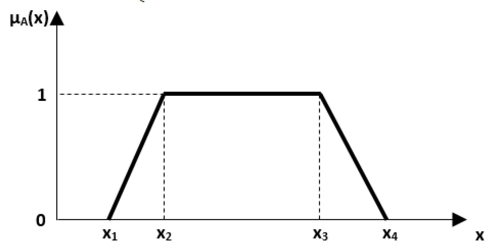
The Decision-Maker will calculate the break points based on the statistical parameters of the clusters (determined in the above stage) which define the linguistic categories of each input variable (the active and reactive powers injected by the wind farms and requested at the level of the buses) and output variables (tap position of each power transformer and total power losses).
The proposed approach takes into account the fuzzy numbers of linguistic categories associated with the input and output variables, which are composed of very small, small, medium, high, and very high. To define the linguistic categories' meaning, the trapezoidal membership functions with various values of the break points must be employed.
3.2.2. Improving Fuzzification Process with Fuzzy K-Means Clustering Algorithm
Fuzzy K-means is a clustering algorithm that allows an element in the data set to belong to one or more groups with a specific membership degree. Often employed in pattern recognition, this method minimizes the following objective function [37].
where: m – is the hyper-parameter having as aim how fuzzy the cluster will be; μkv –the membership degree of an object/element from the database ev, v = 1, …,E, to cluster k; ck – the centroid of the cluster k; ║*║- represents any norm that expresses the similarity measure between any element ev and the centroid of a cluster k, k = 1, …, K.
Fuzzy clustering corresponds to an iterative optimisation process that minimises the objective function (15). The membership degree uvk and the centroid cjk are updated using the following relations.
The clustering process will stop when the following condition is fulfilled.
where ε is associated with the stop criterion and it is assigned to an iteration.
If the assumption that each point within a cluster can be a potential centre is used, the algorithm considers the following steps [37,38,39]:
- The density of the nearby data points must be calculated to determine the likelihood that each point in a cluster will become a centre.
- Choose the data point with the highest chance of becoming the cluster's first centre.
- Remove all the data points near the cluster's first centre based on the influence range around the cluster's first centre.
- After that, choose the cluster's remaining point with the greatest likelihood of becoming its next centre.
- Repeat the steps 3 and 4 until all of the data within the cluster's influence range is obtained.
For a better understanding, the following example considers the one-dimensional space determined by the elements of a data set, as seen in Figure 4. In Figure 5, the element indicated by the arrow belongs more to Cluster B than Cluster A. The value 0.25 suggests the respective element's membership degree to group A.
3.2.3. Inference Engine
The fuzzy outputs of the inference engine is dependent on the application of the relevant rules to the fuzzy inputs. These rules are used to map the linguistic values to a fuzzy set, which necessitates the transformation of these values into a crisp value [40].
The linguistic fuzzy rule is a type of rule that describes a domain's knowledge by establishing the relationship between output and input variables.
An example of a fuzzy inference rule belonging to the proposed FIS can be represented by the following expression:
Rule Rn:
IF PWFinj is LCPinji AND QWFinj is LCQinjj AND ……. AND PPQ_busreq is LCPreql
AND QPQ_busreq is LCQinjo THEN TPTr is LCTPk AND… AND Γ is LCΓs
where: Rk is the k-th rule from FIS, PWFinj, QWFinj, PPQ_busreq, QPQ_busreq represent the input variables considered in the OPF problem (the active and reactive powers injected by the wind farms and requested at the level of the buses) considered as the linguistic categories; LCPinji, LCQinjj,, LCPreql, LCQreqo, i {1, …, NPinjLC}, j {1, …, NQinjLC}, l {1, …, NPreqLC}, o {1, …, NQreqLC} are the linguistic categories of the input variables; NPinjLC, NQinjLC, NPreqLC and NQreqLC indicate the maximum number of the linguistic categories associated with the input variables; TPTr, Tr = 1, …, NT, and Γ are the output variable (plot positions of the power transformers and power losses from the electric network; LCTPk and LCΓs, k {1, …, NTP}, s {1, …, NΓ} corresponds to the linguistic categories of the output variables.
The components IF and THEN from the relation (19) are known as antecedent and consequent, respectively. Whenever a value is provided as an input to the fuzzy inference engine, it's fuzzified using the trapezoidal membership function that the Decision-Maker specifies. These functions are based on various linguistic categories and can be used to map multiple numerical inputs to fuzzy numbers. The operators used in the fuzzy inference engine are AND and OR. As seen in relation (19), the proposed FIS used only the AND operator. The concept of the fuzzy "and" operator is defined as follows.
The rule extracts the minimum number of membership values. The inference process includes the following steps [41]:
- Calculate the inputs' compatibility with the first component (antecedent) of the inference rule Rn, n = 1, ..., NR.
- Identifying the set of rules RSR closest to the input variables with the highest degree of compatibility. Each of the input data subsets will have a single rule.
- Corresponding to RSR, calculate the membership of input variables in its linguistic categories and choose the higher one as the degree of firing of the rule.
- Fire the rules in RSR and apply the defuzzification process considering the linguistic output value of each rule and its corresponding degree of firing.
3.2.4. Defuzzification Process
The output associated with a crisp value of our proposed FIS is obtained by using the centroid method based on the following relation [33,34,40,41,42]:
The centroid method uses the mass centre, represented as z, to determine a single scalar value in a fuzzy output distribution. The other variables in the relationship refer to: μc corresponds to the membership of the fuzzy sets, and Mj represents the value of the membership. Ultimately, the crisp outputs are approximations of the tap positions of the power transformers and power losses from the electric network.
4. Case Study
The FIS-based Optimal Power Flow analysis was tested in a real electric network integrating two wind power farms representing a zone from the Romanian power system [28]. The network contains buses with two voltage levels (Ultra High and High) connected through eight electric lines and three power transformers, see Figure 6. The Buses 2, 3, 4, 6, 7, 8, and 10 have the high voltage level (identified with the red colour), and 1, 5, and 9 are associated with the ultra-high voltage level (colour blue in the figure). Bus 1 corresponds to the slack bus in steady-state calculations performed by the Transmission Network Operator. Between buses 1 and 2, 5 and 6, and 8 and 9, respectively, are the power transformers with the rated power of 200 MVA having On-Load Load Tap Changers with 25 taps (tap 13 corresponds to the median position). Table 2 presents the technical characteristics of the electric lines. The injected power of the two wind farms (with an installed power of 50 MW) through two short-length electric lines is at the level of buses 6 and 8.
The membership functions of all the input variables associated with the proposed FIS were derived from the outputs of the fuzzy K-means-based clustering process which used the information uploaded from the DNO and TNO's SCADA database during the autumn season (September – November) containing 90 days, which hour-by-hour recorded active and reactive powers injected by the two wind farms and requested at the level of the PQ-type buses.
For each hour from the analysed period, an OPF analysis based on the Successive Quadratic Programming (SQP)-based method was performed to determine the optimal solution associated with the tap positions of the three power transformers, leading to the minimum total power losses in the electric network. The obtained values for the total power losses represent the input data for the clustering process to determine the clusters associated with the linguistic categories of the output variable of the FIS. Regarding the tap positions, the linguistic categories are established in relation to the median tap, down and up compared to it (details are highlighted in the fuzzification stage).
Figure 7 and Figure 8 presents the clusters obtained from the K-means algorithm-based clustering processes for the active and reactive power requested at the level of the PQ-types buses (2, 3, 4, 6, 7, 8, 9, and 10) and the active and reactive power injected by the two WFs at the level of the buses 6 and 8 in the analysed period.
Table 3 presents the statistical parameters of the clusters representing the linguistic categories assigned to each input and output data. Each obtained cluster corresponds to a linguistic category associated with the input variables, represented by the active and reactive power requested at the level of the PQ-types buses and the active and reactive power injected by the WFs, of the FIS.
Figure 9 presents the clusters associated with the total power losses (representing the output variable of the FIS) obtained from the clustering process.
Each cluster resulting from the fuzzy K-means algorithm-based clustering process represents a linguistic category which characterizes input or output variables (the requested active and reactive powers at the PQ-type buses and injected active and reactive powers) and output variables (the control variables corresponding with the three tap positions belonging to the power transformers) and values of the objective function represented by the total power losses in the electric network). Table 4 presents the break points of the trapezoidal membership functions associated with the linguistic categories of the input and output variables. Figure 10, Figure 11, Figure 12, Figure 13, Figure 14 and Figure 15 show the shape of the membership functions for the input and output variables included in the FIS proposed to solve the OPF problem.
The signification of the acronyms used in the linguistic categories of the power losses and injected and requested active and reactive powers are: VVS – Very Very Small, VS – Very Small, M –Medium, H – High, and VH – Very High. Regarding the tap positions of the power transformers, the acronyms used in the linguistic categories took into account the location in relation to the median tap (13), down and up: VFD – Very Far Down, FD – Far Down, LFD – Little Far Down, LCD – Little Close Down, CD – Close Down, VCD – Very Close Down, VCU – Very Close Up, CU – Close Up, LCU - Little Close Up, LFU - Little Far Up, FU – Far Up, and VFU – Very Far Up.
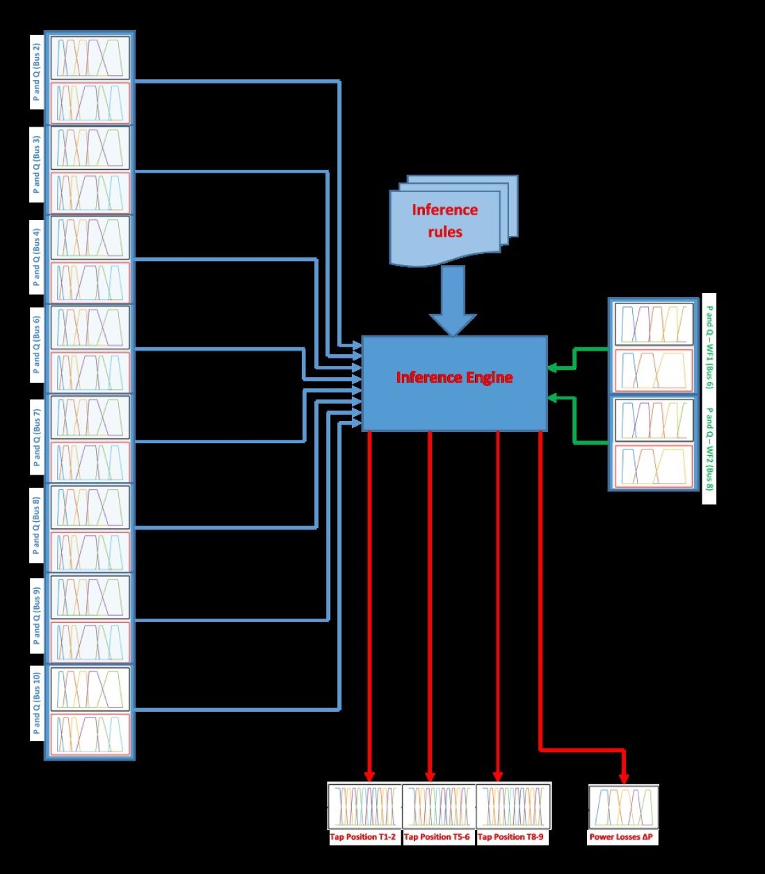
Figure 16 presents the structure of the proposed FIS developed in Matlab, which included the 16 fuzzy inputs corresponding to requested active and reactive powers at the PQ-type buses (2, 3, 4, 6, 7, 8, 9, and 10 and injected active and reactive powers of the two WFs, located in the left part, the fuzzy outputs correspond to the control variables (three positions of the taps belonging to the power transformers) and objective function (total power losses in the electric network), placed at the bottom of the figure, and the inference engine. The inference engine includes 41 fuzzy inference rules, which have a structure similar to expression (19) Table 5 consists of the linguistic categories of the antecedent variables connected by logical AND operation and integrated into each rule, and Table 6 includes the characterization of the linguistic categories assigned with the consequent variables from each rule.
The FIS was subjected to comprehensive characteristic three-day tests, identified as analysis cases D1, D2, and D3, to thoroughly highlight its performance under different injection active power profiles of the two WFs in the database. This thorough testing, as depicted in Figure 17, Figure 18 and Figure 19, provided a detailed understanding of the normalized typical injected power profiles corresponding to the operating regimes of the WFs.
The hourly requested active and reactive powers at the PQ-type buses recorded slight hourly variations, such that they were assigned to the same linguistic categories in the three test days. This comprehensive analysis underscored the differences between the operating regimes of the electric network influenced by the injected power profiles of the two WFs.
In the following, the results obtained (the control variables and the values of the objective function represented by the power losses) using the proposed FIS for the three analysis cases, D1, D2, and D3, are presented in Table 7, Table 8 and Table 9. The tables also indicate the values of the control variables and objective function obtained with the Successive Quadratic Programming (SQP)-based approach (representing one of the best optimization methods proposed in solving the OPF problem) [28,29] and the recalculated values of the objective function with the Newton-Raphson method considering the tap positions obtained with the FIS.
The data analysis from the tables indicates that the values obtained for the control variables using the FIS-based approach occur at the same hour, and the power transformer is either higher or lower by a maximum of one step than in the SQP-based approach. Regarding the objective function, it is close between the two approaches. However, the improved variant of the FIS approach (I-FIS) included an additional steady-state calculus based on the Newton-Raphson method, considering the tap positions determined with FIS have been analysed to verify if the performance of the estimation process associated with the power losses can be increased.
A statistical analysis that utilizes the boxplot representation can highlight the variations of the power losses in the analysis cases associated with the three characteristic days. The boxplots can help in understanding process of the differences between the results obtained with the three approaches (FIS, I-FIS, and SQP). The boxplot shows the distribution values of the minimum (Q0), first (Q1), second (Q2), third (Q3), and maximum (Q4) quartiles [43,44], see Figure 20 and Table 10.
The median value of the power losses voltage, assigned to the red line from inside each of nine boxes, has an increased trend from D1 to D3. The diagram's blue colour highlights the boxes' lengths. The interquartile ranges, represented by the lower and upper sides (Q1 and Q3) of the box, of the different characteristic days are generally similar regardless of the three approaches. But, there are differences between the three days, with higher interquartile ranges for D2 and D3.
If the ENO considers as the time reference the analysed period (in our case a day) then the energy losses should be calculated. Figure 21 presents the energy losses calculated considering the three approaches for each characteristic day.
The results highlighted a minimal difference between the values. Thus, the errors calculated between the SQP, considered as the reference, and the FIS and I-FIS-based approaches were 5.72% and 2.41% for D1, 1.07% and 1.19% for D2, and 1.61% and 1.33% for D3. Even if the errors are slightly higher on the first characteristic day, the proposed approaches can be used successfully by the ENOs in the optimal operation of the electric network. Their practicality is reassured by the main advantages, particularly the lack of an optimization process for determining the values of the control variables (tap positions and the estimation of the power losses). These values are obtained through the inference rules or the simple steady-state calculations based on the Newton-Raphson method.
Finally, the efficiency of the electric network has been calculated with relation (12) and presented in Table 11.
The performance of the proposed approaches (FIS and I-FIS) has been analysed based on the two metrics: percentage error (PE) and average percentage error (APE).
where EEN,h(SQP) represents the efficiency of the electric network calculated with the SQP-based approach, considered as the reference, at the hour h, h = 1, …, NH; EEN(M) is the efficiency of the electric network calculated with the approach M determined at the hour h, h = 1, …, NH, , where M {FIS-based approach, improved FIS-based approach}.
Table 12 and Figure 22, Figure 23 and Figure 24 present the PEs obtained in the analysis cases corresponding to the three characteristic days.
The PE values fall between 0.01% and 0.21% for the characteristic days D1 and D3 and between 0.0% and 0.13% for the characteristic days D1 when the FIS-based approach is applied. When the I-FIS-based approach is applied, the PE values are slightly smaller, with values below 0.07% for the characteristic days D2 and 0.03% for the characteristic days D1 and D3.
The values of the APEs calculated in the cases of characteristic days D1 and D3 when the FIS-based approach has been applied are 0.06%, and for characteristic day D2, 0.04%. The smaller values are recorded for the I-FIS-based methods, regardless of the characteristic day, being equal to 0.01%.
5. Discussions and Conclusions
The OPF analysis helps the ENOs to establish the best operational conditions of electric networks, determining the optimal values of state variables to improve (minimise or maximise) one or more objectives (technical, economic, or environmental). The OPF considers control variables within predetermined limitations and develops effective resource planning strategies. Thus, various approaches have been employed to investigate the uncertainty propagation of electric networks' data input power flow. Unfortunately, the available data and the test networks used, in which researchers made numerous assumptions regarding the generation sources and nodal loads to verify the performance of the fuzzy models, may not provide sufficient confidence that these can be utilised in real applications integrated into electric networks incorporating renewable energy sources.
In this context, the paper proposed an innovative solution to the OPF problem represented by the optimal voltage control from the electric networks integrating wind farms. Based on an FIS implemented in Matlab, this solution is a novel approach to the OPF analysis. It considers the load requested at the PQ-type buses and the powers injected by the generation sources as the fuzzy input variables of the OPF analysis. The FIS determines the suitable tap positions for the power transformers to lead at the minimum active power losses based on the fuzzy rules using the Mamdani inference method. The fuzzy modelling of the input and output variables is done using the fuzzy K-means clustering method, which allows for improving the definition of the trapezoidal membership functions associated with the linguistic categories. Also, an improved variant of the FIS (I-FIS) has been tested, including an additional steady-state calculus based on the Newton-Raphson method, considering the tap positions determined with FIS, to verify if the performance of the estimation process associated with the power losses can be increased. Regarding I-FIS approach, a shortcoming associated with the steady-state calculation can be highlighted, which can lead to additional time spent estimating the power losses.
By enhancing the fuzzy models of the input and output variables, the proposed FIS and I-FIS approaches increase confidence in the decision-making process regarding the tap positions of the power transformers, with a high impact on the operation regimes of the electric networks by reducing power losses.
To test the proposed approach, a real 10-bus network integrating two wind farms, representing a zone from the Romanian power system, has been used. The input data of the clustering process, containing the active and reactive powers associated with the two wind farms and the PQ-type nodes, have been uploaded from the SCADA system.
The FIS has 20 input fuzzy variables (16 associated with the requested active and reactive powers at the level of 8 PQ-type buses and four corresponding to the injected active and reactive powers of the two WFs), four fuzzy output variables (the tap positions of the three power transformers and the power losses), and 41 inference rules. The FIS was subjected to comprehensive characteristic three-day tests, identified as analysis cases, to thoroughly highlight its performance under different injection active power profiles of the two WFs in the database. The results obtained from the FIS and I-FIS-based approaches have been compared with those of the best methods in the mathematical programming category, the SQP-based approach [28,29].
The analysis outcomes indicated that the values obtained for the control variables using the FIS-based approach occur at the same hour, and the power transformer is either higher or lower by a maximum of one step than in the SQP-based approach. Regarding the objective function, it was close between the three approaches, with a slight increase recorded for the FIS approach in the case of the first characteristic day, D1.
If the EDO is considered the time reference for the analysed period, then the analysis of the energy losses highlights the minimal difference between the values. Thus, the errors calculated between the SQP-based approach, considered as the reference, and the FIS and I-FIS-based approaches were 5.72% and 2.41% for D1, 1.07% and 1.19% for D2, and 1.61% and 1.33% for D3. Even if the errors are slightly higher on the first characteristic day, the proposed approaches can be used successfully by the ENOs in the optimal operation of the electric network.
The impact of the OPF by calculating the efficiency of the electric network revealed that percentage errors fall between 0.01% and 0.21% for the characteristic days D1 and D3 and between 0.0% and 0.13% for the characteristic days D1 when the FIS-based approach is applied. I-FIS-based approach led to the percentage errors being slightly smaller, with values below 0.07% for the characteristic days D2 and 0.03% for the characteristic days D1 and D3. The average percentage of errors has been between 0.04% and 0.06 in the case of the FIS-based approach and 0.01% for the I-FIS-based approach, regardless of the characteristic day.
The practical implementation of the two proposed approaches is supported by the main advantages, particularly the efficiency and absence of an optimization process for determining the control variables' values (the transformers' tap positions) and the power losses. These values are derived from the inference rules and straightforward calculations associated with the steady-state regimes based on the Newton-Raphson method. However, we must also consider the burden of the practical implementation of the FIS, which could be associated with the input variables, depending on the number of the PQ-type buses and WFs from the electric network analysed.
Future work involves integrating more renewable energy sources modelled in the FIS and testing on more electric network topologies, increasing confidence in the practical implementation of the approaches.
Author Contributions
Conceptualization, G.G. and B.L.; methodology, G.G. and B.L.; software, G.G.; validation, B.N. and B.L.; formal analysis, B.L. and B.N.; investigation, B.L. and B.N.; resources, G.G.; data curation, G.G.; writing—original draft preparation, G.G., B.N. and B.L.; writing—review and editing, G.G. and B.N.; visualization, G.G.; supervision, G.G.; project administration, G.G.; funding acquisition, G.G. All authors have read and agreed to the published version of the manuscript.
Funding
This research received no external funding.
Informed Consent Statement
Not applicable.
Data Availability Statement
The original contributions presented in the study are included in the article, further inquiries can be directed to the corresponding author.
Acknowledgments
In this section, you can acknowledge any support given which is not covered by the author contribution or funding sections. This may include administrative and technical support, or donations in kind (e.g., materials used for experiments).
Conflicts of Interest
The authors declare no conflicts of interest.
Abbreviations
The following abbreviations are used in this manuscript:
| OPF | Optimal Power Flow |
| FIS | Fuzzy Inference System |
| I-FIS | Improved Fuzzy Inference System |
| ENO | Electric Network Operator |
| SQP | Sequential Quadratic Programming |
| STATCOM | Static Synchronous Compensator |
| CPP | Classical Power Plant |
| WF | Wind Farm |
| OLTC | On-Load Tap Changer |
| PE | Percentage Errors |
| APE | Average Percentage Errors |
| SCADA | Supervisory, Control, and Data Acquisition |
| RES | Renewable Energy Sources |
References
- Risi, B.-G.; Riganti-Fulginei, F.; Laudani, A. Modern Techniques for the Optimal Power Flow Problem: State of the Art. Energies 2022, 15, 6387. [Google Scholar] [CrossRef]
- Momoh, J.A.; Adapa, R.; El-Hawary, M.E. A Review of Selected Optimal Power Flow Literature to 1993. IEEE Transactions on Power Systems, 1999, 14, 96–111. [Google Scholar] [CrossRef]
- Carpentier, J. Contribution á l’Étude du Dispatching Économique. Bulletin de la Société Française des Électriciens 1962, 3, 431–447. [Google Scholar]
- Khalghani, M. R.; Ramezani, M.; Mashhadi, M. R. Probabilistic Power Flow Based on Monte-Carlo Simulation and Data Clustering to Analyze Large-Scale Power System in Including Wind Farm. In Proceedings of the 2020 IEEE Kansas Power and Energy Conference (KPEC), Manhattan, KS, USA; 2020. [Google Scholar]
- Wan, C.; Xu, Z.; Dong, Z. Y.; Wong, K. P. Probabilistic Load Flow Computation Using First-Order Second-Moment Method. In Proceedings of the 2012 IEEE Power and Energy Society General Meeting, San Diego, CA, USA, 2012. [Google Scholar]
- Sun, Y.; Xia, D.; Gao, Z.; Wang, Z.; Li, G.; Lu, W.; Wu, X.; Li, Y. Probabilistic Load Flow Calculation of AC/DC Hybrid System Based on Cumulant Method. International Journal of Electrical Power & Energy Systems, 2022, 139, 107998. [Google Scholar]
- Gallego, L.; Franco, J.; Cordero, L. A Fast-Specialized Point Estimate Method for the Probabilistic Optimal Power Flow in Distribution Systems with Renewable Distributed Generation. International Journal of Electrical Power & Energy Systems, 2021, 131, 107049. [Google Scholar]
- Varathan, G.; Belwin, E. J. A Review of Uncertainty Management Approaches for Active Distribution System Planning. Renewable and Sustainable Energy Reviews, 2024, 205, 114808. [Google Scholar]
- Miranda, V.; Saraiva, J. T. Fuzzy Modelling of Power System Optimal Load Flow. In Proceedings of the Power Industry Computer Application Conference, Baltimore, MD, USA, 1991. [Google Scholar]
- Gomes, B. A.; Saraiva, J. T.; Neves, L. Modelling Costs and Load Uncertainties in Optimal Power Flow Studies In Proceedings of the 5th International Conference on the European Electricity Market, Lisboa, Portugal, 2008.
- Sarcheshmah, M.S; Seif, A.R. A New Fuzzy Power Flow Analysis Based on Uncertain Inputs. International Review of Electrical Engineering, 2009, 4, 122–128. [Google Scholar]
- Salhi, A.; Naimi, D.; Tarek, B. Fuzzy Multi-Objective Optimal Power Flow Using Genetic Algorithms Applied to Algerian Electrical Network. Recent Patents on Electrical Engineering, 2013, 11, 443–454. [Google Scholar] [CrossRef]
- Zhang, W.; Peng, Z.; Wang, Q.; Qi, W.; Ge, Y. Optimal power flow method with consideration of uncertainty sources of renewable energy and demand response. Front. Energy Res. 2024, 12, 1421277. [Google Scholar] [CrossRef]
- Luo, L.; Shi, L.; Ni, Y. A Solution of Optimal Power Flow Incorporating Wind Generation and Power Grid Uncertainties. IEEE Access, 2018, 6, 19681–19690. [Google Scholar] [CrossRef]
- Hassan, M. H.; Kamel, S.; Hussien, A. G. Optimal Power Flow Analysis Considering Renewable Energy Resources Uncertainty Based on an Improved Wild Horse Optimizer. IET Generation, Transmission & Distribution, 2023, 17, 3582–3606. [Google Scholar]
- Lastomo, D.; Setiadi, H. Optimal Power Flow Using Fuzzy-Firefly Algorithm. In Proceedings of the 5th International Conference on Electrical Engineering, Computer Science and Informatics (EECSI), Malang, Indonesia; 2018. [Google Scholar]
- Alizadeh, M. I.; Usman, M.; Capitanescu, F. Toward Stochastic Multi-Period AC Security Constrained Optimal Power Flow to Procure Flexibility For Managing Congestion and Voltages. In Proceedings of the International Conference on Smart Energy Systems and Technologies (SEST), Vaasa, Finland; 2021. [Google Scholar]
- Ilyas, M. A.; Abbas, G.; Alquthami, T.; Awais, M.; Rasheed, M. B. Multi-Objective Optimal Power Flow with Integration of Renewable Energy Sources Using Fuzzy Membership Function. IEEE Access, 2020, 8, 143185–143200. [Google Scholar] [CrossRef]
- Ma, R.; Li, X.; Gao, W.; Lu, P.; Wang, T. Random-Fuzzy Chance-Constrained Programming Optimal Power Flow of Wind Integrated Power Considering Voltage Stability. IEEE Access, 2020, 8, 217957–217966. [Google Scholar] [CrossRef]
- Muangkhiew, P.; Chayakulkheeree, K. Multi-objective Optimal Power Flow Using Fuzzy Satisfactory Stochastic Optimization. International Energy Journal, 2022, 22, 281–290. [Google Scholar]
- Pandiarajan, K.; Babulal, C. K. Fuzzy Harmony Search Algorithm Based Optimal Power Flow for Power System Security Enhancement. International Journal of Electrical Power & Energy Systems, 2016, 78, 72–79. [Google Scholar]
- Yan, Q.; Gao, W.; Ma, R. Multi-Objective Random-Fuzzy Optimal Power Flow of Transmission-Distribution Interaction Considering Security Region Constraints. Electric Power Systems Research, 2023, 224, 109715. [Google Scholar] [CrossRef]
- Kumar, S.; Chaturvedi, D. K. Optimal Power Flow Solution Using Fuzzy Evolutionary and Swarm Optimization. International Journal of Electrical Power & Energy Systems, 2013, 47, 416–423. [Google Scholar]
- Liang, R. H.; Tsai, S. R.; Chen, Y. T.; Tseng, W. T. Optimal Power Flow By a Fuzzy Based Hybrid Particle Swarm Optimization Approach. Electric Power Systems Research, 2011, 81, 1466–1474. [Google Scholar] [CrossRef]
- Mittal, U.; Nangia, U.; Jain, N. K.; Gupta, S. Optimal Power Flow Solution Using a Learning-Based Sine–Cosine Algorithm. The Journal of Supercomputing, 2024, 80, 1–39. [Google Scholar] [CrossRef]
- Ahmadipour, M.; Ali, Z.; Ramachandaramurthy, V. K.; Ridha, H. M. A Memory-Guided Jaya Algorithm to Solve Multi-Objective Optimal Power Flow Integrating Renewable Energy Sources. Applied Soft Computing 2024, 111924. [Google Scholar] [CrossRef]
- Yang, C.; Sun, Y.; Zou, Y.; Zheng, F.; Liu, S.; Zhao, B.; Wu, M.; Cui, H. Optimal Power Flow in Distribution Network: A Review on Problem Formulation and Optimization Methods. Energies 2023, 16, 5974. [Google Scholar] [CrossRef]
- Grigoraș, G.; Neagu, B.-C.; Ivanov, O.; Livadariu, B.; Scarlatache, F. A New SQP Methodology for Coordinated Transformer Tap Control Optimization in Electric Networks Integrating Wind Farms. Appl. Sci. 2022, 12, 1129. [Google Scholar] [CrossRef]
- Hasan, M. S.; Chowdhury, M. M. -U. –T; Kamalasadan, S. Sequential Quadratic Programming (SQP) Based Optimal Power Flow Methodologies for Electric Distribution System with High Penetration of DERs. IEEE Transactions on Industry Applications, 2024, 60, 4810–4820. [Google Scholar] [CrossRef]
- Saatchi, R. Fuzzy Logic Concepts, Developments and Implementation. Information, 2024, 15, 656. [Google Scholar] [CrossRef]
- Gu, X.; Han, J.; Shen, Q.; Angelov, P. . Autonomous Learning for Fuzzy Systems: A Review. Artif Intell Rev 2023, 56, 7549–7595. [Google Scholar] [CrossRef]
- Samavat, T.; Nazari, M.; Ghalehnoie, M.; Nasab, M.A.; Zand, M.; Sanjeevikumar, P.; Khan, B. A Comparative Analysis of the Mamdani and Sugeno Fuzzy Inference Systems for MPPT of an Islanded PV System. International Journal of Energy Research 2023, 2023. [Google Scholar] [CrossRef]
- Pujaru, K.; Adak, D.; Kar, T.K.; Patra, S.; Jana, S. A Mamdani Fuzzy Inference System with Trapezoidal Membership Functions For Investigating Fishery Production. Decision Analytics Journal, 2024, 11, 100481. [Google Scholar] [CrossRef]
- Rizvi, S.; Mitchell, J.; Razaque, A.; et al. A Fuzzy Inference System (FIS) to Evaluate the Security Readiness of Cloud Service Providers. J Cloud Comp, 2020, 9, 42. [Google Scholar] [CrossRef]
- Pathinathan, T.; Ponnivalavan, K.; Mike Dison, E. Different Types of Fuzzy Numbers and Certain Properties. Journal of Computer and Mathematical Sciences, 2015, 6, 631–651. [Google Scholar]
- Grigoraş, G.; Neagu, B.; Scarlatache, F. Estimation of Energy Losses in Distribution Transformers Using A Fuzzy Approach, In Proceedings of the International Symposium on Fundamentals of Electrical Engineering (ISFEE), Bucharest, Romania, 2016.
- Ferraro, M.B. Fuzzy k-Means: History and Applications. Econometrics and Statistics, 2024, 30, 110–123. [Google Scholar] [CrossRef]
- Reddy Poli, V. S. Fuzzy C-Means and Fuzzy K-Means Algorithms using Fuzzy Functional Dependencies, In Proceedings of the 2022 International Conference on Fuzzy Theory and Its Applications (iFUZZY), Kaohsiung, Taiwan, 2022.
- Choudhary, A.; Badholia, A.; Sharma, A.; et al. A Dynamic K-Means-Based Clustering Algorithm Using Fuzzy Logic for CH Selection and Data Transmission Based On Machine Learning. Soft Comput 2023, 27, 6135–6149. [Google Scholar] [CrossRef]
- Surendra, H.J.; Deka, P.C.; Rajakumara, H.N. Application of Mamdani model-based fuzzy inference system in water consumption estimation using time series. Soft Comput, 2022, 26, 11839–11847. [Google Scholar] [CrossRef]
- Nogueira, T. M.; Camargo, H. d. A. Context-Sensitive Clustering in the Design of Fuzzy Models, In Proceedings of the 2008 Eighth International Conference on Hybrid Intelligent Systems, Barcelona, Spain, 2008.
- Cartina, G.; Grigoras, G.; Bobric, E. C.; Comanescu, D. Improved fuzzy load models by clustering techniques in optimal planning of distribution networks. In Proceedings of the 2009 IEEE Bucharest PowerTech, Bucharest, Romania; 2009. [Google Scholar]
- Mazarei, A.; Sousa, R.; Mendes-Moreira, J.; Molchanov, S.; Ferreira, H.M. Online Boxplot Derived Outlier Detection. Int J Data Sci Anal, 2025, 19, 83–97. [Google Scholar] [CrossRef]
- Thirumalai, C.; Kanimozhi, R.; Vaishnavi, B. Data Analysis Using Box Plot on Electricity Consumption, Proceedings of the 2017 International conference of Electronics, Communication and Aerospace Technology (ICECA), Coimbatore, India, 2017.
Figure 1.
The framework of the solutions for OPF problem, adapted after [27].
Figure 1.
The framework of the solutions for OPF problem, adapted after [27].
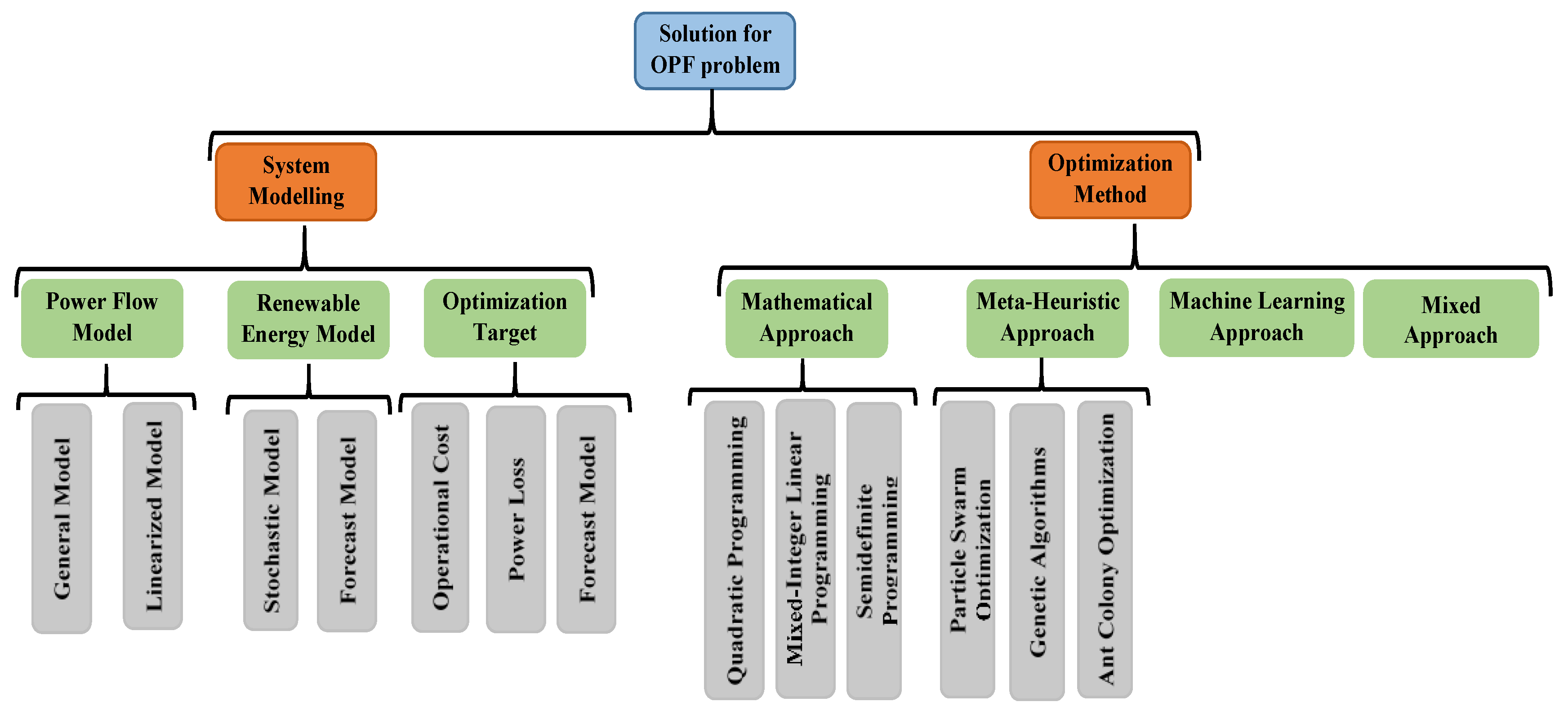
Figure 2.
The basic structure of the FIS.
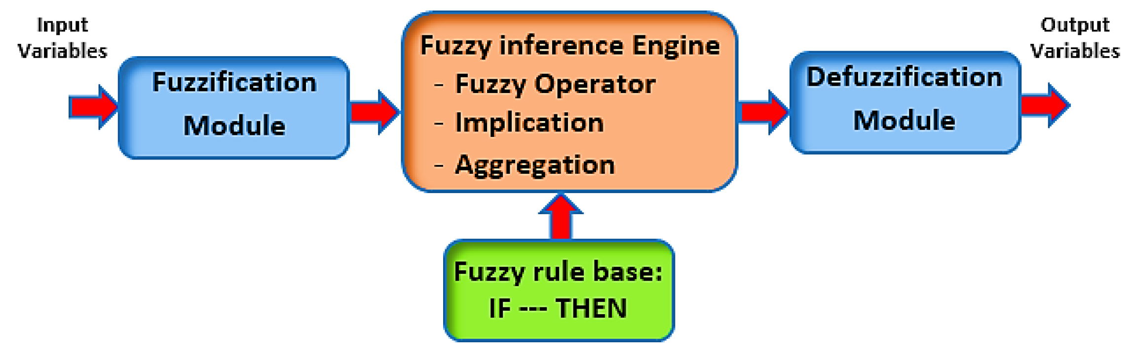
Figure 4.
Trapezoidal fuzzy number.
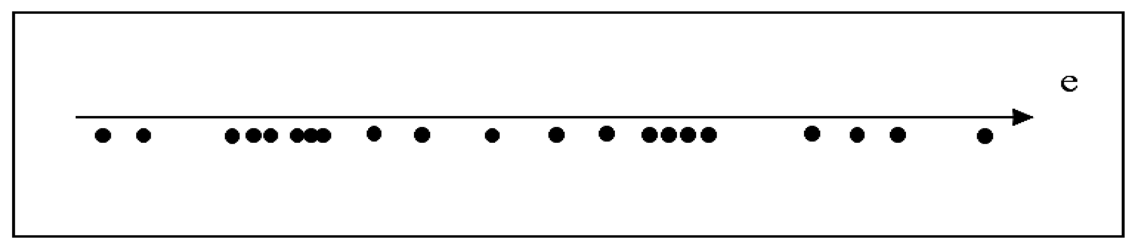
Figure 5.
Membership degrees of the elements determined with the Fuzzy K-means algorithm.
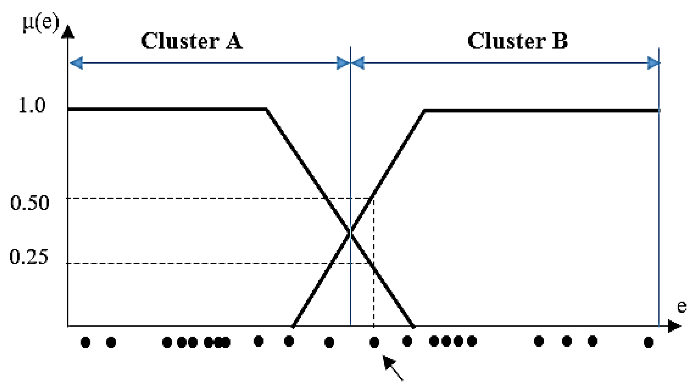
Figure 6.
The test 10-bus electric network [28].
Figure 6.
The test 10-bus electric network [28].
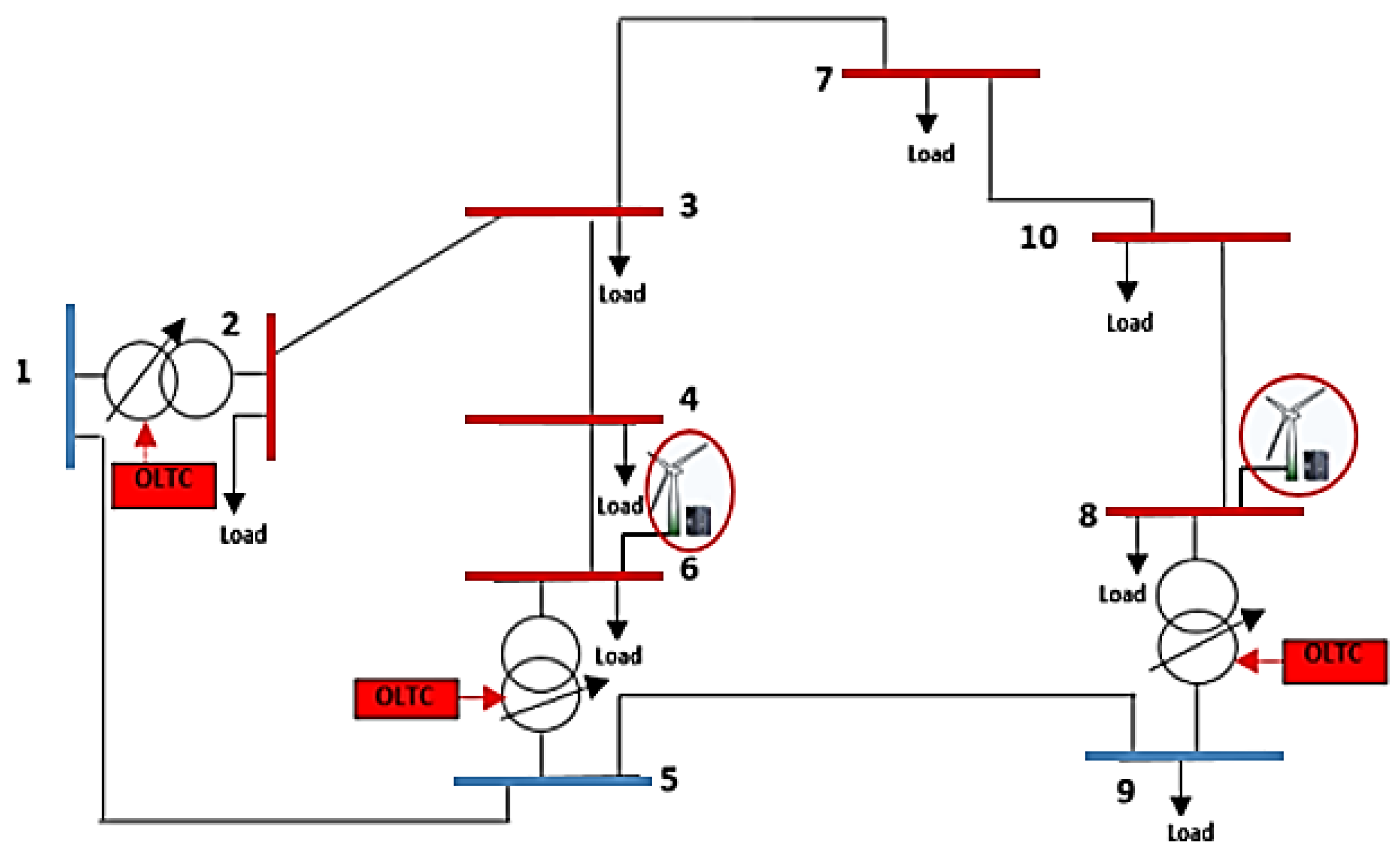
Figure 7.
Representations in one-dimensional space of the clusters resulted from the clustering processes for the requested active power (a) and reactive power (b) at the level of the PQ-type buses.
Figure 7.
Representations in one-dimensional space of the clusters resulted from the clustering processes for the requested active power (a) and reactive power (b) at the level of the PQ-type buses.
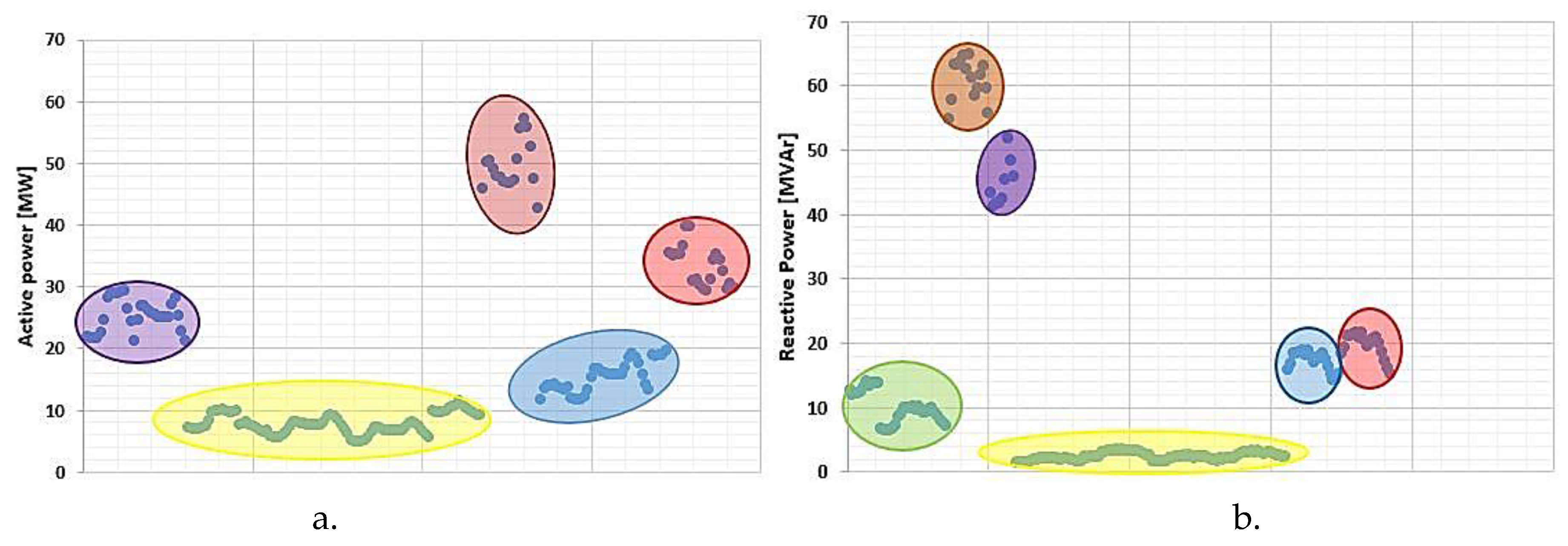
Figure 8.
Representations in one-dimensional space of the clusters resulted from the clustering processes for the injected active power (a) and reactive power (b) by the WFs.
Figure 8.
Representations in one-dimensional space of the clusters resulted from the clustering processes for the injected active power (a) and reactive power (b) by the WFs.
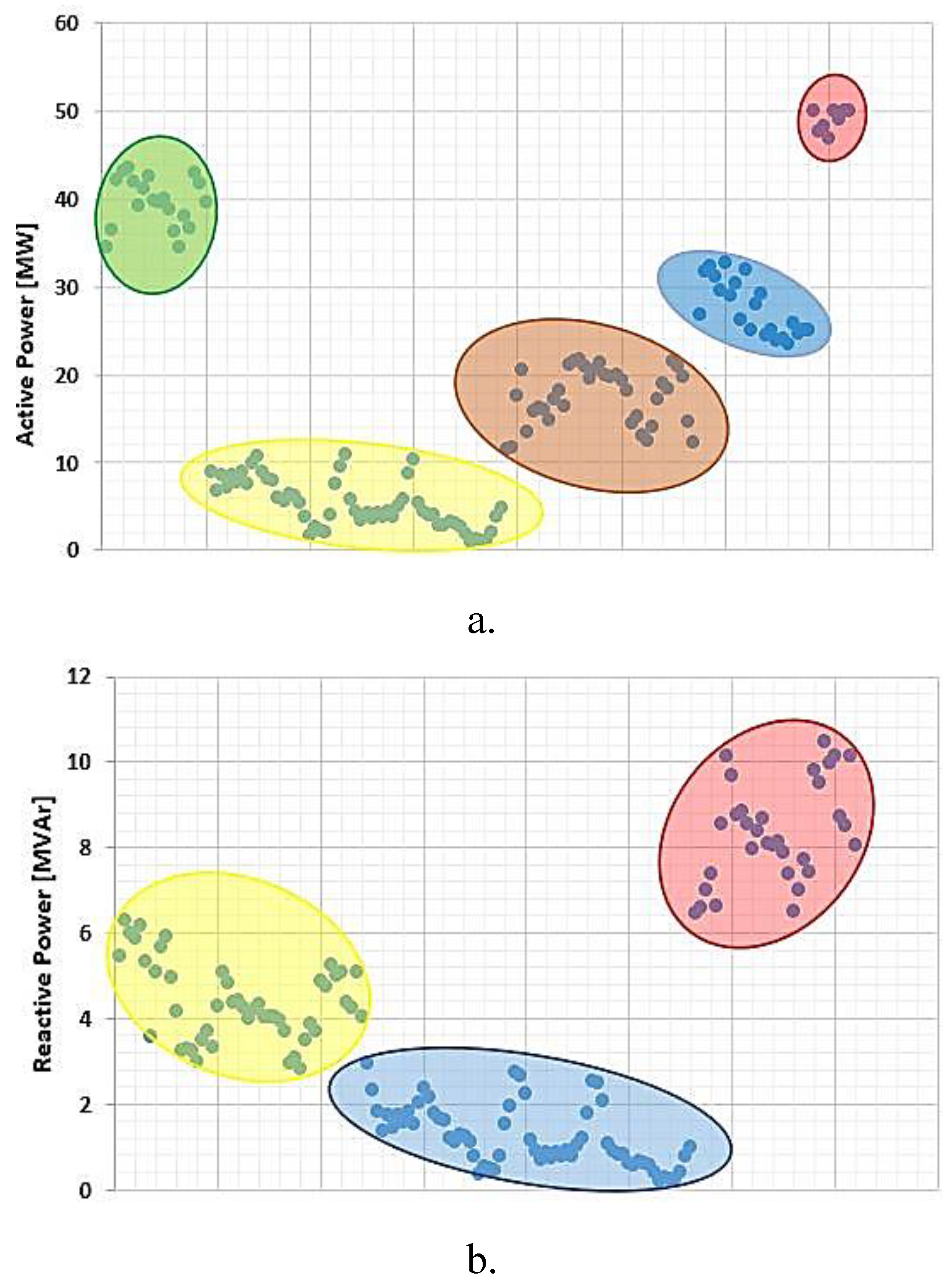
Figure 9.
Representations in one-dimensional space of the clusters resulted from the clustering processes for the total active power losses.
Figure 9.
Representations in one-dimensional space of the clusters resulted from the clustering processes for the total active power losses.
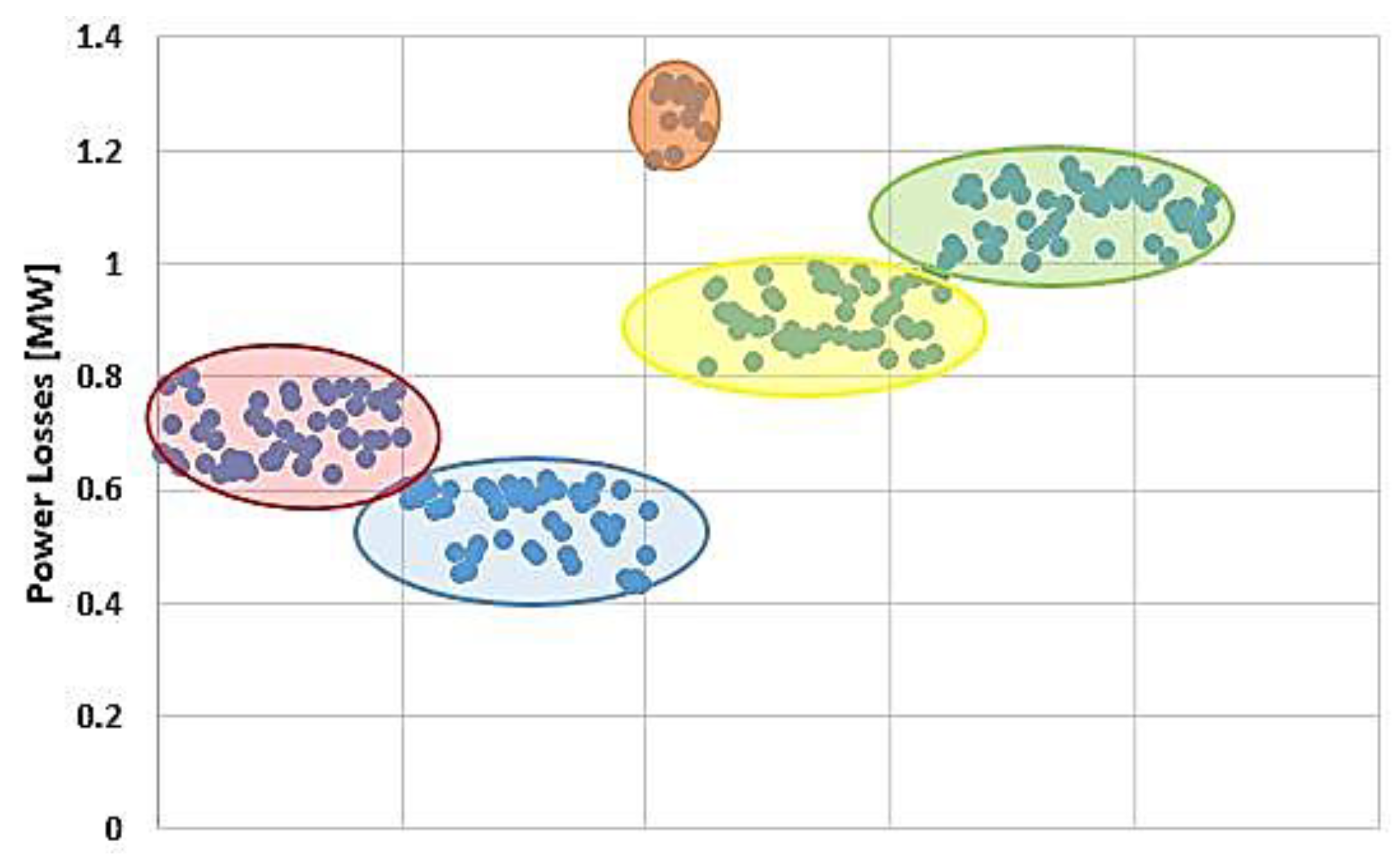
Figure 10.
The membership functions of the linguistic categories associated with the active power in the PQ-type buses.
Figure 10.
The membership functions of the linguistic categories associated with the active power in the PQ-type buses.
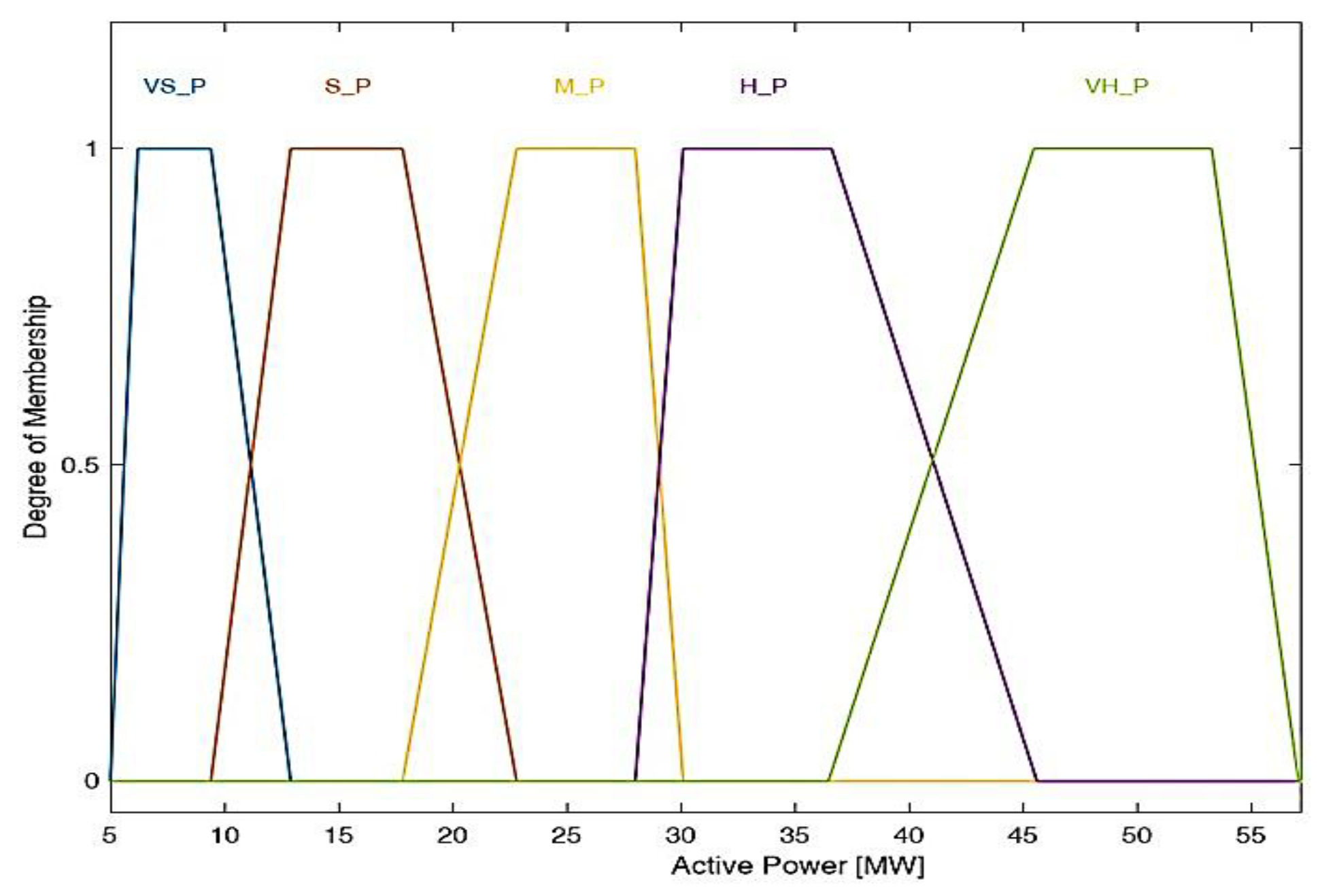
Figure 11.
The membership functions of the linguistic categories associated with the reactive power in the PQ-type buses.
Figure 11.
The membership functions of the linguistic categories associated with the reactive power in the PQ-type buses.
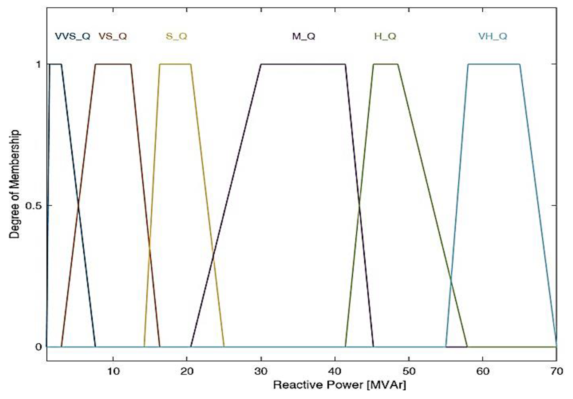
Figure 12.
The membership functions of the linguistic categories associated with the active power generated by the wind farms.
Figure 12.
The membership functions of the linguistic categories associated with the active power generated by the wind farms.
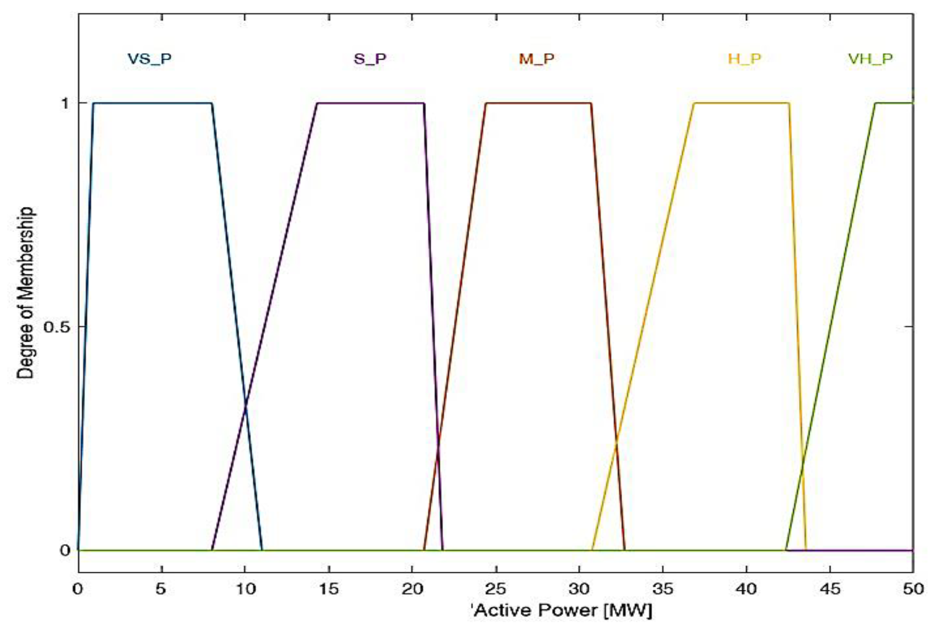
Figure 13.
The membership functions of the linguistic categories associated with the reactive power generated by the wind farms.
Figure 13.
The membership functions of the linguistic categories associated with the reactive power generated by the wind farms.
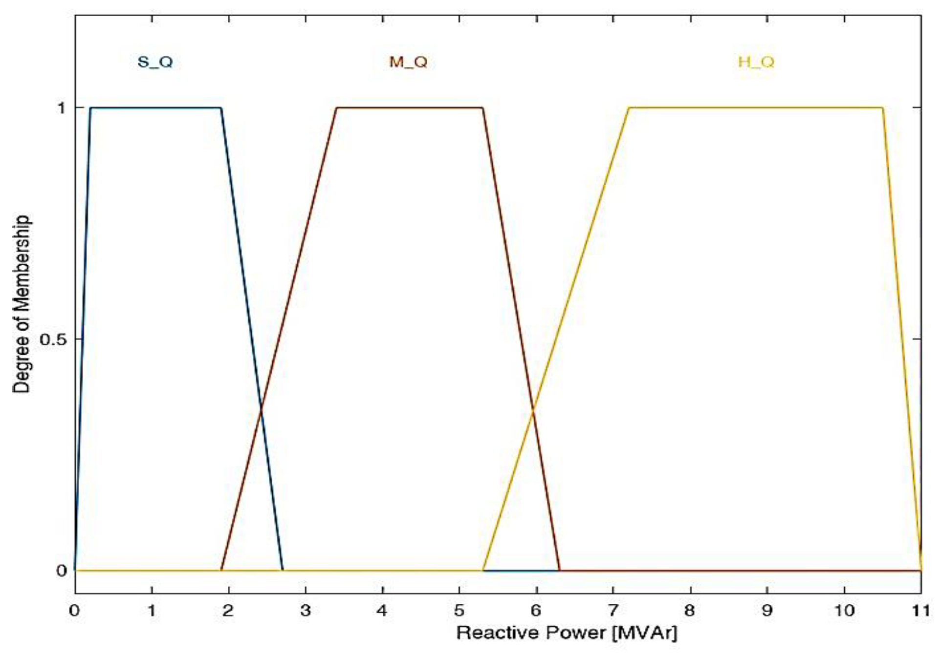
Figure 14.
The membership functions of the linguistic categories associated with the tap positions of the OLTCs corresponding to the power transformers .
Figure 14.
The membership functions of the linguistic categories associated with the tap positions of the OLTCs corresponding to the power transformers .
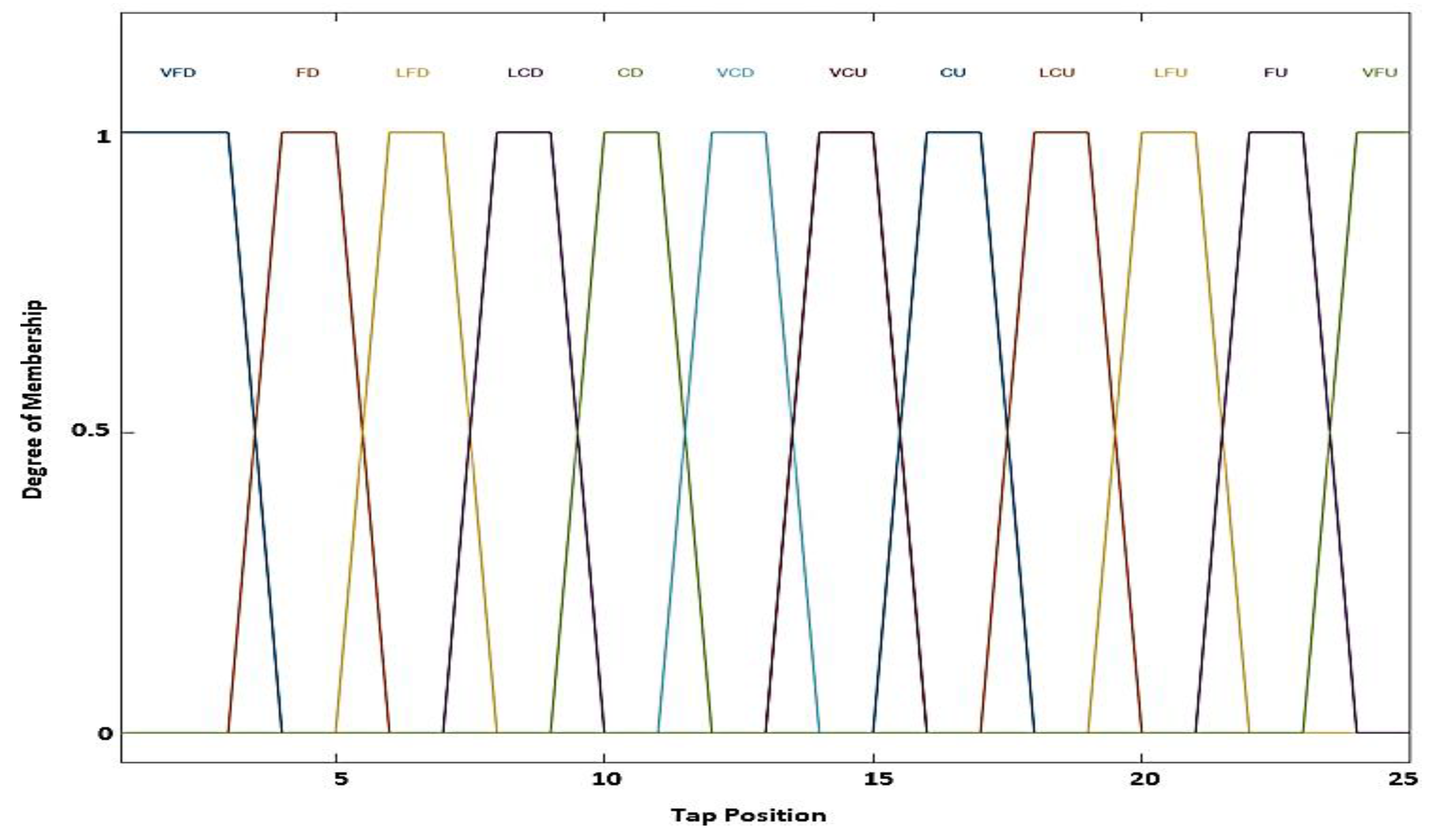
Figure 15.
The membership functions of the linguistic categories associated with the power losses.
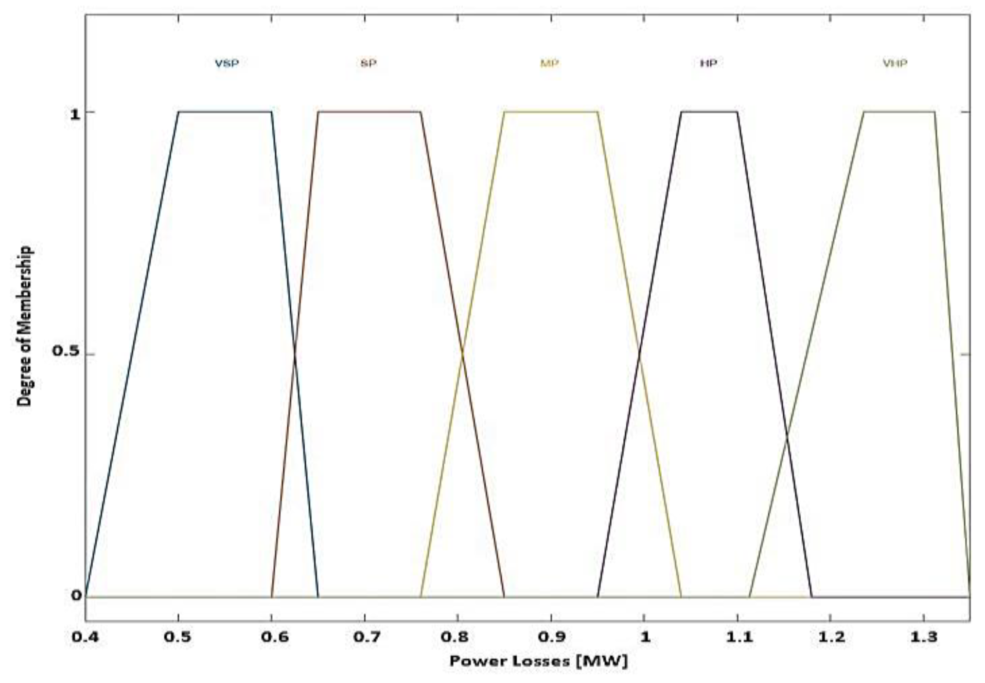
Figure 16.
The structure of the proposed FIS to solve the OPF problem in the test 10-bus network .
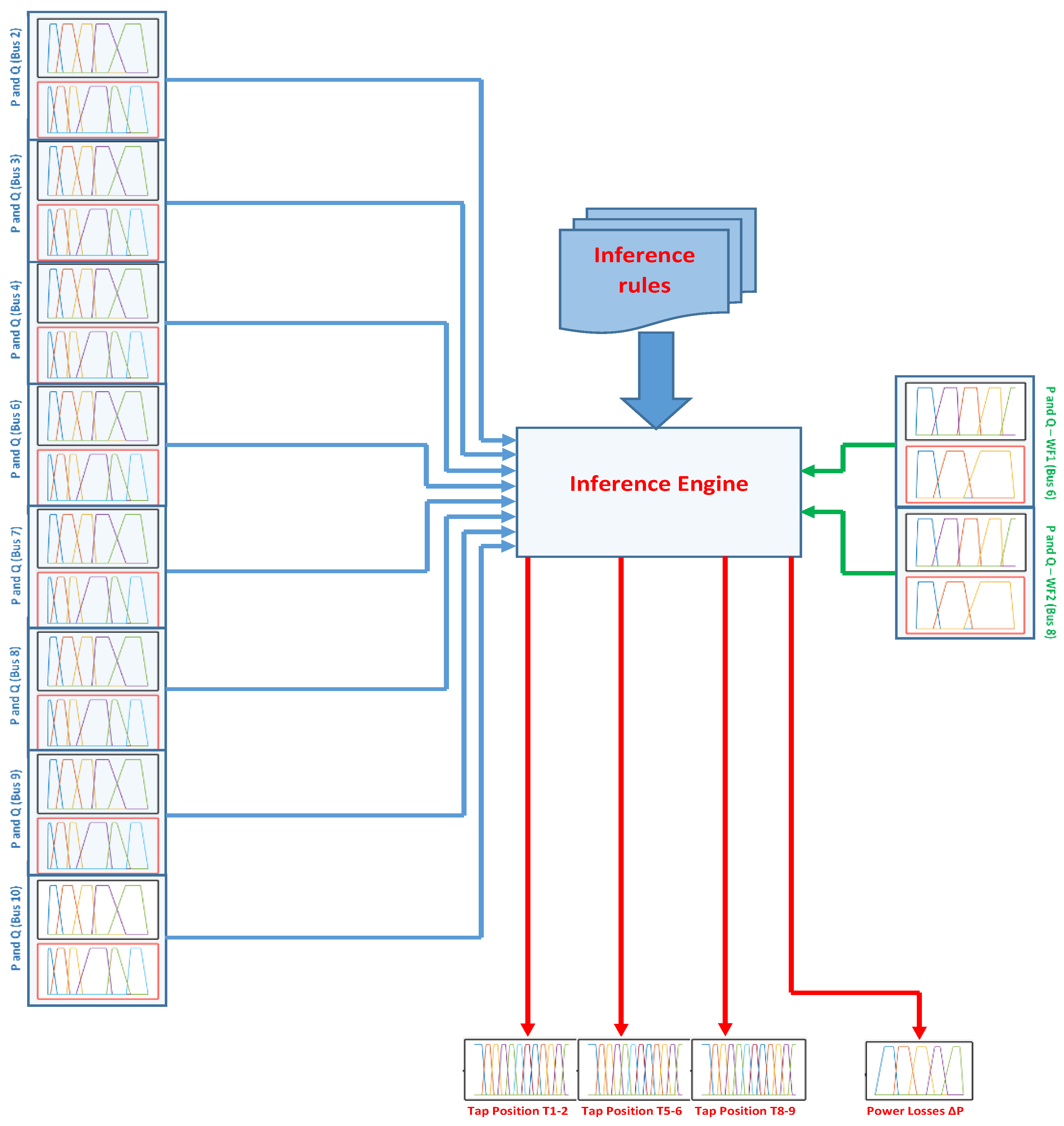
Figure 17.
The normalized typical injected power profiles of the WFs coresponding to the characteristic day D1.
Figure 17.
The normalized typical injected power profiles of the WFs coresponding to the characteristic day D1.
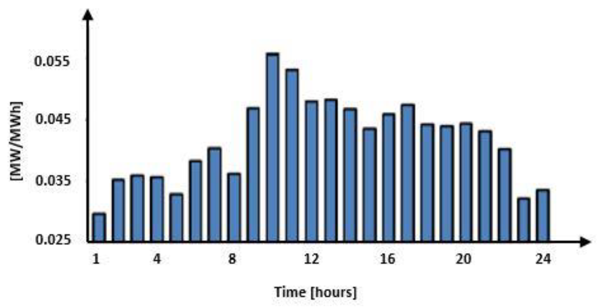
Figure 18.
The normalized typical injected power profiles of the WFs corresponding to the characteristic day D2.
Figure 18.
The normalized typical injected power profiles of the WFs corresponding to the characteristic day D2.
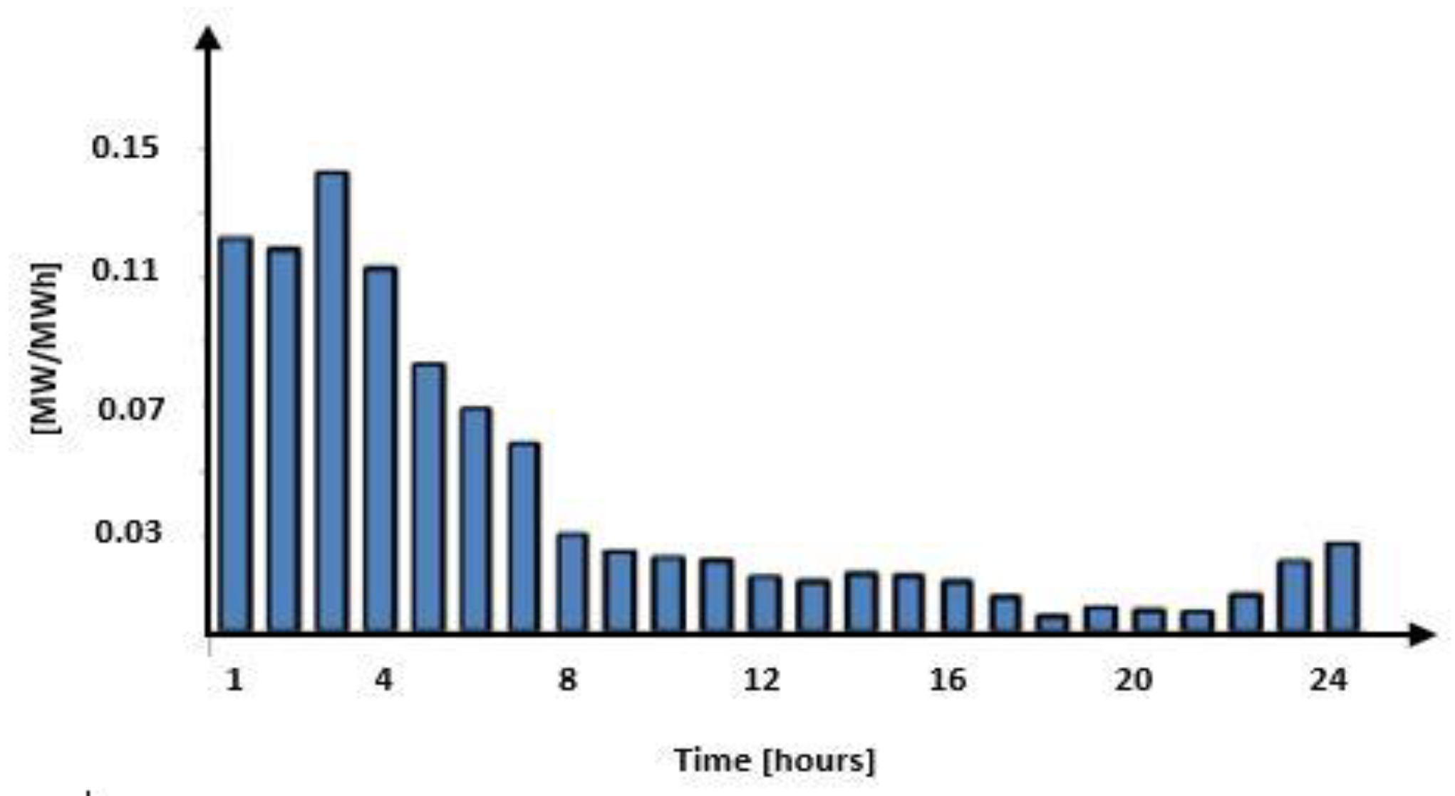
Figure 19.
The normalized typical injected power profiles of the WFs corresponding to the characteristic day D3.
Figure 19.
The normalized typical injected power profiles of the WFs corresponding to the characteristic day D3.
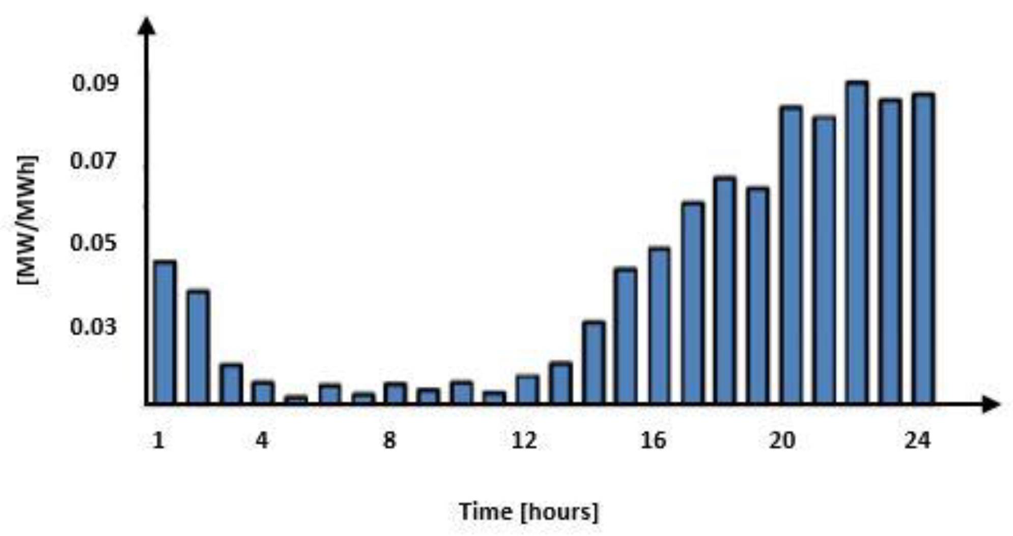
Figure 20.
The boxplot representation of the power losses obtained with the three OPF approaches (FIS, I_FIS, and SQP).
Figure 20.
The boxplot representation of the power losses obtained with the three OPF approaches (FIS, I_FIS, and SQP).
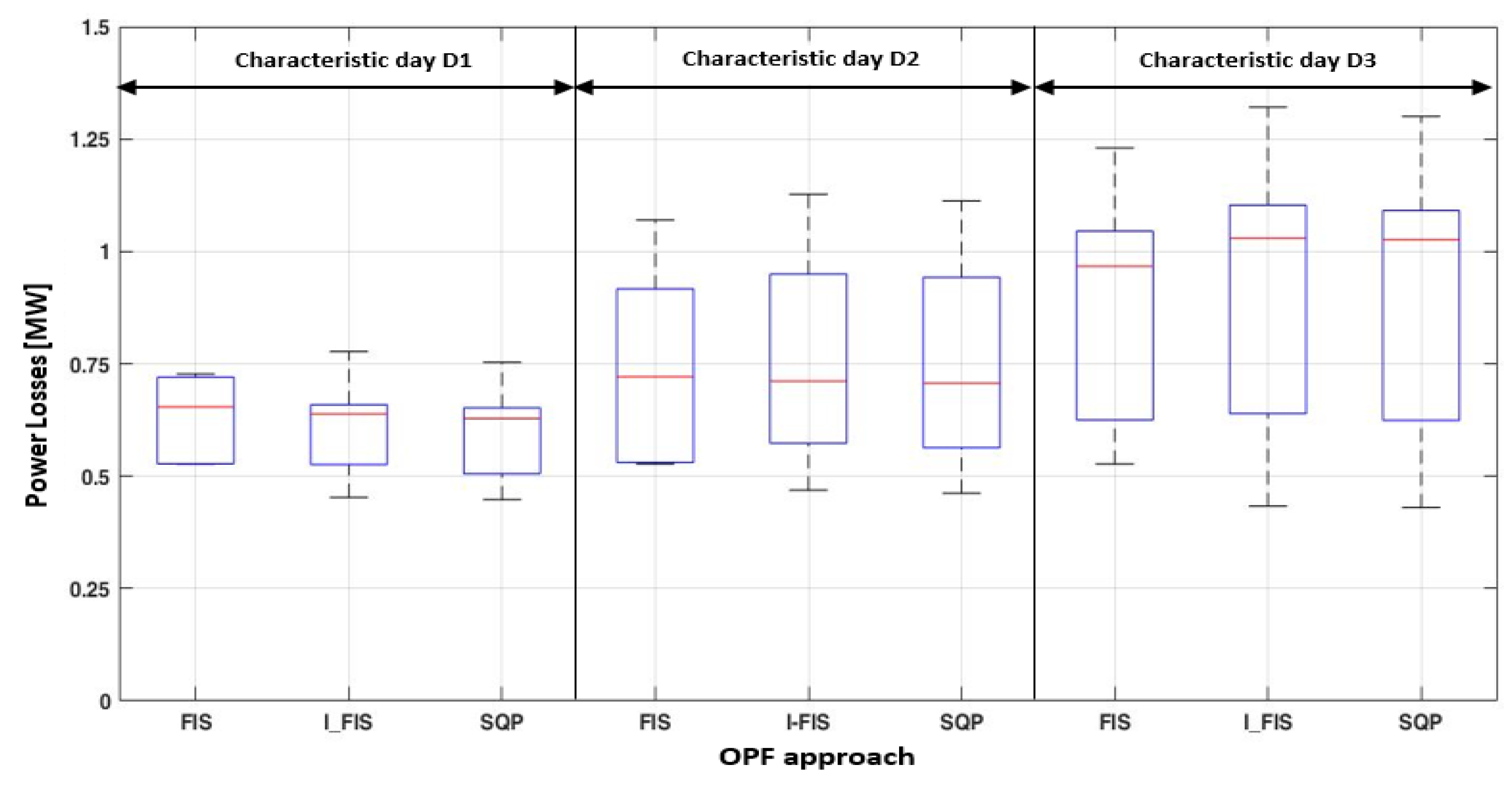
Figure 21.
The energy losses calculated in the three OPF approaches (FIS, I_FIS, and SQP).
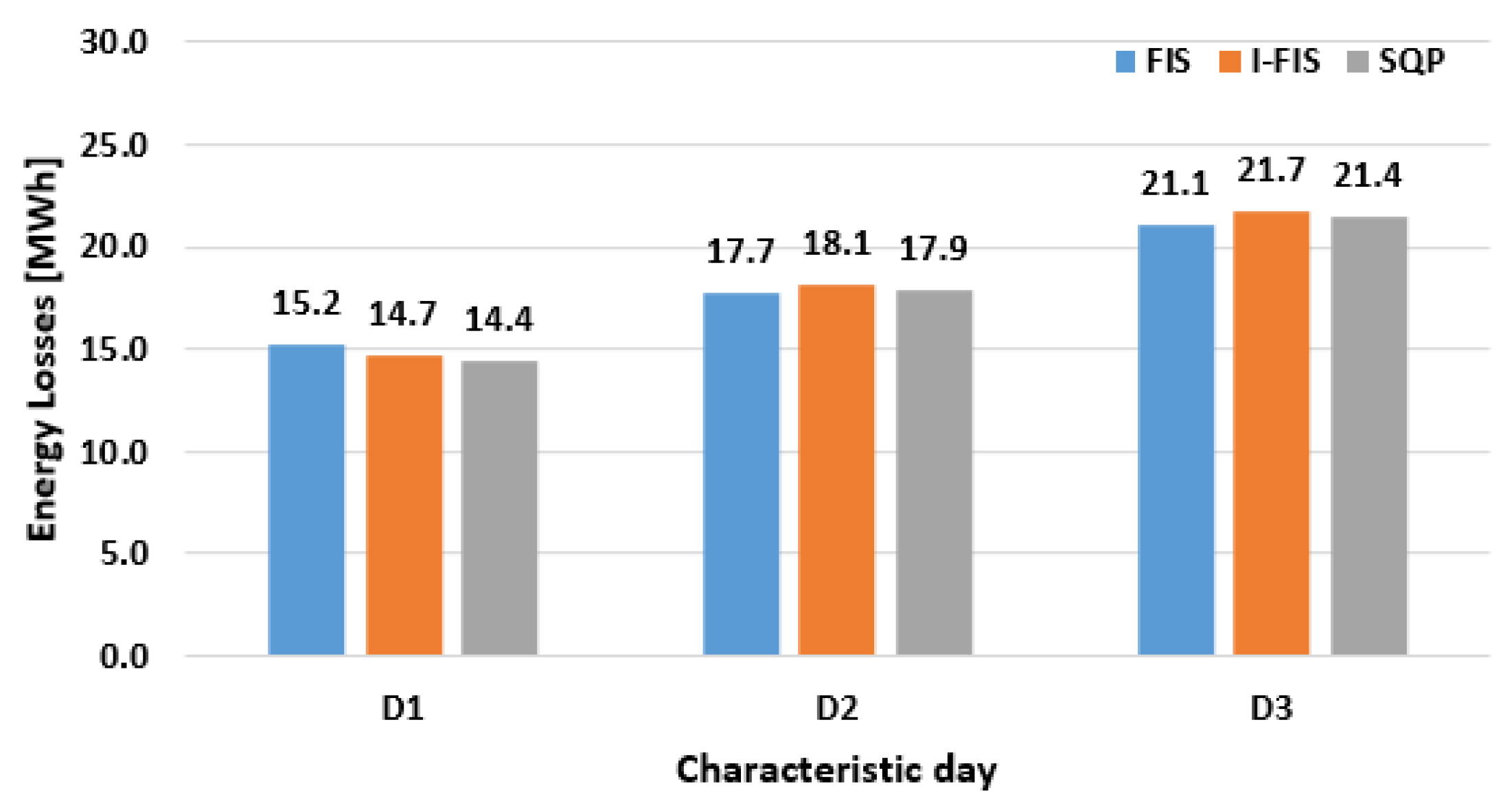
Figure 22.
The percentage errors associated with FIS and I-FIS-based approaches obtained for the characteristic D1, considering SQP-approach as a reference.
Figure 22.
The percentage errors associated with FIS and I-FIS-based approaches obtained for the characteristic D1, considering SQP-approach as a reference.
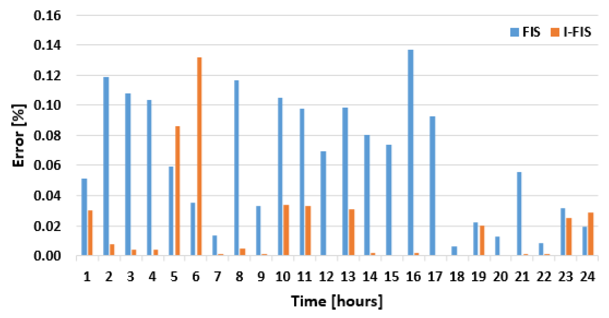
Figure 23.
The percentage errors associated with FIS and I-FIS-based approaches obtained for the characteristic D2, considering SQP-approach as a reference.
Figure 23.
The percentage errors associated with FIS and I-FIS-based approaches obtained for the characteristic D2, considering SQP-approach as a reference.
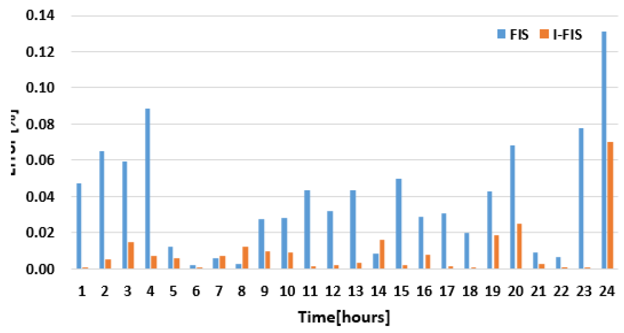
Figure 24.
The percentage errors associated with FIS and I-FIS-based approaches obtained for the characteristic D1, considering SQP-approach as a reference.
Figure 24.
The percentage errors associated with FIS and I-FIS-based approaches obtained for the characteristic D1, considering SQP-approach as a reference.
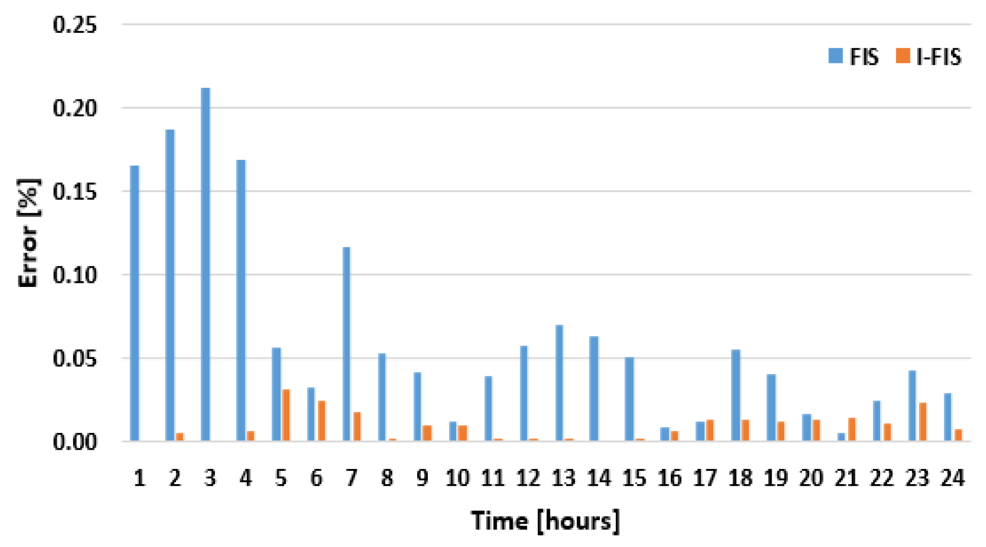

Table 1.
A comparative state of the art between our method and the literature.
| Refs. | Uncertainty data | Defining fuzzy models | Objective Function | OPF Methodology |
Network type |
RES integration |
|
|---|---|---|---|---|---|---|---|
| First | Second | ||||||
| [4] [13] |
Yes | Done by Decision Maker |
Generat. Cost | - | NR-MCS | Real IEEE30 |
Yes |
| [5] | Yes | Done by Decision Maker |
Runtime | - | FOSM-MCS | IEEE9 IEEE18 | No |
| [6] | Yes | Done by Decision Maker |
- | - | CM | IEEE34 IEEE57 | Yes |
| [7] [14] |
Yes | Done by Decision Maker |
Power losses | - | PEM PSO |
IEEE69 IEEE30 |
Yes |
| [12] | Yes | Done by Decision Maker |
Cost | Voltage index | GA | 59 bus Test | Yes |
| [15] [16] |
Yes No |
- | Total Cost | Power losses | WHOA FFA |
IEEE30 | Yes No |
| [17] | No | - | Cost | - | Stochastic | 5 bus Test Nordic32 |
Yes |
| [18] [19] |
Yes | Done by Decision Maker |
Generation cost | Power losses | PSO NSGA-II |
IEEE30 | Yes |
| [20] | Yes | Done by Decision Maker |
Voltage index | Optimal Tap | FMOPF | IEEE30 | No |
| [21] [24] |
No | Fuel cost | - Power losses |
FHSA | IEEE30 IEEE57 IEEE118 |
No | |
| [22] [23] |
Yes | Done by Decision Maker |
Generation cost | Power losses | MORF FZGAPSO |
IEEE33 IEEE30 |
Yes |
| [25] | Yes | Done by Decision Maker |
Cost savings | Power losses | L-SCA | IEEE57 IEEE18 59 bus test |
Yes |
| [26] | Yes | Done by Decision Maker |
Power losses | Voltage deviation | MG-JA | IEEE30 IEEE57 |
Yes |
|
Proposed approach |
Yes | Fuzzy K-Means clustering | Power losses | Bus Voltage | SQP | Real | Yes |
Table 2.
The technical characteristics of the electric line.
| No. | Bus i | Bus j | Number of circuits | R [Ω] |
X [Ω] |
B [μS] |
| 1 | 1 | 5 | 1 | 2.00 | 18.52 | 184.00 |
| 2 | 2 | 3 | 2 | 10.87 | 24.73 | 157.50 |
| 3 | 3 | 4 | 1 | 0.87 | 2.16 | 13.50 |
| 4 | 4 | 6 | 2 | 1.11 | 4.45 | 23.00 |
| 5 | 3 | 7 | 1 | 6.08 | 12.28 | 77.00 |
| 6 | 7 | 10 | 1 | 5.62 | 12.23 | 71.00 |
| 7 | 8 | 10 | 2 | 0.43 | 1.08 | 7.00 |
| 8 | 5 | 9 | 1 | 2.05 | 19.43 | 193.22 |
Table 3.
The statistical parameters calculated for the clusters of the input and output variables resulted from the clustering process.
Table 3.
The statistical parameters calculated for the clusters of the input and output variables resulted from the clustering process.
| Variable | Clusters | Average value |
Standard Deviation | Minimum value |
Maximum value |
|---|---|---|---|---|---|
|
Generated Active Power [MW] |
C1 | 7.84 | 1.60 | 5.00 | 11.40 |
| C2 | 15.37 | 2.43 | 11.70 | 19.60 | |
| C3 | 25.13 | 1.88 | 21.30 | 28.20 | |
| C4 | 33.35 | 3.28 | 29.50 | 39.90 | |
| C5 | 49.52 | 3.88 | 42.80 | 57.20 | |
|
Generated Reactive Power [MVAr] |
C1 | 2.41 | 0.58 | 1.40 | 3.50 |
| C2 | 8.60 | 1.37 | 6.50 | 10.20 | |
| C3 | 14.02 | 1.38 | 12.10 | 16.30 | |
| C4 | 19.20 | 1.48 | 16.90 | 21.60 | |
| C5 | 44.71 | 3.61 | 41.40 | 51.90 | |
| C6 | 61.01 | 3.14 | 54.90 | 64.90 | |
|
Requested Active Power [MW] |
C1 | 5.29 | 2.75 | 0.87 | 10.98 |
| C2 | 17.48 | 3.18 | 11.49 | 21.76 | |
| C3 | 27.52 | 3.15 | 23.41 | 32.69 | |
| C4 | 39.65 | 2.85 | 34.44 | 43.52 | |
| C5 | 48.99 | 1.25 | 46.81 | 50.00 | |
|
Requested Reactive Power [MVAr] |
C1 | 1.21 | 0.68 | 0.18 | 2.72 |
| C2 | 4.35 | 0.93 | 2.84 | 6.32 | |
| C3 | 8.35 | 1.18 | 6.46 | 10.49 | |
|
Power Losses [MW] |
C1 | 0.54 | 0.06 | 0.43 | 0.62 |
| C2 | 0.70 | 0.05 | 0.62 | 0.80 | |
| C3 | 0.90 | 0.05 | 0.81 | 0.99 | |
| C4 | 1.09 | 0.05 | 1.00 | 1.17 | |
| C5 | 1.26 | 0.05 | 1.18 | 1.32 |
Table 4.
The values of the break points associated with the trapezoidal membership functions of the linguistic categories defined for the input and output variables.
Table 4.
The values of the break points associated with the trapezoidal membership functions of the linguistic categories defined for the input and output variables.
| Type of variable | Linguistic Categories | Break Points | ||||
|---|---|---|---|---|---|---|
| x1 | x2 | x3 | x4 | |||
| Input Variables |
Generated Active Power [MW] |
VS_P | 0 | 0.9 | 8.0 | 11.0 |
| S_P | 8.0 | 14.3 | 20.7 | 21.8 | ||
| M_P | 20.7 | 24.4 | 30.7 | 32.7 | ||
| H_P | 30.7 | 36.8 | 42.5 | 43.5 | ||
| VH_P | 42.5 | 47.7 | 50.0 | 50.0 | ||
|
Generated Reactive Power [MVAr] |
S_Q | 0 | 0.2 | 1.9 | 2.7 | |
| M_Q | 1.9 | 3.4 | 5.3 | 6.3 | ||
| H_Q | 5.3 | 7.2 | 10.5 | 11.0 | ||
|
Requested Active Power [MW] |
VS_P | 5.0 | 6.2 | 9.4 | 12.9 | |
| S_P | 9.4 | 12.9 | 17.8 | 22.8 | ||
| M_P | 17.8 | 22.8 | 28 | 30.1 | ||
| H_P | 28 | 30.1 | 36.6 | 45.6 | ||
| VH_P | 36.6 | 45.6 | 53.4 | 57 | ||
|
Requested Reactive Power [MVAr] |
VVS_Q | 1.0 | 1.4 | 3.0 | 7.6 | |
| VS_Q | 3.0 | 7.6 | 12.4 | 16.3 | ||
| S_Q | 14.2 | 16.3 | 20.5 | 25.0 | ||
| M_Q | 20.5 | 30.0 | 41.4 | 45.2 | ||
| H_Q | 41.4 | 45.2 | 48.5 | 57.9 | ||
| VH_Q | 55.0 | 58.0 | 65.0 | 70.0 | ||
| Output Variables | Tap Position | VFD | 1 | 1 | 3 | 4 |
| FD | 3 | 4 | 5 | 6 | ||
| LFD | 5 | 6 | 7 | 8 | ||
| LCD | 7 | 8 | 9 | 10 | ||
| CD | 9 | 10 | 11 | 12 | ||
| VCD | 11 | 12 | 13 | 14 | ||
| VCU | 13 | 14 | 15 | 16 | ||
| CU | 15 | 16 | 17 | 18 | ||
| LCU | 17 | 18 | 19 | 20 | ||
| LFU | 19 | 20 | 21 | 22 | ||
| FU | 21 | 22 | 23 | 24 | ||
| VFU | 23 | 24 | 25 | 25 | ||
| Power Losses [MVA] | VS_dP | 0.4 | 0.5 | 0.6 | 0.65 | |
| SP_dP | 0.6 | 0.65 | 0.76 | 0.85 | ||
| MP_dP | 0.76 | 0.85 | 0.95 | 1.04 | ||
| HP_dP | 0.95 | 1.04 | 1.1 | 1.18 | ||
| VHP_dP | 1.11 | 1.23 | 1.31 | 1.35 | ||
Table 5.
The antecedent linguistic variables (the active and reactive powers requested at the level of the PQ-type buses and injected by the wind farms) from the rules of the FIS.
Table 5.
The antecedent linguistic variables (the active and reactive powers requested at the level of the PQ-type buses and injected by the wind farms) from the rules of the FIS.
| Rule | P2req | Q2req | P3req | Q3req | P4req | Q4req | P6req | Q6req | P7req | Q7req | P8req | Q8req | P9req | Q9req | P10req | Q10req | P6inj | Q6inj | P8inj | Q8inj |
| R1 | H | M | VS | VVS | VS | VVS | M | VS | VS | VVS | VS | VVS | S | VS | S | VS | M | M | S | M |
| R2 | H | M | VS | VVS | VS | VVS | M | VS | VS | VVS | VS | VVS | S | VS | S | VS | M | H | S | M |
| R3 | H | H | VS | VVS | VS | VVS | M | VS | VS | VVS | VS | VVS | S | S | M | VS | H | H | S | M |
| R4 | VH | VH | VS | VVS | VS | VVS | M | S | VS | VVS | S | VVS | S | S | M | VS | H | H | S | M |
| R5 | VH | VH | VS | VVS | VS | VVS | H | S | VS | VVS | S | VVS | S | S | M | VS | H | H | S | M |
| R6 | VH | VH | VS | VVS | VS | VVS | H | S | VS | VVS | S | VVS | S | S | M | VS | VH | H | M | M |
| R7 | VH | VH | VS | VVS | VS | VVS | H | S | VS | VVS | S | VVS | S | S | M | VS | H | H | M | M |
| R8 | VH | VH | VS | VVS | VS | VVS | H | S | VS | VVS | VS | VVS | S | S | M | VS | H | H | S | M |
| R9 | VH | VH | VS | VVS | VS | VVS | H | S | VS | VVS | VS | VVS | S | S | H | VS | H | H | S | M |
| R10 | VH | H | VS | VVS | VS | VVS | H | S | VS | VVS | VS | VVS | S | S | M | VS | H | H | S | M |
| R11 | VH | H | VS | VVS | VS | VVS | H | VS | VS | VVS | VS | VVS | S | S | M | VS | H | H | S | M |
| R12 | VH | H | VS | VVS | VS | VVS | M | VS | VS | VVS | VS | VVS | S | S | M | VS | M | M | S | M |
| R13 | H | H | VS | VVS | VS | VVS | M | VS | VS | VVS | VS | VVS | S | S | M | VS | M | M | S | M |
| R14 | H | M | VS | VVS | VS | VVS | M | VS | VS | VSS | VS | VVS | S | VS | S | VS | M | H | S | S |
| R15 | H | M | VS | VVS | VS | VVS | M | VS | VS | VVS | VS | VVS | S | VS | S | VS | S | S | VS | S |
| R16 | H | M | VS | VVS | VS | VVS | M | VS | VS | VVS | VS | VVS | S | VS | S | VS | VS | S | VS | S |
| R17 | H | H | VS | VVS | VS | VVS | M | VS | VS | VVS | VS | VVS | S | S | M | VS | VS | S | VS | S |
| R18 | VH | VH | VS | VVS | VS | VVS | M | S | VS | VVS | S | VVS | S | S | M | VS | VS | S | VS | S |
| R19 | VH | VH | VS | VVS | VS | VVS | H | S | VS | VVS | S | VVS | S | S | M | VS | VS | S | VS | S |
| R20 | VH | VH | VS | VVS | VS | VVS | H | S | VS | VSS | S | VVS | S | S | M | VS | S | S | VS | S |
| R21 | VH | VH | VS | VVS | VS | VVS | H | S | VS | VVS | S | VVS | S | S | M | VS | S | M | VS | S |
| R22 | VH | VH | VS | VVS | VS | VVS | H | S | VS | VVS | S | VVS | S | S | M | VS | M | M | S | S |
| R23 | VH | VH | VS | VVS | VS | VVS | H | S | VS | VVS | S | VVS | S | S | M | VS | M | M | S | M |
| R24 | VH | VH | VS | VVS | VS | VVS | H | S | VS | VVS | VS | VVS | S | S | H | VS | M | H | S | M |
| R25 | VH | VH | VS | VVS | VS | VVS | H | S | VS | VVS | VS | VVS | S | S | H | VS | VH | H | M | M |
| R26 | VH | H | VS | VVS | VS | VVS | H | S | VS | VVS | VS | VVS | S | S | M | VS | VH | H | M | M |
| R27 | VH | H | VS | VVS | VS | VVS | H | VS | VS | VVS | VS | VVS | S | S | M | VS | VH | H | M | M |
| R28 | VH | H | VS | VVS | VS | VVS | M | VS | VS | VVS | VS | VVS | S | S | M | VS | VH | H | M | M |
| R29 | H | H | VS | VVS | VS | VVS | M | VS | VS | VVS | VS | VVS | S | S | M | VS | VH | H | M | M |
| R30 | H | M | VS | VVS | VS | VVS | M | VS | VS | VVS | VS | VVS | S | VS | S | VS | H | H | S | M |
| R31 | H | M | VS | VVS | VS | VVS | M | VS | VS | VVS | VS | VVS | S | VS | S | VS | VH | H | M | M |
| R32 | H | M | VS | VSS | VS | VSS | M | VS | VS | VVS | VS | VSS | S | VS | S | VS | H | H | S | M |
| R33 | H | H | VS | VVS | VS | VVS | M | VS | VS | VVS | VS | VVS | S | S | M | VS | M | M | S | S |
| R34 | VH | VH | VS | VVS | VS | VVS | M | S | VS | VVS | S | VVS | S | S | M | VS | S | M | VS | S |
| R35 | VH | VH | VS | VVS | VS | VVS | H | S | VS | VVS | S | VVS | S | S | M | VS | S | S | VS | S |
| R36 | VH | VH | VS | VVS | VS | VVS | H | S | VS | VVS | VS | VVS | S | S | M | VS | VS | S | VS | S |
| R37 | VH | VH | VS | VVS | VS | VVS | H | S | VS | VVS | VS | VVS | S | S | H | VS | VS | S | VS | S |
| R38 | VH | H | VS | VVS | VS | VVS | H | S | VS | VVS | VS | VVS | S | S | M | VS | VS | S | VS | S |
| R39 | VH | H | VS | VVS | VS | VVS | H | VS | VS | VVS | VS | VVS | S | S | M | VS | VS | S | VS | S |
| R40 | VH | H | VS | VVS | VS | VVS | M | VS | VS | VVS | VS | VVS | S | S | M | VS | VS | S | VS | S |
| R41 | H | H | VS | VVS | VS | VVS | M | VS | VS | VVS | VS | VVS | S | S | M | VS | VS | S | VS | S |
Table 6.
The linguistic categories of output variables (the optimization variables - the tap positions and the value of the objective function - the power loss) from the rules of the FIS.
Table 6.
The linguistic categories of output variables (the optimization variables - the tap positions and the value of the objective function - the power loss) from the rules of the FIS.
| Rule | T1-2 | T5-6 | T8-9 | ΔP | Rule | T1-2 | T5-6 | T8-9 | ΔP |
| R1 | LCD | LFD | LCD | VS | R22 | CD | LCD | CD | S |
| R2 | LCD | LFD | LCD | VS | R23 | CD | LCD | LCD | S |
| R3 | LCD | LFD | LCD | VS | R24 | CD | LCD | CD | S |
| R4 | CD | LCD | LCD | VS | R25 | CD | LCD | CD | S |
| R5 | CD | LCD | LCD | S | R26 | CD | LCD | LCD | VS |
| R6 | CD | CD | CD | S | R27 | CD | LCD | LCD | VS |
| R7 | CD | CD | CD | S | R28 | LCD | LFD | LFD | VS |
| R8 | CD | CD | CD | S | R29 | LCD | LFD | LFD | VS |
| R9 | CD | LCD | CD | S | R30 | LCD | LFD | LCD | VS |
| R10 | CD | LCD | LCD | S | R31 | LCD | LFD | LCD | VS |
| R11 | LCD | LCD | LCD | VS | R32 | LCD | LFD | LFD | VS |
| R12 | LCD | LFD | LCD | VS | R33 | LCD | LFD | LCD | VS |
| R13 | LCD | LFD | LCD | VS | R34 | CD | LCD | LCD | M |
| R14 | LCD | LFD | LFD | VS | R35 | CD | LCD | LCD | H |
| R15 | LCD | LFD | LFD | VS | R36 | CD | LCD | LCD | H |
| R16 | LCD | LFD | LFD | VS | R37 | CD | LCD | LCD | VH |
| R17 | LCD | LFD | LCD | S | R38 | CD | LCD | LCD | H |
| R18 | LCD | LFD | LCD | M | R39 | LCD | LFD | LCD | M |
| R19 | CD | LCD | LCD | H | R40 | LCD | LFD | LFD | S |
| R20 | CD | CD | CD | M | R41 | LCD | LFD | LFD | S |
| R21 | CD | LCD | CD | M |
Table 7.
The values of the objective function (power loss) and the control variables (tap positions) obtained with the FIS, I-FIS, and SQP-based approach corresponding to the characteristic day D1.
Table 7.
The values of the objective function (power loss) and the control variables (tap positions) obtained with the FIS, I-FIS, and SQP-based approach corresponding to the characteristic day D1.
| Hour | Objective function - Power Loss | Control Variables - Tap Position | |||||||
|---|---|---|---|---|---|---|---|---|---|
| ΓFIS [MW] |
Γ*I-FIS [MW] |
ΓSQP [MW] |
SQP | FIS | |||||
| T1-2 | T5-6 | T8-9 | T1-2 | T5-6 | T8-9 | ||||
| 1 | 0.527 | 0.511 | 0.4877 | 8 | 6 | 7 | 9 | 7 | 9 |
| 2 | 0.528 | 0.453 | 0.4479 | 8 | 7 | 7 | 9 | 7 | 7 |
| 3 | 0.528 | 0.453 | 0.4555 | 8 | 7 | 7 | 9 | 7 | 7 |
| 4 | 0.528 | 0.454 | 0.4568 | 8 | 7 | 7 | 9 | 7 | 7 |
| 5 | 0.527 | 0.547 | 0.482 | 8 | 6 | 7 | 9 | 6 | 9 |
| 6 | 0.527 | 0.602 | 0.4994 | 8 | 7 | 8 | 9 | 7 | 9 |
| 7 | 0.590 | 0.602 | 0.6028 | 9 | 8 | 9 | 10 | 9 | 9 |
| 8 | 0.590 | 0.729 | 0.7239 | 10 | 8 | 9 | 11 | 9 | 8 |
| 9 | 0.719 | 0.684 | 0.6852 | 10 | 9 | 9 | 11 | 9 | 9 |
| 10 | 0.718 | 0.657 | 0.6275 | 11 | 9 | 10 | 11 | 11 | 11 |
| 11 | 0.718 | 0.661 | 0.6323 | 11 | 9 | 10 | 11 | 11 | 11 |
| 12 | 0.718 | 0.653 | 0.6534 | 11 | 9 | 10 | 11 | 10 | 10 |
| 13 | 0.718 | 0.657 | 0.6292 | 11 | 9 | 10 | 11 | 11 | 11 |
| 14 | 0.721 | 0.646 | 0.6477 | 12 | 10 | 11 | 11 | 9 | 9 |
| 15 | 0.721 | 0.65 | 0.6501 | 10 | 9 | 10 | 11 | 9 | 9 |
| 16 | 0.72 | 0.597 | 0.5989 | 10 | 9 | 10 | 11 | 10 | 10 |
| 17 | 0.721 | 0.631 | 0.6312 | 10 | 9 | 10 | 11 | 10 | 10 |
| 18 | 0.721 | 0.728 | 0.7285 | 10 | 9 | 10 | 11 | 9 | 10 |
| 19 | 0.727 | 0.777 | 0.7533 | 10 | 9 | 10 | 11 | 9 | 11 |
| 20 | 0.722 | 0.707 | 0.7077 | 10 | 9 | 10 | 11 | 9 | 10 |
| 21 | 0.590 | 0.65 | 0.6488 | 9 | 8 | 9 | 11 | 10 | 10 |
| 22 | 0.590 | 0.583 | 0.582 | 9 | 7 | 8 | 10 | 9 | 9 |
| 23 | 0.530 | 0.582 | 0.5589 | 9 | 7 | 8 | 9 | 7 | 9 |
| 24 | 0.527 | 0.535 | 0.5113 | 8 | 7 | 7 | 9 | 7 | 9 |
Table 8.
The values of the objective function (power loss) and the control variables (tap positions) obtained with the FIS, I-FIS, and SQP-based approach corresponding to the characteristic day D2.
Table 8.
The values of the objective function (power loss) and the control variables (tap positions) obtained with the FIS, I-FIS, and SQP-based approach corresponding to the characteristic day D2.
| Hour | Objective function- Power Loss | Optimization Variables - Tap Position | |||||||
|---|---|---|---|---|---|---|---|---|---|
| ΓFIS [MW] |
Γ*I-FIS [MW] |
ΓSQP [MW] |
SQP | FIS | |||||
| T1-2 | T5-6 | T8-9 | T1-2 | T5-6 | T8-9 | ||||
| 1 | 0.527 | 0.49 | 0.4906 | 8 | 6 | 7 | 9 | 7 | 8 |
| 2 | 0.528 | 0.485 | 0.481 | 8 | 7 | 7 | 9 | 7 | 8 |
| 3 | 0.528 | 0.601 | 0.5864 | 8 | 7 | 7 | 9 | 7 | 7 |
| 4 | 0.528 | 0.626 | 0.6183 | 8 | 7 | 7 | 9 | 7 | 7 |
| 5 | 0.527 | 0.547 | 0.5402 | 8 | 6 | 7 | 9 | 7 | 7 |
| 6 | 0.721 | 0.725 | 0.7237 | 8 | 7 | 8 | 9 | 7 | 7 |
| 7 | 0.933 | 0.935 | 0.9251 | 9 | 8 | 9 | 10 | 8 | 8 |
| 8 | 1.040 | 1.063 | 1.0442 | 10 | 8 | 9 | 11 | 9 | 9 |
| 9 | 1.070 | 1.127 | 1.1124 | 10 | 9 | 9 | 11 | 9 | 9 |
| 10 | 1.020 | 1.075 | 1.0618 | 11 | 9 | 10 | 11 | 9 | 9 |
| 11 | 1.010 | 1.076 | 1.0742 | 11 | 9 | 10 | 10 | 8 | 9 |
| 12 | 0.979 | 1.022 | 1.0252 | 11 | 9 | 10 | 10 | 9 | 9 |
| 13 | 0.900 | 0.964 | 0.9595 | 11 | 9 | 10 | 11 | 10 | 11 |
| 14 | 0.900 | 0.91 | 0.8895 | 12 | 10 | 11 | 11 | 9 | 11 |
| 15 | 0.721 | 0.782 | 0.7796 | 10 | 9 | 10 | 11 | 9 | 9 |
| 16 | 0.721 | 0.698 | 0.6895 | 10 | 9 | 10 | 11 | 9 | 9 |
| 17 | 0.720 | 0.688 | 0.6867 | 10 | 9 | 10 | 11 | 10 | 10 |
| 18 | 0.721 | 0.744 | 0.7448 | 10 | 9 | 10 | 11 | 9 | 10 |
| 19 | 0.727 | 0.803 | 0.7796 | 10 | 9 | 10 | 11 | 9 | 11 |
| 20 | 0.722 | 0.678 | 0.6526 | 10 | 9 | 10 | 11 | 9 | 11 |
| 21 | 0.605 | 0.599 | 0.5964 | 9 | 8 | 9 | 11 | 9 | 9 |
| 22 | 0.530 | 0.525 | 0.5252 | 9 | 7 | 8 | 10 | 8 | 8 |
| 23 | 0.532 | 0.483 | 0.4836 | 9 | 7 | 8 | 9 | 7 | 7 |
| 24 | 0.531 | 0.469 | 0.4621 | 8 | 7 | 7 | 9 | 7 | 7 |
Table 9.
The values of the objective function (power loss) and the control variables (tap positions) obtained with the FIS, I-FIS, and SQP-based approach corresponding to the characteristic day D3.
Table 9.
The values of the objective function (power loss) and the control variables (tap positions) obtained with the FIS, I-FIS, and SQP-based approach corresponding to the characteristic day D3.
| Hour | Objective function - Power Loss | Optimization Variables - Tap Position | |||||||
|---|---|---|---|---|---|---|---|---|---|
| ΓFIS [MW] |
Γ*I-FIS [MW] |
ΓSQP [MW] |
SQP | FIS | |||||
| T1-2 | T5-6 | T8-9 | T1-2 | T5-6 | T8-9 | ||||
| 1 | 0.527 | 0.440 | 0.4405 | 8 | 6 | 7 | 9 | 7 | 8 |
| 2 | 0.528 | 0.433 | 0.4302 | 8 | 7 | 7 | 9 | 7 | 8 |
| 3 | 0.528 | 0.441 | 0.4414 | 8 | 7 | 7 | 9 | 7 | 8 |
| 4 | 0.528 | 0.437 | 0.4332 | 8 | 7 | 7 | 9 | 7 | 8 |
| 5 | 0.527 | 0.508 | 0.4843 | 8 | 6 | 7 | 9 | 7 | 9 |
| 6 | 0.530 | 0.583 | 0.5601 | 8 | 7 | 8 | 9 | 7 | 9 |
| 7 | 0.875 | 0.759 | 0.738 | 9 | 8 | 9 | 9 | 9 | 9 |
| 8 | 0.932 | 1.013 | 1.0099 | 10 | 8 | 9 | 11 | 10 | 10 |
| 9 | 1.030 | 1.108 | 1.0936 | 10 | 9 | 9 | 11 | 9 | 9 |
| 10 | 1.060 | 1.091 | 1.0772 | 11 | 9 | 10 | 11 | 9 | 9 |
| 11 | 1.010 | 1.07 | 1.0679 | 11 | 9 | 10 | 10 | 8 | 9 |
| 12 | 1.010 | 1.098 | 1.0953 | 11 | 9 | 10 | 10 | 8 | 9 |
| 13 | 0.968 | 1.073 | 1.0708 | 11 | 9 | 10 | 9 | 8 | 9 |
| 14 | 0.968 | 1.059 | 1.0594 | 12 | 10 | 11 | 9 | 8 | 9 |
| 15 | 0.968 | 1.045 | 1.0423 | 10 | 9 | 10 | 9 | 8 | 9 |
| 16 | 0.966 | 0.987 | 0.9778 | 10 | 9 | 10 | 10 | 8 | 9 |
| 17 | 1.070 | 1.109 | 1.088 | 10 | 9 | 10 | 11 | 9 | 9 |
| 18 | 1.180 | 1.298 | 1.2759 | 10 | 9 | 10 | 11 | 9 | 9 |
| 19 | 1.230 | 1.321 | 1.300 | 10 | 9 | 10 | 11 | 9 | 9 |
| 20 | 1.200 | 1.251 | 1.2288 | 10 | 9 | 10 | 11 | 9 | 9 |
| 21 | 1.110 | 1.142 | 1.1182 | 9 | 8 | 9 | 11 | 9 | 9 |
| 22 | 0.907 | 0.958 | 0.9429 | 9 | 7 | 8 | 10 | 8 | 8 |
| 23 | 0.720 | 0.802 | 0.7733 | 9 | 7 | 8 | 9 | 6 | 7 |
| 24 | 0.721 | 0.696 | 0.6881 | 8 | 7 | 7 | 9 | 7 | 7 |
Table 10.
The statistical parameters associated with the power losses.
| Quartile | Characteristic Day D1 | Characteristic Day D2 | Characteristic Day D2 | ||||||
| FIS | I-FIS | SQP | FIS | I-FIS | SQP | FIS | I-FIS | SQP | |
| Q0 | 0.53 | 0.45 | 0.45 | 0.53 | 0.47 | 0.46 | 0.53 | 0.43 | 0.43 |
| Q1 | 0.53 | 0.53 | 0.51 | 0.53 | 0.57 | 0.56 | 0.63 | 0.64 | 0.62 |
| Q2 | 0.65 | 0.64 | 0.63 | 0.72 | 0.71 | 0.71 | 0.97 | 1.03 | 1.03 |
| Q3 | 0.72 | 0.66 | 0.65 | 0.92 | 0.95 | 0.94 | 1.05 | 1.10 | 1.09 |
| Q4 | 0.73 | 0.78 | 0.75 | 1.07 | 1.13 | 1.11 | 1.23 | 1.32 | 1.30 |
Table 11.
The efficiency of the electric network obtained in the three OPF approaches (FIS, I_FIS, and SQP) for the analysed three characteristic days.
Table 11.
The efficiency of the electric network obtained in the three OPF approaches (FIS, I_FIS, and SQP) for the analysed three characteristic days.
| Hour | Characteristic Day D1 | Characteristic Day D2 | Characteristic Day D3 | ||||||
| FIS | I-FIS | SQP | FIS | I-FIS | SQP | FIS | I-FIS | SQP | |
| 1 | 99.31 | 99.33 | 99.36 | 99.32 | 99.37 | 99.37 | 99.00 | 99.16 | 99.16 |
| 2 | 99.22 | 99.33 | 99.34 | 99.27 | 99.33 | 99.33 | 98.99 | 99.17 | 99.18 |
| 3 | 99.21 | 99.33 | 99.32 | 99.46 | 99.39 | 99.41 | 98.71 | 98.92 | 98.92 |
| 4 | 99.23 | 99.34 | 99.33 | 99.48 | 99.39 | 99.40 | 99.06 | 99.22 | 99.23 |
| 5 | 99.30 | 99.28 | 99.36 | 99.52 | 99.50 | 99.51 | 99.31 | 99.33 | 99.36 |
| 6 | 99.32 | 99.23 | 99.36 | 99.38 | 99.38 | 99.38 | 99.43 | 99.37 | 99.40 |
| 7 | 99.37 | 99.36 | 99.36 | 99.33 | 99.32 | 99.33 | 99.26 | 99.36 | 99.38 |
| 8 | 99.48 | 99.36 | 99.37 | 99.31 | 99.30 | 99.31 | 99.37 | 99.32 | 99.32 |
| 9 | 99.30 | 99.33 | 99.33 | 99.31 | 99.27 | 99.28 | 99.32 | 99.27 | 99.28 |
| 10 | 99.17 | 99.24 | 99.27 | 99.31 | 99.28 | 99.28 | 99.29 | 99.27 | 99.28 |
| 11 | 99.18 | 99.24 | 99.28 | 99.32 | 99.27 | 99.28 | 99.32 | 99.28 | 99.28 |
| 12 | 99.23 | 99.30 | 99.30 | 99.32 | 99.29 | 99.28 | 99.32 | 99.26 | 99.27 |
| 13 | 99.20 | 99.27 | 99.30 | 99.35 | 99.30 | 99.30 | 99.34 | 99.27 | 99.27 |
| 14 | 99.21 | 99.29 | 99.29 | 99.30 | 99.29 | 99.31 | 99.33 | 99.27 | 99.27 |
| 15 | 99.25 | 99.33 | 99.33 | 99.39 | 99.34 | 99.34 | 99.34 | 99.29 | 99.29 |
| 16 | 99.19 | 99.33 | 99.32 | 99.34 | 99.36 | 99.36 | 99.32 | 99.31 | 99.31 |
| 17 | 99.26 | 99.35 | 99.35 | 99.34 | 99.37 | 99.37 | 99.31 | 99.29 | 99.30 |
| 18 | 99.38 | 99.37 | 99.37 | 99.39 | 99.37 | 99.37 | 99.32 | 99.25 | 99.26 |
| 19 | 99.39 | 99.35 | 99.37 | 99.41 | 99.35 | 99.37 | 99.30 | 99.25 | 99.26 |
| 20 | 99.37 | 99.38 | 99.38 | 99.29 | 99.33 | 99.36 | 99.30 | 99.27 | 99.28 |
| 21 | 99.45 | 99.39 | 99.39 | 99.36 | 99.37 | 99.37 | 99.31 | 99.29 | 99.31 |
| 22 | 99.38 | 99.39 | 99.39 | 99.26 | 99.27 | 99.27 | 99.37 | 99.33 | 99.34 |
| 23 | 99.43 | 99.37 | 99.39 | 99.14 | 99.22 | 99.22 | 99.42 | 99.36 | 99.38 |
| 24 | 99.36 | 99.35 | 99.38 | 98.99 | 99.05 | 99.12 | 99.36 | 99.39 | 99.39 |
Table 12.
The PEs calculated considering SQP-based approach as reference in the case of FIS and I-FIS approaches for the analysed three characteristic days.
Table 12.
The PEs calculated considering SQP-based approach as reference in the case of FIS and I-FIS approaches for the analysed three characteristic days.
| Hour | Characteristic Day D1 | Characteristic Day D2 | Characteristic Day D3 | |||
| PEFISEN | PEI-FISEN | PEFISEN | PEI-FISEN | PEFISEN | PEI-FISEN | |
| 1 | 0.05 | 0.03 | 0.05 | 0.00 | 0.16 | 0.00 |
| 2 | 0.12 | 0.01 | 0.07 | 0.`01 | 0.19 | 0.01 |
| 3 | 0.11 | 0.00 | 0.06 | 0.01 | 0.21 | 0.00 |
| 4 | 0.10 | 0.00 | 0.09 | 0.01 | 0.17 | 0.01 |
| 5 | 0.06 | 0.09 | 0.01 | 0.01 | 0.06 | 0.03 |
| 6 | 0.04 | 0.13 | 0.00 | 0.00 | 0.03 | 0.02 |
| 7 | 0.01 | 0.00 | 0.01 | 0.01 | 0.12 | 0.02 |
| 8 | 0.12 | 0.00 | 0.00 | 0.01 | 0.05 | 0.00 |
| 9 | 0.03 | 0.00 | 0.03 | 0.01 | 0.04 | 0.01 |
| 10 | 0.10 | 0.03 | 0.03 | 0.01 | 0.01 | 0.01 |
| 11 | 0.10 | 0.03 | 0.04 | 0.00 | 0.04 | 0.00 |
| 12 | 0.07 | 0.00 | 0.03 | 0.00 | 0.06 | 0.00 |
| 13 | 0.10 | 0.03 | 0.04 | 0.00 | 0.07 | 0.00 |
| 14 | 0.08 | 0.00 | 0.01 | 0.02 | 0.06 | 0.00 |
| 15 | 0.07 | 0.00 | 0.05 | 0.00 | 0.05 | 0.00 |
| 16 | 0.14 | 0.00 | 0.03 | 0.01 | 0.01 | 0.01 |
| 17 | 0.09 | 0.00 | 0.03 | 0.00 | 0.01 | 0.01 |
| 18 | 0.01 | 0.00 | 0.02 | 0.00 | 0.06 | 0.01 |
| 19 | 0.02 | 0.02 | 0.04 | 0.02 | 0.04 | 0.01 |
| 20 | 0.01 | 0.00 | 0.07 | 0.02 | 0.02 | 0.01 |
| 21 | 0.06 | 0.00 | 0.01 | 0.00 | 0.01 | 0.01 |
| 22 | 0.01 | 0.00 | 0.01 | 0.00 | 0.02 | 0.01 |
| 23 | 0.03 | 0.03 | 0.08 | 0.00 | 0.04 | 0.02 |
| 24 | 0.02 | 0.03 | 0.13 | 0.07 | 0.03 | 0.01 |
Disclaimer/Publisher’s Note: The statements, opinions and data contained in all publications are solely those of the individual author(s) and contributor(s) and not of MDPI and/or the editor(s). MDPI and/or the editor(s) disclaim responsibility for any injury to people or property resulting from any ideas, methods, instructions or products referred to in the content. |
© 2025 by the authors. Licensee MDPI, Basel, Switzerland. This article is an open access article distributed under the terms and conditions of the Creative Commons Attribution (CC BY) license (http://creativecommons.org/licenses/by/4.0/).
Copyright: This open access article is published under a Creative Commons CC BY 4.0 license, which permit the free download, distribution, and reuse, provided that the author and preprint are cited in any reuse.


