Submitted:
08 February 2025
Posted:
10 February 2025
You are already at the latest version
Abstract
Visual-inertial navigation plays a crucial role in autonomous flight in the Global Navigation Satellite System (GNSS) denied environment. However, most existing visual-aided navigation systems use visible images for localization, which is incapable of compensating the inertial drifts during the night. In this work, we develop a long-term localization system by fusing visi-ble/thermal visual geo-registration with inertial measurements. To achieve cross day and night localization performance, we propose to match both the onboard visible and thermal images to a remote RGB map. To deal with the large differences between visible and thermal images, we inspected various visual features and propose to utilize a pretrained network for cross domain feature extraction and matching. To obtain an accurate position from vision registration, we demonstrate a localization error compensation algorithm with considerations about the camera attitude, flight height, and terrain height. Finally, the inertial and dual vision information is fused with a State Transformation Extended Kalman Filter (ST-EKF) to generate long-term, drift-free localization performance. Finally, we conducted actual long-duration flight experi-ments with altitudes ranging from 700 to 2400 meters and flight distances longer than 344.6 kilometers. Experimental results have demonstrated that the proposed method’s localization error is less than 50 meters in RMSE.
Keywords:
deep learning
; vision geo-registration
; integrated navigation
1. Introduction
Long-endurance UAVs are characterized by long duration, long flight distances, and high altitudes. Therefore, the long-endurance UAV requires a navigation system to maintain robust and accurate localization performance for long periods. The primary navigation method used on current long-endurance UAVs is GNSS-inertial integrated systems. However, GNSS is susceptible to interference, leading to task failure or catastrophes in challenging environments.
As an emerging navigation technology, visual navigation is fully autonomous and resistant to interference, making it an alternative method for the GNSS. The used visual navigation can be broadly divided into two categories: the Relative Visual Localization (RVL) methods and the Absolute Visual Localization (AVL) methods [1]. RVL uses image flows to estimate the relative motion, such as Visual Odometry (VO) [2,3,4] and Visual Simultaneous Localization and Mapping (VSLAM) [2,5,6]. While the AVL compares camera images with a reference map to determine the carrier's absolute position.
As most long-duration UAVs are equipped with navigation-level inertial systems for accurate dead reckoning, this work focuses on using AVL techniques to compensate the inertial drifts and achieve cross day-night accurate localization.
In AVL methods, template matching and feature matching are two common approaches for matching aerial images with reference maps [1]. To achieve better-matching results, obtaining a top-down view similar to the reference map is necessary. However, in UAV application scenarios, due to the horizontal attitude changes of the UAV, the camera axis is typically not perpendicular to the ground. Although mechanisms such as gimbals and stabilizers have been used to maintain the camera's perpendicularity to the ground [7,8,9,10], the limitations in UAV size make it difficult to accommodate these mechanical structures with multiple sensors in different positions on the UAV.
Long-range UAVs need to take long flights, so the vision geo-registration method needs to face the scene of night work. However, most of the traditional AVL researches focus on visible light image matching. In the nighttime, visible-light-image-based AVL methods usually cannot work well. Using thermal images instead is a realizable way to settle it. AVL methods also need reference maps, but few institutions devote themselves to building complete high-precision infrared radiation (IR) maps. Multimodal image matching (MMIM) is an interesting r3.2esearch point in image matching, which is studied wisely in the medical field [11]. Matching IR and visible images (IR-VIS) is one of the most important research directions in MMIM. Similar to the conventional visible image matching methods, the IR-VIS method also can be divided into template matching [12,13] and feature matching [14,15,16,17]. Learning-based methods [18,19] are also used in complex scenes that can’t extract descriptors directly. However, almost all MMIM methods only focus on street scenes and structured scene image registration.
We propose a long-term localization method by fusing the inertial navigation and cross-domain visual geo-registration component, as shown in Figure 1. This method includes three main components: inertial navigation, visible/thermal vision-based geo-localization localization, and inertial-visual integrated navigation. Compared to traditional matching localization algorithms. Our research aims at the day and night visual localization needs under long-term localization conditions. Therefore, we propose using deep learning features to describe and match images using graph neural networks. Besides, we analyze the potential errors in visual matching localization and propose compensation methods. Here are the main contributions of our work:
- To match visible and thermal camera images to a remote sensing RGB map, we investigate several visual features and propose outlier filtering methods to achieve cross day and night geo-registration performance.
- To obtain accurate localization results from geo-registration, we analyze the influence of horizontal attitude on the center point, and we propose the compensation method to correct the localization error to obtain more precise geo-localization.
- We conduct actual long-duration flight experiments with different situations. The experiments include visual registration using various features on visible light and thermal images, geo-localization with horizontal attitude compensation, and integrated navigation. These experiments prove the efficiency of our methods.
The paper is organized as follows. Section 2 presents some research related to our work. Section 3 introduces our proposal, including our integrated navigation framework, cross-domain visual registration method, how to get geo-localization from visual registration, and filter state updating. Section 4 describes our experiments, including system setup, dataset description, data evaluation criteria, and experiment results. Section 5 presents our conclusion.
2. Related Works
We focus on integrating dual vision geo-registration and inertial measurement unit (IMU) cross day and night. Therefore, we focus on two categories of works related to our work: visual navigation methods and IR-VIS methods.
2.1. Visual Navigation
Traditional visual navigation technologies can be divided into RVL and AVL [1]. VO and VSLAM are the two leading technologies under RVL, with VO often serving as a component of VSLAM. Classic pure visual relative localization algorithms include SVO [18], DSO [19], and ORB-SLAM [20], among others. To compensate for the integration errors of pure visual relative localization, many researchers have focused on fusing vision with other sensors, especially integrating the Inertial Measurement Unit (IMU) with vision systems. Representative works include VINS-mono [4] and ORB-SLAM3 [5]. RVL can estimate the relative position of the carrier, but without prior geographical coordinates, RVL cannot determine the carrier's absolute position in the geographical coordinate system. Moreover, VO has cumulative errors, and VSLAM requires loop closure to achieve high-precision localization and mapping, which limits the application of RVL technology in UAVs, especially for long-term and large-scale navigation requirements.
AVL aims to match camera images with reference maps to determine the carrier's position on the map. When the reference map can be aligned with the geographical coordinate system, the absolute position of the carrier in the geographical coordinate system can be determined. Image matching methods are mainly divided into template matching and feature matching. Template matching involves treating aerial images as part of the reference map, so the prerequisite is to transform the aerial images into images with the same scale and direction as the reference map before comparing them. The main parameters used include Normalized Cross-Correlation (NCC) [9,21], Mutual Information (MI) [22], and Normalized Information Distance (NID) [8]. Due to the high computational cost of template matching, an initial value is usually needed to narrow down the search space. At the same time, for better registration between aerial images and reference maps, mechanisms such as gimbals and stabilizers are commonly used to ensure the camera is always perpendicular to the ground [7,8].
Another AVL method is to match features between aerial images and reference maps. Conte [23] used edge detection to match aerial images with maps, but the results were unsatisfactory. M. Mantelli [10] proposed abBRIEF features based on BRIEF features [24] specifically for AVL, showing better performance than traditional BRIEF. J. Surber [25] and others used a self-built 3D map as a reference and matched using BRISK features [24], also utilizing weak GPS priors to reduce visual aliasing. M. Shan [26] and others constructed an HOG feature query library for the reference map. Since it includes a global search process, this method can determine the carrier's absolute position without providing location prior information. A. Nassar [27] proposed using SIFT features for image feature description and introduced Convolutional Neural Networks (CNN) for feature matching and vehicle localization in images.
In summary, while RVL has the disadvantage of cumulative errors, AVL can relatively accurately determine the carrier's position without relying on prior location information. However, most work directly uses the center point of the matched image in the reference map to approximate the carrier's position. Incorrect matching and UAV attitudes can significantly affect the results of visual matching localization. Moreover, most works focus on visible light images, which have poor matching performance at night.
2.2. IR-VIS Method
IR-VIS methods can be classified into template matching and feature matching. In template matching, Yu et al. [13] proposed a strategy to improve Normalized Mutual information(NMI) matching. They used a grayscale weighted window method to extract edge features, thus they reduced the joint entropy and local extrema of NMI. In [12], the author first transforms the image to an edge map and describes geometrical relations between rough and fine matching by affine and FFD. The work optimized matching by maximizing the overall similarity of MI between edge maps. As for feature matching, Hrkać, T et al. [14] detected Harris corners from IR and visible images, then used a simple similarity transformation to match them. However, this experiment is done in situations where images have stable corners. Ma et al. [15] built an inherent feature of the image by extracting the edge map of the image. They propose a Gaussian field criterion to achieve registration. This method shows good performance in registering IR and visible face images. [16] proposed a scale-invariant PIIFD for corner feature description. Besides, an affine matrix estimation method based on the Bayesian framework is proposed. In [17], the author first extracted the edge by morphological gradient method. They used a C_SIFT detector on the edge map to search distinct points and used BRIEF for description, finally making scale- and orientation-invariant matching come true.
With the development of deep learning, matching methods based on learning take an essential role in IR-VIS research. [28] proposed a two-phase GNN, which includes a domain transfer network and a geometrical transformer module. This method was used to obtain better-warped images across different modalities. Baruch et al. [29] bring a hybrid CNN framework to extract and match features jointly. The framework consists of a Siamese CNN and a dual non-weight-sharing CNN, which can capture multimodal image features.
We can see that although a lot of methods are proposed for use in IR-VIS, the majority of them focus on image registration of structured scenes like cities, buildings, and streets. Also, some researches focus on face images. Utilizing the IR-VIS method to achieve vision geo-registration has rarely been researched. Distinguishing from structured scenes and human faces, geo-registration problems focus on unstructured scenes represented by the natural environment. Especially for some situations like forest, desert, gobi, and ocean, few features present an excellent challenge for matching.
3. Method
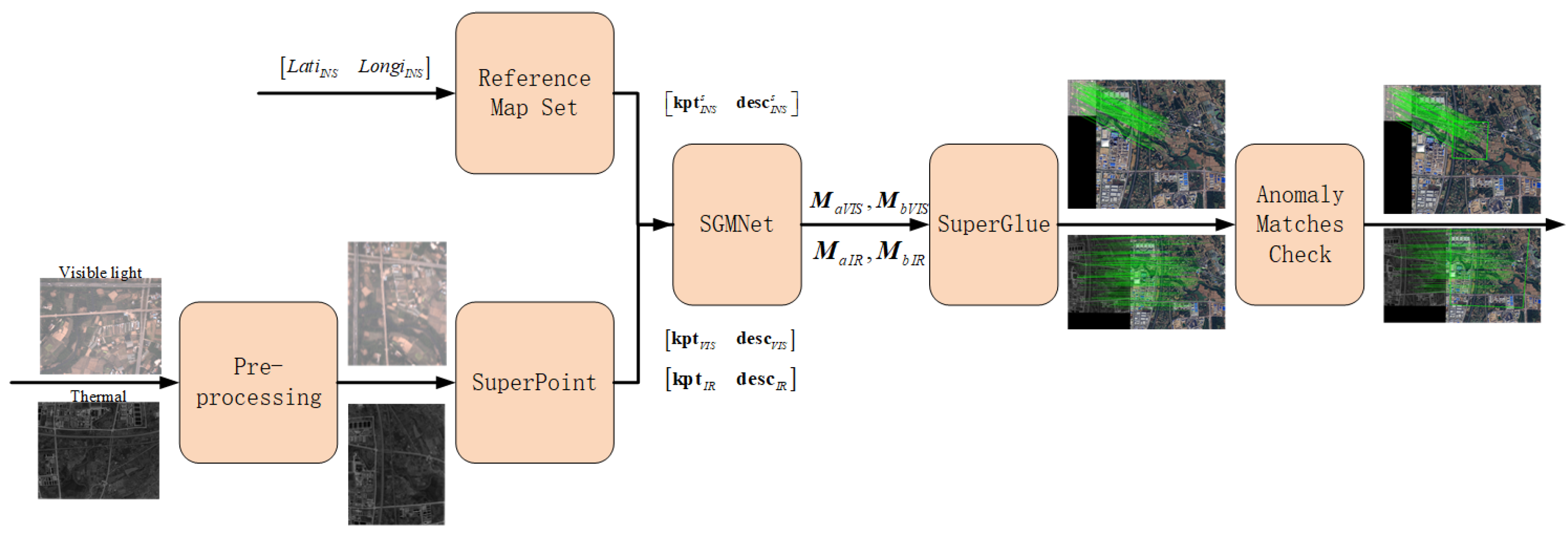
This section presents our visual-inertial navigation system (VINS) framework, which consists of three components: inertial navigation, vision geo-registration, and integrated navigation. The vision geo-registration component matches the camera images (including the visible light and the thermal images) to the reference map and calculates the geolocation of the UAV. The INS component provides high-frequency navigation state and covariance (including attitude, velocity, and position) prediction. The integrated navigation component utilizes vision geo-registration results to compensate for the drift brought by INS prediction. The framework is shown in Figure 2.
3.1. Visual-Inertial System State Construction and Propagation
In this part, we present the filter used in the integrated navigation, including state construction, nominal state propagation, and covariance propagation. We use State Transformation Extend Kalman Filter (ST-EKF) [30,31] to estimate the navigation state.
3.1.1. Nominal State Propagation
In PINS, the nominal state vector can be defined as follows:
where , and are attitude, velocity and position respectively. Note that, in nominal state propagation, the attitude is represented and updated by quaternion , which is different from the filter state outlined below.
, and need to be calculated by using IMU data. Unlike traditional VINS algorithms like VINS-mono and OpenVINS, which use numerical integration to update the state, we use a twin-sample algorithm [32] widely used in inertial navigation to propagate the state.
3.1.2. Filter State
From Section 3.1.1, we can define the error state as:
where , and is attitude error, velocity error, and position error respectively.
Different from the nominal state, in the filter state, we use the Euler angle to represent attitude error.
Then, the linearized error model of INS at time can be described as follows:
where is the noise distribution matrix, and is the noise vector of the system. They are similar to those in traditional Extended Kalman Filter (EKF) of integrated navigation.
The conventional integrated navigation algorithm employing the EKF encounters challenges with inconsistent variance estimation [32]. By reformulating the velocity differential equation, the ST-EKF mitigates the impact of specific force on velocity computation and derives a novel filter system matrix, thereby enhancing the precision of state estimations. According to Reference [30] and [31], the system matrix can be described as follow:
3.1.3. Covariance Propagation
From vision geo-registration that will be presented in Section 3.2 and INS prediction presented in Section 3.1.1, we get a 2D visual localization position and INS prediction position . We define observation , then the observation equation can be described as:
Then, the Jacobi matrix of the observation equation will be:
In covariance propagation, we need to predict the covariance matrix first:
Where is the discretized system matrix, and is the noise distribution covariance matrix.
Then we calculate Kalman gain :
Where is the measurement noise covariance matrix of sensors.
Finally, we update the covariance matrix:
The diagonals of the updated covariance matrix contain elements related to the planimetric position , which will be used to construct the Gaussian elliptic constraint in integrated navigation.
3.2. Cross-Domain Visual Registration
Our work mainly aims at long-duration navigation, which means that the visual geo-localization needs to remain effective at nighttime. This section will present the method how to achieve cross-domain visual registration.
3.2.1. Features Extraction and Matching Method
To achieve day-night vision-based localization, the key is to develop visual features effective on visible light and thermal images. Although a series of hand-craft features and learned features have been used in RGB-image geo-registration [7,8,9,10], few works have shown the capabilities in thermal images.
To obtain a unified feature for cross-domain image matching, we have investigated in multiple hand-craft and learned features, including SIFT [33], XFeat [34], and SuperPoint [35]. Figure 3 shows some samples of the performance of these features on visible light and thermal images. SIFT is applicable to visible light images but demonstrates limited effectiveness on thermal images. XFeat also can be used comparably to SuperPoint in both visible and thermal images, but XFeat exhibits less matching points and matching rate than SuperPoint. The investigation finds that the SuperPoint has shown the best performance in both visible light and thermal matching. In the experimental part, we designed a comparative experiment to prove our conclusion.
3.2.2. Reference Visible Map Pre-Processing
For long-duration navigation, the task areas can be extensive, which brings in difficulties in real-time processing. Therefore, we need to pre-process the reference map before the task to improve the efficiency through the flight.
While the UAVs are equipped with both visible and thermal cameras, we propose only to use remote visible maps for reference, as high-resolution visible maps are easy to obtain.
To improve the algorithm efficiency, we divide the map into submaps and use the predicted location from INS to load the sub-maps. Figure 4 shows the method to build the reference map set.
Firstly, the remote visible light map along the planned flight path needs to be pre-downloaded. Then, we separate the whole map into sub-maps with the size of , which and are actual length of the sub-map in east and north respectively. When the drone flies to the maximum height in the flight, the sub-map should contain as much of the scenery of the camera image as possible. It means:
in which is the maximum height of UAVs, and is the field of view(FOV) of the camera. At the same time, when visual matching localization fails, pure inertial navigation will cause drift. Therefore, it is meaningful to consider appropriately increasing and to avoid map retrieval failure caused by localization divergence, which in turn leads to the complete failure of scene-matching localization. In addition, when the image matching area is close to the edge of the map, matching may fail due to the incomplete matching area. Therefore, when cropping the map, we first crop it to a size of and then stitch adjacent 2x2 map blocks into a sub-map. This ensures that there is a 50% overlap between adjacent sub-maps. Finally, we get the sub-map image set numbered in row and column order.
Then, we build an index of the sub-map set by the latitude and longitude coordinates of the center. Finally, we extract features and descriptors for each sub-map and associate them with the index in Table 1.
3.2.3. Camera Image Pre-Processing
For long-duration tasks, the UAV can fly at different heights and with different headings, which leads to scale and view variations of the camera images. To reduce the visual aliasing between the camera images and the map, image rotation and scaling are applied before geo-registration. Furthermore, for thermal images, we apply gamma transformation to enhance the contrast, thereby highlighting features more and increasing the number of matching pairs.
- Rotation and Scaling
We perform rotation and scaling pre-processing on the images before feature point extraction, to align the geographic coordinate system represented by the images with the reference map (the reference map's default upward direction being north), and to make the pixel resolution close to that of the reference map. The scaling factor can be given by:
Where is relative height, is the pixel resolution of the sub-map, and are camera intrinsics, which can be given by Zhang's camera calibration method [36].
- Thermal Image Gamma Transformation
Infrared imaging is based on the thermal radiation and temperature characteristic differences of ground scenes. However, in high-altitude ground imaging, the collected scenes are mainly large areas of buildings, forests, farmland, roads, etc., with high scene similarity and small thermal radiation differences, leading to infrared imaging having blurred contours, high noises, and low contrast, which is not conducive to feature extraction. Therefore, before extracting features from infrared images, preprocessing of the infrared images can be performed to extract the potential features of the images better. We choose Gamma transformation to adjust image contrast and brightness to enhance details:
In which is the normalized grayscale value of the infrared image, is the grayscale scaling factor, is the gamma value, and is the normalized grayscale value after gamma transformation.
3.2.4. Camera-Map Registration
For visual registration, the key is how to match camera images and reference maps. This part will illustrate the whole process including sub-map querying, registration method and anomaly match checking.
Figure 5.
Camera-map registration.
- Sub-map querying
To achieve camera-map registration, the first step is to search out the corresponding sub-map. In section 3.2.2, the sub-maps are indexed by the 2D geo-position. Therefore, we can query the required sub-map features by position predicted by the INS prediction component.
- Camera-map registration method
SuperGlue [37] is a widely used matching method for SuperPoint features. However, the front end of SuperGlue contains multiple attentions and fully connected networks, which is not conductive in real-time processing. Therefore, we introduce SGMNet [38] to replace this part to improve the efficiency.
When camera image and sub-map features are sent into the SGMNet, the net first calculates two groups of matches and as the seed matches. Then the two seed matches pass through a multiple-layer seed graph network and get the best matches. Finally, the best matches are sent into the back end of SuperGlue to obtain the final matches.
- Anomaly match checking
Because of pre-processing, the matched points of the camera image and map should be connected by lines that are approximately parallel with similar lengths. For incorrect matches, the lines are usually not geometrically close, so it is possible to filter out incorrect matched point pairs by using consistency of the matched point line vectors, thereby removing the inconsistent parts from the set of matched point pairs. Assuming that after matching, there are pairs of matched points in the collection, where the feature point coordinates in the camera image are, and the corresponding feature point coordinates on the sub-map are. Then, the line vector for each set of matched point pairs is:
For each , we can calculate its magnitude and slope:
We define the distance consistency threshold and direction consistency threshold , and then we can get consistency set for each :
At this point, if the number of filtered matches does not meet the threshold of a successful registration, it is considered a failed registration, thereby eliminating incorrectly matched images. If the number of matches meets the threshold, the obtained matches should have eliminated the vast majority of incorrect matches.
3.3. Geo-Localization from Visual Registration
After matching, we get a set of matching point pairs. In this part, we illustrate the method for obtaining location from visual registration to get the visual geo-localization result. Furthermore, we consider the influence of attitude in geo-localization and the design compensation method.
3.3.1. Geo-Localization
The matching relationship between images can be modeled as an affine transformation. Consequently, in our approach, the geo-location of any point on the reference map within the images taken from UAV can be determined by computing the affine transformation matrix . We use homography matrix estimation based on Random Sample Consensus (RANSAC) to determine the affine matrix. If we assume that the center of the camera image is the location of the UAV, we can transform the camera image into the reference map by using . We will get the transformed center of the camera image , and the center of the reference map represents the location in the real world . Then the location of the UAV can be given by:
where is the pixel resolution of a map (length in the world coordinate system represented by a single pixel, with units in meters per pixel (m/pix).
3.3.2. Horizontal Attitude Error Compensation
In this part, we use the NED(north-east-down) local geodetic coordinate frame as the navigation coordinate frame(n-frame) and the FRD(front-right-down) frame as the carrier coordinate frame(b-frame). Then we can define rotation matrixes:
We can define a unit vector in the n-system. Then we can transform the vector to the body frame as:
Where , and are roll, pitch, and yaw respectively.
Next, the transformed unit vector can be expressed in spherical coordinates like Figure 6, where
Finally, the eastward error and northward error can be given by:
Where is the relative height of UAV.
3.4. Filter State Updation with GeoLocalization Observations
We use the above methods to ensure the correctness of geo-localization as much as possible. Despite this, geo-localization results will inevitably contain some wrong localization consequences. To eliminate these inaccuracy results, we introduce Gaussian elliptic constraint [39] to inspect the availability of visual geo-localization before ST-EKF.
Figure 7.
Gaussian elliptic constraint. The Gaussian ellipse is constructed by , and filter only accepts visual geo-localization position amidst the ellipse as the observation.
Figure 7.
Gaussian elliptic constraint. The Gaussian ellipse is constructed by , and filter only accepts visual geo-localization position amidst the ellipse as the observation.
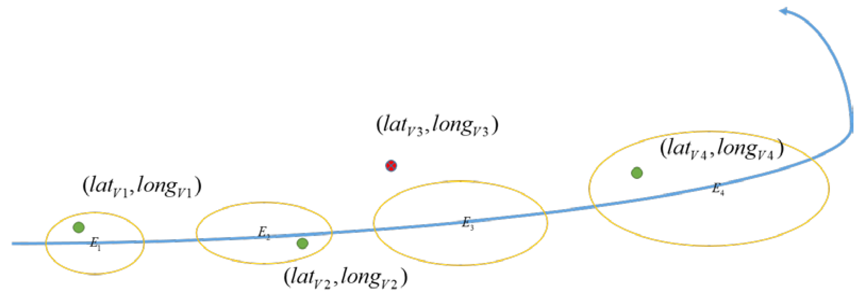
In ST-EKF, the diagonal elements of the covariance matrix represent the error bounds of each state variable. Then we can use planar position-related elements and in to establish a Gaussian elliptic equation:
If does not satisfy the Gaussian elliptic constraint, this observation will not be used in integrated navigation.
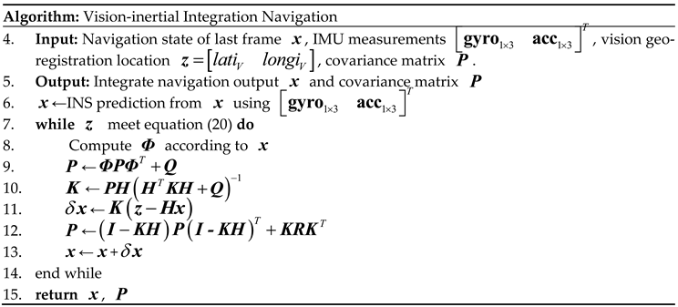
The pseudocode of state updating is as follows:

Table 2.
Pseudocode of state updating.
4. Experiment
To prove the effectiveness of the proposed method, we designed a set of experiments, including a comparison of feature matching between several different features, a vision geo-localization experiment and an integrated navigation experiment.
4.1. System Setup
The experiment location was in Jinmen, Hubei. We used a CH-4 UAV as the carrier, and the experiment system includes a Laser IMU working at 200Hz, a set of down-looking- cameras that consist of a visual light camera and an infrared camera, a barometric altimeter, and a satellite receiver that can output differential GPS data as the ground truth. The experiment was in a area as Figure 8(a). Figure 8(b) shows the UAV and camera set. And Table 3 shows some parameters of cameras.
4.2. Dataset Description and Evaluation Method
Two datasets were used to test the proposed method. Dataset 1 was collected in May. 22nd, 2024, which includes daytime and nighttime RGB and thermal camera images. Dataset 2 was obtained in May. 9th, 2024; this dataset only has visible light images. The details of the two datasets are shown in Table 4.
Table 4.
Experiment datasets.
| Dataset | Dataset 1 | Dataset 2 |
|---|---|---|
| Cruising Altitude(m) | 2400 | 700 |
| Time(s) | 6892 | 5170 |
| Length(km) | 344.6 | 284.35 |
| Daytime(s) | 2504 | 5170 |
| Frequency(Hz) | 1 | 1 |
| Acceptable Matching Threshold | 50 | 50 |
| Location Error Threshold(m) | 100 | 100 |
Based on the two datasets, three groups of experiments were conducted. The first experiment is feature matching. There are three features used in the experiment, SIFT , XFeat and SuperPoint. In the experiment, we choose 50 matches as the threshold of an acceptable visual registration and define the matching rate as the proportion of the accepted visual registrations in the dataset. In addition, both visible light and thermal images are registered with a visible light map.
The second experiment is the geo-localization experiment. We use SuperPoint features to match images and evaluate precision by root mean square error (RMSE) in experiments. We set 100 meters as the threshold of a valid geo-localization result. Like the definition of matching rate, we define valid matching rate as the proportion of the valid geo-localization in the dataset. Besides, we compare the accuracy and number of effective geo-localizations with or without attitude compensation to verify the effectiveness of attitude compensation.
The last experiment is the integrated navigation experiment. Since IMU data is only available in Dataset 2, we use a single Dataset 2 for the integrated navigation experiment. We prove the effectiveness of the proposed algorithm by comparing errors with or without proposed filtering methods.
4.3. Experimental Results
4.3.1. Registration Rate Results
This experiment presents the matching rate of three features in the two datasets, SIFT, XFeat, and SuperPoint. Figure 9 and Figure 10 show the performance of the three features in Dataset 1 and Dataset 2 respectively,
The matching rate of SIFT on both visible light and thermal images is far less than XFeat and SuperPoint. On visible light images, XFeat achieves a matching rate of 31.14%, close to 32.72% of SuperPoint. However, when applied to thermal images, XFeat exhibits inferior performance compared to SuperPoint. The performance of SuperPoint on infrared images is the best among the three features, with a matching rate of 68.67%. Considering the effectiveness of registration, the effective matching rate of SIFT on visible light images is only 2.9%, and only two images exhibit linear errors of less than 100 meters. Although XFeat maintained a satisfactory localization precision in visible light, its performance in thermal images remained suboptimal. SuperPoint has the best performance in localization, with an effective matching rate of 22.47% in visible light and 54.03% in thermal.
Additionally, from Figure 9, it can be concluded that while the geo-localization rate of visible images is superior to that of thermal images, thermal images can address the limitation of visible images being unusable at nighttime.
Figure 9.
Matching rate and effective matching rate in Dataset 1. SuperPoint has the best performance of the three features in both registration and localization. Visible light images are easy to register and locate but thermal images can register and locate in nighttime.
Figure 9.
Matching rate and effective matching rate in Dataset 1. SuperPoint has the best performance of the three features in both registration and localization. Visible light images are easy to register and locate but thermal images can register and locate in nighttime.
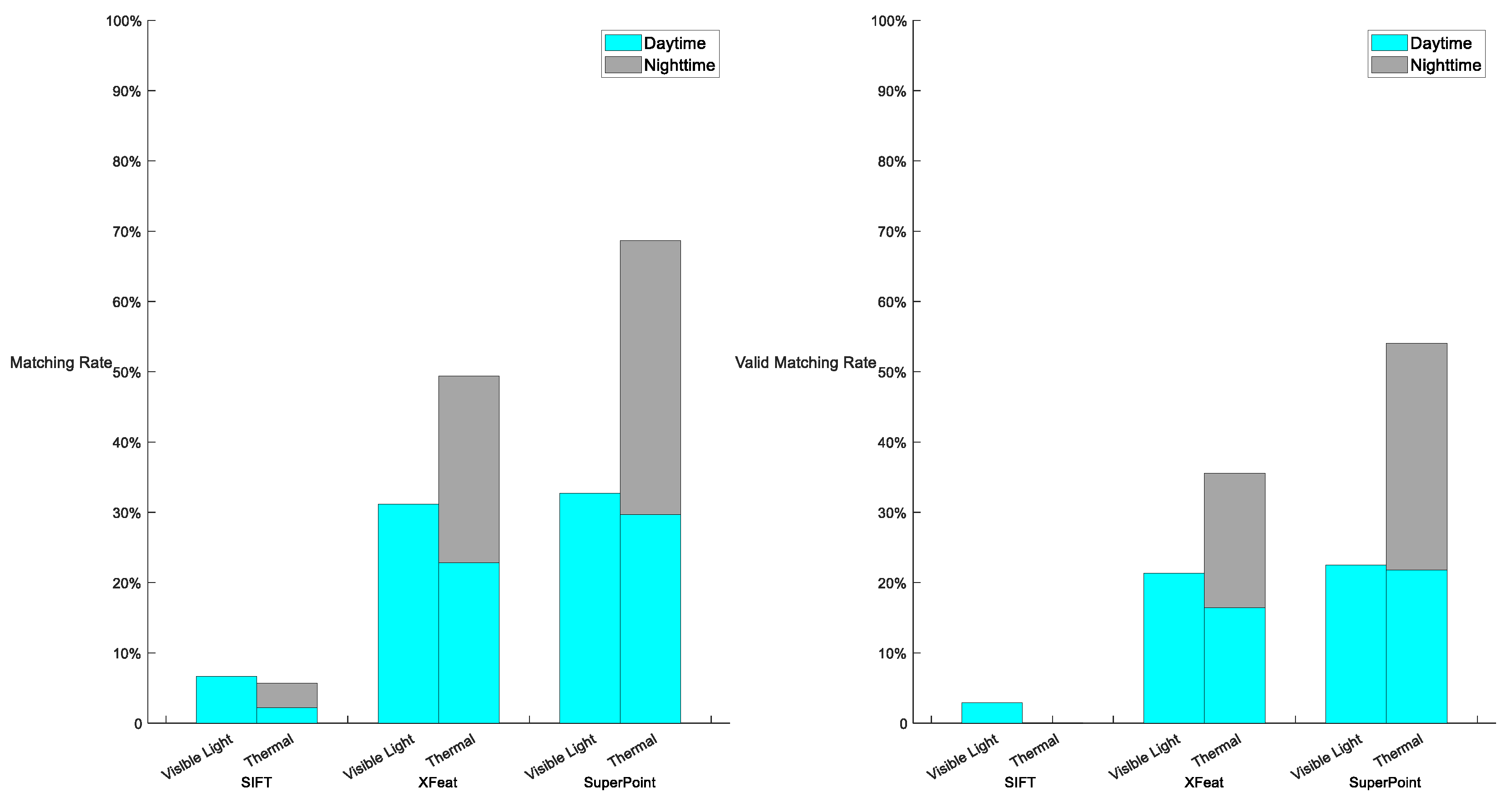
Figure 10.
Performance of three features in Dataset 2.
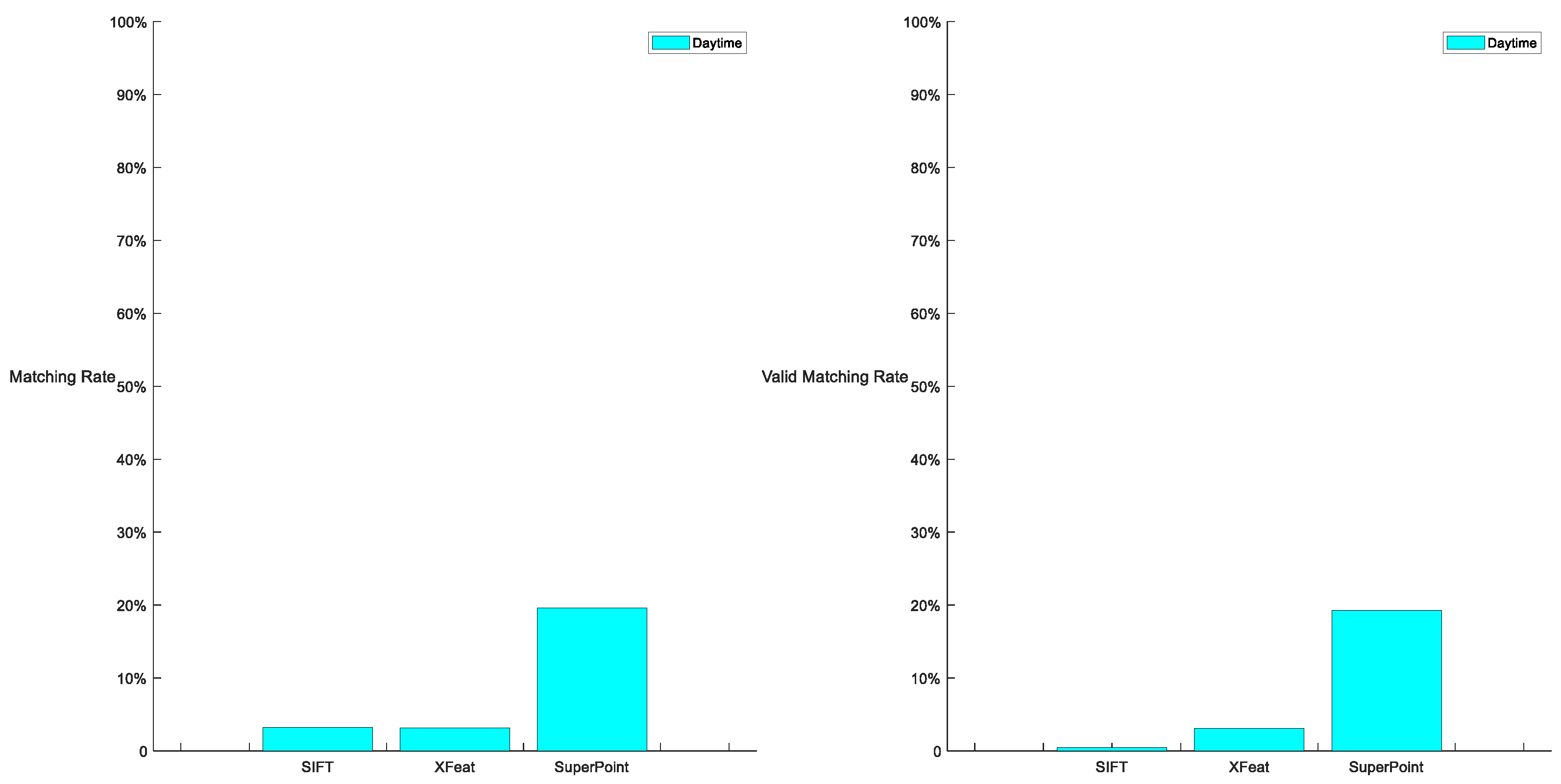
The results of the three features on Dataset 2 exhibit performance consistent with the aforementioned analysis. Note that, the matching rate in Dataset 2 is lower than that in Dataset 1. It is because that the cruising altitude of Dataset 2 is lower than that of Dataset 1. It means that images of Dataset 2 have a smaller FOV than Dataset 1. This indicates that images from Dataset 2 contain fewer distinctive features for extraction, consequently leading to a lower matching rate. Additionally, as a lightweight model, XFeat demonstrates greater degradation than SuperPoint in matching performance due to FOV contraction and the reduced availability of features. The sample images of XFeat in Section 3.2.4 also demonstrate similar conclusions.
4.3.2. Visual Geo-Localization Results
This experiment mainly presents the efficiency of attitude compensation. We use RMSE to describe the precision of geo-localization.
We evaluate the RMSE of geo-localization above in Figure 11. The figure shows that attitude compensation can improve the precision of geo-localization. In addition, after attitude compensation, the visible light geo-localization shows better precision than thermal. At last, by comparing the precision between Dataset 1 and Dataset 2, we can discover that different heights can influence the precision of geo-localization. The reason is that according to the equation (11), the pixel resolution of the map and relative height will affect the scaling factor. If the scaling factor is excessively small, it will be difficult to extract enough features used in registration, which leads to a worse matching rate. Therefore, for better registration performance, we try to control the scaling factor between 0.5 and 1. It means that we should confirm flight altitude and choose the map with the corresponding pixel resolution before the flight.
Figure 12 presents sample images of visible light and thermal which attitude compensation has effect on. We can easily see that both samples perform well in registration, but the geo-localization results show a large error. It illustrates that the horizontal attitude angle significantly impacts the visual geo-localization as the UAV approaches the turning point. In our experiment, the UAV consistently operates at a specified altitude. Therefore, the experimental data only clearly indicate that the roll angle significantly influences the geo-localization precision.
4.3.3. Visual-Inertial Integrated Navigation Results
We use Dataset 2 to present the effectiveness of our VINS method. Figure 13 shows the trajectory of integrated navigation.
The experiment lasted 5170 seconds. From section 4.3.1, we know that there are 997 correct matches. In integrated navigation, 1007 matches are used in ST-EKF, which proves that the proposed attitude compensation and Gaussian elliptic constraint can improve the availability of vision geo-registration.
We use GPS and INS integrated navigation as the ground truth, and compare VINS results with and without Gaussian elliptic constraint. We evaluate the precision using root mean square error (RMSE).
Table 5 shows the precision statistics of the experiment. When using integrated navigation without Gaussian elliptic constraint, the RMSE is 112.65 meters. But the RMSE of the proposed method is 42.38 meters. As demonstrated by Figure 13 and Table 5, the Gaussian elliptic constraint identified and excluded five outliers. These high-error points, if incorporated into the EKF, would significantly compromise the precision of integrated navigation solutions. This experimental result statistically corroborates the efficacy of our proposed Gaussian elliptic constraint methodology.
Figure 14 shows some sample matches eliminated by Gaussian elliptic constraint. Most eliminated matches occur in environments characterized by more repetitive and homogeneous terrain. Visual registration cannot hold robust in these environments, and registration results will be either that there are too few features to match, or that the matching result is to match the terrain similar to the real position, resulting in localization error like Figure 14. From the trajectory, we can see that the variety of mismatches has negative effect on ST-EKF, but these mismatches are difficult to eliminate by simply visual strategies. Gaussian elliptic constraint can eliminate them by using the covariance matrix of ST-EKF, and leave more accurate observations for the integrated navigation system.
5. Conclusions
In this paper, we establish a VINS framework to solve long-term navigation problems in GNSS-denied situations. The framework consists of vision registration, INS prediction, and ST-EKF, which uses vision geo-registration to redress the PINS error. We analyze the influence of attitude on vision geo-localization and propose a compensation method to increase the precision of visual geo-localization. The proposed method makes ST-EKF get more observations with fewer position errors in GNSS-denied situations. The designed experiment proves the effectiveness of our method.
From the experiment, we find that in mountain scenes or other scenes that have high repeatability, the vision geo-registration does not work well. So how to increase visual navigation in these situations may be the next direction of our research.
Author Contributions
Conceptualization, Xuehui Xing and Xiaofeng He; Data curation, Xuehui Xing; Formal analysis, Xuehui Xing; Methodology, Xuehui Xing and Ke Liu; Project administration, Jun Mao; Resources, Xiaofeng He, Lilian Zhang, and Jun Mao; Software, Xuehui Xing, Ke Liu, Zhizhong Chen, Guofeng Song and Qikai Hao; Supervision, Xiaofeng He, Lilian Zhang and Jun Mao; Validation, Xuehui Xing; Visualization, Xuehui Xing; Writing – original draft, Xuehui Xing, Xiaofeng He and Ke Liu; Writing – review & editing, Lilian Zhang and Jun Mao.
Funding
This research was funded by the National Nature Science Foundation of China, grant number 62103430, 62103427 and 62073331.
References
- Couturier, A.; Akhloufi, M.A. A review on absolute visual localization for UAV. Robotics and Autonomous Systems 2021, 135, 103666. [Google Scholar] [CrossRef]
- Fraundorfer, F.; Scaramuzza, D. Visual odometry: Part i: The first 30 years and fundamentals. IEEE Robotics and Automation Magazine 2011, 18, 80–92. [Google Scholar]
- Scaramuzza, D.; Zhang, Z. Visual-inertial odometry of aerial robots. arXiv 2019, arXiv:1906.03289. [Google Scholar]
- Qin, T.; Li, P.; Shen, S. Vins-mono: A robust and versatile monocular visual-inertial state estimator. IEEE transactions on robotics 2018, 34, 1004–1020. [Google Scholar] [CrossRef]
- Campos, C.; Elvira, R.; Rodríguez, J.J.G.; Montiel, J.M.; Tardós, J.D. Orb-slam3: An accurate open-source library for visual, visual–inertial, and multimap slam. IEEE Transactions on Robotics 2021, 37, 1874–1890. [Google Scholar] [CrossRef]
- Geneva, P.; Eckenhoff, K.; Lee, W.; Yang, Y.; Huang, G. Openvins: A research platform for visual-inertial estimation. In Proceedings of the 2020 IEEE International Conference on Robotics and Automation (ICRA); 2020; pp. 4666–4672. [Google Scholar]
- Bianchi, M.; Barfoot, T.D. UAV localization using autoencoded satellite images. IEEE Robotics and Automation Letters 2021, 6, 1761–1768. [Google Scholar] [CrossRef]
- Patel, B.; Barfoot, T.D.; Schoellig, A.P. Visual localization with google earth images for robust global pose estimation of uavs. In Proceedings of the 2020 IEEE international conference on robotics and automation (ICRA); 2020; pp. 6491–6497. [Google Scholar]
- Conte, G.; Doherty, P. Vision-based unmanned aerial vehicle navigation using geo-referenced information. EURASIP Journal on Advances in Signal Processing 2009, 2009, 1–18. [Google Scholar] [CrossRef]
- Mantelli, M.; Pittol, D.; Neuland, R.; Ribacki, A.; Maffei, R.; Jorge, V.; Prestes, E.; Kolberg, M. A novel measurement model based on abBRIEF for global localization of a UAV over satellite images. Robotics and Autonomous Systems 2019, 112, 304–319. [Google Scholar] [CrossRef]
- Jiang, X.; Ma, J.; Xiao, G.; Shao, Z.; Guo, X. A review of multimodal image matching: Methods and applications. Information Fusion 2021, 73, 22–71. [Google Scholar] [CrossRef]
- Dwith Chenna, Y.N.; Ghassemi, P.; Pfefer, T.J.; Casamento, J.; Wang, Q. Free-form deformation approach for registration of visible and infrared facial images in fever screening. Sensors 2018, 18, 125. [Google Scholar] [CrossRef] [PubMed]
- Yu, K.; Ma, J.; Hu, F.; Ma, T.; Quan, S.; Fang, B. A grayscale weight with window algorithm for infrared and visible image registration. Infrared Physics & Technology 2019, 99, 178–186. [Google Scholar]
- Hrkać, T.; Kalafatić, Z.; Krapac, J. Infrared-visual image registration based on corners and hausdorff distance. In Proceedings of the Image Analysis: 15th Scandinavian Conference, SCIA 2007, Aalborg, Denmark, 10-14 June 2007; pp. 383–392. [Google Scholar]
- Ma, J.; Zhao, J.; Ma, Y.; Tian, J. Non-rigid visible and infrared face registration via regularized Gaussian fields criterion. Pattern Recognition 2015, 48, 772–784. [Google Scholar] [CrossRef]
- Du, Q.; Fan, A.; Ma, Y.; Fan, F.; Huang, J.; Mei, X. Infrared and visible image registration based on scale-invariant piifd feature and locality preserving matching. IEEE Access 2018, 6, 64107–64121. [Google Scholar] [CrossRef]
- Zeng, Q.; Adu, J.; Liu, J.; Yang, J.; Xu, Y.; Gong, M. Real-time adaptive visible and infrared image registration based on morphological gradient and C_SIFT. Journal of Real-Time Image Processing 2020, 17, 1103–1115. [Google Scholar] [CrossRef]
- Forster, C.; Zhang, Z.; Gassner, M.; Werlberger, M.; Scaramuzza, D. SVO: Semidirect visual odometry for monocular and multicamera systems. IEEE Transactions on Robotics 2016, 33, 249–265. [Google Scholar] [CrossRef]
- Engel, J.; Koltun, V.; Cremers, D. Direct sparse odometry. IEEE transactions on pattern analysis and machine intelligence 2017, 40, 611–625. [Google Scholar] [CrossRef] [PubMed]
- Mur-Artal, R.; Montiel, J.M.M.; Tardos, J.D. ORB-SLAM: a versatile and accurate monocular SLAM system. IEEE transactions on robotics 2015, 31, 1147–1163. [Google Scholar] [CrossRef]
- Van Dalen, G.J.; Magree, D.P.; Johnson, E.N. Absolute localization using image alignment and particle filtering. In Proceedings of the AIAA Guidance, Navigation, and Control Conference; 2016; p. 0647. [Google Scholar]
- Yol, A.; Delabarre, B.; Dame, A.; Dartois, J.-E.; Marchand, E. Vision-based absolute localization for unmanned aerial vehicles. In Proceedings of the 2014 IEEE/RSJ International Conference on Intelligent Robots and Systems; 2014; pp. 3429–3434. [Google Scholar]
- Conte, G.; Doherty, P. An integrated UAV navigation system based on aerial image matching. In Proceedings of the 2008 IEEE Aerospace Conference; 2008; pp. 1–10. [Google Scholar]
- Calonder, M.; Lepetit, V.; Strecha, C.; Fua, P. Brief: Binary robust independent elementary features. In Proceedings of the Computer Vision–ECCV 2010: 11th European Conference on Computer Vision, Heraklion, Crete, Greece, September 5-11, 2010, Proceedings, Part IV 11, 2010; pp. 778–792.
- Surber, J.; Teixeira, L.; Chli, M. Robust visual-inertial localization with weak GPS priors for repetitive UAV flights. In Proceedings of the 2017 IEEE International Conference on Robotics and Automation (ICRA); 2017; pp. 6300–6306. [Google Scholar]
- Shan, M.; Wang, F.; Lin, F.; Gao, Z.; Tang, Y.Z.; Chen, B.M. Google map aided visual navigation for UAVs in GPS-denied environment. In Proceedings of the 2015 IEEE international conference on robotics and biomimetics (ROBIO); 2015; pp. 114–119. [Google Scholar]
- Nassar, A.; Amer, K.; ElHakim, R.; ElHelw, M. A deep CNN-based framework for enhanced aerial imagery registration with applications to UAV geolocalization. In Proceedings of the Proceedings of the IEEE conference on computer vision and pattern recognition workshops, 2018; pp. 1513–1523.
- Wang, L.; Gao, C.; Zhao, Y.; Song, T.; Feng, Q. Infrared and visible image registration using transformer adversarial network. In Proceedings of the 2018 25th IEEE International Conference on Image Processing (ICIP); 2018; pp. 1248–1252. [Google Scholar]
- Baruch, E.B.; Keller, Y. Multimodal matching using a hybrid convolutional neural network. Ben-Gurion University of the Negev, 2018.
- Wang, M.; Wu, W.; He, X.; Li, Y.; Pan, X. Consistent ST-EKF for long distance land vehicle navigation based on SINS/OD integration. IEEE Transactions on Vehicular Technology 2019, 68, 10525–10534. [Google Scholar] [CrossRef]
- Wang, M.; Wu, W.; Zhou, P.; He, X. State transformation extended Kalman filter for GPS/SINS tightly coupled integration. Gps Solutions 2018, 22, 1–12. [Google Scholar] [CrossRef]
- Robert, E.; Perrot, T. Invariant filtering versus other robust filtering methods applied to integrated navigation. In Proceedings of the 2017 24th Saint Petersburg International Conference on Integrated Navigation Systems (ICINS); 2017; pp. 1–7. [Google Scholar]
- Ng, P.C.; Henikoff, S. SIFT: Predicting amino acid changes that affect protein function. Nucleic acids research 2003, 31, 3812–3814. [Google Scholar] [CrossRef] [PubMed]
- Potje, G.; Cadar, F.; Araujo, A.; Martins, R.; Nascimento, E.R. XFeat: Accelerated Features for Lightweight Image Matching. In Proceedings of the Proceedings of the IEEE/CVF Conference on Computer Vision and Pattern Recognition, 2024; pp. 2682–2691.
- DeTone, D.; Malisiewicz, T.; Rabinovich, A. Superpoint: Self-supervised interest point detection and description. In Proceedings of the Proceedings of the IEEE conference on computer vision and pattern recognition workshops, 2018; pp. 224–236.
- Zhang, Z. Flexible camera calibration by viewing a plane from unknown orientations. In Proceedings of the Proceedings of the seventh ieee international conference on computer vision, 1999; pp. 666–673.
- Sarlin, P.-E.; DeTone, D.; Malisiewicz, T.; Rabinovich, A. Superglue: Learning feature matching with graph neural networks. In Proceedings of the Proceedings of the IEEE/CVF conference on computer vision and pattern recognition, 2020; pp. 4938–4947.
- Chen, H.; Luo, Z.; Zhang, J.; Zhou, L.; Bai, X.; Hu, Z.; Tai, C.-L.; Quan, L. Learning to match features with seeded graph matching network. In Proceedings of the Proceedings of the IEEE/CVF international conference on computer vision, 2021; pp. 6301–6310.
- Liu, K.; He, X.; Mao, J.; Zhang, L.; Zhou, W.; Qu, H.; Luo, K. Map Aided Visual-Inertial Integrated Navigation for Long Range UAVs. In Proceedings of the International Conference on Guidance, Navigation and Control, 2022; pp. 6043–6052.
Figure 1.
The reference map set is built offline. The UAV obtains visible light and thermal images by camera set and calculates visual position through visual geo-localization online. Then, UAV uses the attitude predicted by INS to compensate for errors. Finally, visual geo-localization results and predicting navigation state are fused to acquire the integrated navigation parameters.
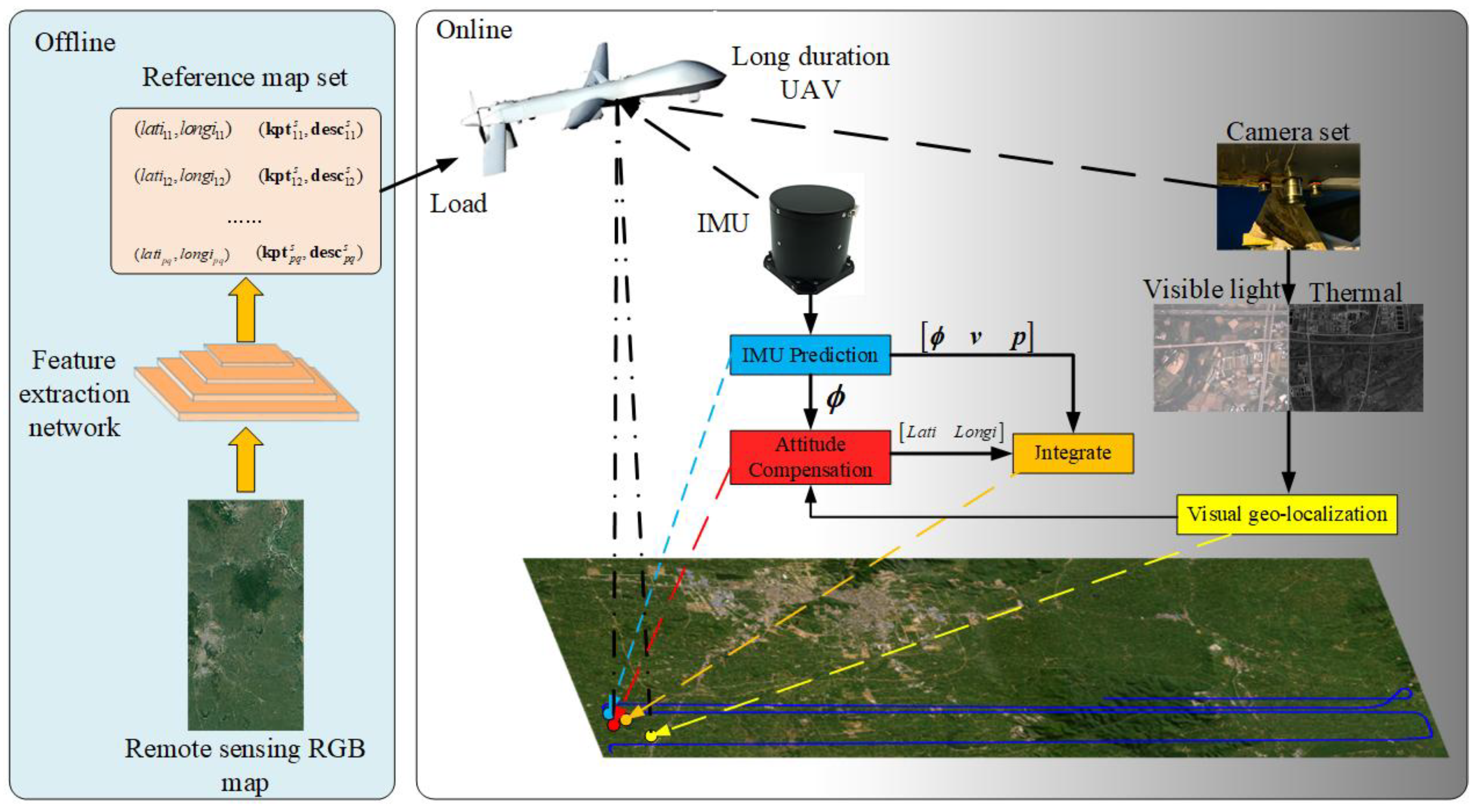
Figure 2.
VINS Framework. IMU provides measurements for INS prediction and gets pure inertial navigation system(PINS) navigation parameters. The camera set offers visible light and thermal camera images to vision geo-registration, and localization results are calculated. Then PINS result and visual result are integrated by ST-EKF.
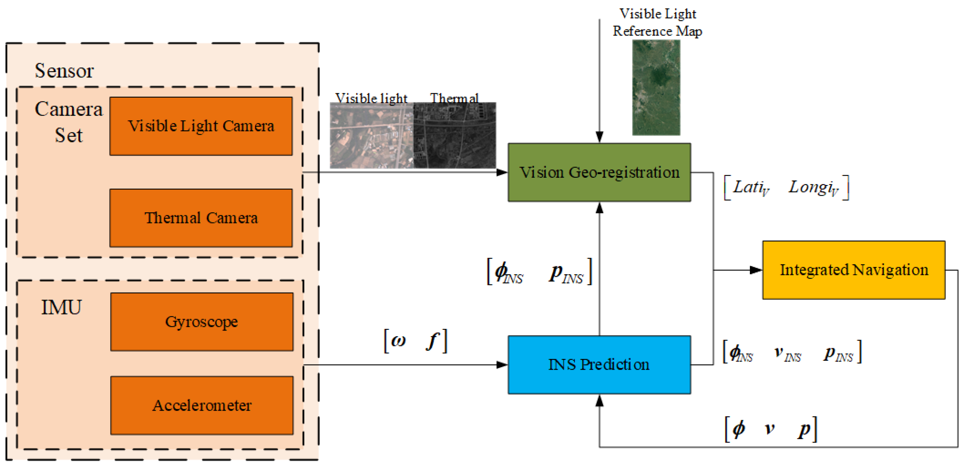
Figure 3.
Sample images of three features performing on visible light and thermal images.
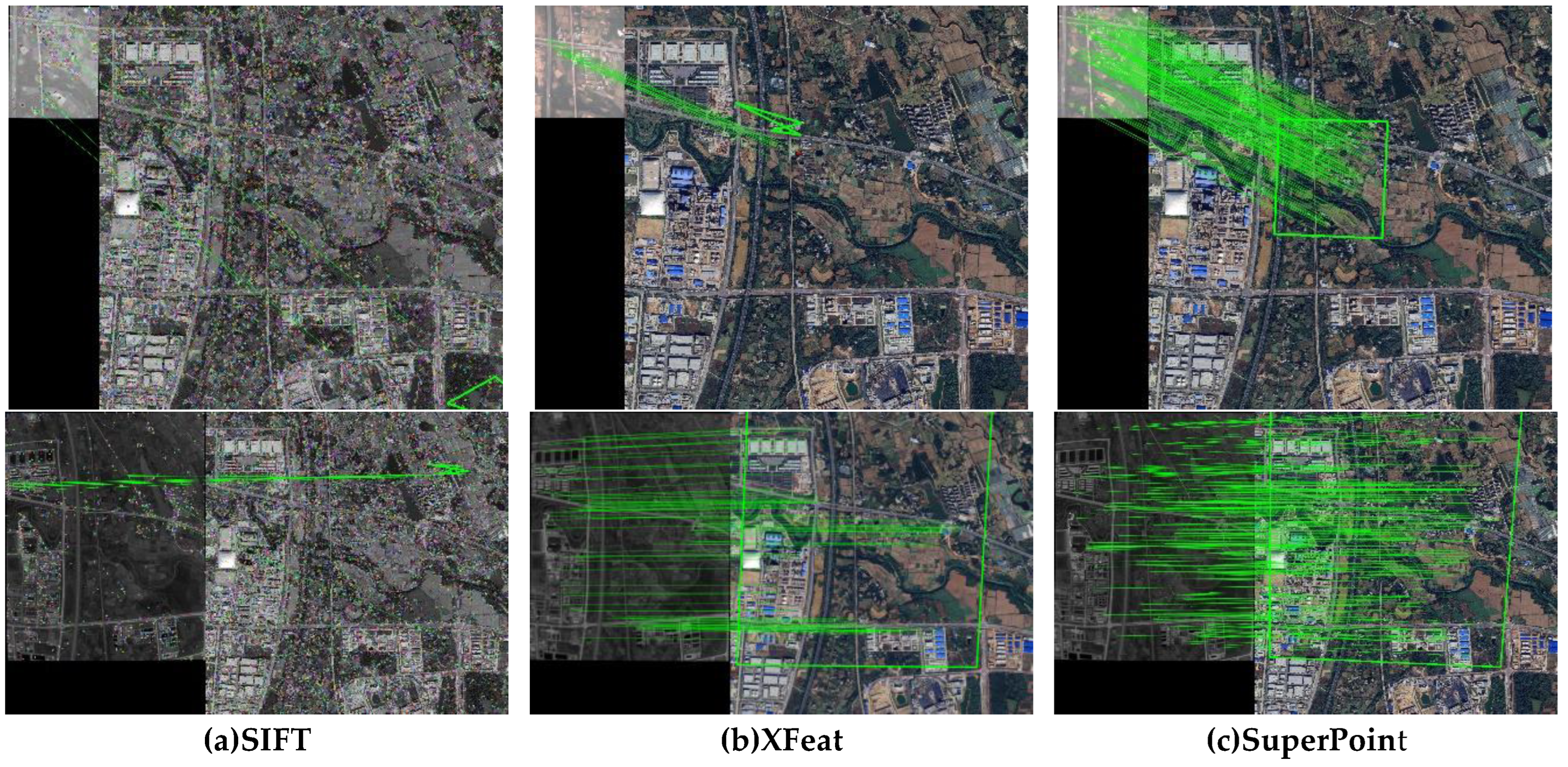
Figure 4.
Building reference map set.
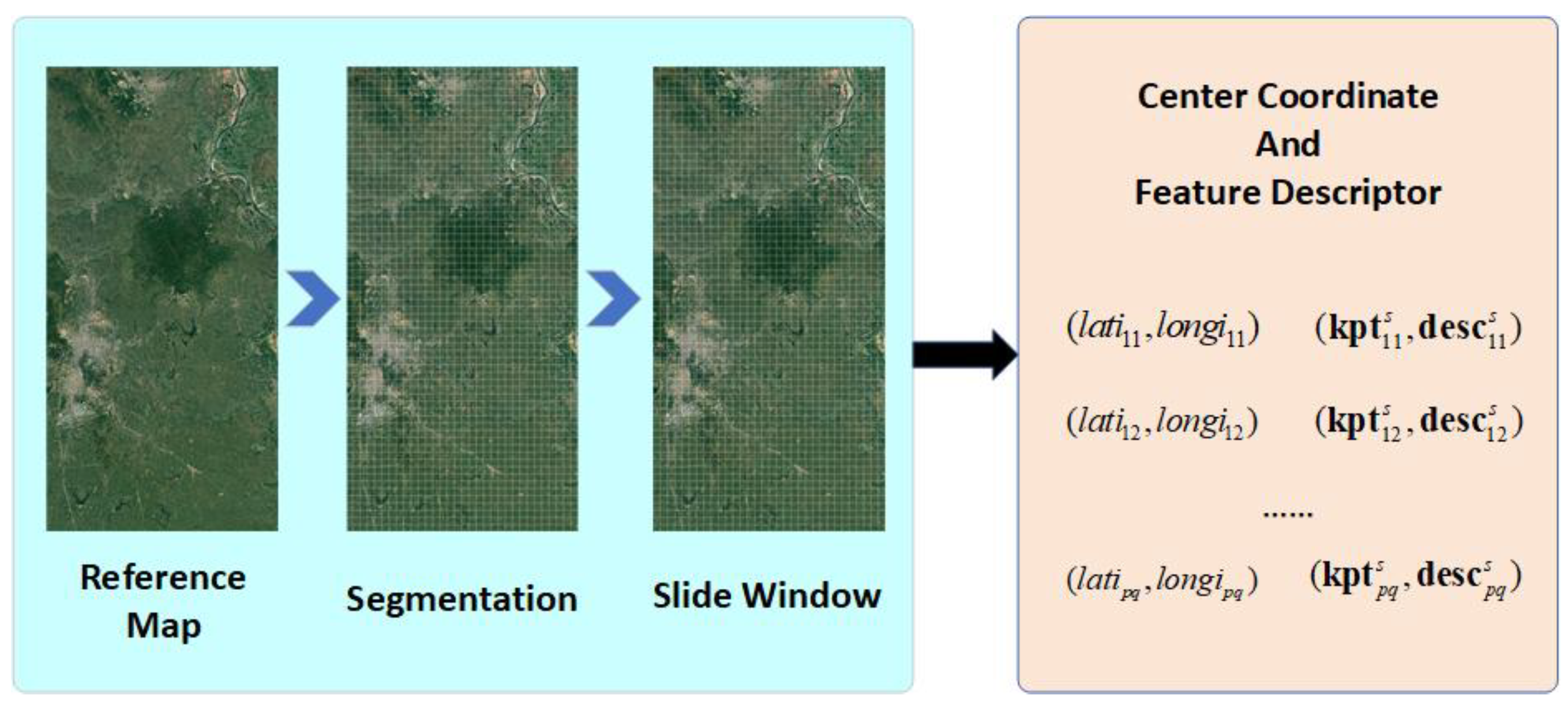
Figure 6.
Spherical Coordinate System.
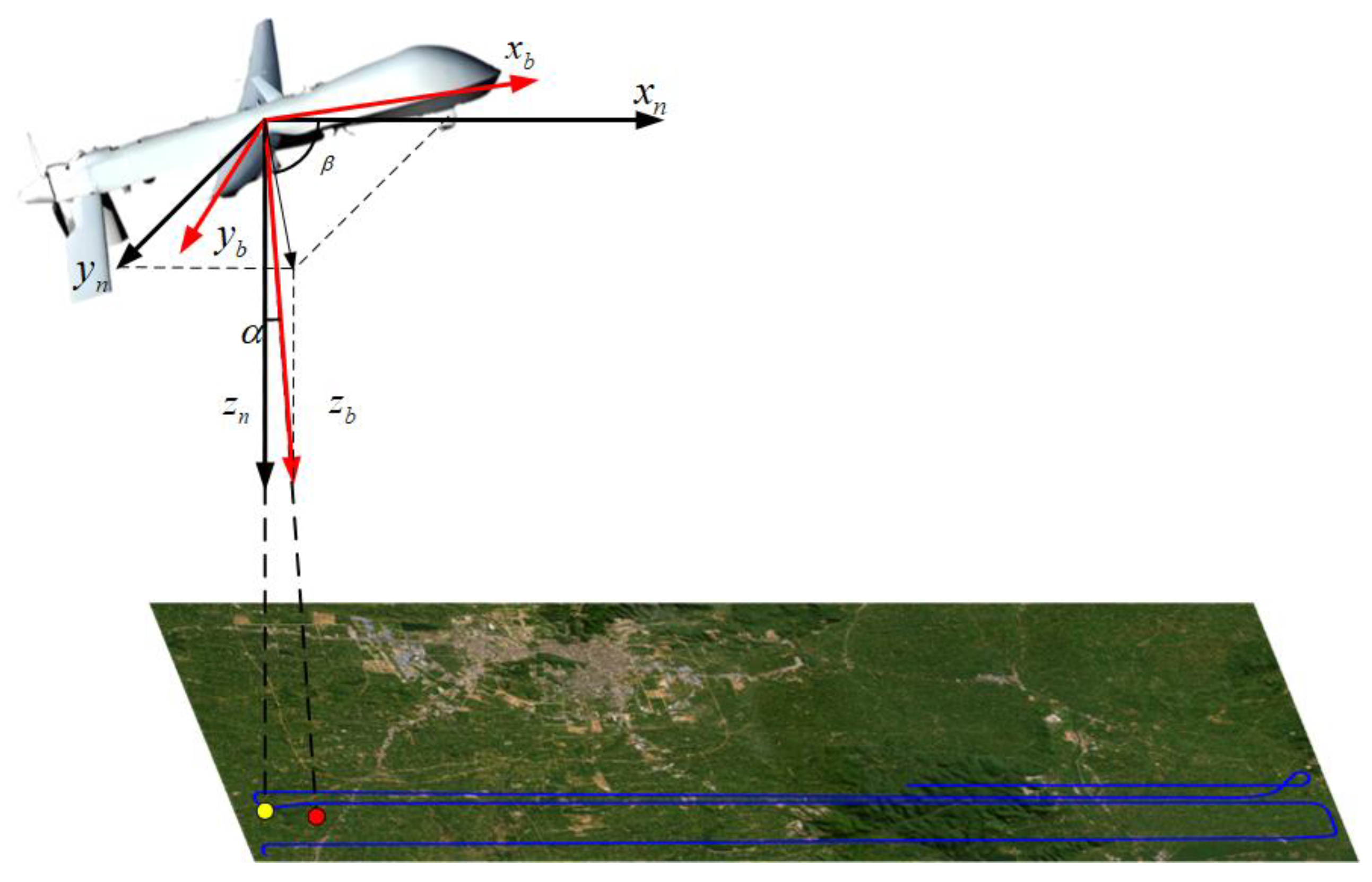
Figure 8.
Experiment conditions.
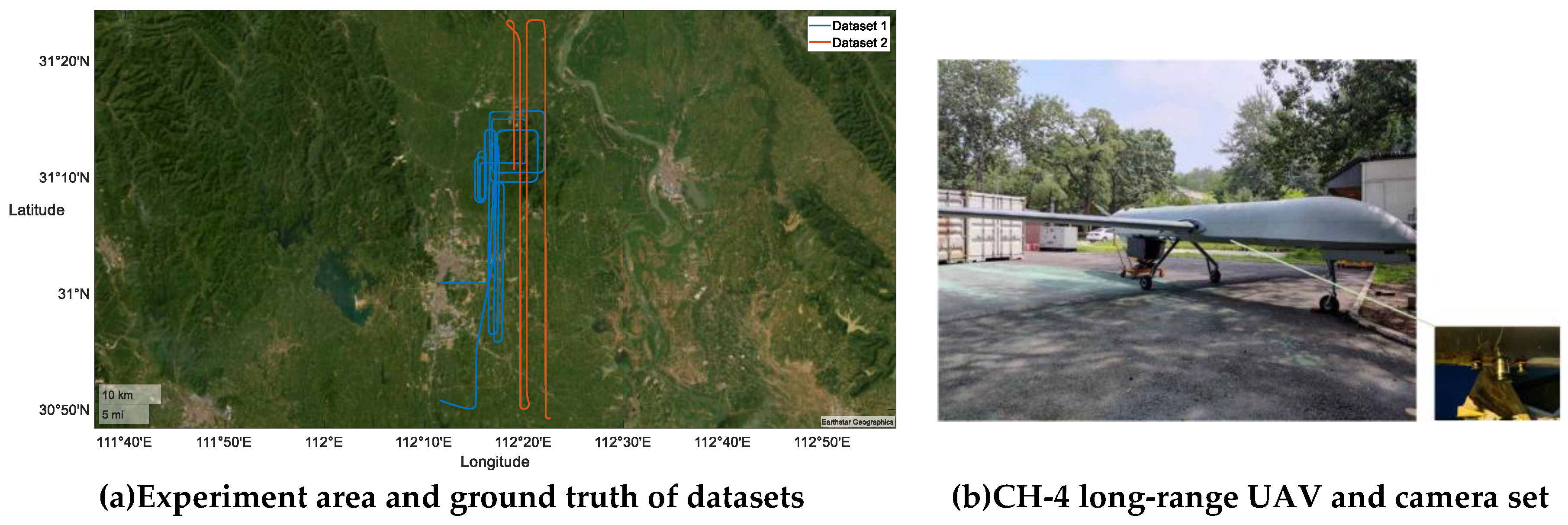
Figure 11.
RMSE of geo-localization. With attitude compensation, RMSE of both datasets is smaller than that without attitude compensation. Visible light images have higher matching rate but have larger RMSE before attitude compensation. After attitude compensation, visible light images have better performance than thermal. Dataset 2 has lower height than Dataset 1, which has lower RMSE and matching rate.
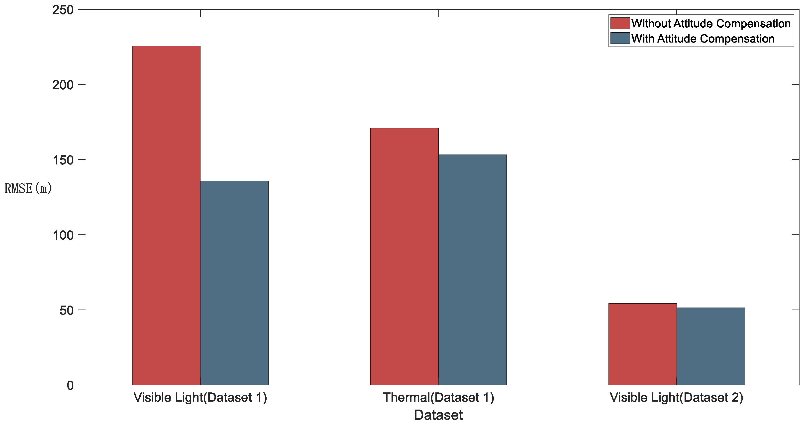
Figure 12.
Visible light and thermal sample of attitude compensation.
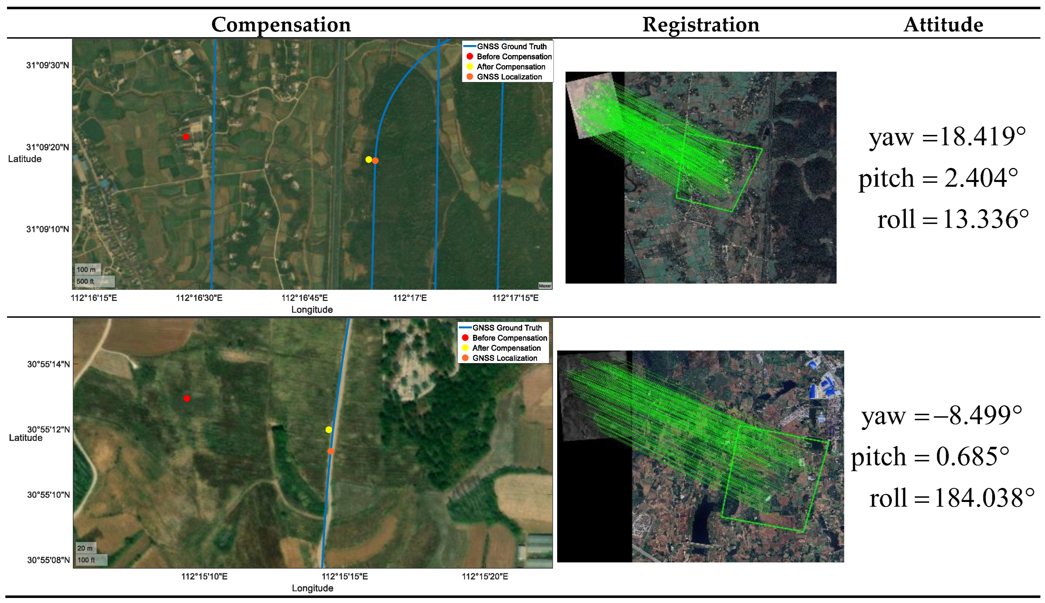
Figure 13.
Integrated navigation trajectory.
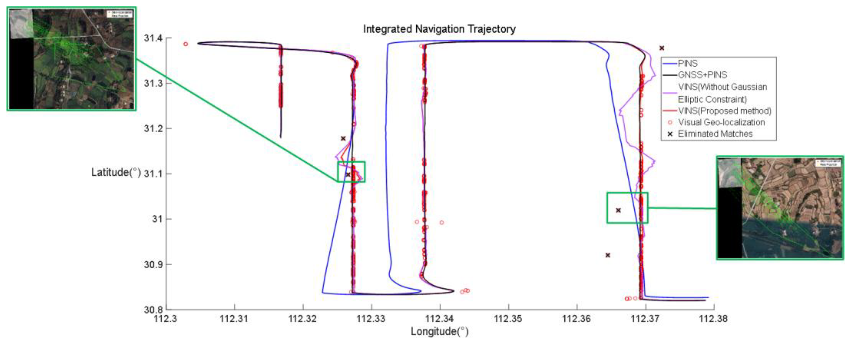
Figure 14.
Matches eliminated by Gaussian elliptic constraint.
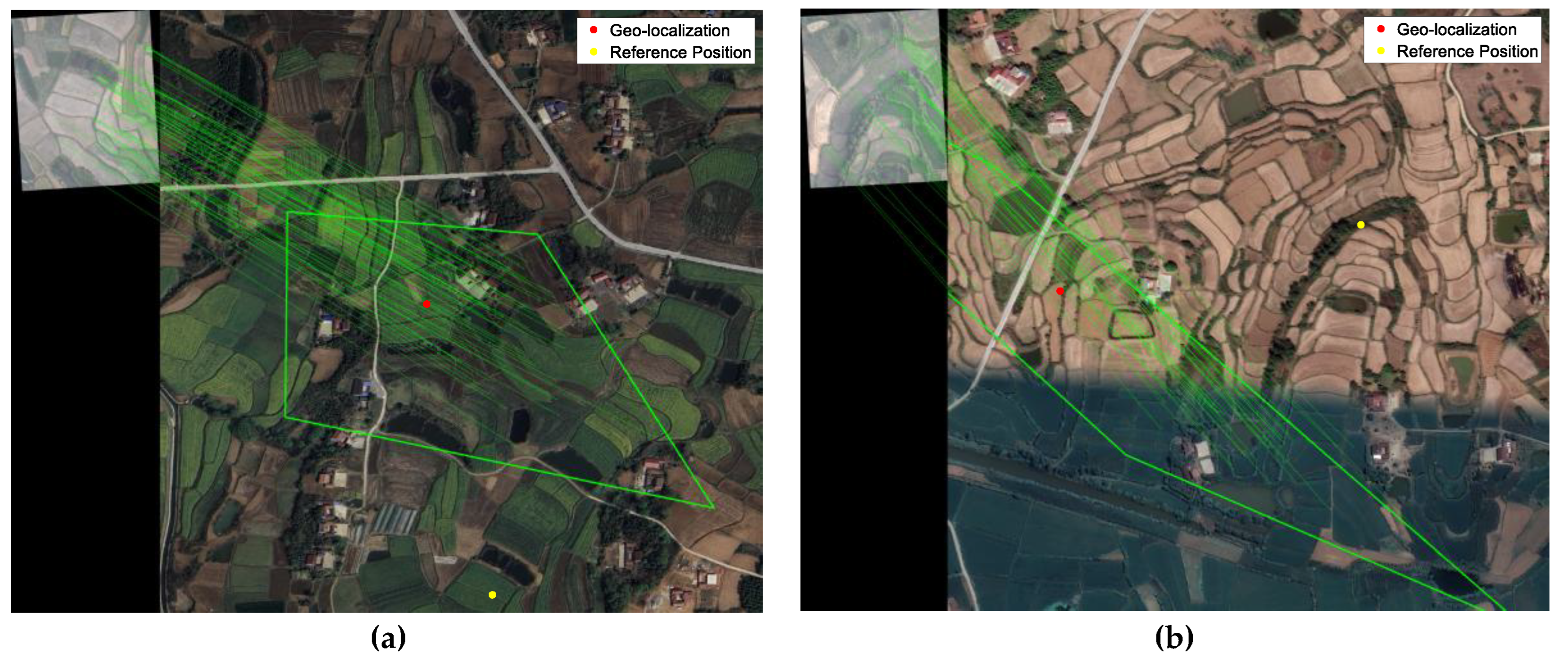
Table 1.
Reference map set index.
| Sub-map | Center of sub-map (longitude, latitude) |
Descriptors |
|---|---|---|
| … | … | … |
Table 3.
Parameters of Cameras.
| Visible Light Camera (Flir BFS-U3-51S5C-C) |
Thermal Camera (Guide Sensmart Plug617) |
|
|---|---|---|
| Resolution | ||
| Frequency | 1Hz | 1Hz |
Table 5.
Precision evaluation and comparison results.
| RMSE(m) | Max Linear Bias(m) | End Point Error(m) | |
|---|---|---|---|
| PINS | 450.933 | 890.55 | 627.49 |
|
Without Gaussian Elliptic Constraint |
112.65 | 423.65 | 75.10 |
| Proposed Method | 42.38 | 261.23 | 65.21 |
Disclaimer/Publisher’s Note: The statements, opinions and data contained in all publications are solely those of the individual author(s) and contributor(s) and not of MDPI and/or the editor(s). MDPI and/or the editor(s) disclaim responsibility for any injury to people or property resulting from any ideas, methods, instructions or products referred to in the content. |
© 2025 by the authors. Licensee MDPI, Basel, Switzerland. This article is an open access article distributed under the terms and conditions of the Creative Commons Attribution (CC BY) license (http://creativecommons.org/licenses/by/4.0/).
Copyright: This open access article is published under a Creative Commons CC BY 4.0 license, which permit the free download, distribution, and reuse, provided that the author and preprint are cited in any reuse.


