
Submitted:
06 February 2025
Posted:
07 February 2025
You are already at the latest version
Abstract
Increasingly larger turbines have led to a transition from surface-based “bottom-up” wind flow modelling and meteorological understanding, to more complex modelling of wind resources, energy yields, and site assessment. More expensive turbines, larger windfarms, and maturing commercialization have meant that uncertainty quantification (UQ) of such modelling has become crucial for the wind industry. Here we outline the meteorological roots of wind modelling and why it was possible, advancing to the more complex models needed for large wind turbines today, and the tradeoffs and implications of using such models. Statistical implications of how data is averaged and/or split in various resource assessment methodologies are also examined, and requirements for validation of classic and complex models are considered. Uncertainty quantification is outlined, and its current practice on the `wind’ side of the industry is discussed, including the emerging standard for such. Demonstrative examples are given for uncertainty propagation and multi-project performance versus uncertainty, with a final reminder about the distinction between UQ and risk.
Keywords:
wind energy
; boundary-layer meteorology
; uncertainty quantification
; wind resource assessment
; energy yield assessment
; micrometeorology
1. Introduction
In the age of multi-megawatt turbines, which began what I’ll roughly label as the `second generation’ of industrial wind energy, a number of significant differences have arisen compared to the first few decades (`first generation’) of the wind energy industry. Some of these changes have essentially come to crucially (re-)define industrial wind energy, from research to operation. This is true not only of wind energy as a whole, but also particularly within the areas related to quantitatively describing the wind, from meteorology to uncertainty quantification.
A single article about meteorology in wind energy would be too long (books such as [1,2,3] already exist), as would an article on uncertainty quantification in wind energy, about which a book could be written. The present article is thus centered on the emergence of UQ in wind energy, on the side of the primary ingredient in such energy production—the wind itself, as informed by applied meteorology and meteorological advances. This involves bridging from theory to practice, including the crucial statistical aspect of application and interpretation.
1.1. An Exceptional Multi-Disciplinary Problem
For wind energy production, our main `ingredient’—the wind—can be quite uncertain to quantitatively characterize in the long term, let alone predict in the short term. This is different than other industries, where individual ingredients in production are well-known or even quality-controlled.
The environment in which wind turbines operate, known as the atmospheric boundary layer (`ABL’), is one whose quantitative description involves a daunting number of physical variables—most of which range over multiple orders of magnitude, arising over and/or characterized by different lengthscales and timescales that also span numerous orders of magnitude [4,5,6]. With numerous flow regimes and behaviors that can depend on the time of day, season, geographic location, and distance from the surface, wind in the ABL—and UQ of wind resources within it—can be quite challenging.
As detailed in Section 2, the large number of physical variables describing flow in the ABL can be reduced from (at least) 10 down to seven by combining them into dimensionless groups, and perhaps further to four or fewer near the surface; the latter situation was exploited in the first generation of industrial wind energy (with its implicit assumptions persising in some IEC wind standards). However, non-stationarity of the flow and inhomogeneity of the flow environment complicate the picture, effectively adding several more variables to deal with, also outlined in the next section. Further, for large windfarms, particularly relevant offshore, the windfarm-atmosphere interaction introduces several more variables. Increases in turbine size have also meant that upper-ABL variables can no longer be neglected.
Thus, the statistics that wind engineers `think’ they get from measurements can be different than what has actually been obtained: such wind statistics are conditional on quantities which have either not been measured in a typical industrial pre-construction campaign, or accounted for in the statistical calculations. This has implications for measurement-driven modelling in wind energy, where models with a limited number of inputs are used to predict wind statistics and associated UQ at different sites; the uncertainty can depend on quantities that have not been measured. Doing UQ, validation and model parameter tuning is challenging here, because one essentially needs to account for the influence of numerous variables, including those which may vary from site to site. In order to cover a representative space, many simulations are needed, demanding an untenable amount of computational resources unless sufficiently simple (fast) models are used; there is a tradeoff between model complexity and ability to validate.
There is also the issue of workers, disciplines, and companies within wind energy having different engineering or scientific backgrounds and aims, which bring with them different nomenclature, terminology, assumptions, tools, and industrial practices. Many wind engineers have backgrounds more related to mechanical engineering or disciplines associated with wind turbines, with only a small minority having expertise in boundary-layer meteorology or applied statistics. To model complex systems lacking complete unified models, such as ABL flow (or wind turbine), it is worth noting that uncertainty quantification may demand more expertise in the area of application, compared to the modelling itself; one way of stating this is that simply running Monte Carlo simulations of a complicated model might not provide sufficient or applicable uncertainty estimates. Additionally, the quantities of interest, and assumptions about them, may differ depending on the application; e.g., some quantities demanded by both wind resource assessment and site assessment might differ depending on their use, and wind resource analysts may have substantially different understanding than loads engineers. The above aspects further lead to a level of community uncertainty, due to differing understandings and treatment of wind modelling. The latter can be accomodated by clearer reporting of industrial wind calculations, and is ultimately addressed by an industrial standard for wind modelling and its uncertainty; creation and finalization of such a standard (IEC 61400-15-2) has taken roughly one decade. The increase in the size of turbines and projects, with subsequently higher total costs and capitalization, as well as maturation of the commercial side of the wind industry, has also meant that the need for and value of UQ has dramatically increased in importance within the meteorologically associated areas of resource, energy yield, and site assessment.
The present work delves into describing the problem of industrial wind quantification by first describing the ABL parameter space via meteorological variables and proceeding into applied meteorology in Section 2. This is followed by statistical characterization and how it is practically applied in Section 3. Uncertainty quantification is the basis of Section 4, followed by industrial application in Section 5 and lastly some summarizing discussion.
2. Some Wind Energy Meteorology
2.1. Describing the Parameter Space for Wind
Flow in the ABL, can be considered most simply through the variables that describe it. These include the wind speed U for a given height z, the surface roughness length , the surface-layer kinematic stress (where is the near-surface air density), the surface-air heat flux , the Coriolis parameter (inverse timescale characterizing the Earth’s rotation effect on lateral motion as a function of latitude), the air’s viscosity , the ABL depth , the strength of the ABL-topping temperature inversion, and the strength of the large-scale horizontal pressure gradient driving the flow. Here by `large-scale’ we mean tens of kilometers or more, with the driving pressure gradient expressible in meters per second as the geostrophic wind defined by . The term `kinematic’ indicates a quantity normalized by the air density. Thus we use a kinematic viscosity , with units of m2s−1, and in micrometeorology the kinematic surface stress is expressed via the definition of friction velocity through ; here u and w are fluctuations about the mean for streamwise and vertical velocity components, angle brackets denote an average (typically 10 minutes), and subscript `0’ indicates near-surface, so the stress can be efffectively replaced by with units of m s−1. The ABL-capping inversion strength is commonly expressed via the Brunt-Väisälä frequency defined by the vertical gradient of virtual potential temperature1 (meteorological `lapse rate’) above the ABL () through where m s−1 is the acceleration due to gravity [4,8]. The surface heat flux can be simply described by the covariance of fluctuations in and vertical velocity (w), with units of degrees Kelvin times meters per second, as .
Using Buckingham-Pi analysis [9,10,11,12], one can identify the minimal number of variables needed to describe the system that we are considering, i.e., ABL flow. The Buckingham-Pi theorem states that a number of dimensionless variables are needed to describe a system, where is the number of dimensional variables and is the number of units involved in these variables. The list of variables from the previous paragraph gives ; the units describing these quantities are meters, seconds, and degrees Kelvin (since kinematic quantities lack kg), giving so that . Accordingly, from the meteorological and geophysical fluid dynamics literature we find seven non-dimensional `numbers’ or `groups’ describing atmospheric boundary layer flow:
- ABL Rossby number [20];
Here is the von Kármán constant, and is the Obukhov length. These dimensionless quantities can be seen to basically represent ratios between two (occasionally three) timescales, lengthscales, forces, or energies; they also arise when non-dimensionalizing different truncated forms of the Navier-Stokes (force balance) or kinetic energy balance equations [27]. Thus they typically tend to represent the dominance of one phenomenon or flow regime for very large values, and another for very small values, or conversely indicate that one term in a balance equation can be neglected (e.g., the viscous term in the Navier-Stokes equation becomes negligible for the large Re encountered in the atmosphere). So-called similarity theories can also be constructed which analytically describe flow behavior in certain limits [10], in terms of these variables (e.g., Monin-Obukhov similarity to treat buoyancy effects on the wind profile as a function of ). One can also find a few other parameters in the literature constructed with the same variables (e.g. , , ,27] or [5]); these are simply combinations of the parameters in the bullet-point list above.
Nonuniformity of the surfaces underneath an area of interest, such as hills or coastlines, will introduce additional length scales of horizontal inhomogeneity [4,28,29]. Further, geostrophic shear () arises due to large-scale horizontal temperature gradients, also known as baroclinity or baroclinic shear [30,31]. Consequently we have yet more variables to consider, in addition to the flow variables mentioned above. Temporal nonstationarity might further add a timescale to the list of variables to consider; however, this is typically not relevant other than perhaps wake-related load-associated areas such as meandering [32,33] or U-dependent decay [34]. Furthermore, windfarm scales including the rotor diameter, characteristic horizontal turbine spacing, and hub-height [35,36,37] can increase the variable space yet more; this can also include addition of wake blockage scales which combine with the earlier list of ABL variables e.g., stability, [38,39] to form more dimensionless groups.
2.2. First Applications of Meteorology in Wind Energy
The early days of wind energy—indeed the first generation of folks working on it—were both challenged by and benefitting from a particular aspect of the wind turbines in that era: they were generally confined to the atmospheric surface layer (`ASL’). The ASL is defined as the bottom ∼10% of the atmospheric boundary layer [4], which can vary hourly, with daily and seasonal patterns; can vary from less than 200 m to more than ten times that, most commonly having depths of ∼500–1000 m [40]. Thus in the first decades of wind energy, where hub heights were typically below ∼50 m with rotor tops often lower than m [41], then they were confined to the ASL, or at least most of the rotor was usually within the ASL. Here the surface dominates the flow, and the physics—i.e., the micrometeorology—are relatively well known; this formed the basis of wind resource assessment in the wind industry.
Generally in the ABL the Reynolds number is very large ( to ) so flow predictions do not depend on [4] and it may be neglected from the list given in the previous sub-section. In the ASL the effects of the ABL depth may be ignored, dropping the final three dimensionless variables from the dimensionless list in Section 2.1; we are then left with {, Ro0, }, along with needing to model the effects due to local inhomogeneities.
The first wind resource modelling with a micrometeorological basis basically addressed three elements: vertical extrapolation (VE) from measurement height to turbine hub height, horizontal extrapolation (HE) from a measurement mast to another location, and treatment of effects arising from surface inhomogeneities. To deal with surface inhomogeneities, i.e., terrain, originally the effects due to variations of surface elevation (hills) and surface roughness changes () were treated separately. That was accomplished through quasi-linearized modelling, using the assumption that terrain (orographic) effects on the flow can be superposed on effects due to surface roughness changes; perturbations of the wind speed at a given point relative to the wind speed over a flat uniform version of the surface are modelled as
where the are dimensionless wind speed perturbations due to the terrain inhomogeneities upwind in a given direction. The orographic perturbations, often labelled in WRA as “speed-ups,” were modelled using quasi-linearized Jackson-Hunt theory [42] applied within a cylindrical Fourier framework the `IBZ’ model [15,43]; implementations other than the WAsP/EWA [43] IBZ-model also exist, but have the same character (e.g., the so-called MS-Micro model). This modelling lacks turbulence and only applies to orography with limited steepness where slope-induced flow separation is negligible, and so consistent with (1) it is most accurate and usable when predicting . The effects of a surface roughness change—transition from an upwind windspeed profile above the so-called internal boundary layer to the local surface-induced profile—are basically handled by interpolation in assuming neutral conditions (without buoyancy effects); multiple roughness changes are handled by a multiplicative superposition model with spatial damping [15,44]. In terms of the augmented dimensionless parameter list from Section 2.1 which would include the addition of more parameters to deal with inhomogeneities, several modelling choices were made which avoid such large parameter space. Treating hills and roughness changes separately, neglecting the effect of stability and ABL depth in such treatment, and noting that the inhomogeneity effects are local so that Coriolis influence is negligible, together mean that we are still left with only ; the first two are known to affect the flow at larger scales, and arise in HE modelling, and is part of the VE modelling.
For horizontal extrapolation (HE), the geostrophic drag law (GDL)
was the first basis for HE in wind energy—if one dismisses the generally untenable practice of horizontally interpolating between two measurements [15]; consequently two of the dimensionless parameters () are reduced to one. Originally derived to relate the geostrophic drag coefficient to (that is to ) [16], its use in the EWA-method arose with the observation that the wind-driving pressure gradient (expressed via G) varies over scales of tens of kilometers—at least over un-mountainous terrain far from the equator, such as in northern and western Europe where the EWA was first made and validated. Thus for a potential turbine site not too distant from a measurement location, one can assume the (mean) G to be the same at the two sites; by using a wind profile model then one can obtain from winds measured at a mast location, calculte G using (2), then at the turbine location(s) calculate `new’ and .
For vertical extrapolation (VE), so-called similarity profiles have long been in use, such as the logarithmic wind profile which ignores buoyancy, and Monin-Obukhov similarity which correct sthe log-profile for non-neutral conditions based on . The EWA/WAsP incorporates GDL-based perturbations into Monin-Obukhov theory, leading to quite complicated expressions for stability-affected adjustment of the Weibull-A parameter at a given height relative to the surface roughness [45]. It is applied as a factor after `removing’ local terrain effects from observed winds via (1) just before GDL (2) use to get G, and just after subsequent GDL use to get at the prediction site before applying terrain effects there. The factor perturbing the logarithmic profile at observation or prediction site can be expressed as , meaning that the perturbation is simply also an additive correction to of the form
where is the effective Monin-Obukhov stability correction function accounting for the long-term mean effect (`offset’) and fluctuations (`rms’), is a scale height (ca. 65–80 m), with the offset heat flux and fluctuation amplitude in ∘K m s−1. The EWA method also perturbs the Weibull-k parameter per height for stability with analogous expressions [15,46], to predict Weibull distributions.
Alternately, in many industrial applications VE has been done using the power-law profile, which does not have a meteorological basis (though a meteorological connections were later derived [47,48]). By calculating the power-law exponent from winds measured at two heights ( then measured winds can be scaled by the factor to predict wind speed at height . To compare with the EWA perturbation form (3), binomial expansion gives an -based factor of .
The EWA and similar WRA methodologies could essentially be considered as perturbation-type models; for relatively small corrections to the observed wind and/or wind at prediction site, its symmetric modelling (where the GDL is applied alternately in opposite directions, as is the GDL-perturbed stability correction if it is used) means that the effect of biases in GDL parameters is reduced, since they are taken to be the same at both sites, other than . This can be seen by expressing the EWA method’s wind prediction based on observations:
where denotes the use of (2) and denotes the use of the inverse of (2), i.e., numerical solution of from G obtained by first use of the GDL; here is the VE model factor, whether calculated using the EWA form (3) or power-law (in the latter case ). Because the can be expressed as an additive perturbation for -based VE (given the values of and used in practice), and similarly for the EWA form (the ratio of disappears with the symmetric GDL double-use), then also satisfies superposition, like the terrain modelling. It can be written as , so that when multiplying by the local surface inhomogeneity corrections it becomes simply added to . If some flow perturbations become large enough, then the superposition assumption fails and results become more uncertain.
2.3. Meteorology Beyond the Surface-Layer
Farther from the surface, above the ASL where most multi-megawatt turbine rotors are located, two things generally happen to the flow: (1) the effects of surface inhomogeneities are reduced, with surface variations farther upwind increasingly affecting the flow (albeit more weakly) and with larger length scales characterizing the wind field; (2) more influence from the capping ABL-inversion is felt. Simply put, less `bottom-up’ effects, and more top-down effects are impacting the wind one looks above the ASL. So the amount of modelling needed to capture local hill and roughness effects tends to decrease above the ASL, though roughness changes such as coastlines that are farther away (∼50–100 times the z considered) can begin to affect the flow; but because the IBL grows with distance downwind of some , the blending (interpolation) between upwind and downwind profiles becomes spread over a larger vertical span. Generally the surface inhomogeneity aspect of wind resource prediction becomes easier above the ASL (smaller corrections), while the VE modelling gets more challenging.
Buoyancy effects associated with the surface are constant or decrease with height through the surface layer (the shear in stable conditions according to M-O theory, while decreases as in unstable/convective conditions [49]), with overall higher shear than neutral conditions due to the cumulative effect of stable stratification surpassing the mixing effect of unstable conditions [50]. However, for heights above the climatological mean ASL depth (typically 50 m or more), the picture gets more complicated. Long-term mean shear is increased due to the `top-down’ entrainment of very stable air from the capping inversion, with relatively rare shallow ABLs (low ) causing an outsized impact; on the other hand, tends to be larger in unstable conditions, which have a nearly zero-shear mixed layer around half the depth. [45] extended the form of [51] to capture the combined long-term mean effect of these, including distributions of stability and also adapting it to be consistent with the geostrophic drag law; the latter form was implemented in WAsP, has not gained operational release. [52] and [53] derived similarity theories to account for the strength of the inversion for a given ABL depth, extending wind profiles in a way that includes and the previously mentioned dimensionless parameters ; but such profile forms are not yet used in industrial WRA.
However, the full EWA method/WAsP actually includes a simple treatment of ABL depth in its vertical extrapolation; it damps the stability effect with height (as [15,54]), and also incorporates the mean effect of on perturbing for a given G [15,46]. The shear-perturbing effect of baroclinity (large-scale horizontal temperature gradients) and shear-increasing effect of the Coriolis force () derived by [55] were more recently added to WAsP [31,54,56], though for typical VE use (less than 50 m distance between prediction and measurement height) these perturb the speed significantly less than the surface stability.
Wake modelling has also come to include micrometeorology as turbines and windfarms grow larger, because wake recovery—and the energy available for large wind farms from above—depends on entrainment affected by the capping inversion; wakes are also affected by stability due to surface heat fluxes. The recent wake model of [57] integrates all the aforementioned effects (ABL depth, inversion strength, surface heat fluxes), though it is not yet in common use. Industrial EYA tends to involve simpler engineering wake models, which lack meteorological basis. Blockage is also known to be affected by stability due to the capping inversion [58] and also surface fluxes [38], but models including these effects have not yet been adapted into most industry workflows. An exception is Fuga [59] (currently via open-source pywake [60], which incorporates surface-layer M-O similarity for both wake deficit and blockage, though it does not treat top-down effects due to and .
2.4. More Advanced Modelling...
2.4.1. RANS Modelling
CFD, particularly RANS solvers, tend to lack much of the meteorology affecting the wind. This is due in part to the difficulty of where RANS solutions are used, namely over complex terrain. In such areas with intermittent recirculation, such as behind hills, a mean solution may be nonsensical due to multiple flow regimes and a local velocity (or speed) distribution which is not unimodal; adding extra physics into the RANS equations and solver can make convergence to a mean solution even more difficult, and more dependent on the expertise of the person using the solver. Unlike simplified flow models such as the EWA/IBZ mentioned earlier, RANS solvers do not separately model hill-induced speedups and perturbations due to roughness changes; rather, these arise in solution of the RANS equations due to the terrain elevation and variations being prescribed through lower boundary conditions, along with stability effects arising from prescribed surface temperatures or . Thus, these different phenomena can interact together, with larger perturbations possible and no superposition or its requirements.
In non-neutral conditions the ability to use a RANS solver to determine the speedups independent of wind speed disappears, as the appearance of buoyancy causes a wind-speed (actually Froude-number) dependence in the nondimensionalized RANS equations. The same thing occurs if one includes the Coriolis force: again a wind-speed dependence appears, via Rossby number in the normalized RANS equations. To show this one can normalize the vector RANS equation by rewriting it with normalized variables , assuming characteristic length and velocity scales and to substitute with and , and also with Reynolds-stress tensor [4,61]. Noting that in -space and then dividing the whole equation by , we obtain the RANS equation in terms of the nondimensional variables:
here the Rossby number is , and the Froude number is . We see that over sufficiently long horizontal distances per wind speed (where ), e.g., in mid-latitudes with s−1 then for mean winds of 10 m s−1 the Coriolis term will become significant over distances of km or more; this is relevant in large windfarms and where neighboring farms exist. For buoyancy (5) seems to indicate that only the vertical velocity is affected, but it turns out that a contribution to horizontal velocity arises through the (turbulent) Reynolds stress divergence [62], of order [47].
Related to the above is the difficulty of RANS solvers in capturing unstable (convective) conditions over hilly terrain, where large circulating eddies can arise both due to buoyancy and the terrain shapes, and tend to defy mean solution. Further, solving flows over complex terrain in stably-stratified conditions has not yet been shown to be universally acheivable using conventional (1- or 2-equation) turbulence closures, though there is some commercial software which does so via implicit damping or limitation of the terrain and buoyancy effects (thus approximately treating such). RANS with higher-order algebraic models have recently made this more possible (e.g., explicit algebraic Reynolds-stress models [63,64]), but are not yet used industrially. At any rate, use of RANS solvers with stability and/or Coriolis requires multiple simulations at different speeds per wind direction, with stability also requiring simulations for different stabilities in order to attempt to represent long-term effects [65]. Subsequently, validating them requires covering a larger joint variable space due to the addition of two variables (or more, if a capping inversion is imposed).
2.4.2. Mesoscale Modelling
On the other hand, mesoscale numerical weather prediction (NWP) models such as WRF (the Weather Research and Forecasting model) are built on meteorology, though they tend to have effective resolutions [66] of several kilometers; thus they capture the physics at these (meso) scales, but not turbulence nor local terrain effects. The latter can lead to prediction bias onshore [67], with offshore bias also occuring due to several factors e.g., [68]. Hills, roughness changes, and heat fluxes are bottom boundary conditions, just as with CFD. However, NWP resolutions mean that hills are smoothed out, so cannot be very steep; and NWP does not give -induced IBLs matching microscale models or theory, but rather an analogous adjustment of the flow depending on the NWP advection scheme [69,70]. As opposed to the mean values (per specified boundary conditions) given by RANS solvers, NWP gives timeseries, including time-varying values of surface heat fluxes, temperature and heat flux profiles (thus implied associated inversion heights and strengths). Several years of NWP data tends to cover the 7-dimensional space listed in Section 2.1, but the (joint) PDFs of the variables may be limited by the duration of timeseries, as well as model resolution and turbulent flux parameterization (planetary boundary layer or `PBL’ scheme) e.g., [71].
NWP models are nonetheless commonly used for long-term correction, as their biases can be removed by incorporating the measurements, while long NWP model timeseries (many years) allow compensation for measurements occuring in windy or weak-wind years relative to means over expected turbine lifetimes (decades). NWP models are also gaining increasing use for HE and flow adjustment in geographical areas where mesoscale effects cause significant differences between measurement and assessment locations; in industrial WRA mesoscale results are sometimes also `blended’ with classic HE calculations to constrain issues due to resolution or biases. Mesoscale model calculations for WRA require significant expertise and resources, as noted in the review of Haupt et al. [72] on numerical weather prediction for renewable energy.
NWP has also been used to create so-called wind atlases at national, regional, and global scales, by using the GDL to `downscale’ is output [73,74]. These basically employ NWP output as a virtual mast over the mesoscale surface map, then apply the EWA methodology ala (2) and (4) to predict on a much finer grid using a microscale surface map along with the EWA microscale modelling; the wind atlases essentially give Weibull parameters and mean winds, though the New European Wind Atlas (NEWA) [75] and newer versions of the Global Wind Atlas (GWA) [76] offer more statistics.
3. Appropriate Statistical Characterization, from Theory to Practice
Much of applied meteorology in wind energy is inextricably related to statistical characterization and subsequent interpretation, dependent on the application or even use case. One can view this as stemming from the nonlinearity of the Navier-Stokes equations and horizontally inhomogeneous boundary conditions or nonstationarity, the character of wind variations depending on the length and/or time scales over which the wind field is calculated, and also nonlinearity in typical turbine power curves. We remind that averaging a nonlinear function of a variable does not give the same result as evaluating the same function using the average value of its input variable, , whether it is a temporal or spatial average; hourly, monthly, and yearly statistics of the wind differ from each other, as do microscale and mesoscale motions.
3.1. Rational Averaging Implicit in Classic WRA
For wind resource assessment the dominant methodology since the 1990’s, following from the EWA method [15]), calculates long-term wind statistics (histograms or Weibull parameters) that are representative for a turbine lifetime at a given site; the wind statistics are essentially representative for an “average year”. One convenient advantage of doing this (perhaps a neccessity in the creation of the EWA) is that the geostrophic drag can be essentially reduced as a variable: by taking the long-term average of (2) and knowing the GDL’s sensitivity to the parameters , one may use characteristic long-term values of —presuming that they do not still depend on other parameters after such averaging; the becomes a function of climatological-mean , as implemented in software such as WAsP [77] and wind atlases using the EWA methodology [78,80,81]. So it becomes possible to use the GDL for horizontal extrapolation from one site to another wherever the GDL is applicable, without considering other variables as long as the ABL top is not causing a large mean impact, to the extent that are representative; as noted in [20], `default’ values of used in the aforementioned implementations were empirically chosen as a compromise to allow use over both land and sea. The previous section also showed the EWA method/WAsP does incorporate the mean effect of the ABL depth on the GDL through perturbation of the surface heat flux to account for the change in due to surface-driven stability and ABL depth through , using mean values of [15,46].
The EWA method, designed to be driven by measurements with its two-way “up-down” use of both the GDL and long-term stability perturbations, essentially reduces the influence of uncertainties in its GDL and VE-model parameters because any biases in them cancel to first-order in (4) due to appearing in both numerator and denominator, leaving only higher-order (smaller) contributions. However, `one-way’ use of the GDL is more prone to systematic uncertainty (bias) in its constants, which is one reason why one cannot use pressure gradients from mesoscale modelling or measurements and obtain reliable results.
3.2. Refined Modelling and Consequent Sampling Issues
In general the more that one divides data into separate categories, the higher the sampling uncertainty becomes; alternately, the higher the demands on sampling are for a given uncertainty tolerance (e.g., see Ch. 2 of [4] for the generic case of means of a stochastic signal). In wind resource assessment, the practice of using a 24×12 “matrix” — where measurement data is separated into hour of the day per month of the year — is intended to better accommodate the different flow regimes occurring during the diurnal and seasonal cycles, towards better predicting the wind resource and energy production based on measurements. Dividing measurements into 288 (24x12) time-categories for modelling gives ∼180 samples per bin per year of data, which appears reasonable; but a histogram or Weibull fit requires or more samples to have a reasonable shape. Subsequently separating per wind direction then further reduces statistical representativity. Further, doing such `chopping’ assumes that the WRA modelling can properly treat the flow regimes occurring at different times, and that these models are somehow informed by the additional information relevant to characterizing these regimes.
For example, nighttime and winter periods over land will tend to be affected more by stably-stratified conditions from the surface as well as shallower ABL depths. For vertical extrapolation (VE), from these periods one needs to capture the and possibly effect, but using the power-law with shear measurements below hub height doesn’t capture the second; using M-O profiles for VE such as the EWA form (3) would require the ABL depth to be adjusted, in addition to the stability corresponding to the time/month regime. For horizontal extrapolation (HE) use of a RANS solver also requires representative and , while the geostrophic drag law (GDL) then requires its and -parameters to be modified for the specific conditions. Not accounting for these aspects adds uncertainty to the modelling, including possible bias, and potentially worsens the result at some sites compared to use of yearly means without such data division. A similar example can be considered offshore: sampling of winds in the North Sea far offshore. There, in the spring winds with southerly components will tend to induce stable conditions due to the water remaining cold from winter, and so again certain months in a 24x12 matrix would need to have GDL and stability parameters adjusted—but depending on wind direction.
To get around the problem of limited sampling, particularly offshore, more industrial use has been made of long-term re-analysis datasets such as ERA5, and multi-decade mesoscale datasets. These can give full wind PDFs even after dividing per hour, month, and direction, though they must be adjusted to correct their bias using measurements. However, the seasonal and daily variations in these datasets tend to be smaller than measured, though borrowing from the weather community one may use a combination of datasets along with techniques such as logistic regression or linear variance calibration [72].
3.3. Averaging Issues Arising with Timeseries Use or Comparisons
If one tries to use common WRA methodologies such as the EWA for predicting timeseries, a problem connected with that described in Section 3.2 can arise. That is, different values of the various modelling parameters, which have been defined and/or calibrated for long-term mean usage, must be modified to be appropriate for the conditions in each timestep. Further, the assumption of independent effects (allowing superposition) may become untenable with timeseries; in reality for times having non-neutral conditions the effects due to hills and roughness changes may be different than the flow-perturbation modelling (which assumes the long-term mean gives neutral conditions). In some cases this does not incur much uncertainty, such as GDL use in some simple offshore settings, but for inhomogeneous projects particularly over land the accuracy may be reduced and uncertainty increased.
Another issue arises with mesoscale timeseries, when comparing with or attempting to directly supplement measured timeseries per timestamp. Known as a `phase lag’ problem, it is the phenomenon whereby mesoscale predictions can have a horizontal and temporal offset (`lag’) compared to reality, thus making comparisons difficult. Different methods exist such as filtering out periods where the timeseries have a correlation coefficient falling below some threshold, but these are not yet standard practice.
Another averaging issue which involves comparison is the width of directional sectors used when comparing observations to wake models [79]. Basically the sector width must be sufficiently larger than the directional uncertainty (standard deviation of direction) in order to compare statistics. (A more general version of this might be considered for comparisons conditional on other quantities beyond direction.)
4. Uncertainty Quantification
Models for different effects on the wind all propagate—and potentially amplify—uncertainties in their inputs, while also adding their own additional uncertainty independent of the measurements. For measurement-driven modelling, which is standard in bankable energy-yield assessment, this begins with wind measurement uncertainty.
The Guide to the expression of uncertainty in measurements (`GUM’) [80] can be seen as a basis reference for much UQ work in wind energy, including propagation of measurement uncertainty; its initial (concurrent 2008) supplement [81] gives guidance for propagation of distributions via Monte Carlo methods, and and its second (2011) supplement [82] extended to multiple quantities. The more recent (2023) GUM `introduction’ [83] outlines how GUM and all of its supplements can be used; notable is the 2020 supplement on models [84] which includes addressing poorly understood effects, shared (correlated) effects, and basic model uncertainty.
GUM essentially provides a description of first-order uncertainty estimation via propagation of measured uncertainty; this uses Taylor series to give a linear (approximate) response of a model around the expected value of its input x. This can be expressed as where is the model sensitivity in the neighborhood of ; note this can change if is different. This leads to
where the are the uncertainties, i.e. standard deviations of x and y (see uncertainty textbooks such as [85] for more details). When uncertainties are small compared to the actual values of measurand(s) () and the sensitivity does not change too quickly with x compared to (like ) then (6) is a useful approximation, not requiring higher-order terms. Following GUM, the actual value of a measured quantity x follows either a normal distribution (`Type A’) or a unit distribution (`Type B’), with different uncertainty types combinable by scaling type B variances () with a coverage factor of 1/3 and summing the squares to find total squared uncertainty [80]. Such summation presumes independent uncertainty components having the same units, or that each uncertainty is nondimensionalized by its respective mean. (6) can also be generalized to include a vector representing multiple inputs and for multiple outputs, incorporating the covariances between all of these [85].
For highly nonlinear processes and models, the low-order GUM technique begins to fail due to sharp changes in model sensitivity. A way around this is to use Monte Carlo `simulations,’ whereby the model calculation is repeated many times, but with its input(s) taken from a random (joint) distribution that reflects the uncertainty in the input(s). For example, Figure shows the power output from a Monte Carlo where randomly sampled speeds are put into a simple power curve, where the expected speed is and its uncertainty is (6%) and the error is normally distributed; the GUM result following (6) is also shown.
One can see from Figure 1 that GUM fails around rated speed, due to the sharpness of the power curve there. In cases/applications such as this example where a bi-modal distribution results, one must consider not only using a Monte-Carlo or other method, but possibly also consider output uncertainty metrics such as or others. The demonstration above used points, but still one can see considerable noise in the PDF; in this case (not shown) the Monte-Carlo curve becomes smooth for points. This reminds of the sampling demand when using Monte Carlo simulations, meaning that it becomes computationally difficult to do them for more than a few dimensions; other more advanced methods are possible, as outlined and used e.g., in [6].
4.1. Uncertainty in the Complex ABL System
The uncertainty and validation framework of Huard & Mailhot [86], which is visualized in Figure 2 as adapted by Murcia [87], further indicates that UQ and validation have a conditional or Bayesian aspect.
In Figure 2 one sees that for validation the outputs of a complex model having multiple inputs (vector ) and model parameters (vector ), require validation conditional on model error as well as on , , , and . It also indicates that optimal tuning of parameters is also conditional on these latter three. Forbes [88] showed how the classic GUM method is an approximate solution to the Bayesian approach. [89,90,91] showed how and why GUM was updated, to accommodate and be consistent with Bayesian Monte Carlo methods.
But given the discussion in Section 1.1 and list of inputs such as that shown in Section 2.1 for advanced ABL models, we cannot easily validate or tune models unless we have a large number of sites and measurements spanning the multi-dimensional space —i.e., actually knowing the relevant variables which our results are conditioned upon, including those describing inhomogeneity, as well as sensitivity of the model to all these. An exception to this is the EWA method, whereby within its operational design envelope, the number of parameters becomes manageable, particularly at non-complex sites; this is one reason the EWA method and software has been used for bankable WRA over several decades. Mesoscale (numerical weather prediction) models and RANS (CFD) solvers can treat the effects of more phenomena and more variables, but paradoxically then require a larger validation space ; they are currently too computationally demanding to run millions of times in order to cover the dimensional space involved. Other exceptions to this are engineering models such as those used for calculating wakes within a wind farm.
The Validation and Verification (V&V) framework of [92] offers one way to address the computational complexity issue, including the so-called `PIRT’ (Phenomenon Identification and Ranking Table) which uses industry-wide expert knowledge to identify (typical) model weaknesses and reasonable operational envelopes. This framework originally arose to deal with complicated CFD calculations for heat transfer in other industries [93], but the latter did not deal with such extensive input spaces and infinite degree-of-freedom modelling as we have in the ABL; thus it has informed some emerging practices in industrial wind calculation, but is not used for wind CFD yet.
In essence the first Comparative Resource and Energy Yield Assessment Procedures (CREYAP) campaigns [94,95] did something like the PIRT suggested by [92], identifying problem areas in the WRA-EYA process, and with the CREYAP-summary work of [96] evaluating the relative importance of different steps in the process.
Offshore, UQ could be considered a `simpler’ task than onshore, with narrower ranges of secondary variables involved (e.g., ABL depth and surface stability) and greatly reduced effects of inhomogeneity, particularly as floating lidar measurements have become standard practice and thus eliminate the need for vertical extrapolation. However, offshore projects tend to be larger, with more complex wake effects and potentially significant blockage; they also have taller turbines which interact more with finite-ABL effects. Further, offshore windfarms can be affected by other large windfarms at distances of several kilometers or more, requiring mesoscale modelling or modification of typical engineering wake models [97,98]. The offshore CREYAP exercises [99,100,101] gave indication of primary uncertainty components and some of their magnitudes in resource assessment offshore, though did not explicitly address some of the issues mentioned above. Beyond the CREYAP experiments, following the Sandia [92] V&V work, recently [102] gave a systematic framework for offshore V&V, which outlines future experiment concepts and essentially (implicitly) facilitates better UQ offshore.
5. Industrial Application
The way in which measurements and modelling of the wind field impact wind energy involves a web of processes and methodologies. To provide context, Figure 3 gives an example of a simple `digital model’ depiction (one-way coupling without automation [103]) of the complicated interconnected context within which meteorology fits into wind energy—and subsequently how uncertainty on the `wind side’ can propagate through model chains in different parts of the industry.
As seen at the top of Figure 3, wind measurements and meteorological model data can enter into both long-term pre-construction calculations, which are the focus of this article, as well as short-term operational modelling. Depending on how much integration and connection of models one wishes to pursue, observed and modelled wind data—and its uncertainty—can propagate well beyond wind resource & energy-yield assessment and siting, to regional (e.g. grid) planning in the long term; and windfarm operation/control, lifetime management, grid/transmission re-configuration, and energy trading in the shorter term. Regarding the interconnectedness shown in Figure 3 with many models coupled together, we note that there can also be uncertainty in the coupling itself; however, this is beyond the scope of the current article.
5.1. Wind Resources
This section will primarily focus on long-term wind resource assessment (WRA), which drives energy yield assessment (EYA), in the so-called pre-construction (planning) context; this contrasts with short-term forecasting and the operational context.
Given the number of different methodologies across the industry, the increased use of ensembles of model types and data, and the number of (often unmeasured) variables in the ABL as well as its complexity, the industry has progressed phenomenologically—as mentioned in the previous section regarding the CREYAP exercises—towards simple UQ based on engineers’ experience. Also guided by GUM, the IEC 61400-15 working group (on the order of 100 members) separated WRA and EYA uncertainty into components and sub-components, quantifying each of them through a consensus process based on expertise, aggregation of their industrial UQ practices and workflows, uncertainty modelling directly derived from certain WRA processes, and knowledge of (proprietary) production error statistics and associated pre-construction uncertainty estimates. An aim of this basic UQ is to not just establish a standard practice, but also facilitate reporting of uncertainties in order to reduce the variability in pre-construction uncertainty estimates from one engineer or company to the next. As discussed below in Section 5.5, an associated goal is to support reporting of UQ in WRA and EYA in order to separate uncertainty from (subjective) assignment of risk.
For wind-related (meteorological) uncertainties, the IEC working group established five categories, which are shown in Table 1. A sixth component (plant performance) is calculated in terms of energy production uncertainty, but has a wind-related subcomponent due to wakes and blockage.
The uncertainties in Table 1 are all calculated as normalized values, i.e., as a fraction of expected wind speed (expressible as a percentage), so that they may be combined to give a final total uncertainty. Each sub-component is also assumed to characterize normally-distributed variability. With the exception of power-law VE, whose uncertainty was derived analytically, the other uncertainty components and subcomponents are assigned based on conditions present in a pre-construction project, which a user of the emerging standard enters; the values per condition are based on project experience and expertise across the roughly 100 wind engineers, other IEC 61400 standards, and extant wind industry UQ workflows, and were re-calibrated based on cross-testing by the IEC working group. The various wind-related components are described below.
5.1.1. Wind Uncertainty Components
Measurement
Building from and consistent with the IEC 61400-50 series [104,105,106,107], IEC 61400-12 series [108,109,110,111,112], and MEASNET [113], measurement uncertainty subcomponents include contributions from station-level (documentation), monitoring level (data acquisition system and sensor combination), and sensor level (mounting, sensor classification/rating). The subcategories of wind speed and direction measurement both have these contributions, with the assumptions that abberent data and outliers have been removed, and that boom vibrations are damped/filtered away (neglected). It sums the squares of subcomponent variances, including sensor calibration, sensor classification, sensor mounting, flow distortion, and data acquisition. Formulae for these stem from the standards mentioned above.
Long-term correction
A number of different methods and datasets are used for LTC of measured data, with ensembles of datasets and correction methods sometimes employed. Thus for UQ of LTC, the adjustment is generalized, and to some extent is proportional to the long-term correction itself. Subcomponents include interannual variability adjusted for length of reference data set, reference data consistency, method consistency, gap-fillng, measured data representativeness, and wind distribution fit (if applicable); a uncertainty reduction due to ensemble usage is also considered.
Flow modelling and Horizontal Extrapolation
Because nonlinear models have been increasingly used in places with complex terrain (RANS solvers for forests or steep hills) and over areas where mesoscale effects are not captured by the EWA methodology (e.g., mesoscale models for parts of the central USA), industrial wind modellers in the IEC 61400-15 working group generalize HE and flow modelling together. That is, a flow model whose domain covers both the measurement and windfarm site(s) in effect also does horizontal extrapolation, in addition to treating the effects of orography, roughness changes, and sometimes stability (for mesoscale models and some RANS).
For horizontal extrapolation, the so-called `Clerc-model’ [114] was made for the EWA methodology, taking the IBZ flow model, roughness-change model, and the GDL together. It quantifies uncertainty basically based on the amount of flow correction (`speedup’) applied, along with the distance of horizontal extrapolation; it was been calibrated and used by several companies for more than a decade. However, from e.g.. [115] one sees that the HE uncertainty can depend significantly upon height beyond the amount of speedup, due to terrain complexity (basically from [29]). For this reason, and due to other complicating factors not included in the Clerc model, the 61400-15 HE subgroup created a model to quantify HE uncertainty including additional factors. These include accuracy of the terrain map coordinates, elevation and roughness data (including forest info), accuracy of input stability conditions required for a site, degree of site complexity (slopes, forestry, stability), limitations of model physics (flow separation/turbulence, stability, thermally-driven flow), suitability of computational resolution and domain size, and demonstrated accuracy of previous application of the model under similar conditions; for each factor a value is assigned based on whether it in considered to be low, moderate, or high uncertainty. The HE UQ model also adjusts for cross-predicion errors measured across multiple masts, and includes extrapolation distance as well as amount of correction (speedup and turning). Arising from evaluation of many pre- and post-construction sites, it essentially acts as a `pre-validated’ UQ model, and was calibrated and checked with additional sites from the working group. It allows both WAsP-like/EWA calculations as well as RANS solvers.
Vertical Extrapolation
The VE uncertainty was derived analytically for shear-exponent extrapolation, and calibrated with roughly 100 sites as reported in [116]. This applies to the application of shear-extrapolation per every 10-minute period, which has become a nearly standard way of using the power-law [117]. The VE UQ propagates measurement uncertainty, along with amplifying it depending on the shear exponent and prediction and measurement heights, with adjustment for terrain complexity and low-shear offshore conditions.
An UQ form for the EWA-extrapolation is not included, as the only existing form of [118] lacks dependence which may lead to systematic errors; a more complicated form including roughness has been derived, but needs re-validation due to improvements since its creation (updates that include e.g. use of re-analysis data to improve the stability [54]), complicating the WAsP VE.
Year-to-year project variability
The yearly project evaluation period availability uncertainty is calculated in order to be able to give estimates of or over different time horizons, say 10 or 20 years. This includes interannual variability and expected wind modification due to climate change. For a given project evaluation period in years () the IAV contributes a variance of to the total uncertainty squared.
Wakes and blockage
Under the plant performance uncertainty component there is one wind-based subcomponent, namely wakes and blockage/windfarm-air interaction effects. This is expressed as percentage of wind farm energy yield; it includes subcomponents of internal, external, and future wakes as well as internal, external, and future blockage effects. It is essentially proportional to the estimated losses, and also includes reduction for having more validation cases.
5.1.2. Combination of Uncertainty Componennts
The combination of wind uncertainty components is most generally calculated via
where the tilde indicates nonormalized quantities (components as percent/100), and are the correlation coefficients between pairs of uncertainty components and ; this is in line with GUM [80]. The IEC 61400-15 group consensus is to assume all for simple calculations; however it is known that some of them can be nonzero (e.g., between HE and VE). The use of multiple masts (measurement locations) is also addressed, by the summation for each uncertainty component
where is the normalized wind uncertainty component (as a fraction of wind speed) for mast number m, is the fraction of plant energy represented per mast m, and are the cross-mast correlation coefficients. Thus for , different masts add more information and thus act to reduce the uncertainty for components that are decorrelated across a mast pair. Such decorrelations may arise for LTC, measurements, and VE, possibly others.
5.1.3. From Wind to Energy
Energy production, particularly in wind farms, tends to be a complicated nonlinear function of measured wind speed statistics. However, we need to convert wind speed uncertainties into energy uncertainties, in order to combine with energy-based uncertainties as well as find the overall uncertainty in pre-construction yield (or e.g. ). In essence we need to find in order to do so. Near the calculated expected value of AEP (E) one may simply approximate this derivative by re-calculating the AEP for values of input speed above and below what has been used in the original calculation. This can be directly done by simply inflating and deflating the input wind data by scaling it with and finite-differencing. This can also be extended to Monte Carlo of the AEP calculation, using a Gaussian distribution of multipliers centered around 1 and having width . (The latter might be seen as a `cheap’ way to practically supersede the issue of dealing with many variable dimensions in the modelling, as a rough approximation, but only in the limit that the propagation of measurement uncertainty is the dominant contribution; we note this is just a crude estimate, and if model uncertainties unrelated to the wind measurement uncertainty are significant, this approximation does not work).
5.2. Forecasting
Yan et al. [119] reviewed uncertainties in short-term forecasting, i.e., prediction of power at horizons from less than an hour to a day or more into the future; these are used within the context of energy trading and adjusting production based on demand and cost. As [119] outlined, short-term operational forecasts are made more often by machine-learning methods than by meteorological models, though short-term meteorological ensembles can offer some degree of uncertainty estimation in the through their ensemble spread [120] rather than through detailed sensitivity and model uncertainty analysis.
5.3. Wind Atlases and Assessments Without Measurements
Intended for wind resource `prospecting’, datasets such as the Global Wind Atlas [76] and New European Wind Atlas [121] were not designed for bankable resource assessment, but rather for scoping out potential areas of development. But, it is probable that a (currently) small fraction of sites can be served solely by wind atlas or mesoscale data, alebeit with larger uncertainty than would be afforded by conventional measurement-driven WRA following best practices. Currently such atlases do not contain uncertainty, but this is part of ongoing work.
5.4. Siting, Design, and Standards
Second order moments, such as the variance of turbulent fluctuations, require longer averaging times (more samples) compared to simple first moments (mean values) to have the same sampling uncertainty [122]. Thus uncertainties on turbulence intensity tend to be higher than wind speed, also because turbulence is more variable and sensitive to local terrain and stability effects. [6] found the quantities most affecting loads to be mean wind speed, along with turbulence intensity and turbulence length scale, in that order. These are also key parameters for siting, along with site-specific extreme (expected 50-year maximum) wind speed . Generally RANS does not (yet) predict turbulence intensity as well as wind speed, and mesoscale or re-analysis data does not help, in contrast with mean wind speed and direction. Further, neither VE nor HE of turbulence has a standard practice due to the above reasons, and subsequently UQ of turbulence is difficult. The MEASNET guideline [123] addresses site parameters, as does the 61400-15-1 [124], giving a framework for reporting of these parameters towards uncertainty characterization.
5.5. Distinction from Risk
The ultimate aim with UQ is to estimate uncertainty distribution widths around predicted mean or median quantities such as wind speed or AEP, based on distributions of all the inputs to WRA and EYA modelling. We remind that use of input and component uncertainties can depend on how variables are used, as well as how they are determined. As der Kiureghian & Ditlevsen wrote in their seminal work on quantifying different types of uncertainty [125], “the nature of uncertainties and how one deals with them depends on the context and application.” For example, roughness length () has a log-normal uncertainty distribution and multiplicative uncertainty of nearly , seemingly quite large. But this variable always occurs as , which tends to be normally distributed and with corresponding uncertainty (standard deviation) from measurements of about 5% or less; however, assigned by wind engineers based on their experience can be ∼10–50% or more [126].
The UQ prescription by the IEC work group for the emerging 61400-15-2 standard, which includes a worksheet for calculations, mostly involve assignment of situation or condition-based subsubcomponent uncertainty values, which are combined assuming independence of components, as mentioned above in Section 5.1.2. However, along with the directly propagated uncertainties in the VE component, these were created to reflect underlying distributions without adding percieved risk as a bias or inflation of standard deviations. In previous years, uncertainty estimation did not necessarily reflect this practice, as conservative pre-construction uncertainty estimates were sometimes used, and with different consultants and companies having different assumptions and methods. An example of pre-construction uncertainty versus operational performance is shown in Figure 4 for more than 100 projects.
The data was from two large companies, with two UQ practices, from a decade ago (2005–2014). Across industry these vary, with likely yet more spread than shown in the figure. One can see some evidence of conservatism, for projects with uncertainties higher than about 7%, while the conditional standard deviation for those lower than 7% (using overlapping bins of width 1.5% every 0.8%) roughly matches the 1:1 line. For the projects with higher perceived uncertainty, the AEP error did not really follow pre-construction uncertainty estimates, nor did the mean bias. Overall the projects underperformed by about 1.6%, shown by the thick dashed line in Figure 4. It is worth noting that [128] showed that mean AEP overprediction has decreased over time, and that the numbers shown in the plot would likely be different if calculated today for the same projects and by the same companies. Other firms would likely give yet different results, but with a sufficient standard practice the expectation is that the dotted lines would overlap the green lines in Figure 4 while the thick dashed line (overprediction bias) would be at 0.
6. Summary
Here we have taken a summarizing tour from micrometeorology applied since the first generation of the wind energy industry, to uncertainty quantification in the next generation. The exceptional problem of wind resource assessment—prediction in a typically turbulent environment that is affected by many more variables than commonly measured in industrial practice—is outlined, starting with the nondimensional space that describes flow in the atmospheric boundary layer. An explanation of fundamental WRA methodology is given, including the basic equations explaining its model chain. We see how the classic measurement-driven EWA methodology greatly simplified the variable space that needs to be covered, sufficient for the first decades of wind turbines residing mostly inside the atmospheric surface layer. Consequences of needing to model the resources for taller turbines, and of using more complex models such as CFD and NWP to do so, are outlined. It is seen that modelling more physical phenomena requires knowledge of more atmospheric quantities, and makes validation more difficult, even if it increases accuracy. The benefits and implications of long-term averages and data splitting are examined, around the concept of sufficient sampling. We see that older climatological-mean formulations were designed to produce long-term statistics, while use of more complex modelling requires some expertise and potentially extra consideration in order to give representative statistics which reap the benefits of added model physics. This leads to uncertainty quantification, which is outlined in brief following the mutli-industry standard GUM [80]. The limitations of first-order UQ are examined, and the commonly used Monte Carlo method is introduced in the context of WRA and EYA. Current wind industry practices and findings in UQ of resource and energy prediction are noted along with the context of these and wind prediction within the industry overall, and the emerging IEC standard on such is outlined as well. Examples and reminders of the difference between risk and uncertainty are considered, motivating the need for and emergence of a standard.
Future needs and work involves standardized reporting of WRA and EYA methods used in wind projects, along with the UQ calculations associated with these. Further development of uncertainty (sub-)component models, based more directly on the WRA/EYA models used and able to propagate input uncertainties, still remains. Sharing of data across industry and academia is still a lingering need, which allows progress in this area that ultimately reduces project finance costs. Ongoing study of the value of uncertainty estimates to different parts of the combined wind energy-electrical-market system is also beneficial.
Funding
This work received no external funding.
Data Availability Statement
Not applicable.
Acknowledgments
The author wishes to thank Jake Badger for internal support of advancing UQ knowledge and application from DTU to industry; and Taylor Geer, Jason Fields, Gibson Kersting, Steve Clark, Martin Strack, and many other industrial colleagues for UQ discussions and work towards developing an IEC wind UQ standard.
Conflicts of Interest
The author declares no conflict(s) of interest.
Abbreviations
The following abbreviations are used in this manuscript:
| ABL | Atmospheric Boundary Layer |
| ASL | Atmospheric Surface Layer |
| CFD | Computational Fluid Dynamics |
| EWA | European Wind Atlas (method) |
| EYA | Energy Yield Assessment |
| GDL | Geostrophic Drag Law |
| GWA | Global Wind Atlas |
| HE | Horizontal Extrapolation |
| LES | Large-Eddy Simulation |
| LT | Long-Term |
| LTC | Long-Term Correction |
| ML | Machine Learning |
| NWP | Numerical Weather Prediction |
| Probability Density Function | |
| PIRT | Phenomenon Identification and Ranking Table |
| RANS | Reynolds-Averaged Navier-Stokes |
| UQ | Uncertainty Quantification |
| VE | Vertical Extrapolation |
| V&V | Validation and Verification |
| WRA | Wind Resource Assessment |
| WRF | Weather Research and Forecasting model |
References
- Emeis, S. Wind energy meteorology—Atmospheric Physics for wind power generation; Springer: Dordrecht, 2013; p. 150.
- Landberg, L. Meteorology for wind energy : an introduction; John Wiley & Sons Ltd: Chichester, West Sussex, PO19 8SQ, United Kingdom, 2016; p. 210.
- Watson, S. Handbook of Wind Resource Assessment; Wiley, 2023. [CrossRef]
- Wyngaard, J.C. Turbulence in the Atmosphere; Cambridge University Press, 2010; p. 393.
- Zilitinkevich, S.S.; Tyuryakov, S.A.; Troitskaya, Y.I.; Mareev, E.A. Theoretical models of the height of the atmospheric boundary layer and turbulent entrainment at its upper boundary. Izvestiya, Atmospheric and Oceanic Physics 2012, 48, 133–142. [CrossRef]
- Dimitrov, N.; Kelly, M.; Vignaroli, A.; Berg, J. From wind to loads: wind turbine site-specific load estimation using databases with high-fidelity load simulations. Wind Energy Science Discussions 2018, 2018, in review. [CrossRef]
- Bohren, C.F.; Albrecht, B.A. Atmospheric Thermodynamics; Oxford University Press: New York, 1998; p. 402.
- Zilitinkevich, S.; Baklanov, A. Calculation Of The Height Of The Stable Boundary Layer In Practical Applications. Boundary-Layer Meteorology 2002, 105, 389–409. [CrossRef]
- Evans, J.H. Dimensional Analysis and the Buckingham Pi Theorem. American Journal of Physics 1972, 40, 1815–1822. [CrossRef]
- Barenblatt, G.I. Scaling, Self-similarity, and Intermediate Asymptotics; Cambridge University Press, 1996. [CrossRef]
- Oppenheimer, M.W.; Doman, D.B.; Merrick, J.D. Multi-scale physics-informed machine learning using the Buckingham Pi theorem. Journal of Computational Physics 2023, 474, 111810. [CrossRef]
- Sathe, A.S.; Giometto, M.G. Impact of the numerical domain on turbulent flow statistics: scalings and considerations for canopy flows. Journal of Fluid Mechanics 2024, 979. [CrossRef]
- Csanady, G.T. On the “Resistance Law” of a Turbulent Ekman Layer. Journal of the Atmospheric Sciences 1967, 24, 467–471. [CrossRef]
- Fiedler, F.; Panofsky, H.A. The geostrophic drag coefficient and the `effective’ roughness length. Quarterly Journal of the Royal Meteorological Society 1972, 98, 213–220. [CrossRef]
- Troen, I.; Petersen, E.L. European Wind Atlas; Risø National Laboratory: Roskilde, Denmark, 1989; p. 656.
- Rossby, C.G.; Montgomery, R.B. The Layer of Frictional Influence in Wind and Ocean Currents. Pap. Physical Oceanography and Meteorology 1935, 3, 1–101.
- Obukhov, A.M. Turbulence in an atmosphere with a non-uniform temperature. Boundary-Layer Meteorology 1971, 2, 7–29. [CrossRef]
- Foken, T. 50 Years of the Monin–Obukhov Similarity Theory. Boundary-Layer Meteorology 2006, 119, 431–447. [CrossRef]
- Yano, J.; Wacławczyk, M. Nondimensionalization of the Atmospheric Boundary-Layer System: Obukhov Length and Monin–Obukhov Similarity Theory. Boundary-Layer Meteorology 2022, 182, 417–439. [CrossRef]
- van der Laan, M.P.; Kelly, M.; Floors, R.; Peña, A. Rossby number similarity of an atmospheric RANS model using limited-length-scale turbulence closures extended to unstable stratification. Wind Energy Science 2020, 5, 355–374. [CrossRef]
- Kazanskii, A.; Monin, A. Dynamic interaction between atmosphere and surface of earth. Akademiya Nauk SSSR Izvestiya Seriya Geofizicheskaya 1961, 24, 786–788.
- Smith, F.B. The relation between Pasquill stability p and Kazanski-Monin stability μ (In neutral and unstable conditions). Atmospheric Environment (1967) 1979, 13, 879–881. [CrossRef]
- Arya, S.P.S. Geostrophic drag and heat transfer relations for the atmospheric boundary layer. Quart. J. Roy. Meteor. Soc. 1975, 101, 147–161.
- Shen, Z.; Liu, L.; Lu, X.; Stevens, R.J.A.M. The global properties of nocturnal stable atmospheric boundary layers. Journal of Fluid Mechanics 2024, 999. [CrossRef]
- Zilitinkevich, S.; Johansson, P.E.; Mironov, D.V.; Baklanov, A. A similarity-theory model for wind profile and resistance law in stably stratified planetary boundary layers. Journal of Wind Engineering and Industrial Aerodynamics 1998, 74-76, 209–218. [CrossRef]
- Zilitinkevich, S.S.; Esau, I.N. On integral measures of the neutral barotrophic planetary boundary layer. Boundary-Layer Meteor. 2002, 104, 371–379.
- Narasimhan, G.; Gayme, D.F.; Meneveau, C. Analytical Model Coupling Ekman and Surface Layer Structure in Atmospheric Boundary Layer Flows. Boundary-Layer Meteorology 2024, 190. [CrossRef]
- Goger, B.; Rotach, M.W.; Gohm, A.; Stiperski, I.; Fuhrer, O.; de Morsier, G. A New Horizontal Length Scale for a Three-Dimensional Turbulence Parameterization in Mesoscale Atmospheric Modeling over Highly Complex Terrain. Journal of Applied Meteorology and Climatology 2019, 58, 2087–2102. [CrossRef]
- Kelly, M.; Cavar, D. Effective roughness and `displaced’ mean flow over complex terrain. Boundary-Layer Meteor. 2023, 186, 93–123. [CrossRef]
- Arya, S.P.S.; Wyngaard, J.C. Effect of Baroclinicity on Wind Profiles and the Geostrophic Drag Law for the Convective Planetary Boundary Layer. Journal of the Atmospheric Sciences 1975, 32, 767–778. [CrossRef]
- Floors, R.R.; Kelly, M.; Troen, I.; Pena Diaz, A.; Gryning, S.E. Wind profile modelling using WAsP and “tall” wind measurements. In Proceedings of the Abstracts of the 15th EMS Annual Meeting; 12th European Conference on Applications of Meteorology (ECAM) 2015. European Meteorological Society, 2015.
- Larsen, G.C.; Madsen, H.A.; Thomsen, K.; Larsen, T.J. Wake meandering: a pragmatic approach. Wind Energy 2008, 11, 377–395. [CrossRef]
- Larsen, G.C.; Machefaux, E.; Chougule, A. Wake meandering under non-neutral atmospheric stability conditions - theory and facts. Journal of Physics: Conference Series 2015, 625, 012036. [CrossRef]
- Hodgson, E.L.; Madsen, M.H.A.; Andersen, S.J. Effects of turbulent inflow time scales on wind turbine wake behavior and recovery. Physics of Fluids 2023, 35. [CrossRef]
- Andersen, S.J.; Sørensen, J.N.; Mikkelsen, R.F. Turbulence and entrainment length scales in large wind farms. Philosophical Transactions of the Royal Society A: Mathematical, Physical and Engineering Sciences 2017, 375, 20160107. [CrossRef]
- Syed, A.H.; Mann, J.; Platis, A.; Bange, J. Turbulence structures and entrainment length scales in large offshore wind farms. Wind Energy Science 2023, 8, 125–139. [CrossRef]
- Hodgson, E.L.; Troldborg, N.; Andersen, S.J. Impact of freestream turbulence integral length scale on wind farm flows and power generation. Renewable Energy 2025, 238, 121804. [CrossRef]
- Strickland, J.M.I.; Gadde, S.N.; Stevens, R.J.A.M. Wind farm blockage in a stable atmospheric boundary layer. Renewable Energy 2022, 197, 50–58. [CrossRef]
- Gomez, M.S.; Lundquist, J.K.; Mirocha, J.D.; Arthur, R.S. Investigating the physical mechanisms that modify wind plant blockage in stable boundary layers. Wind Energy Science 2023, 8, 1049–1069. [CrossRef]
- Liu, S.; Liang, X.Z. Observed Diurnal Cycle Climatology of Planetary Boundary Layer Height. Journal of Climate 2010, 23, 5790–5809.
- Regner, P.; Gruber, K.; Wehrle, S.; Schmidt, J. Explaining the decline of US wind output power density. Environmental Research Communications 2023, 5, 075016. [CrossRef]
- Jackson, P.S.; Hunt, J.C. Turbulent Wind Flow over a Low Hill. Quart. J. Roy. Meteor. Soc. 1975, 101, 929–955.
- Troen, I. A HIGH-RESOLUTION SPECTRAL MODEL FOR FLOW IN COMPLEX TERRAIN. In Proceedings of the Ninth symposium on Turbulence and Diffusion; Jensen, N.O.; Kristensen, L.; Larsen, S., Eds. American Meteorological Society, 1990, pp. 417–420.
- Sempreviva, A.M.; Larsen, S.E.; Mortensen, N.G.; Troen, I. Response of neutral boundary layers to changes in roughness. Boundary-Layer Meteor. 1990, 50, 205–225.
- Kelly, M.; Troen, I. Probabilistic stability and “tall” wind profiles: theory and method for use in wind resource assessment. Wind Energy 2016, 19, 227–241.
- Kelly, M.; Troen, I.; Jørgensen, H.E. Weibull-k revisited: `tall” profiles and height variation of wind statistics. Boundary-Layer Meteor. 2014, 152, 107–124. [CrossRef]
- Kelly, M.; Larsen, G.; Dimitrov, N.K.; Natarajan, A. Probabilistic Meteorological Characterization for Turbine Loads. Journal of Physics: Conference Series 2014, 524, 012076. [CrossRef]
- Kelly, M.; van der Laan, M.P. From Shear to Veer: Theory, Statistics, and Practical Application. Wind Energy Science 2023, 8, 975–998. [CrossRef]
- Carl, D.M.; Tarbell, T.C.; Panofsky, H.A. Profiles of Wind and Temperature from Towers over Homogeneous Terrain. Journal of the Atmospheric Sciences 1973, 30, 788–794.
- Kelly, M.; Gryning, S.E. Long-Term Mean Wind Profiles Based on Similarity Theory. Boundary-Layer Meteor. 2010, 136, 377–390.
- Gryning, S.E.; Batchvarova, E.; Brümmer, B.; Jørgensen, H.; Larsen, S. On the extension of the wind profile over homogeneous terrain beyond the surface boundary layer. Boundary-Layer Meteor. 2007, 124, 371–379.
- Kelly, M.; Cersosimo, R.A.; Berg, J. A universal wind profile for the inversion-capped neutral atmospheric boundary layer. Quarterly Journal of the Royal Meteorological Society 2019, 145, 982–992. [CrossRef]
- Liu, L.; Gadde, S.N.; Stevens, R.J. Universal Wind Profile for Conventionally Neutral Atmospheric Boundary Layers. Physical Review Letters 2021, 126, 104502. [CrossRef]
- Floors, R.; Peña, A.; Troen, I. Using observed and modelled heat fluxes for improved extrapolation of wind distributions. Boundary-Layer Meteorology 2023, 188, 75–101. [CrossRef]
- Ghannam, K.; Bou-Zeid, E. Baroclinicity and directional shear explain departures from the logarithmic wind profile. Quarterly Journal of the Royal Meteorological Society 2021, 147, 443–464. [CrossRef]
- Floors, R.; Pena, A.; Gryning, S.E. The effect of baroclinity on the wind in the Planetary boundary layer. Quart. J. Roy. Meteor. Soc. 2015, 141, 619–30.
- Narasimhan, G.; Gayme, D.F.; Meneveau, C. Analytical Wake Modeling in Atmospheric Boundary Layers: Accounting for Wind Veer and Thermal Stratification. Journal of Physics: Conference Series 2024, 2767, 092018. [CrossRef]
- Lanzilao, L.; Meyers, J. A parametric large-eddy simulation study of wind-farm blockage and gravity waves in conventionally neutral boundary layers. Journal of Fluid Mechanics 2024, 979. [CrossRef]
- Ott, S.; Nielsen, M. Developments of the offshore wind turbine wake model Fuga. Technical Report E-0046, Danish Technical University, 2014.
- Pedersen, M.M.; Forsting, A.M.; van der Laan, P.; Riva, R.; Alcayaga Romàn, L.A.; Criado Risco, J.; Friis-Møller, M.; Quick, J.; Schøler Christiansen, J.P.; Valotta Rodrigues, R.; et al. PyWake 2.5.0: An open-source wind farm simulation tool, 2023.
- Çengel, Y.A.; Cimbala, J.M. Fluid Mechanics: Fundamentals and Applications, 4th ed.; McGraw-Hill Education: New York, 2018.
- Bou-Zeid, E.; Gao, X.; Ansorge, C.; Katul, G.G. On the role of return to isotropy in wall-bounded turbulent flows with buoyancy. Journal of Fluid Mechanics 2018, 856, 61–78. [CrossRef]
- Lazeroms, W.M.J.; Svensson, G.; Bazile, E.; Brethouwer, G.; Wallin, S.; Johansson, A.V. Study of Transitions in the Atmospheric Boundary Layer Using Explicit Algebraic Turbulence Models. Boundary-Layer Meteorology 2016, 161, 19–47. [CrossRef]
- Baungaard, M.; Wallin, S.; van der Laan, M.P.; Kelly, M. Wind turbine wake simulation with explicit algebraic Reynolds stress modeling. Wind Energy Science 2022, 7, 1975–2002. [CrossRef]
- Kelly, M.; Barlas, E.; Sogachev, A. Statistical prediction of far-field wind-turbine noise, with probabilistic characterization of atmospheric stability. Journal of Renewable and Sustainable Energy 2018, 10. [CrossRef]
- Pielke, R.A. Mesoscale meteorological modeling; Elsevier/Acad. Press, 2013; p. 726.
- Jiménez, P.A.; Dudhia, J. Improving the Representation of Resolved and Unresolved Topographic Effects on Surface Wind in the WRF Model. Journal of Applied Meteorology and Climatology 2012, 51, 300–316. [CrossRef]
- Pronk, V.; Bodini, N.; Optis, M.; Lundquist, J.K.; Moriarty, P.; Draxl, C.; Purkayastha, A.; Young, E. Can reanalysis products outperform mesoscale numerical weather prediction models in modeling the wind resource in simple terrain? Wind Energy Science 2022, 7, 487–504. [CrossRef]
- Vincent, C.L.; Badger, J.; Hahmann, A.N.; Kelly, M. The response of mesoscale models to changes in surface roughness. In Proceedings of the Geophysical Research Abstracts. European Geophysical Union (EGU) General Assembly, 2013, Vol. 15, p. 8548.
- Kelly, M.; Volker, P. WRF idealized-roughness response: PBL scheme and resolution dependence. In Proceedings of the Abstracts of the 16th EMS Annual Meeting; 11th European Conference on Applied Climatology (ECAC). European Meteorological Society, 12–16 Sep 2016, number EMS2016-389 in EMS Annual Meetings.
- Draxl, C.; Hahmann, A.N.; Peña, A.; Giebel, G. Evaluating winds and vertical wind shear from Weather Research and Forecasting model forecasts using seven planetary boundary layer schemes. Wind Energy 2014, 17, 39–55. [CrossRef]
- Haupt, S.E.; Jiménez, P.A.; Lee, J.A.; Kosović, B., Principles of meteorology and numerical weather prediction. In Renewable Energy Forecasting: From Models to Applications; Kariniotakis, G., Ed.; Woodhead / Elsevier, 2017; chapter 1, pp. 3–28. [CrossRef]
- Badger, J.; Frank, H.; Hahmann, A.N.; Giebel, G. Wind-Climate Estimation Based on Mesoscale and Microscale Modeling: Statistical-Dynamical Downscaling for Wind Energy Applications. Journal of Applied Meteorology and Climatology 2014, 53, 1901–1919. [CrossRef]
- Hahmann, A.N.; Vincent, C.L.; Peña, A.; Lange, J.; Hasager, C.B. Wind climate estimation using WRF model output: method and model sensitivities over the sea. International Journal of Climatology 2015, 35, 3422–3439. [CrossRef]
- Dörenkämper, M.; Olsen, B.T.; Witha, B.; Hahmann, A.N.; Davis, N.N.; Barcons, J.; Ezber, Y.; García-Bustamante, E.; González-Rouco, J.F.; Navarro, J.; et al. The Making of the New European Wind Atlas – Part 2: Production and evaluation. Geoscientific Model Development 2020, 13, 5079–5102. [CrossRef]
- Davis, N.N.; Badger, J.; Hahmann, A.N.; Hansen, B.O.; Mortensen, N.G.; Kelly, M.; Larsén, X.G.; Olsen, B.T.; Floors, R.; Lizcano, G.; et al. The Global Wind Atlas: A High-Resolution Dataset of Climatologies and Associated Web-Based Application. Bulletin of the American Meteorological Society 2023, 104, E1507–E1525. [CrossRef]
- Mortensen, N.G.; Landberg, L.; Rathmann, O.; Frank, H.P.; Troen, I.; Petersen, E.L. Wind atlas analysis and application program (WAsP). Report, Risø National Laboratory, Roskilde, Denmark, 2001.
- Hahmann, A.N.; Lennard, C.; Badger, J.; Vincent, C.L.; Kelly, M.; Volker, P.J.; Argent, B.; Refslund, J. Mesoscale modeling for the Wind Atlas of South Africa (WASA) project. Technical Report DTU Wind Energy E-0050(EN), Wind Energy Dept., Risø Lab/Campus, Danish Tech. Univ. (DTU), Roskilde, Denmark, 2015.
- Gaumond, M.; Réthoré, P.; Ott, S.; Peña, A.; Bechmann, A.; Hansen, K.S. Evaluation of the wind direction uncertainty and its impact on wake modeling at the Horns Rev offshore wind farm. Wind Energy 2014, 17, 1169–1178. [CrossRef]
- BIPM.; IEC.; IFCC.; ILAC.; ISO.; IUPAC.; IUPAP.; OIML. Evaluation of measurement data — Guide to the expression of uncertainty in measurement, 2008. [CrossRef]
- BIPM.; IEC.; IFCC.; ILAC.; ISO.; IUPAC.; IUPAP.; OIML. Evaluation of measurement data — Supplement 1 to the “Guide to the expression of uncertainty in measurement” — Propagation of distributions using a Monte Carlo method, 2008. [CrossRef]
- BIPM.; IEC.; IFCC.; ILAC.; ISO.; IUPAC.; IUPAP.; OIML. Evaluation of measurement data — Supplement 2 to the “Guide to the expression of uncertainty in measurement” — Extension to any number of output quantities, 2011. [CrossRef]
- BIPM.; IEC.; IFCC.; ILAC.; ISO.; IUPAC.; IUPAP.; OIML. Guide to the expression of uncertainty in measurement — Part 1: Introduction. Joint Committee for Guides in Metrology, JCGM GUM-1:2023, 2023. [CrossRef]
- BIPM.; IEC.; IFCC.; ILAC.; ISO.; IUPAC.; IUPAP.; OIML. Guide to the expression of uncertainty in measurement — Part 6: Developing and using measurement models. Joint Committee for Guides in Metrology, JCGM GUM-6:2020, 2020. [CrossRef]
- Coleman, H.W.; Steele, W.G. Experimentation, Validation, and Uncertainty Analysis for Engineers; Wiley, 2018. [CrossRef]
- Huard, D.; Mailhot, A. A Bayesian perspective on input uncertainty in model calibration: Application to hydrological model “abc”. Water Resources Research 2006, 42. [CrossRef]
- Murcia Leon, J.P. Uncertainty quantification in wind farm flow models. Phd dissertation, Danish Technical University, Risø Campus, Roskilde, Denmark, 2017.
- Forbes, A.B. Approaches to evaluating measurement uncertainty. International Journal of Metrology and Quality Engineering 2012, 3, 71–77. [CrossRef]
- Bich, W. Revision of the ‘Guide to the Expression of Uncertainty in Measurement’: Why and how. Metrologia 2014, 51, S155–S158. [CrossRef]
- Efremova, N.Y.; Chunovkina, A.G. Development of the Concept of Uncertainty in Measurement and Revision of Guide to the Expression of Uncertainty in Measurement. Part 1. Reasons and Probability-Theoretical Bases of the Revision. Measurement Techniques 2017, 60, 317–324. [CrossRef]
- Efremova, N.Y.; Chunovkina, A.G. Development of the Concept of Uncertainty in Measurement and Revision of the Guide to the Expression of Uncertainty in Measurement. Part 2. Comparative Analysis of Basic Provisions of the Guide and Their Planned Changes. Measurement Techniques 2017, 60, 418–424. [CrossRef]
- Hills, R.G.; Maniaci, D.C.; Naughton, J.W. V & V framework. Technical Report SAND2015-7455, Sandia National Laboratories, Albequerque & Livermore, USA, 2015. [CrossRef]
- ASME. Standard for Verification and Validation in Computational Fluid Dynamics andHeat Transfer; The American Society of Mechanical Engineers: New York, 2009.
- Mortensen, N.G.; Jørgensen, H.E.; Anderson, M.; Hutton, K. Comparison of resource and energy yield assessment procedures. In Proceedings of the Proceedings of EWEA 2012 - European Wind Energy Conference & Exhibition, EWEA, Copenhagen, Denmark, 2012.
- Mortensen, N.G.; Jørgensen, H.E. Comparison of resource and energy yield assessment procedures (CREYAP), Part II. In Proceedings of the EWEA Technology Workshop: Resource Assessment, EWEA, Dublin, Ireland, 2013. Powerpoint.
- Mortensen, N.G.; Nielsen, M.; Jørgensen, H.E. Comparison of resource and energy yield assessment procedures 2011-2015: What have we learned and what needs to be done? In Proceedings of the Proceedings of the EWEA Annual Event and Exhibition 2015, European Wind Energy Association (EWEA), Paris, France, 2015. 10 pp.
- Fischereit, J.; Hansen, K.S.; Larsén, X.G.; van der Laan, M.P.; Réthoré, P.E.; Leon, J.P.M. Comparing and validating intra-farm and farm-to-farm wakes across different mesoscale and high-resolution wake models. Wind Energy Science 2022, 7, 1069–1091. [CrossRef]
- van der Laan, M.P.; García-Santiago, O.; Kelly, M.; Forsting, A.M.; Dubreuil-Boisclair, C.; Seim, K.S.; Imberger, M.; Peña, A.; Sørensen, N.N.; Réthoré, P.E. A new RANS-based wind farm parameterization and inflow model for wind farm cluster modeling. Wind Energy Science 2023, 8, 819–848. [CrossRef]
- Mortensen, N.G.; Nielsen, M.; Jørgensen, H.E. First Offshore Comparative Resource and Energy Yield Assessment Procedures (CREYAP). In Proceedings of the EWEA Offshore, EWEA, Frankfurt, Germany, 2013.
- Mortensen, N.G.; Nielsen, M.; Jørgensen, H. Offshore CREYAP Part 2 – final results. In Proceedings of the EWEA Technology Workshop: Resource Assessment, European Wind Energy Association, Helsinki, Finland, 2015.
- Badger, J.; Cavar, D.; Nielsen, M.; Mortensen, N.G.; Hansen, B.O. CREYAP 2021. In Proceedings of the WindEurope Technology Workshop 2021: Resource Assessment & Analysis of Operating Wind Farms, EWEA, online (pandemic-accomodation), 2021.
- Maniaci, D.; Naughton, J.; Haupt, S.; Jonkman, J.; Robertson, A.; Churchfield, M.; Johnson, N.; Hsieh, A.; Cheung, L.; Herges, T.; et al. Offshore Wind Energy Validation Experiment Hierarchy. In Proceedings of the Journal of Physics: Conference Series, 2024, Vol. 2767, Offshore Wind, p. 062039. [CrossRef]
- Stadtmann, F.; Rasheed, A.; Kvamsdal, T.; Johannessen, K.A.; San, O.; Kölle, K.; Tande, J.O.; Barstad, I.; Benhamou, A.; Brathaug, T.; et al. Digital Twins in Wind Energy: Emerging Technologies and Industry-Informed Future Directions. IEEE Access 2023, 11, 110762–110795. [CrossRef]
- IEC. Wind turbine generator systems – Part 50: Wind measurement – Overview; International Electrotechnical Comission: Geneva, Switzerland, 2022.
- IEC. Wind turbine generator systems – Part 50-1: Wind measurement – Application of meteorological mast, nacelle and spinner mounted instruments; International Electrotechnical Comission: Geneva, Switzerland, 2022.
- IEC. Wind turbine generator systems – Part 50-2: Wind measurement – Application of ground-mounted remote sensing technology; International Electrotechnical Comission: Geneva, Switzerland, 2022.
- IEC. Wind turbine generator systems – Part 50-3: Use of Nacelle-Mounted Lidars for Wind Measurements; International Electrotechnical Comission: Geneva, Switzerland, 2022.
- IEC. Wind turbine generator systems – Part 12: Power Performance Measurements of Electricity Producing Wind Turbines – Overview; International Electrotechnical Comission: Geneva, Switzerland, 2021.
- IEC. Wind turbine generator systems – Part 12-1: Power Performance Measurements of Electricity Producing Wind Turbines; International Electrotechnical Comission: Geneva, Switzerland, 2022.
- IEC. Wind turbine generator systems – Part 12-2: Power Performance Measurements of Electricity Producing Wind Turbines Based on Nacelle Anemometry; International Electrotechnical Comission: Geneva, Switzerland, 2022.
- IEC. Wind turbine generator systems – Part 12-3: Power Performance – Measurement Based Site Calibration; International Electrotechnical Comission: Geneva, Switzerland, 2022.
- IEC. Wind turbine generator systems – Part 12-6: Measurement Based Nacelle Transfer Function of Electricity Producing Wind Turbines; International Electrotechnical Comission: Geneva, Switzerland, 2022.
- MEASNET. Anemometer Calibration Procedure. Technical Report v3, Measuring-Network of Wind Energy Institutes, 2020.
- Clerc, A.; Anderson, M.; Stuart, P.; Habenicht, G. A systematic method for quantifying wind flow modelling uncertainty in wind resource assessment. Journal of Wind Engineering and Industrial Aerodynamics 2012, 111, 85–94. [CrossRef]
- Troen, I.; Bechmann, A.; Kelly, M.; Sørensen, N.N.; Réthoré, P.E.; Cavar, D.; Ejsing Jørgensen, H. Complex terrain wind resource estimation with the wind-atlas method: Prediction errors using linearized and nonlinear CFD micro-scale models. In Proceedings of the Proceedings of the 2014 EWEA conference, Barcelona, 2014.
- Kelly, M.; Kersting, G.; Mazoyer, P.; Yang, C.; Fillols, F.H.; Clark, S.; Matos, J.C. Uncertainty in vertical extrapolation of measured wind speed via shear. Technical Report DTU Wind Energy E-0195(EN), Wind Energy Dept., Risø Lab/Campus, Danish Tech. Univ. (DTU), Roskilde, Denmark, 2019. [CrossRef]
- Triviño, C.; Leask, P.; Ostridge, C. Validation of Vertical Wind Shear Methods. Journal of Physics: Conference Series–WindEurope Conference, Session 2 2017, 926. [CrossRef]
- Kelly, M. Uncertainty in vertical extrapolation of wind statistics: shear-exponent and WAsP/EWA methods. Technical Report DTU Wind Energy E-0121(EN), Wind Energy Dept., Risø Lab/Campus, Danish Tech. Univ. (DTU), Roskilde, Denmark, 2016.
- Yan, J.; Möhrlen, C.; Göçmen, T.; Kelly, M.; Wessel, A.; Giebel, G. Uncovering wind power forecasting uncertainty sources and their propagation through the whole modelling chain. Renewable and Sustainable Energy Reviews 2022, 165, 112519. [CrossRef]
- Möhrlen, C.; Bessa, R.J.; Fleischhut, N. A decision-making experiment under wind power forecast uncertainty. Meteorological Applications 2022, 29. [CrossRef]
- Hahmann, A.N.; Sīle, T.; Witha, B.; Davis, N.N.; Dörenkämper, M.; Ezber, Y.; García-Bustamante, E.; González-Rouco, J.F.; Navarro, J.; Olsen, B.T.; et al. The making of the New European Wind Atlas – Part 1: Model sensitivity. Geoscientific Model Development 2020, 13, 5053–5078. [CrossRef]
- Lenschow, D.H.; Mann, J.; Kristensen, L. How long is long enough when measuring fluxes and other turbulence statistics? J. Atmos. Ocean Technol. 1994, 11, 661–673.
- MEASNET. Evaluation of Site-specific Wind Conditions. Technical Report v3, Measuring-Network of Wind Energy Institutes, 2022.
- IEC. Standard 61400–15-1. Wind energy generation systems – Part 15-1: Design requirements for floating offshore wind turbines; International Electrotechnical Comission: Geneva, Switzerland, 2019.
- der Kiureghian, A.; Ditlevsen, O. Aleatory or epistemic? Does it matter? Structural Safety 2009, 31, 105–112. Risk Acceptance and Risk Communication.
- Kelly, M.; Jørgensen, H.E. Statistical characterization of roughness uncertainty and impact on wind resource estimation. Wind Energy Science 2017, 2, 189–209. [CrossRef]
- Hale, E. The Uncertainty of Uncertainty. In Proceedings of the NREL 3rd Wind Energy Systems Engineering Workshop, Boulder, Colorado, USA, January 2015; [https://www.nrel.gov/wind/systems-engineering-workshop-2015.html].
- Lee, J.C.; Jason Fields, M. An overview of wind-energy-production prediction bias, losses, and uncertainties. Wind Energy Science 2021, 6, 311–365. [CrossRef]
| 1 | The potential temperature is the buoyancy variable or `meteorologist’s entropy’ [7]; it accounts for the change in temperature due to decreasing static pressure with height, and the virtual aspect (subscript v) accounts for the effect of humidity. It is defined as approximately where J kg−1K−1 is the specific gas constant for dry air and is the temperature-dependent specific heat capacity for constant pressure, such that is unitless and constant in ABL application. |
Figure 1.
Probability density function of power calculated by simple power curve ( up to and for speeds above up to cutout) with uncertain wind speed input, where and uncertainty . Gold: (6) from GUM; blue: Monte-Carlo values.
Figure 1.
Probability density function of power calculated by simple power curve ( up to and for speeds above up to cutout) with uncertain wind speed input, where and uncertainty . Gold: (6) from GUM; blue: Monte-Carlo values.
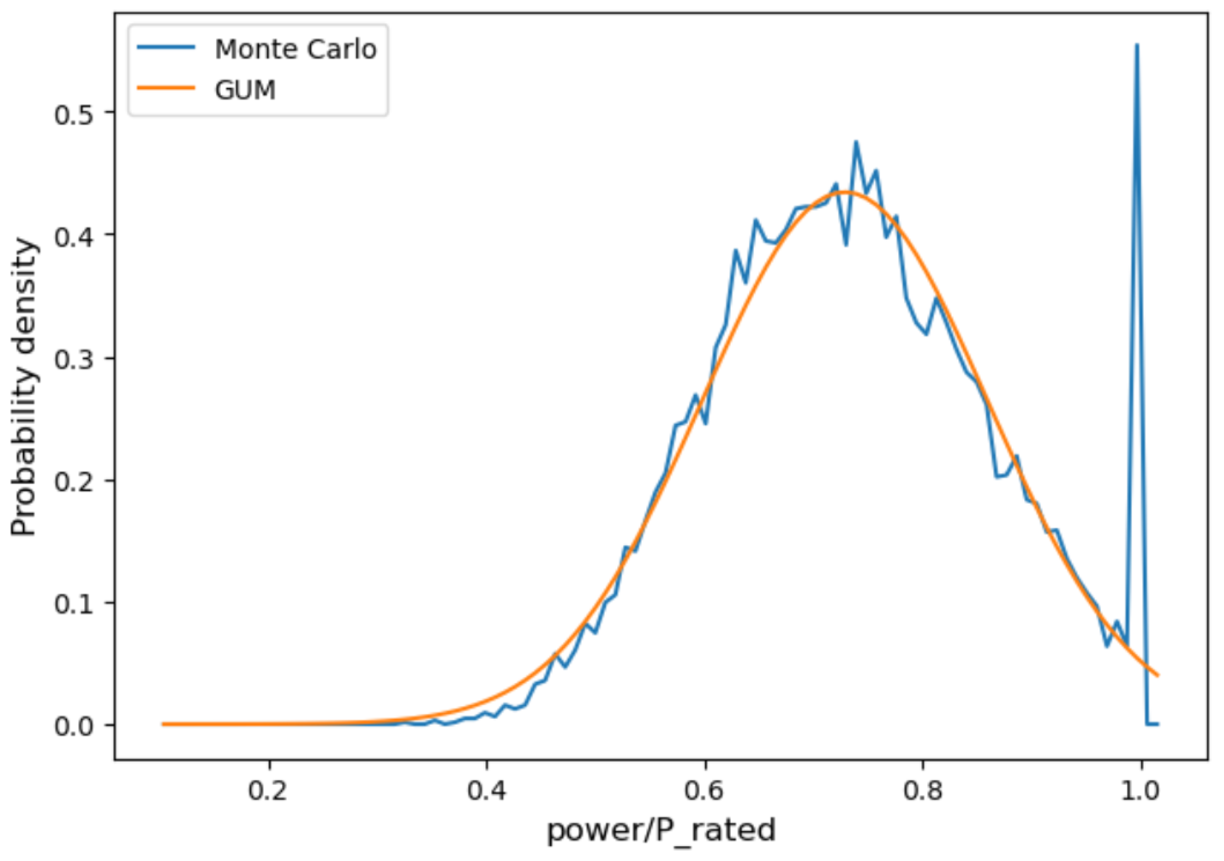
Figure 2.
Context of uncertainty quantification, with regards to propagation of uncertainty in a set of inputs through a model with model parameters and model uncertainty .
Figure 2.
Context of uncertainty quantification, with regards to propagation of uncertainty in a set of inputs through a model with model parameters and model uncertainty .
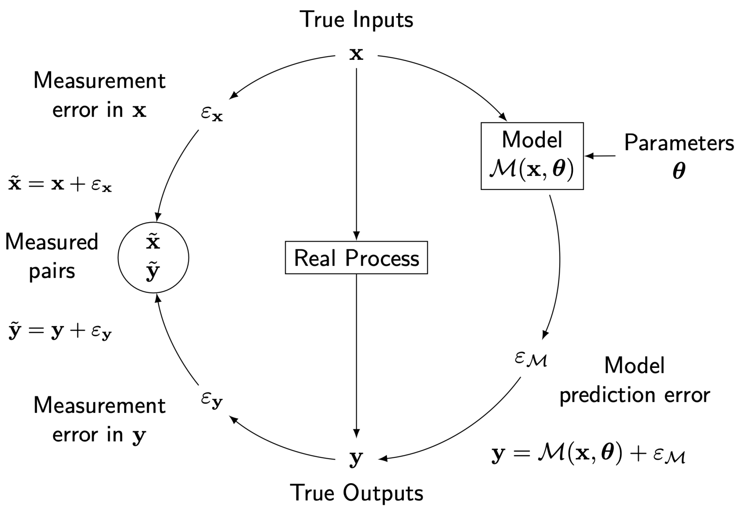
Figure 3.
Context of meteorology in wind energy, from a basic modelling perspective. Arrows indicate direction of information and propagation of uncertainty in a simple (decoupled, one-way) modelling methodology.
Figure 3.
Context of meteorology in wind energy, from a basic modelling perspective. Arrows indicate direction of information and propagation of uncertainty in a simple (decoupled, one-way) modelling methodology.
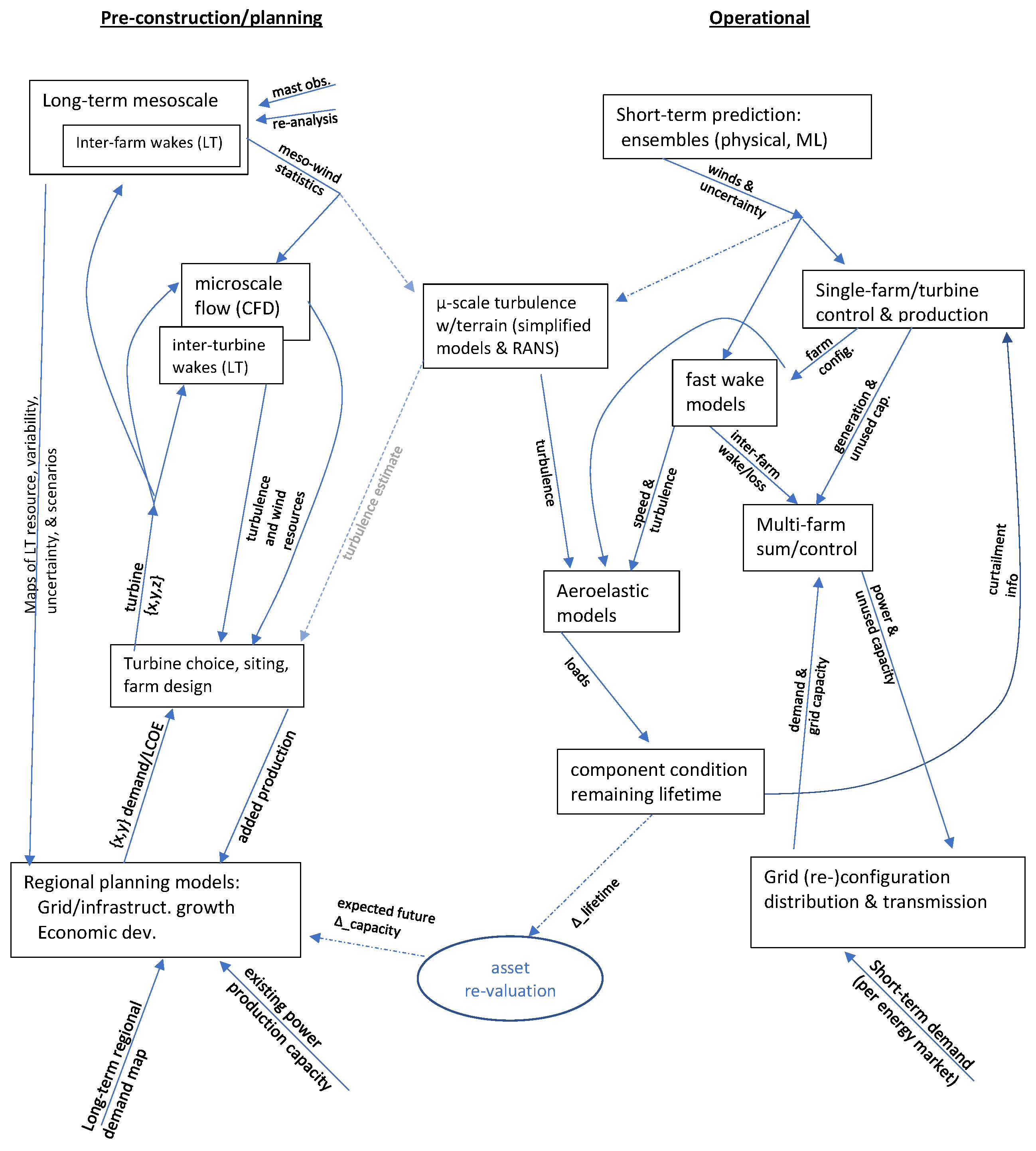
Figure 4.
Deviation in windfarm performance versus pre-construction uncertainty estimate, from wind farms with turbines of 1–3 MW from 2005–2014. Red and blue markers denote results from two different firms aggregated from [127]. Dotted lines are conditioned on pre-construction uncertainty, thick dashed line is mean, and straight green lines show ±1:1 relationship.
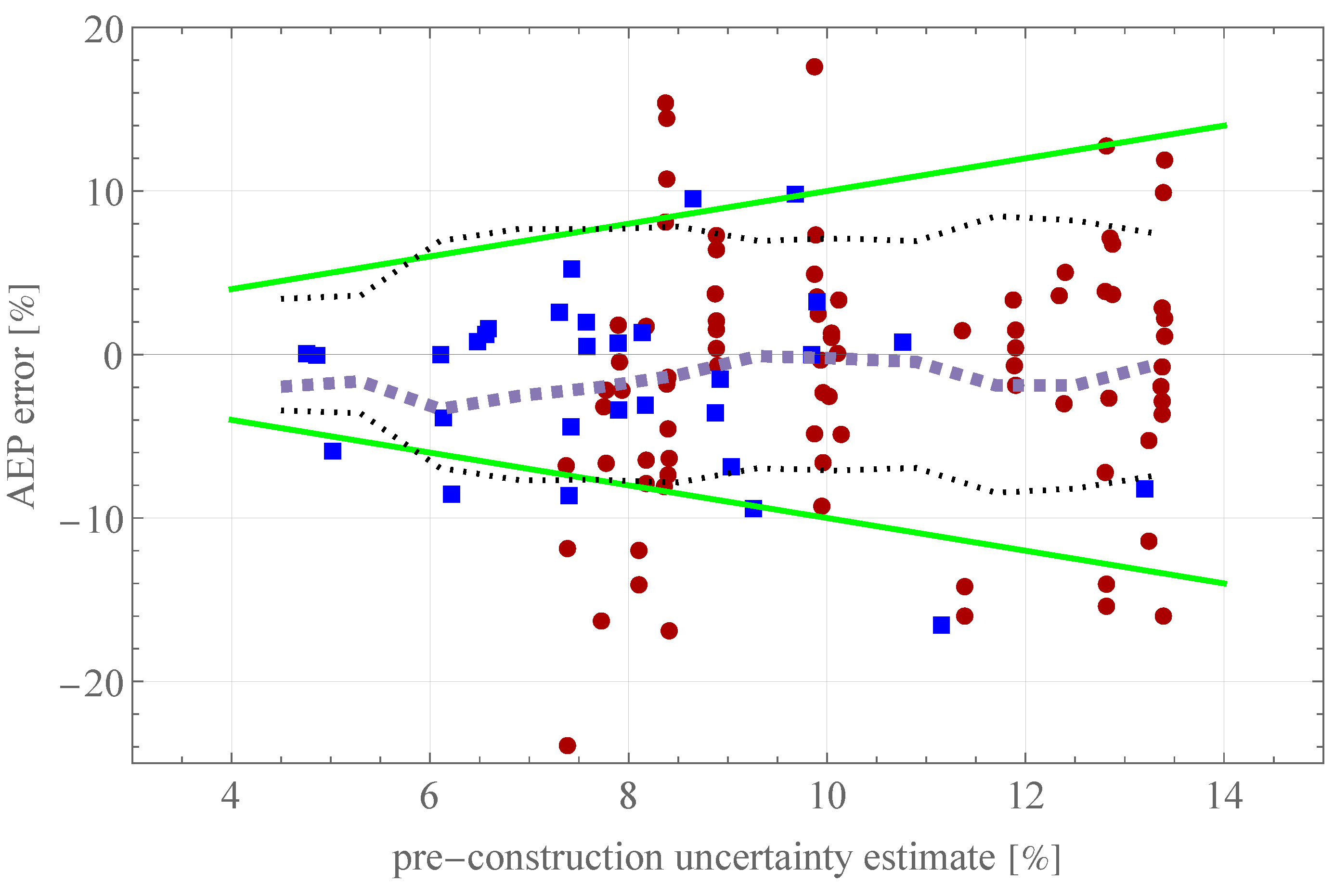

Table 1.
Uncertainty components and sub-components which depend on the wind; from the forthcoming IEC 61400-15-2 standard.
Table 1.
Uncertainty components and sub-components which depend on the wind; from the forthcoming IEC 61400-15-2 standard.
| Component (bold) or sub-component (italic) |
|---|
| Measurement Uncertainty |
| wind speed measurement |
| wind direction measurement / rose |
| other atmospheric parameters |
| data integrity and documentation |
| Historical Wind Resource (LTC) |
| representativeness of long-term reference period |
| reference data consistency |
| long-term correction method |
| on-site gap-filling/synthesis |
| representativeness of measured data |
| wind distribution fit |
| Horizontal Extrapolation and flow modelling |
| model inputs |
| model `stress’ (deviation from operational envelope) |
| model appropriateness |
| Vertical (power-law) Extrapolation |
| model representativeness† |
| excess uncertainty propagated by VE-model |
| Project Evaluation Period Variability |
| interannual variability (IAV) of wind speed |
| climate change |
| (IAV of plant performance)‡ |
| Plant Performance |
| Turbine interaction/wake and blockage effects |
| (non-wind elements)‡ |
† Through analytical derivation from the power-law, VE-model `stress’ is effectively an -dependence within the model representativeness subcomponent. ‡ Other non-wind plant performance uncertainty subcategories include turbine performance (power-curve), environmental (e.g., degredation), curtailment/operational strategy, availability, and electrical.
Disclaimer/Publisher’s Note: The statements, opinions and data contained in all publications are solely those of the individual author(s) and contributor(s) and not of MDPI and/or the editor(s). MDPI and/or the editor(s) disclaim responsibility for any injury to people or property resulting from any ideas, methods, instructions or products referred to in the content. |
© 2025 by the authors. Licensee MDPI, Basel, Switzerland. This article is an open access article distributed under the terms and conditions of the Creative Commons Attribution (CC BY) license (http://creativecommons.org/licenses/by/4.0/).
Copyright: This open access article is published under a Creative Commons CC BY 4.0 license, which permit the free download, distribution, and reuse, provided that the author and preprint are cited in any reuse.


